Electromagnetic field and radiation for a charge moving along a helical trajectory inside a waveguide with dielectric filling

Abstract

We investigate the electromagnetic field generated by a point charge moving along a helical trajectory inside a circular waveguide with conducting walls filled by homogeneous dielectric. The parts corresponding to the radiation field are separated and the formulae for the radiation intensity are derived for both TE and TM waves. It is shown that the main part of the radiated quanta is emitted in the form of the TE waves. Various limiting cases are considered. The results of the numerical calculations show that the insertion of the waveguide provides an additional mechanism for tuning the characteristics of the emitted radiation by choosing the parameters of the waveguide and filling medium.

PACS number(s): 41.60.Ap, 41.60.Bq

1 Introduction

A charged particle confined to the helical orbit is a source of high intensity electromagnetic radiation over a broad range of wavelengths with a number of remarkable properties such as high collimation and high degree of polarization (see, for instance Refs. [1, 2, 3]). These properties have resulted in extensive applications of this radiation in a wide variety of experiments and in many disciplines. In particular, the helical motion of an electron beam is employed in helical undulators to produce circularly polarized radiation in narrow angular cone in the forward direction [5, 6, 7, 8]. In the proposal of Ref. [4] the helical undulator radiation was used to generate a polarized positron beam. Synchrotron radiation from relativistic electrons spiralling in magnetic fields is the main mechanism to explain the emissions of many objects in radio astronomy (see [9] and references therein). Most of the works on the radiation from the helical trajectory refer to radiation in free space. It is well known that the presence of medium can essentially change the characteristics of the electromagnetic processes and gives rise to new types of phenomena such as the Cherenkov, transition, and diffraction radiations. In particular, the operation of a number of devices assigned to production of electromagnetic radiation is based on the interaction of charged particles with materials (see, for example, [10]).

The synchrotron radiation from a charged particle circulating in a homogeneous medium was considered in Ref. [11]. In this paper it was shown that the interference between the synchrotron and Cherenkov radiations leads to interesting effects. New interesting features arise in inhomogeneous media. In particular, the interfaces of media can be used to control the radiation flow emitted by various systems. In a series of papers started in Refs. [12, 13], we have considered the simplest geometries of boundaries between two dielectrics with spherical and cylindrical symmetries. The synchrotron radiation from a charge rotating around a dielectric ball enclosed by a homogeneous medium is investigated in Refs. [13, 14]. It was shown that if for the material of the ball and the particle velocity the Cherenkov condition is satisfied, strong narrow peaks appear in the radiation intensity. At these peaks the radiated energy exceeds the corresponding quantity in a homogeneous medium by several orders of magnitude. A similar problem with the cylindrical symmetry has been discussed in Refs. [12, 15, 16, 17]. In Ref. [12] we have developed a recurrent scheme for constructing the Green function of the electromagnetic field for a medium consisting of an arbitrary number of coaxial cylindrical layers. The investigation of the radiation from a charged particle circulating around a dielectric cylinder immersed in a homogeneous medium, has shown that under the Cherenkov condition for the material of the cylinder and the velocity of the particle, there are narrow peaks in the angular distribution of the number of quanta emitted into the exterior space. For some values of the parameters the density of the number of quanta in these peaks exceeds the corresponding quantity for the radiation in vacuum by several orders. The radiation by a longitudinal charged oscillator moving with a constant drift velocity along the axis of a dielectric cylinder immersed in a homogeneous medium is investigated in Refs. [18, 19]. As in the case of the circular motion it was shown that the presence of the cylinder provides a possibility for an essential enhancement of the radiation intensity. The properties of the radiation from a charged particle moving along a helical orbit in homogeneous dispersive medium are investigated in [20]. The corresponding problem for the charge moving in vacuum has been widely discussed in literature (see, e.g., Refs. [1, 2, 3, 21] and references given therein). The electromagnetic field and the radiation in the case of particle following the helical path inside a dielectric cylinder immersed into a homogeneous medium are studied in Refs. [22, 23]. Recently the influence of a homogeneous transparent medium on the radiation of relativistic particles in planar undulators is considered in Ref. [24].

In the present paper, we study the electromagnetic field and the radiation intensity for a charge moving in a helical orbit inside a circular waveguide with dielectric filling. Note that the radiation parts of the fields in the case of vacuum inside the waveguide are investigated in Ref. [25]. The plan of the paper is as follows. In section 2 we derive expressions for the electric and magnetic fields by making use of the corresponding formulae from [23] for the geometry of a dielectric cylinder immersed into a homogeneous medium. Analytic properties of the corresponding Fourier components are investigated. In section 3 the radiation fields are separated and they are presented as a superposition of the waveguide eigenmodes. The formulae are derived for the radiation intensity of TE and TM waves and numerical examples are presented. Section 4 concludes the main results of the paper.

2 Electromagnetic fields inside a waveguide

Consider a point charge $q$ moving along the helical trajectory of radius $\rho_{0}$ inside a circular waveguide with conducting walls. We will denote by $\rho_{1}$ the radius of the waveguide and will assume that it is filled by homogeneous dielectric with permittivity $\varepsilon_{0}$. The particle velocities along the axis of the waveguide (drift velocity) and in the perpendicular plane we denote by $v_{\parallel}$ and $v_{\perp}$, respectively. In a properly chosen cylindrical coordinate system ($\rho,\phi,z$) the corresponding motion is described by the coordinates

$$\rho=\rho_{0},\quad\phi=\omega_{0}t,\quad z=v_{\parallel}t,$$ (1)

where the $z$-axis coincides with the waveguide axis and $\omega_{0}=v_{\perp}/\rho_{0}$ is the angular velocity of the charge. This type of motion can be produced by a uniform constant magnetic field directed along the axis of a cylinder, by a circularly polarized plane wave, or by a spatially periodic transverse magnetic field of constant absolute value and a direction that rotates as a function of the coordinate $z$. In the helical undulators the last geometry is used.

In accordance with the symmetry of the problem, we present the electric and magnetic fields in the form of the Fourier expansion

$$F_{l}(\mathbf{r},t) = \sum_{m=-\infty}^{\infty}e^{im(\phi-\omega_{0}t)}\int_{-\infty}^{\infty}dk_{z}e^{ik_{z}(z-v_{\parallel}t)}F_{ml}(k_{z},\rho)$$ (2)

$$= 2{\mathrm{Re}}\sideset{}{{}^{\prime}}{\sum}_{m=0}^{\infty}e^{im(\phi-\omega_{0}t)}\int_{-\infty}^{\infty}dk_{z}e^{ik_{z}(z-v_{\parallel}t)}F_{ml}(k_{z},\rho),$$

where $l=\rho,\phi,z$, and in the discussion below $F=E,H$ for the electric and magnetic fields, respectively. The expressions for the Fourier transforms $F_{ml}(k_{z},\rho)$ are obtained from the corresponding formulae derived in Ref. [23] for the geometry of a dielectric cylinder with permittivity $\varepsilon_{0}$ immersed into a medium with permittivity $\varepsilon_{1}$, taking the limit $\varepsilon_{1}\rightarrow\infty$. As a result of this limiting procedure, the Fourier transforms are written in the decomposed form

$$F_{ml}(k_{z},\rho)=F_{ml}^{(0)}(k_{z},\rho)+F_{ml}^{(1)}(k_{z},\rho),$$ (3)

where the part $F_{ml}^{(0)}(k_{z},\rho)$ corresponds to the fields generated by the charge in a homogeneous medium with permittivity $\varepsilon_{0}$ and the part $F_{ml}^{(1)}(k_{z},\rho)$ is induced by the presence of the waveguide. In the case $\rho<\rho_{0}$ for the homogeneous part of the magnetic field one has

$$H_{ml}^{(0)} = -\frac{qk_{z}}{2\pi i^{\sigma_{l}}}\sum_{p=\pm 1}p^{\sigma_{l}-1}D_{m}^{(0p)}J_{m+p}(\lambda_{0}\rho),\;l=\rho,\phi,$$ (4)

$$H_{mz}^{(0)} = -\frac{q\lambda_{0}}{2\pi}\sum_{p=\pm 1}pD_{m}^{(0p)}J_{m}(\lambda_{0}\rho),$$ (5)

with the coefficients

$$D_{m}^{(0p)}=\frac{\pi}{2ic}\left[v_{\perp}H_{m+p}(\lambda_{0}\rho_{0})-v_{\parallel}\frac{\lambda_{0}}{k_{z}}H_{m}(\lambda_{0}\rho_{0})\right].$$ (6)

In these expressions $\sigma_{\rho}=1$, $\sigma_{\phi}=2$, $J_{m}(x)$ is the Bessel function, $H_{m}(x)=H_{m}^{(1)}(x)$ is the Hankel function of the first kind, and

$$\lambda_{0}^{2}=\frac{\omega_{m}^{2}(k_{z})}{c^{2}}\varepsilon_{0}-k_{z}^{2},\quad\omega_{m}(k_{z})=m\omega_{0}+k_{z}v_{\parallel}.$$ (7)

The corresponding expressions for $\rho<\rho_{0}$ are obtained from (4), (5) by the replacements $J\rightleftarrows H$. The part $H_{ml}^{(1)}(k_{z},\rho)$ induced by the presence of the waveguide is given by the formulae

$$H_{ml}^{(1)} = -\frac{qk_{z}}{2\pi i^{\sigma_{l}}}\sum_{p=\pm 1}p^{\sigma_{l}-1}D_{m}^{(p)}J_{m+p}(\lambda_{0}\rho),\;l=\rho,\phi,$$ (8)

$$H_{mz}^{(1)} = -\frac{q\lambda_{0}}{2\pi}\sum_{p=\pm 1}pD_{m}^{(p)}J_{m}(\lambda_{0}\rho),$$ (9)

where we have introduced the notation

$$D_{m}^{(p)} = \frac{\pi}{2ic}\left[v_{\parallel}\frac{\lambda_{0}}{k_{z}}\frac{H_{m}(\lambda_{0}\rho_{1})}{J_{m}(\lambda_{0}\rho_{1})}J_{m}(\lambda_{0}\rho_{0})-v_{\perp}J_{m+p}(\lambda_{0}\rho_{0})\frac{H_{m+p}(\lambda_{0}\rho_{1})}{J_{m+p}(\lambda_{0}\rho_{1})}\right.$$ (10)

$$\left.-\frac{iv_{\perp}p}{\pi\rho_{1}\lambda_{0}}\frac{J_{m-p}(\lambda_{0}\rho_{1})}{J_{m}(\lambda_{0}\rho_{1})J_{m}^{\prime}(\lambda_{0}\rho_{1})}\sum_{l=\pm 1}l\frac{J_{m+l}(\lambda_{0}\rho_{0})}{J_{m+l}(\lambda_{0}\rho_{1})}\right],$$

and the prime stands for the derivative with respect to the argument of the function.

The part in the electric field due to the presence of the waveguide is given by the formulae

$$E_{ml}^{(1)} = \frac{qci^{1-\sigma_{l}}}{4\pi\omega_{m}(k_{z})\varepsilon_{0}}\sum_{p=\pm 1}p^{\sigma_{l}}J_{m+p}(\lambda_{0}\rho)\left[\left(\frac{\omega_{m}^{2}(k_{z})\varepsilon_{0}}{c^{2}}+k_{z}^{2}\right)D_{m}^{(p)}-\lambda_{0}^{2}D_{m}^{(-p)}\right],$$ (11)

$$E_{mz}^{(1)} = \frac{qic\lambda_{0}k_{z}}{2\pi\omega_{m}(k_{z})\varepsilon_{0}}\sum_{p=\pm 1}D_{m}^{(p)}J_{m}(\lambda_{0}\rho),$$ (12)

where $l=\rho,\phi$. The corresponding formulae for the part $E_{ml}^{(0)}$ are obtained from (11), (12) by the replacement $D_{m}^{(p)}\rightarrow D_{m}^{(0p)}$. Note that in the limit $\rho_{0}\rightarrow\rho_{1}$ one has $D_{m}^{(p)}\rightarrow-D_{m}^{(0p)}$ and the fields vanish. We could expect this result, as when the charge is on the surface of the waveguide the charge and its image compensate each other.

The formulae given above describe the total electromagnetic field inside the waveguide. To separate the parts corresponding to the radiation we need the analytic properties of the Fourier components as functions on $k_{z}$. From formula (10) it follows that the function $D_{m}^{(p)}$ has singular points corresponding to the zeros of the function $J_{m}(\lambda_{0}\rho_{1})$ and its derivative. Note that in the second and third summands on the right of formula (10) the singularities at the zeros of the functions $J_{m\pm 1}(\lambda_{0}\rho_{1})$ cancel out and the function $D_{m}^{(p)}$ is analytic at these points. We denote by $j_{m,n}^{(\sigma)}$, $n=1,2,\ldots$, the $n$th positive zero of the Bessel function ($\sigma=0$) and its derivative ($\sigma=1$):

$$J_{m}^{(\sigma)}(\lambda_{0}\rho_{1})=J_{m}^{(\sigma)}(j_{m,n}^{(\sigma)})=0,$$ (13)

where $J_{m}^{(\sigma)}(x)=d^{\sigma}J_{m}(x)/dx^{\sigma}$. These zeros describe the eigenmodes for the cylindrical waveguide and are known as TM modes for the case $\sigma=0$ and as TE modes for the case $\sigma=1$ [26]. The corresponding modes for the projection of the wave vector on the cylinder axis are determined from the relation $\lambda_{0}\rho_{1}=j_{m,n}^{(\sigma)}$ by taking into account expressions (7):

$$\left(\beta_{\parallel}^{2}-1\right)k_{z}^{2}+2m\frac{\omega_{0}}{c}\sqrt{\varepsilon_{0}}\beta_{\parallel}k_{z}+\left(m^{2}\frac{\omega_{0}^{2}\varepsilon_{0}}{c^{2}}-\frac{j_{m,n}^{(\sigma)2}}{\rho_{1}^{2}}\right)=0,\;\beta_{\parallel}=\frac{v_{\parallel}}{c}\sqrt{\varepsilon_{0}}.$$ (14)

This equation has real solutions under the condition

$$b_{m,n}^{(\sigma)2}\left(1-\beta_{\parallel}^{2}\right)\leqslant 1,\;b_{m,n}^{(\sigma)}\equiv\frac{cj_{m,n}^{(\sigma)}}{m\omega_{0}\rho_{1}\sqrt{\varepsilon_{0}}},$$ (15)

and these solutions have the form

$$k_{z}=k_{m,n}^{(\sigma,\pm)}=\frac{m\omega_{0}\sqrt{\varepsilon_{0}}}{c\left(1-\beta_{\parallel}^{2}\right)}\left[\beta_{\parallel}\pm\sqrt{1+b_{m,n}^{(\sigma)2}\left(\beta_{\parallel}^{2}-1\right)}\right].$$ (16)

The values $k_{m,n}^{(\sigma,\pm)}$ correspond to the simple poles of the functions $E_{ml}(k_{z},\rho)$ and $H_{ml}(k_{z},\rho)$. Note that if the Cherenkov condition for the velocity of the particle along the axis of the waveguide is satisfied, $\beta_{\parallel}>1$, then inequality (15) is valid for all values $n=1,2,\ldots$. In the case $\beta_{\parallel}<1$, condition (15) determines the maximal value for $n$, which we will denote by $n_{\max}^{(\sigma)}$:

$$j_{m,n_{\max}^{(\sigma)}}^{(\sigma)}<\frac{m\omega_{0}\rho_{1}\sqrt{\varepsilon_{0}}}{c\sqrt{1-\beta_{\parallel}^{2}}}<j_{m,n_{\max}^{(\sigma)}+1}^{(\sigma)}.$$ (17)

The value of the function $\omega_{m}(k_{z})$ at the points $k_{m,n}^{(\sigma,\pm)}$ is equal to

$$\omega_{m,n}^{(\sigma,\pm)}=\frac{m\omega_{0}}{1-\beta_{\parallel}^{2}}\left[1\pm\beta_{\parallel}\sqrt{1+b_{m,n}^{(\sigma)2}\left(\beta_{\parallel}^{2}-1\right)}\right].$$ (18)

For $m=0$, equation (14) has real solutions only when $\beta_{\parallel}>1$ and

$$k_{z}=k_{0,n}^{(\sigma,\pm)}=\mp\frac{j_{0,n}^{(\sigma)}}{\rho_{1}\sqrt{\beta_{\parallel}^{2}-1}},\;\omega_{0,n}^{(\sigma,\pm)}=v_{\parallel}k_{0,n}^{(\sigma,\pm)}.$$ (19)

For real values $\varepsilon_{0}$ and under the condition (15) the poles are situated on the real axis of the complex plane $k_{z}$. In formula (2) it is necessary to give the way by which these poles should be circled. For this we note that in physical situations the dielectric permittivity is a complex quantity, $\varepsilon_{0}=\varepsilon_{0}^{\prime}+i\varepsilon_{0}^{\prime\prime}$, and the imaginary part $\varepsilon_{0}^{\prime\prime}$ determines the absorbtion in the medium. Under the condition $|\varepsilon_{0}^{\prime\prime}|\ll\varepsilon_{0}^{\prime}$, for the imaginary part of $k_{m,n}^{(\sigma,\pm)}$ from (16) one has

$${\mathrm{Im\,}}k_{m,n}^{(\sigma,\pm)}=\pm C_{1}\varepsilon_{0}^{\prime\prime}(\omega_{m}),\;C_{1}>0,$$ (20)

where $\varepsilon_{0}^{\prime\prime}(\omega_{m})\gtrless 0$ for $\omega_{m}\gtrless 0$. It can be also seen that $(b_{m,n}^{(\sigma)}-1){\mathrm{Re\,}}k_{m,n}^{(\sigma,-)}>0$. If the Cherenkov condition is not satisfied, $\beta_{\parallel}=v_{\parallel}\sqrt{\varepsilon_{0}^{\prime}}/c<1$, from the formulae given above it follows that

$${\mathrm{Re\,}}k_{m,n}^{(\sigma,+)}>0,\;\omega_{m}({\mathrm{Re\,}}k_{m,n}^{(\sigma,\pm)})>0,\;\pm{\mathrm{Im\,}}k_{m,n}^{(\sigma,\pm)}>0.$$ (21)

In this case the poles $k_{m,n}^{(\sigma,+)}$ ($k_{m,n}^{(\sigma,-)}$) are situated in the upper (lower) half of the complex plane $k_{z}$. In the limit $\varepsilon_{0}^{\prime\prime}\rightarrow 0$, deforming the integration contour we obtain the rule for avoiding the poles plotted in figure 1. In the case $\beta_{\parallel}>1$ the corresponding inequalities have the form

$${\mathrm{Re\,}}k_{m,n}^{(\sigma,+)}<0,\;\mp\omega_{m}({\mathrm{Re\,}}k_{m,n}^{(\sigma,\pm)})<0,\;{\mathrm{Im\,}}k_{m,n}^{(\sigma,\pm)}<0.$$ (22)

In the way similar to that for the previous case, deforming the contour for the integration over $k_{z}$, we obtain the avoidance rule for the poles given in figure 2.

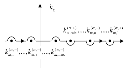
Figure 1: Integration contour in the $k_{z}$ plane for the case $\beta_{\parallel}<1$.

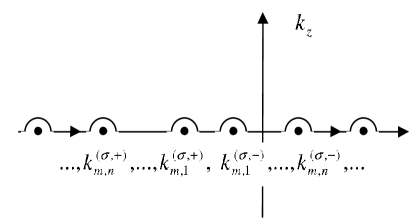
Figure 2: Integration contour in the $k_{z}$ plane for the case $\beta_{\parallel}>1$.

3 Radiation intensity in the waveguide

3.1 Radiation fields

In this section we consider the radiation field propagating inside a cylindrical waveguide with perfectly conducting walls for large distances from the charge. First of all let us show that the part corresponding to the first term on the right of formula (3) does not contribute to the radiation field. This directly follows from the estimate of the integral over $k_{z}$ on the base of the stationary phase method. As in the integral over $k_{z}$ the phase $k_{z}z$ has no stationary points, for large values $|z|$ the integral vanishes faster than any degree of $1/|z|$, under the condition that the preexponential function belongs to the class $C^{\infty}(R)$. It follows from here that the radiation field is determined by the singularity points of the preexponential function. As it has been mentioned before, for the integral over $k_{z}$ the only singular points are the poles of the function $D_{m}^{(p)}$ at the points $k_{z}=k_{m,n}^{(\sigma,\pm)}$, determined by relations (16). To find the corresponding contribution, we note that the integration contour over $k_{z}$ has the form depicted in figure 1 for $\beta_{\parallel}<1$ and the form depicted in figure 2 for the case $\beta_{\parallel}>1$. At large distances from the charge the integration contour can be closed by large semicircle in the upper (lower) half-plane for $z>v_{\parallel}t$ ($z<v_{\parallel}t$). This choice is caused by the fact that the integrand exponentially vanishes in the upper (lower) half-plane. As a result when the radius of the large semicircle goes to infinity the corresponding integral vanishes. Hence, for large values $|z|$ the integral over $k_{z}$, by residue theorem, is equal to the sum of residues inside the contour multiplied by $2\pi i\mathrm{sgn\,}(z-v_{\parallel}t)$. For $\varepsilon_{0}^{\prime\prime}\rightarrow 0$ and large $n$, when $b_{m,n}^{(\sigma)2}>\left(1-\beta_{\parallel}^{2}\right)$ ^-1, the poles $k_{m,n}^{(\sigma,\pm)}$ have a finite imaginary part and the corresponding contribution exponentially vanishes in the limit $z\rightarrow\infty$. As a result these poles do not contribute to the radiation field.

As before we consider two cases. When $\beta_{\parallel}<1$ we close the integration contour in figure 1 by the semicircle of large radius in the upper half-plane for $z>v_{\parallel}t$ and in the lower half-plane for $z<v_{\parallel}t$. As a result for the radiation field one finds

$$F_{l}(\mathbf{r},t)=\alpha{\mathrm{Re}}\left[\sum_{\sigma=0,1}\sideset{}{{}^{\prime}}{\sum}_{m=0}^{\infty}\sum_{n=1}^{n_{\max}^{(\sigma)}}F_{ml}^{(\sigma,\alpha)}(\mathbf{r},t)\right],$$ (23)

where $\alpha=+$   ($\alpha=-$) corresponds to the case $z>v_{\parallel}t$ ($z<v_{\parallel}t$) and we use the notation

$$F_{ml}^{(\sigma,\alpha)}(\mathbf{r},t)=4\pi i\underset{k_{z}=k_{m,n}^{(\sigma,\alpha)}}{\mathrm{Res}}F_{ml}(k_{z},\rho)e^{i(m\varphi+k_{z}z-\omega_{m}t)}.$$ (24)

Each term in the sum on the right of formula (23) describes waves with the frequency $\omega_{m,n}^{(\sigma,\pm)}$ propagating along the positive direction of the axis $z$ for $\alpha=+$ and for $\alpha=-$, $1<b_{m,n}^{(\sigma)}<1/\sqrt{1-\beta_{\parallel}^{2}}$, and waves propagating along the negative direction of the axis $z$ for $\alpha=-$, $b_{m,n}^{(\sigma)}<1$. If the Cerenkov condition is satisfied, $\beta_{\parallel}>1$, then closing the integration contour in figure 2 by large semicircle in the upper or lower half-plane in dependence of the sign for $z-v_{\parallel}t$, for the vector potential of the radiation field one finds

$$F_{l}(\mathbf{r},t)=-\theta(v_{\parallel}t-z){\mathrm{Re}}\left[\sum_{\alpha=\pm}\sum_{\sigma=0,1}\sideset{}{{}^{\prime}}{\sum}_{m=0}^{\infty}\sum_{n=1}^{n_{\max}^{(\sigma)}}F_{ml}^{(\sigma,\alpha)}(\mathbf{r},t)\right],$$ (25)

where $\theta(x)$ is the Heaviside unit step function. Separate terms in the sum in formula (25) describe waves with the frequency $|\omega_{m,n}^{(\sigma,\pm)}|$ propagating along the positive direction of the axis $z$ for $\alpha=+$ and for $\alpha=-$, $b_{m,n}^{(\sigma)}>1$, and along the negative direction of the axis $z$ for $\alpha=-$, $b_{m,n}^{(\sigma)}<1$. Note that for $b_{m,n}^{(\sigma)}>1$ we have no waves propagating along the negative direction of the axis $z$. By taking into account the formulae for the Fourier components of the fields and evaluating the residues by the standard formulae of the complex analysis, we find the following expressions for the radiation parts of the $z$-components of the fields:

$$E_{mz}^{(0,\alpha)}(\mathbf{r},t) = \frac{4qJ_{m}(j_{m,n}^{(0)}\rho_{0}/\rho_{1})}{\varepsilon_{0}\rho_{1}^{2}J_{m+1}^{2}(j_{m,n}^{(0)})}J_{m}(j_{m,n}^{(0)}\rho/\rho_{1})\exp[i(m\varphi+k_{m,n}^{(0,\alpha)}z-\omega_{m,n}^{(0,\alpha)}t)],$$ (26)

$$H_{mz}^{(1,\alpha)}(\mathbf{r},t) = -\alpha\frac{4iqv_{\perp}j_{m,n}^{(1)3}J_{m}^{\prime}(j_{m,n}^{(1)}\rho_{0}/\rho_{1})}{\sqrt{\varepsilon_{0}}\rho_{1}^{3}(j_{m,n}^{(1)}-m^{2})J_{m}^{2}(j_{m,n}^{(1)})}J_{m}(j_{m,n}^{(1)}\rho/\rho_{1})$$ (27)

$$\frac{\exp[i(m\varphi+k_{m,n}^{(1,\alpha)}z-\omega_{m,n}^{(1,\alpha)}t)]}{m\omega_{0}\sqrt{1+b_{m,n}^{(\sigma)2}\left(\beta_{\parallel}^{2}-1\right)}},$$

and $H_{mz}^{(0,\alpha)}(\mathbf{r},t)=E_{mz}^{(1,\alpha)}(\mathbf{r},t)=0$. The transverse components are found from the formulae

$$\mathbf{E}_{mt}^{(0,\alpha)}(\mathbf{r},t) = \frac{ik_{m,n}^{(0,\alpha)}}{j_{m,n}^{(0)2}}\rho_{1}^{2}\mathbf{\nabla}_{t}\psi^{(0)},\;\mathbf{H}_{mt}^{(0,\alpha)}(\mathbf{r},t)=\frac{\varepsilon_{0}\omega_{m,n}^{(0,\alpha)}}{ck_{m,n}^{(0,\alpha)}}\mathbf{e}_{3}\times\mathbf{E}_{mt}^{(0,\alpha)}(\mathbf{r},t),$$ (28)

$$\mathbf{H}_{mt}^{(1,\alpha)}(\mathbf{r},t) = \frac{ik_{m,n}^{(1,\alpha)}}{j_{m,n}^{(1)2}}\rho_{1}^{2}\mathbf{\nabla}_{t}\psi^{(1)},\;\mathbf{E}_{mt}^{(1,\alpha)}(\mathbf{r},t)=-\frac{\omega_{m,n}^{(1,\alpha)}}{ck_{m,n}^{(1,\alpha)}}\mathbf{e}_{3}\times\mathbf{H}_{mt}^{(1,\alpha)}(\mathbf{r},t),$$ (29)

where $\psi^{(0)}=E_{mz}^{(0,\alpha)}(\mathbf{r},t)$ and $\psi^{(1)}=H_{mz}^{(1,\alpha)}(\mathbf{r},t)$, $\mathbf{\nabla}_{t}=(\partial/\partial\rho,im/\rho,0)$, and $\mathbf{e}_{3}$ is the unit vector along the axis of the waveguide.

3.2 Radiation intensity

As we have seen, inside the waveguide the radiation is presented in the form of waves with discrete set of the values for the projection of the wave vector on the waveguide axis, $k_{z}=k_{m,n}^{(\sigma,\alpha)}$, $n=1,2,\ldots$, determined by formula (16). Having the radiation fields we consider the mean energy lost per unit time,

$$I=-\frac{1}{T}\int_{0}^{T}dt\int\left(j_{\varphi}E_{\varphi}+j_{z}E_{z}\right)\rho d\rho d\varphi dz,\;T=2\pi/\omega_{0}.$$ (30)

The radiation intensity $I$ is presented as the sum of intensities on separate modes:

$$I=\sideset{}{{}^{\prime}}{\sum}_{m=0}^{\infty}\sum_{\sigma=0,1}I_{m}^{(\sigma)},\;I_{m}^{(\sigma)}=\sum_{\alpha=\pm}\sum_{n=1}^{n_{\max}^{(\sigma)}}I_{m,n}^{(\sigma,\alpha)}.$$ (31)

The term with $m=0$ is present only then the condition $\beta_{\parallel}>1$ is satisfied and the corresponding parts have the form

$$I_{0}^{(0)}=\frac{2q^{2}v_{\parallel}}{\rho_{1}^{2}}\sum_{n=1}^{n_{\max}^{(0)}}\frac{J_{0}^{2}(j_{0,n}^{(0)}\rho_{0}/\rho_{1})}{\varepsilon_{0}J_{1}^{2}(j_{0,n}^{(0)})},\;I_{0}^{(1)}=\frac{2q^{2}v_{\perp}^{2}v_{\parallel}}{c^{2}\rho_{1}^{2}}\sum_{n=1}^{n_{\max}^{(1)}}\frac{J_{1}^{2}(j_{0,n}^{(1)}\rho_{0}/\rho_{1})}{\left(\beta_{\parallel}^{2}-1\right)J_{0}^{2}(j_{0,n}^{(1)})}.$$ (32)

Each term in the sums of these formulae corresponds to the radiation with the frequency given by the formula $v_{\parallel}j_{0,n}^{(\sigma)}/(\rho_{1}\sqrt{\beta_{\parallel}^{2}-1})$. For the radiation intensities on harmonics $m\neq 0$ one has the formulae

$$I_{m,n}^{(0,\alpha)} = \frac{2q^{2}c}{\varepsilon_{0}^{3/2}\rho_{1}^{2}}\frac{J_{m}^{2}(j_{m,n}^{(0)}\rho_{0}/\rho_{1})}{b_{m,n}^{(0)2}J_{m+1}^{2}(j_{m,n}^{(0)})}\frac{|\omega_{m,n}^{(0,\alpha)}|}{m\omega_{0}}\sqrt{1+b_{m,n}^{(0)2}\left(\beta_{\parallel}^{2}-1\right)},$$ (33)

$$I_{m,n}^{(1,\alpha)} = \frac{2q^{2}v_{\perp}^{2}}{c\sqrt{\varepsilon_{0}}\rho_{1}^{2}}\frac{j_{m,n}^{(1)2}J_{m}^{{}^{\prime}2}(j_{m,n}^{(1)}\rho_{0}/\rho_{1})}{\left(j_{m,n}^{(1)2}-m^{2}\right)J_{m}^{2}(j_{m,n}^{(1)})}\frac{|\omega_{m,n}^{(1,\alpha)}|}{m\omega_{0}\sqrt{1+b_{m,n}^{(1)2}\left(\beta_{\parallel}^{2}-1\right)}}.$$ (34)

For $\beta_{\parallel}<1$ the upper limit of the summation over $n$ is defined by relation (17). Otherwise this limit is determined by the dispersion law for the dielectric permittivity $\varepsilon_{0}$ through the condition $v_{\parallel}\sqrt{\varepsilon_{0}}>c$. It can be seen that for the case $\varepsilon_{0}=1$ the expression for $\sum_{\alpha}I_{m,n}^{(\sigma,\alpha)}$ obtained from formulae (33) and (34) coincides with the corresponding formulae in Ref. [25]. Taking $\beta_{\parallel}=0$, from formulae (33) and (34) we obtain the corresponding results for the radiation from a particle circulating in the plane perpendicular to the waveguide axis [28].

In accordance with (15), for given $m$ and $n$ the necessary condition for the presence of the radiation is the condition

$$m\omega_{0}\rho_{1}\sqrt{\varepsilon_{0}}/c\geqslant j_{m,n}^{(\sigma)}\sqrt{1-\beta_{\parallel}^{2}}.$$ (35)

Now by taking into account the relation $j_{m,n}^{(\sigma)}\geqslant m$ for the zeros of the Bessel functions, we conclude that under the conditions $\beta_{\parallel}<1$ and $\beta_{\perp}<\sqrt{1-\beta_{\parallel}^{2}}\rho_{0}/\rho_{1}$, with $\beta_{\perp}=v_{\perp}\sqrt{\varepsilon_{0}}/c$, there is no radiation inside the waveguide though the particle moves with acceleration. If $\beta_{\parallel}<1$ and the condition

$$j_{m,n}^{(\sigma)}\sqrt{1-\beta_{\parallel}^{2}}=m\beta_{\perp}\rho_{1}/\rho_{0}$$ (36)

takes place then the intensity for the TE waves defined by formulae (34) goes to infinity. However, under these conditions the absorption in the medium (and also in the walls of the waveguide) becomes important and the imaginary part of the dielectric permittivity should be taken into account. Formulae (33) and (34) are valid  under the condition

$$\frac{\varepsilon_{0}^{\prime\prime}}{\varepsilon_{0}^{\prime}}\ll\varepsilon_{0}^{\prime}\left[\left(\frac{m\omega_{0}\rho_{1}}{j_{m,n}^{(\sigma)}c}\right)^{2}+\frac{v_{\parallel}^{2}}{c^{2}}\right]-1,$$ (37)

where $\varepsilon_{0}=\varepsilon_{0}^{\prime}+i\varepsilon_{0}^{\prime\prime}$.

Instead of $k_{z}$ we can introduce the angular variable $\vartheta$, the values $\vartheta_{m,n}^{(\sigma,\alpha)}$ for which are related with the quantities $k_{m,n}^{(\sigma,\alpha)}$ by the formula

$$k_{m,n}^{(\sigma,\alpha)}=\frac{m\omega_{0}}{c}\frac{\sqrt{\varepsilon_{0}}\cos\vartheta_{m,n}^{(\sigma,\alpha)}}{1-\beta_{\parallel}\cos\vartheta_{m,n}^{(\sigma,\alpha)}}.$$ (38)

The quantities $\omega_{m}(k_{z})$ and $\lambda_{0}$ are expressed via $\vartheta_{m,n}^{(\sigma,\alpha)}$ by the formulae

$$\omega_{m}(k_{z}) = \frac{m\omega_{0}}{1-\beta_{\parallel}\cos\vartheta_{m,n}^{(\sigma,\alpha)}},$$ (39)

$$\lambda_{0} = \frac{\omega_{m}(k_{z})}{c}\sqrt{\varepsilon_{0}}\sin\vartheta_{m,n}^{(\sigma,\alpha)}.$$ (40)

The possible values $\vartheta_{m,n}^{(\sigma,\alpha)}$ are determined by formulae (16) and (38):

$$\cos\vartheta_{m,n}^{(\sigma,\pm)}=\frac{\beta_{\parallel}b_{m,n}^{(\sigma)2}\pm\sqrt{1+b_{m,n}^{(\sigma)2}\left(\beta_{\parallel}^{2}-1\right)}}{1+\beta_{\parallel}^{2}b_{m,n}^{(\sigma)2}}.$$ (41)

Note that the singularity in the radiation intensity (34) noted above corresponds to the values of the angular variable determined by the condition

$$\vartheta_{m,n}^{(\sigma,\alpha)}=\vartheta_{\perp},\;\vartheta_{\perp}\equiv\arccos\beta_{\parallel}.$$ (42)

In the reference frame moving along the direction of the axis $z$ with the velocity $v_{\parallel}$ the angle corresponding to $\vartheta_{\perp}$ is equal to $\pi/2$. From (41) the following relations can be seen

$$0\leqslant\vartheta_{m,n}^{(\sigma,+)}\leqslant\vartheta_{0}\leqslant\vartheta_{m,n}^{(\sigma,-)}\leqslant\pi,$$ (43)

where

$$\vartheta_{0}=\left\{\begin{array}[]{cc}\vartheta_{\perp}&\mathrm{for}\;\beta_{\parallel}<1,\\ \vartheta_{c}&\mathrm{for}\;\beta_{\parallel}>1,\end{array}\right.$$ (44)

and $\vartheta_{c}=\arccos(1/\beta_{\parallel})$ is the Cherenkov angle related to the drift velocity $v_{\parallel}$. Hence, for $\beta_{\parallel}<1$ the waves with $\alpha=+$ ($\alpha=-$) are those which in the reference frame moving with velocity $v_{\parallel}$ along the waveguide axis, propagate along the positive (negative) direction of the axis $z$. For $\beta_{\parallel}>1$ the waves with $\alpha=+$ ($\alpha=-$) propagate inside (outside) the Cherenkov cone $\vartheta=\vartheta_{c}$. From formulae (33), (34) it follows that the number of radiated quanta does not depend on $\alpha$. In particular, for $\beta_{\parallel}<1$, the same number of quanta is radiated inside and outside the cone $\vartheta=\vartheta_{\perp}$. For the case $\varepsilon_{0}=1$ we could expect this result from the problem symmetry, as in the reference frame moving along the direction of the axis $z$ with the velocity $v_{\parallel}$ we have a symmetric situation under the reflection with respect to the charge rotation plane.

Now let us consider the radiation intensity in the limiting case of large values of the waveguide radius, $\rho_{1}\rightarrow\infty$. In this limit the main contribution into the radiation intensity comes from large values $n$ and we can use the asymptotic formula (see, for instance, [27])

$$j_{m,n}^{(\sigma)}\approx\pi\left(n+\frac{m-1}{2}+\frac{(-1)^{\sigma}}{4}\right).$$ (45)

Replacing the summation over $n$ by the integration and introducing as a new integration variable the angle $\vartheta$, for the the radiation intensity one finds

$$I_{m}^{(\sigma)}\approx\int d\vartheta\frac{dI_{0m}^{(\sigma)}}{d\vartheta},$$ (46)

where

$$\frac{dI_{0m}^{(0)}}{d\vartheta} = \frac{q^{2}\omega_{0}^{2}m^{2}}{c\sqrt{\varepsilon_{0}}\sin\vartheta}\frac{(\cos\vartheta-\beta_{\parallel})^{2}}{|1-\beta_{\parallel}\cos\vartheta|^{3}}J_{m}^{2}\left(\frac{m\beta_{\perp}\sin\vartheta}{1-\beta_{\parallel}\cos\vartheta}\right),$$ (47)

$$\frac{dI_{0m}^{(1)}}{d\vartheta} = \frac{q^{2}\omega_{0}^{2}m^{2}}{c\sqrt{\varepsilon_{0}}}\frac{\beta_{\perp}^{2}\sin\vartheta}{|1-\beta_{\parallel}\cos\vartheta|^{3}}J_{m}^{\prime 2}\left(\frac{m\beta_{\perp}\sin\vartheta}{1-\beta_{\parallel}\cos\vartheta}\right).$$ (48)

In this limit the frequency for the radiation along given direction $\vartheta$ is determined by the expression $m\omega_{0}/|1-\beta_{\parallel}\cos\vartheta|$. The expressions (47) and (48) coincide with the corresponding formulae for the radiation in a homogeneous medium with dielectric permittivity $\varepsilon_{0}$. Note that in the discussed limit we have the transition $\vartheta_{m,n}^{(\sigma,\pm)}\rightarrow\vartheta$ and the upper (lower) sign corresponds to the angular region $0\leqslant\vartheta\leqslant\vartheta_{0}$ ($\vartheta_{0}\leqslant\vartheta\leqslant\pi$), where $\vartheta_{0}$ is defined by formula (44).

As an additional check for formulae (33), (34) we can consider the special case $\omega_{0}=0$ for a fixed value $\rho_{0}$. This corresponds to a charge moving with constant velocity $v_{\parallel}$ on a straight line $\rho=\rho_{0}$ parallel to the waveguide axis. In this limit $b_{m,n}^{(\sigma)}\rightarrow\infty$ and from condition (15) it follows that the radiation is present only under the Cherenkov condition $\beta_{\parallel}>1$. Taking the limit $\omega_{0}\rightarrow 0$, from formulae (33), (34) we see that

$$I_{m,n}^{(0,\alpha)}|_{\omega_{0}=0}=\frac{2q^{2}v_{\parallel}}{\varepsilon_{0}\rho_{1}^{2}}\frac{J_{m}^{2}(j_{m,n}^{(0)}\rho_{0}/\rho_{1})}{J_{m+1}^{2}(j_{m,n}^{(0)})},\;I_{m,n}^{(1,\alpha)}\rightarrow 0.$$ (49)

Hence, in the limit under consideration the TM waves are radiated only. The corresponding frequency is given by the expression $v_{\parallel}j_{m,n}^{(0)}/(\rho_{1}\sqrt{\beta_{\parallel}^{2}-1})$. In the limit $\rho_{1}\rightarrow\infty$, by using asymptotic formula (45) for the zeros of the Bessel function, replacing the summation over $n$ by the integration, and using the formula $\sideset{}{{}^{\prime}}{\sum}_{m=0}^{\infty}J_{m}^{2}(x)=1/2$, we can see that from (49) the formula for the Cherenkov radiation intensity in a homogeneous medium is obtained. Formula (49) for the radiation of a charge moving parallel to the axis of the waveguide can be found, for example, in [29].

We have carried out numerical calculations for the number of the radiated quanta per one period of the particle orbiting,

$$N_{m}^{(\sigma)}=\sum_{\alpha=\pm}\sum_{n=1}^{n_{\max}^{(\sigma)}}N_{m,n}^{(\sigma,\alpha)}=\frac{2\pi}{\hbar\omega_{0}}\sum_{\alpha=\pm}\sum_{n=1}^{n_{\max}^{(\sigma)}}\frac{I_{m,n}^{(\sigma,\alpha)}}{|\omega_{m,n}^{(\sigma,\alpha)}|}.$$ (50)

As it has been mentioned before, the quantity $N_{m,n}^{(\sigma,\alpha)}$ does not depend on $\alpha$. In figure 3 we have plotted the dependence of $N_{m}^{(\sigma)}$ on the ratio $\rho_{1}/\rho_{0}$ for $m=24$ and $v_{\perp}/c\approx 0.967$ corresponding to the energy 2 MeV assuming that $\varepsilon_{0}=3$. The graphs are given for $\beta_{\parallel}=0.9$ (left panel) and $\beta_{\parallel}=0.7$ (right panel). Note that the location of the peaks in the number of radiated quanta for TE waves is determined by formula (36). In particular, for large values $n$ by using the asymptotic formula (45) we see that the distance between the neighboring peaks is given by formula $\pi\sqrt{1-\beta_{\parallel}^{2}}/(m\beta_{\perp})$ and decreases with increasing $\beta_{\parallel}$. As we see the main part of the radiated quanta is emitted in the form of the TE waves. Similar features take place for the radiation on other values of the harmonic $m$. For the same values of the parameters, for the number $N_{0m}^{(\sigma)}$ of the radiated quanta in the homogeneous medium evaluated from formulae (47), (48), one finds

$$N_{0m}^{(0)} \approx 2.683\frac{q^{2}}{\hbar c},\;N_{0m}^{(1)}\approx 9.514\frac{q^{2}}{\hbar c},\;\mathrm{for}\;\beta_{\parallel}=0.9,$$ (51)

$$N_{0m}^{(0)} \approx 2.082\frac{q^{2}}{\hbar c},\;N_{0m}^{(1)}\approx 4.676\frac{q^{2}}{\hbar c},\;\mathrm{for}\;\beta_{\parallel}=0.7.$$ (52)

Of course, in this case the result does not depend on $\rho_{1}$.

Figure 3: The number of quanta emitted on the harmonic $m=24$ in the form of the TE and TM waves per circulating period of the charge, multiplied by $\hbar c/q^{2}$, $(\hbar c/q^{2})N_{m}^{(\sigma)}$, versus the ratio $\rho_{1}/\rho_{0}$ for $\beta_{\parallel}=0.9$ (left panel) and $\beta_{\parallel}=0.7$ (right panel). The velocity of the transverse motion corresponds to the energy 2 MeV and the dielectric permittivity is taken $\varepsilon_{0}=3$.

In addition to the total number of radiated quanta for a given $m$, it is of interest to consider the corresponding spectral distribution. On the left panel of figure 4 we have plotted the quantity $N_{m,n}^{(\sigma,\alpha)}$ as a function of $n$ for $\rho_{1}/\rho_{0}=1.02$, $\beta_{\parallel}=0.9$, for the same values of the parameters corresponding to figure 3. In this case we have $n_{\max}^{(\sigma)}=19$. On the right panel of figure 4 we have given the corresponding frequencies for TM and TE waves.

Figure 4: The left panel presents the number of radiated quanta, $(\hbar c/q^{2})N_{m,n}^{(\sigma,\alpha)}$, as a function of $n$ for the harmonic $m=24$ and for $\rho_{1}/\rho_{0}=1.02$, $\beta_{\parallel}=0.9$. The values of the other parameters are the same as those for figure 3. The black points correspond to the TE waves and the circles correspond to the TM waves. On the right panel the ratio $\omega_{m,n}^{(\sigma,\alpha)}/m\omega_{0}$ is plotted in dependence of $n$. The upper (lower) halves of the points correspond to $\alpha=+$ ($\alpha=-$). The values of the parameters are the same as for the left panel.

Now we consider an important case of relativistic charge motion in direction of the waveguide axis when the velocity of orthogonal motion is non-relativistic, $v_{\perp}\ll c$. This type of motion is realized in helical undulators. The corresponding magnetic field in Cartesian coordinates is given by $\mathbf{H}_{\mathrm{u}}=H_{\mathrm{u}}(-\sin(k_{\mathrm{u}}z),\cos(k_{\mathrm{u}}z),0)$, where $k_{\mathrm{u}}=2\pi/\lambda_{\mathrm{u}}$ and $\lambda_{\mathrm{u}}$ is the undulator period length. The corresponding parameters for the particle orbit are related to the particle energy $\mathcal{E}$ and to the undulator characteristics by the formulae

$$\frac{v_{\perp}}{c}=\frac{K_{\mathrm{u}}}{\gamma},\;\frac{v_{\parallel}}{c}=\sqrt{1-\frac{1+K_{\mathrm{u}}^{2}}{\gamma^{2}}},\;\omega_{0}=k_{\mathrm{u}}v_{\parallel},\;\rho_{0}=\frac{K_{\mathrm{u}}c}{\gamma k_{\mathrm{u}}v_{\parallel}},$$ (53)

where $\gamma=\mathcal{E}/m_{0}c^{2}$, with $m_{0}$ being the particle mass. In formulae (53), $K_{\mathrm{u}}=(q/m_{0}c^{2})H_{\mathrm{u}}/k_{\mathrm{u}}$ is the so-called undulator parameter. For example, for the helical undulator of the Stanford free electron laser $H_{\mathrm{u}}=0.23$ T, $\lambda_{\mathrm{u}}=3.3$ cm and the electron energy $\mathcal{E}=43.5$ MeV. For these values of the parameters we have $K_{\mathrm{u}}\approx 0.71$. As it is seen from (33), (34), in the presence of the medium the factor $1-v_{\parallel}^{2}/c^{2}$ in the formulae for the radiation intensity in the empty waveguide is replaced by the factor $1-\beta_{\parallel}^{2}$. This replacement leads to important influences on the radiation properties. These influences are essentially different in the cases $\varepsilon_{0}<1$ and $\varepsilon_{0}>1$. In the first case, even at very high energies the factor $1-\beta_{\parallel}^{2}$ tends to finite limiting value and the radiation does not have the features typical for the radiation of an ultrarelativistic particle in vacuum. In contrast to this, when $\varepsilon_{0}>1$, under the condition $0<1-\beta_{\parallel}^{2}\ll 1$ the properties of the radiation are similar to those for the radiation in vacuum from an ultrarelativistic particle even in the case when $v_{\parallel}$ is not too close to $c$. In order to illustrate these features, in figure 5 we have presented the number of the radiated quanta of the TE modes with $m=1$ as a function of the undulator parameter $K_{\mathrm{u}}$ for the undulator period $\lambda_{\mathrm{u}}=3$ cm and for the radius of the waveguide $\rho_{1}=0.5$ cm. The full curve corresponds to the radiation from an electron with the energy $\mathcal{E}=25$ MeV moving in the waveguide filled by air ($\varepsilon_{0}=1.00054$) and the dashed curve is for the radiation from an electron of energy 100 MeV moving in the empty waveguide ($\varepsilon_{0}=1$). Note that in the first case we have $1-\beta_{\parallel}\approx 4.1\times 10^{-5}$ and in the second case $1-\beta_{\parallel}\approx 1.9\times 10^{-5}$.

Figure 5: The number of the radiated quanta of the TE modes with $m=1$, $(\hbar c/q^{2})N_{1}^{(1)}$, as a function of the undulator parameter $K_{\mathrm{u}}$ for the undulator period $\lambda_{\mathrm{u}}=3$ cm and for the radius of the waveguide $\rho_{1}=0.5$ cm. The full curve corresponds to the radiation from an electron with the energy $\mathcal{E}=25$ MeV moving in the waveguide filled by air and the dashed curve is for the radiation from an electron of energy 100 MeV moving in the empty waveguide.

The corresponding spectral distributions are presented in figure 6 for the value of the undulator parameter $K_{\mathrm{u}}=0.7$. On the left panel we have plotted the quantity $N_{1,n}^{(1,\alpha)}$ as a function of $n$ and on the right panel the corresponding frequencies are presented. The black points correspond to the radiation from an electron with the energy $\mathcal{E}=25$ MeV moving in the waveguide filled by air and the circles correspond to the radiation from an electron of energy 100 MeV in the empty waveguide.

Figure 6: The left panel presents the number of the radiated quanta, $(\hbar c/q^{2})N_{1,n}^{(1,\alpha)}$, as a function of $n$ for $K_{\mathrm{u}}=0.7$. The values of the other parameters are the same as those for figure 5. On the right panel the corresponding frequencies, $10^{-13}\omega_{1,n}^{(1,\alpha)}/2\pi$, are plotted versus $n$. The black points correspond to the radiation from an electron with the energy $\mathcal{E}=25$ MeV moving in the waveguide filled by air and the circles correspond to the radiation from an electron of energy 100 MeV in the empty waveguide.

For ultrarelativistic particles the main part of the radiated energy is in the spectral range $\omega>\omega_{p}$ with $\omega_{p}$ being the plasma frequency, where the dielectric permittivity is well approximated by the formula $\varepsilon_{0}\approx 1-\omega_{p}^{2}/\omega^{2}$. In this regime the radiation frequencies are of the order $\omega_{0}\gamma^{2}$ and for the undulator parameter $\lambda_{u}\sim 1$ cm we have $\gamma\gtrsim 10^{3}$. In this range the perfect conductor boundary condition on the waveguide walls are no longer valid and for frequencies larger than the corresponding plasma frequency the waveguide becomes transparent. The corresponding radiation intensity propagating in the exterior region is strongly directed in the forward direction and is described by the formulae given in [22]. As regards the frequency range $\omega\ll\omega_{p}$ the corresponding radiation intensities are described by formulae (33), (34), where for materials with $\varepsilon_{0}-1\gg\gamma^{-2}$ we can substitute $1-\beta_{\parallel}^{2}\approx 1-\varepsilon_{0}$. By taking into account formula (53) for the radius of the helical orbit, from formulae (33), (34) we can see that for $j_{m,n}^{(\sigma)}\ll\gamma$ the number of the radiated quanta $N_{m,n}^{(\sigma,\alpha)}$ is suppressed by the factor $\gamma^{-2}$ for both TM and TE waves, whereas the corresponding frequencies are practically independent on the particle energy. For the modes with $j_{m,n}^{(\sigma)}\gtrsim\gamma$ we have $|\omega_{m,n}^{(\sigma,\alpha)}|\approx cj_{m,n}^{(\sigma)}/\sqrt{1-1/\varepsilon_{0}}\rho_{1}$ and $N_{m,n}^{(\sigma,\alpha)}\sim\gamma^{-2\sigma}$. In this case the radiation on the TM modes dominates.

In the discussion above we have considered the radiation emitted by a single particle moving along a prescribed trajectory. From the point of view of practical applications the generalization of the obtained results for the case of the radiation from an electron beam is a next important step. In helical undulators the beam is bunched and the features of the radiation critically depend on the ratio of the bunch length to the wavelength of the emitted radiation. If the wavelength is smaller than the bunch length the particles in the bunch are not phase correlated and the total power radiated by the bunch is the sum of single particle parts. In the opposite limit, called the coherent spontaneous radiation regime, the wavelength of the radiation exceeds the length of the bunch and the particles radiate coherently. In this case the radiated power is enhanced by the factor of number of particles in the bunch relative to the incoherent radiation at the same wavelength. Here it is important to take into account that long wavelength radiation is suppressed by the waveguide cutoff condition and this leads to the constraints for the bunch length in order to have coherent radiation in the waveguide. Once the fields are evaluated, another interesting question is related to the influence of the radiation field on the motion of the radiating particles. The interaction of the beam with its own radiation can induce an additional microbunching with the possibility of coherent radiation from particles of the same microbunch. These questions require a separate consideration and we plan to address them in the future work. A recent discussion of the beam dynamics in undulators can be found in [30] (see also [31]).

Another point which deserves a separate investigation is the role of the other processes of the particle interaction with the medium (see also the discussion in [24]). In particular, they include ionization energy losses, particle bremsstrahlung in media, and the multiple scattering (see, for instance, [32, 33]). The relative role of these processes depends on the particle energy and characteristics of the medium. To our best knowledge, the previous investigations in this direction were mainly concerned with the case of an unbounded homogeneous medium and the investigation of the effects induced by the presence of the waveguide requires a separate consideration. However, some general features can be obtained by using the corresponding results for a homogeneous medium. First of all, as the above-mentioned processes are absent in the vacuum, the radiation discussed in the present paper is the main mechanism of the energy losses in sufficiently rarefied medium. Next, while the ionization losses by an electron rise logarithmically with energy and bremsstrahlung losses arise nearly linearly, the undulator radiation intensity arises quadratically and, hence, dominates at sufficiently high energies. For a particle moving in air the ionization losses dominate those due to the bremsstrahlung for the energies less than 100 MeV. By using the standard formula, it can be seen that in the example corresponding to figures 5 and 6 the relative energy loss is $\approx 1\%$ per meter. An interesting possibility to escape ionization losses in the medium was indicated in [29] (see also [34]). In this paper it was argued that a narrow empty channel along the particle trajectory in the solid dielectric does not affect the radiation intensity if the channel radius is less than the radiation wavelength. From the other side, the maximum impact parameter for ionization losses is of the order $b_{\max}\sim\min[(\hbar/m_{0}c)\mathcal{E}/I,c/\omega_{p}]$, where $I$ is the mean excitation energy for the atom of the medium, and for the channel radius larger than $b_{\max}$ ionization losses are suppressed. As in other processes involving multiple scattering, we expect that this effect will appear in the formula for the radiation intensity at given frequency in the form of the additional multiplicative factor and there exists a critical energy of the particle below which the multiple scattering does not effect the radiation. We can try to estimate this factor by using the Migdal formula. For the values of the parameters taken in the example above this factor leads to the decrease of the radiation intensity by $\approx 0.5\%$.

4 Conclusion

We have investigated the electromagnetic field generated by a charge moving along a helical orbit inside a circular waveguide with dielectric filling. This type of motion is involved in magnetic devices called helical undulators which are inserted into a straight sector of storage rings. The helical undulators are used to generate circularly polarized intense electromagnetic radiation in a relatively narrow bandwidth. The frequency of radiation is tunable by varying the beam energy and the magnetic field. In this paper we have seen that the insertion of a waveguide into the helical undulator provides an additional mechanism for tuning the characteristics of the emitted radiation by choosing the parameters of the waveguide and filling medium. The electric and magnetic fields are presented as the sum of two parts. The first one corresponds to the fields of the charge in the homogeneous medium and the second one is induced by the presence of the waveguide. The Fourier components of the latter are given by formulae (8), (9), (11), (12). In order to extract from the total fields the parts corresponding to the radiation, we have investigated analytic properties of the Fourier components as functions on $k_{z}$. These components have poles on the eigenmodes of the waveguide. We have specified the ways by which these poles should be circled in the integral over $k_{z}$. For the cases $\beta_{\parallel}<1$ and $\beta_{\parallel}>1$ the corresponding contours are plotted in figures 1 and 2. By using the residue theorem, the radiation fields are presented as a superposition of the eigenmodes of the waveguide corresponding to the TM and TE waves. The projection of the wave vector on the waveguide axis and the corresponding frequency are given by formulae (16), (18). We have derived formulae (33) and (34) for the radiation intensity emitted in the form of the TM and TE waves. Limiting cases are considered and features of the radiation are investigated. In particular, we have seen that the main part of the radiated quanta is emitted in the form of the TE waves. Applications of general formulae to helical undulators are given. In particular, we have demonstrated that in the case of filled waveguide the radiation with features characteristic for ultrarelativistic particles in the empty waveguide is obtained for moderately relativistic particles. The radiation emitted on the waveguide modes propagates inside the cylinder and the waveguide serves as a natural collector for the radiation. This eliminates the necessity for focusing to achieve a high-power spectral intensity. The geometry considered here is of interest also from the point of view of generation and transmitting of waves in waveguides, a subject which is of considerable practical importance in microwave engineering and optical fiber communications.

References

- [1] A.A. Sokolov and I.M. Ternov, Radiation from Relativistic Electrons (ATP, New York, 1986).
- [2] Synchrotron Radiation Theory and Its Development, edited by V.A. Bordovitsyn (World Scientific, Singapore, 1999).
- [3] A. Hofman, The Physics of Sinchrotron Radiation (Cambridge University Press, Cambridge, 2004).
- [4] V.E. Balakin and A.A. Mikhailichenko, Preprint INP 79-85 (1979).
- [5] D.F. Alferov, Yu.A. Bashmakov, and E.G. Bessonov, Sov. Phys. Tech. Phys. 18, 1335 (1974).
- [6] B.M. Kincaid, J. Appl. Phys. 48, 2684 (1977).
- [7] P. Luchini and H. Motz, Undulators and Free-electron Lasers (Clarendon, 1990).
- [8] M.M. Nikitin and V.Ya. Epp, Undulator Radiation (Energoatomizdat, Moscow, 1988, in Russian).
- [9] G.B. Rybicky and A.P. Lightman, Radiative Processes in Astrophysics (J. Wiley, New York, 1979).
- [10] P. Rullhusen, X. Artru, and P. Dhez, Novel Radtiation Sources Using Relativistic Electrons (World Scientific, Singapore, 1998).
- [11] V.N. Tsytovich, Westnik MGU 11, 27 (1951, in Russian).
- [12] L.Sh. Grigoryan, A.S. Kotanjyan, and A.A. Saharian, Izv. Akad. Nauk Arm. SSR Fiz. 30, 239 (1995) [Sov. J. Contemp. Phys. 30, 1 (1995)].
- [13] S.R. Arzumanian, L.Sh. Grigoryan, Kh.V. Kotanjyan, and A.A. Saharian, Izv. Akad. Nauk Arm. SSR Fiz. 30, 106 (1995) [Sov. J. Contemp. Phys. 30, 12 (1995)].
- [14] L.Sh. Grigoryan, H.F. Khachatryan, and S.R. Arzumanyan, Izv. Akad. Nauk Arm. SSR Fiz. 33, 267 (1998) [Sov. J. Contemp. Phys. 33, 1 (1998)], cond-mat/0001322.
- [15] A.S. Kotanjyan, H.F. Khachatryan , A.V. Petrosyan, and A.A. Saharian, Izv. Akad. Nauk Arm. SSR Fiz. 35, (2000) [Sov. J. Contemp. Phys. 35, 1 (2000)].
- [16] A.S. Kotanjyan and A.A. Saharian, Izv. Akad. Nauk Arm. SSR Fiz. 36, 310 (2001) [Sov. J. Contemp. Phys. 36, 7 (2001)].
- [17] A.S. Kotanjyan, Nucl. Instrum. Methods B201, 3 (2003).
- [18] A.A. Saharian and A.S. Kotanjyan, Izv. Akad. Nauk Arm. SSR Fiz. 38, 288 (2003).
- [19] A.A. Saharian and A.S. Kotanjyan, Nucl. Instrum. Methods B226, 351 (2004).
- [20] L.A. Gevorgian and P.M. Pogosian, Izv. Akad. Nauk Arm. SSR Fiz. 19, 239 (1994).
- [21] A.A. Sokolov and I.M. Ternov, Zs. Phys. 211, 1 (1968).
- [22] A.A. Saharian and A.S. Kotanjyan, J. Phys. A 38, 4275 (2005).
- [23] A.A. Saharian, A.S. Kotanjyan, and M.L. Grigoryan, J. Phys. A 40, 1405 (2007).
- [24] S. Bellucci and V.A. Maisheev, J. Phys.: Condens. Matter 18, S2083 (2006).
- [25] G.G. Karapetyan, Izv. Akad. Nauk Arm. SSR Fiz. 12, 186 (1977).
- [26] J.D. Jackson, Classical Electrodynamics (John Wiley & Sons, 1998).
- [27] Handbook of Mathematical Functions, edited by M. Abramowitz and I.A. Stegun (Dover, New York, 1972).
- [28] A.S. Kotanjyan and A.A. Saharian, Mod. Phys. Lett. A 17, 1323 (2002).
- [29] B.M. Bolotovskii, Sov. Phys. Usp. 4, 781 (1961).
- [30] Undulators, Wigglers and Their Applications, edited by H. Onuki and P. Elleaume (Taylor & Francis, London, 2003).
- [31] K.Y. Ng, Physics of Intensity Dependent Beam Instabilities (World Scientific, Singapore, 2006).
- [32] M.L. Ter-Mikaelian, High Energy Electromagnetic Processes in Condensed Media (Wiley, New York, 1972).
- [33] A.I. Akhiezer and N.F. Shul’ga, High Energy Electrodynamics in Matter (Gordon and Breach, Amsterdam, 1996).
- [34] V.L. Ginzburg, Applications of Electrodynamics in Theoretical Physics and Astrophysics (Gordon and Breach, New York, 1989).