Invariants via word for curves and fronts

Abstract.

We construct the infinite sequence of invariants for curves in surfaces by using word theory that V. Turaev introduced. For plane closed curves, we add some extra terms, e.g. the rotation number. From these modified invariants, we get the Arnold’s basic invariants and some other invariants. We also express how these invariants classify plane closed curves. In addition, we consider other classes of plane curves: long curves and fronts.

1. Introduction

The object of the paper will be to construct some invariants of plane curves and fronts, and so it is to show one of the method for applying word theory to plane curves and fronts. V. Turaev introduces word theory ([Tu3], [Tu4], [Tu5]). We can consider that this word theory is effective in two view points as follows.

1. Word is the universal object of knot, curve, etc.

2. We can treat knots and curves collectively and algebraically, so that we can systematically study in these invariants themselves and relationships among them.

In terms of (1), Turaev applies topological methods (Reidemeister move, homotopy, etc.) to a semigroup consisting of letters, so that creates word which has property as (1) [Tu3]. In terms of (2), Turaev considers equivalent classes of words corresponding to knots or curves, and constructs invariants of knots, for example, Jones polynomial and $\underline{\alpha}$-kei which is similar to kei for knots [Tu4].

For immersed plane closed curves, H. Whitney classified plane closed curves regular homotopically by winding number, which is also called index or rotation number [W]. Long afterword, V. I. Arnold created three basic invariants of plane closed curves $J^{+},J^{-},St$ by the similar method to knots of V. A. Vassiliev [Va] and classified plane closed curves which have same index ([Ar1], [Ar2]). Arnold also obtained a natural generalization of $J^{+}$ to fronts ([Ar1], [Ar3]). Relating to this, M. Polyak systematically reconstructed the Arnold’s basic invariants via Gauss diagram and related basic invariants to the Vassiliev invariant [P].

In this paper, by using word theory, we will reconstruct the Arnold’s basic invariants and construct some other invariants for plane closed curves, long curves, and fronts. We also express how these invariants classify these plane curves and fronts.

The outline of each section is as follows. In Section 2, we will compose invariants $\{I_{n}\}$ (‘i’nvariant of degree ‘n’) of curves on a surface. In Section 3, we will construct invariants of plane closed curves $CI_{n}$ (‘c’losed curve ‘i’nvariant of degree‘n’) for $I_{n}$. $CI_{2}$ has the same strength as the Arnold’s basic invariants. $CI_{3}$ is independent of $CI_{2}$. There is an example that two curves take the same values of index, the Arnold’s basic invariants and HOMFLY polynomial of immersed plane closed curves [CGM] but take different values of $CI_{3}$. In Section 4, Section 5, we study in long curves and fronts by using the similar technique.

Conventions 1.

In this paper, all surfaces and curves are oriented. For a given surface $\varphi$, a closed curve (resp. long curve) is an immersion : $S^{1}$ (resp. $\mathbf{R}$) $\to$ $\varphi$ (resp. $\mathbf{R}^{2}$) where all of the singular points are transversal double points. A front is an immersion : $S^{1}$ $\to$ $\mathbf{R}^{2}$ with the coorientation (defined in Sect. 5.1) where all of the singular points are transversal double points or cusps. (We will precisely define a front in Sect. 5.1 . ) A curve is a closed curve, a long curve, or a front. A smooth curve is a closed curve or a long curve. When a curve stands for a closed curve or a front, a base point is a point on the curve except on the double points and the cusps. A pointed curve is a closed curve or a front endowed with a base point. Winding number (rotation number) is called index in this paper.

Acknowledgment 1.

I am grateful to Professor Jun Murakami for giving me numerous fruitful comments. This paper is nothing but trying to answer in my way to his question hitting the mark : “Can we apply word theory to plane curve theory?”

2. Invariants $\{I_{n}\}$

In this section we equip Turaev’s word to construct the sequence of invariants for pointed surface curves.

2.1. Turaev’s word

We follow the notation and terminology of [Tu4]. An alphabet is a set and its elements are called letters. A word of length $m\geq 1$ in an alphabet $\mathcal{A}$ is a mapping $\hat{m}=\{1,2,\ldots,m-1,m\}\to\mathcal{A}$. A word $w:\hat{m}\to\mathcal{A}$ is encoded by the sequence of letters $w(1)w(2)\cdots w(m)$. Two words $w$, $w^{\prime}$ are isomorphic if there is a bijection $w^{\prime}=fw.$

A word $w$ is called a Gauss word if each element of $\mathcal{A}$ is the image of precisely two elements of $\hat{m}$. For an alphabet $\alpha$, an $\alpha$-alphabet $\mathcal{A}$ is an alphabet endowed with a projection $|~{}|:\mathcal{A}\to\alpha$. An étale word over $\alpha$ is a pair $(\mathcal{A},w)$ where $\mathcal{A}$ is $\alpha$-alphabet and $w:\hat{m}\to\mathcal{A}.$ In this paper, we only treated étale word $(\mathcal{A},w)$ where $w$ is a surjection. In particular, a nanoword over $\alpha$ is an étale word $(\mathcal{A},w)$ over $\alpha$ where $w$ is a Gauss word. For $(\mathcal{A},w)$, we admit that we use the simple description ‘$w$’ if this $w$ means $(\mathcal{A},w)$ clearly. An isomorphism of $\alpha$-alphabets $\mathcal{A}_{1}$, $\mathcal{A}_{2}$ is a bijection $f:\mathcal{A}_{1}\to\mathcal{A}_{2}$ endowed with $|f(A)|=|A|$ for all $A\in\mathcal{A}_{1}$. Two nanowords $(\mathcal{A}_{1},w_{1})$, $(\mathcal{A}_{2},w_{2})$ over $\alpha$ are isomorphic if there is an isomorphism $f$ of $\alpha$-alphabets $\mathcal{A}_{1}$, $\mathcal{A}_{2}$ such that $w_{2}=fw_{1}.$

Until Sect. 4, we denote by ${\mathit{sign}}$ the projection $|~{}|$. We also define an alphabet $\alpha$, an involution $\tau$, and a set $S$ by

$$\alpha=\{-1,1\},\quad\tau:-1\mapsto 1,\quad S=\{(-1,-1,-1),(1,1,1)\}.$$

until Sect. 4.

The following fundamental theorem is established by Turaev [Tu4].

Theorem 2.1.

(Turaev) Every pointed closed curve is represented as a nanoword.

Proof.

For a given pointed closed curve which has precisely $m$ double points, we name the double points $A_{1},A_{2},\ldots,A_{m}$ along the curve orientation from the base point. Each point precisely corresponds to either $-1$ or $1$ in Figure 1. ∎

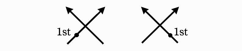
$-1$      $1$

Figure 1. Two patterns of the double points correspond to two letters in $\alpha$.

Remark 2.1.

Theorem2.1 implies that there is a mapping from a smooth curve $\Gamma$ on a surface to a nanoword. Conversely, there is a mapping from a nanoword to a smooth curve on a surface. In other words, we determine a unique smooth curve $\Gamma$ and a unique surface $\Sigma$ on which $\Gamma$ is by using the following Theorem2.2.

Theorem 2.2.

(Turaev) Let $w$ be a nanoword of length $n$ and $g(\Gamma)$ the minimum genus of the compact surface $\Sigma$ without boundary such that a pointed smmoth curve $\Gamma$ is on $\Sigma$. There is a mapping $w\mapsto\Gamma$ and

$$g(\Gamma)=1+\frac{n-card(\bar{n}/t\theta)}{2}.$$

The construction of the mapping $w\mapsto\Gamma$ is well known and therefore this is omitted (cf. [Tu1], [Tu2], [Vi]). We can calculate $g(\Gamma)$ by the proof of Theorem 9.1.1 in [Tu2] for Turaev’s chart.

2.2. Construction of invariants $I_{n}$

For every Gauss word $v$ and every nanoword $w$, we determine a number $\left\langle v,w\right\rangle$. When a nanoword $(\mathcal{A}_{w},w)$ over $\alpha$ is given, we consider a sub-word $v^{\prime}$ of $w$. If a sub-word $v^{\prime}$ is Gauss word, we can naturally consider the nanoword $(\mathcal{A}_{v^{\prime}},{v^{\prime}})$ over $\alpha$ such that $\mathcal{A}_{v^{\prime}}\subset\mathcal{A}_{w}$. Therefore for every nanoword $(\mathcal{A}_{w},w)$ over $\alpha$ and for every Gauss word $v$, we can define the mapping by

$$\left\langle v,w\right\rangle:=\sum_{\text{a sub-word $v^{\prime}$ of $w$ isomorphic to $v$}}\quad{\prod}_{A\in A_{v^{\prime}}}\mathit{sign}A.$$

Let $W_{n}$ be the free $\mathbf{Q}$-module generated by the set of all of the isomorphism class of the Gauss words where each length of the Gauss word is $2n$. For a given integer $d$, let $N_{d}$ be the free $\mathbf{Q}$-module generated by the set of nanowords over $\alpha$ where each length of the nanoword is less than $2d+1$. Expanding $\left\langle v,w\right\rangle$ bilinearly, we can make a bilinear mapping $\left\langle,\right\rangle$ from $W_{n}\times N_{d}$ to $\mathbf{Q}.$ For an arbitrary surface, let $w_{\Gamma}$ stand for a word which is determined by a curve $\Gamma$ on the surface.

Theorem 2.3.

The following $\{I_{n}\}$ (invariant of degree $n$) is the sequence of surface isotopy invariants for pointed curves on a surface.

$$I_{n}(\Gamma)=\left\langle\sum_{k}x_{k}v_{k},w_{\Gamma}\right\rangle\qquad(n\in\mathbf{N})$$

where $\{v_{k}\}$ is the basis of $W_{n}$ and each $x_{k}$ is a parameter.

Proof.

By using Theorem 2.1, the way of constructing $\langle,\rangle$ implies this theorem. ∎

2.3. Generalization of $I_{n}$

We can generalize $I_{n}$ by introducing a dimension of a letter.

Definition 2.1.

(a dimension of a letter, a dimension of a word) Let $X$, $\dot{X}$ be letters. For an arbitrary letter $A$, we denoted by $d(A)\in\{1,2\}$ a dimension of a letter $A$ which is defined by the following. Let $X$ be a $1$-dimensional letter where $d(X)=1$ and let $\dot{X}$ a 2-dimensionl letter where $d(\dot{X})=2$. Next, let $\mathcal{A}$ be an alphabet. For every word $w:\hat{m}\to\mathcal{A}$, the dimension $d(w)$ of word $w$ is defined by $d(w):=\sum_{X\in\mathcal{A}}d(X)$.

The concept of the dimension of word affect on the module ‘$W_{n}$’. That is why we must redefine ‘$W_{n}$’.

The following word space $\mathcal{W}_{n}$ is the canonical generalization of ‘$W_{n}$’ defined in Sect. 2.2.

Definition 2.2.

(word space) The word space $\mathcal{W}_{n}$ of degree $n$ is the free $\mathbf{Q}$-module generated by the set of all of the $n$-dimensional Gauss words which may contain $2$-dimensional letters.

Replacing $W_{n}$ defined in Sect. 2.2 with $\mathcal{W}_{n}$, we can easily check that the similar results are established and can easily generalize Sect. 2.2.

For an arbitrary $(\mathcal{A}_{w},w)$ and $v\in\mathcal{W}_{n}$, we think of $(\mathcal{A}_{v^{\prime}},{v^{\prime}})$ where $v^{\prime}$ is a sub-word of $w$ which is isomorphic to $v$ and $\mathcal{A}_{v^{\prime}}\subset{A}_{w}$. We redefine $\left\langle,\right\rangle$ by

$$\left\langle v,w\right\rangle:=\sum_{\text{a sub-word $v^{\prime}$ of $w$ isomorphic to $v$}}\quad\prod_{A\in A_{v}}\left(\mathit{sign}A\right)^{d(A)}.$$

Corollary 2.1.

The following $\{GI_{n}\}$ (generalized $I_{n}$) is the sequence of surface isotopy invariants for pointed curves on a surface.

$$GI_{n}(\Gamma)=\left\langle\sum_{k}x_{k}v_{k},w_{\Gamma}\right\rangle\qquad(n\in\mathbf{N})$$

where $\{v_{k}\}$ is the basis of the word space $W_{n}$ and each $x_{k}$ is a parameter.

Remark 2.2.

For every plane closed curve $\Gamma$, $\left\langle\dot{X}\dot{X},w_{\Gamma}\right\rangle$ is the number of the double points for $\Gamma$ [P].

3. Application of $I_{n}$ to plane closed curves

We will consider an application of $I_{n}$ to plane closed curve. We can apply word theory to plane curve theory because word is universal for knots and curves. In this section we will apply it to plane closed curve for example. Plane curves are not only fundamental objects but also proper objects to think of some various applications of word theory. In fact, we can apply word theory to closed curves, long curves, and fronts (Sect. 4, 5). When we apply word theory to plane closed curves, we get some invariants $CI_{n}$ (‘c’losed curve ‘i’nvariant degree $n$). In order to construct $CI_{n}$, to add to Turaev’s word, we need one more material about plane curve theory : the Arnold’s basic invariants defined in the next subsection.

3.1. The Arnold’s basic invariants

We consider regular homotopy classes of plane curves. Let us rewrite the Arnold’s the invariants via Turaev’s word theory. To redefine the Arnold’s basic invariants [Ar2], we define elementary moves that are local moves (Figure 2, 3) of plane curves apart from a base point.

Definition 3.1.

(elementary move) Let $x,y,z$ be words that consist of the letter in $\mathcal{A}$ where $\mathcal{A}\cap\{A,B\}=\emptyset$. Elementary move $I\!I^{+}$ and elementary move $I\!I^{-}$ (Figure 2) are defined by

$$I\!I^{+}:(\mathcal{A},xyz)\to(\mathcal{A}\cup\{A,B\},xAByABz)~{}\text{if}~{}\tau({\mathit{s}ign}A)={\mathit{s}ign}B,$$

$$I\!I^{-}:(\mathcal{A},xyz)\to(\mathcal{A}\cup\{A,B\},xAByBAz)~{}\text{if}~{}\tau({\mathit{s}ign}A)={\mathit{s}ign}B.$$

Let $x,y,z,t$ be words that consist of the letter in $\mathcal{A}-\{A,B,C\}$. Elementary move $I\!I\!I$ (Figure 3) is defined by

$$(\mathcal{A},xAByACzBCt)\to(\mathcal{A},xBAyCAzCBt)~{}\text{for}~{}({\mathit{s}ign}A,{\mathit{s}ign}B,{\mathit{s}ign}C)\in S.$$

The positive elementary moves is the above direction, the negative elementary move is the inverse direction.

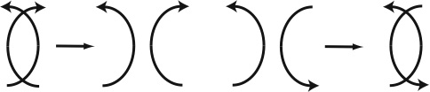
Figure 2. Positive elementary move $I\!I^{+}$ (left figure) and Positive elementary move $I\!I^{-}$ (right figure).

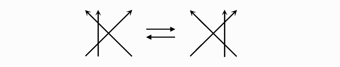
Figure 3. Elementary move $I\!I\!I$. If the order of three branch are 1, 2, 3 from the left, the direction of the positive move is from the left figure to the right figure. If the order of three branch are 3, 2, 1 from the left, the direction of the positive move is from the right figure to the left figure.

For this elementary moves, the Arnold’s basic invariants $J^{+},J^{-},St$ are invariants of curve can be defined by following (cf. [Ar2]).

Definition 3.2.

(the Arnold’s basic invariants) $J^{+}$ is increased by 2 under positive elementary move $I\!I^{+}$ but not change under the other, $J^{-}$ is decrease by 2 under positive elementary move $I\!I^{-}$ but not change under the other, $St$ is increased by 1 under positive elementary move $I\!I\!I$ but not change under the other, and satisfy the following conditions

$$J^{+}(K_{0})=0,\quad J^{-}(K_{0})=-1,\quad St(K_{0})=0,$$

$$J^{+}(K_{i+1})=-2i,\quad J^{-}(K_{i+1})=-3i,\quad St(K_{i+1})=i$$

for the base curves $\{K_{i}\}$ defined by Figure 4.

$K_{0}$        $K_{1}$      $K_{2}$       $K_{3}$       $K_{4}$

Figure 4. Base curve $\{K_{i}\}$.

3.2. Construction of invariants $\overline{CI}_{n}$

In this subsection, we compose a mapping $\left[,\right]$ to construct invariants $\overline{CI}_{n}$ of plane closed curves. To add to $\left\langle,\right\rangle$, we equip cyclic equivalent to construct a mapping $\left[,\right].$

Definition 3.3.

(cyclic equivalent) Let $x$ be $w(2)$ $\cdots$ $w(m)$ of $w$ $=$ $w(1)$$w(2)$ $\cdots$ $w(m)$, for two arbitrary Gauss words $w,w^{\prime}\in W_{n}$, the relation $\sim$ is defined by

$$w\sim w^{\prime}\stackrel{{\scriptstyle\mathrm{def}}}{{\Longleftrightarrow}}w=Ax~{}\text{and}~{}w^{\prime}=-xA.$$

This relation $\sim$ is called cyclic equivalent.

The cyclic equivalent is equivalent relation. Let $\overline{W}_{n}$ be a module consisting of cyclic equivalent classes of the elements of $W_{n}$ (defined by Sect. 2.2). For $[w]\in\overline{W}_{n}$, the number of the residue system of $[w]$ is even. That is because $w\sim-w$ implies $w\sim 0$ if this number is odd.

The mapping

$$\left[,\right]:\overline{W}_{n}\times N_{d}\to\mathbf{Q}$$

is defined by

$$\left[[v],w\right]:=\left<v_{1}+v_{2}+\cdots+v_{2l},w\right>$$

where $v_{1},v_{2},\ldots,v_{2l}$ consist of all elements of $[v]$.

Proposition 3.1.

Let $\Gamma$ be an arbitrary curve. For every $[w]\in\overline{W}_{n}$, $[[w],w_{\Gamma}]$ is a surface isotopy invariant of curves.

Proof.

Base point move (Figure 5) is , that is to say, to replace $(\mathcal{A},w_{\Gamma})=AxAy$ with $xA_{\tau}yA_{\tau},{\mathit{s}ign}{A_{\tau}}=\tau({\mathit{s}ign}A)$ where $x,y$ are consist of the letters of $\mathcal{A}-\{A\}$.

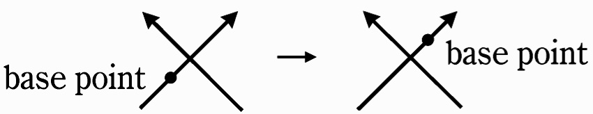
Figure 5. Base point move.

Therefore under the base point move, a part of $\left<AxAy,w_{\Gamma}\right>$ multiplied -1 is added to $\left<xAyA,w_{\Gamma}\right>$. By definition of cyclic equivalence, and by the new numbering

$v_{1},v_{2},\ldots,v_{2l}$ if necessary, we can have

$$v_{1}\stackrel{{\scriptstyle\text{base point move}}}{{\to}}v_{2}\stackrel{{\scriptstyle\text{base point move}}}{{\to}}\cdots\stackrel{{\scriptstyle\text{base point move}}}{{\to}}v_{2l}\stackrel{{\scriptstyle\text{base point move}}}{{\to}}v_{1}.$$

therefore, the value of $\left<v_{1}+v_{2}+\cdots+v_{2l},w_{\Gamma}\right>$ is not change by base point move. ∎

Corollary 3.1.

The following $\{\overline{I}_{n}\}$ is the sequence of surface isotopy invariants for closed curves on a surface.

$$\overline{I}_{n}(\Gamma):=\left[\sum_{k}x_{k}[v_{k}],w_{\Gamma}\right]\qquad(n\in\mathbf{N}).$$

$\{[v_{k}]\}$ is the base of $\overline{W}_{n}$, and each $x_{k}$ is a parameter.

In particular, for every closed plane curve, the following $\{\overline{CI}_{n}\}$ is the sequence of plane isotopy invariants.

$$\overline{CI}_{n}(\Gamma):=\overline{I}_{n}(\Gamma)+f(i)\qquad(n\in\mathbf{N})$$

where f is function of index i.

Next subsection, we introduce $CI_{2}$ and $CI_{3}$ which are made of $\overline{CI}_{2}$ and $\overline{CI}_{3}$.

3.3. $CI_{2}$ and $CI_{3}$

For every curve $\Gamma$, let $i$ be index and $n$ the number of the double points, we define $CI_{2}$ by

$$CI_{2}(\Gamma;s,t,u):=sn+\left\langle tXXYY-tXYYX+uXYXY,w_{\Gamma}\right\rangle+\frac{t}{2}-\frac{t}{2}i^{2}.$$

Remark 3.1.

$\overline{CI}_{2}(\Gamma)=\left[t[XXYY],w_{\Gamma}\right]$, and then, we have

$$CI_{2}(\Gamma;s,t,u)=\overline{CI}_{2}(\Gamma)+sn+\left\langle uXYXY,w_{\Gamma}\right\rangle+\frac{t}{2}-\frac{t}{2}i^{2}.$$

M. Polyak proved that $\left\langle XYXY,w_{\Gamma}\right\rangle$ does not depend on the choice of a base point (cf. Theorem 1 proof in [P]). Therefore the invariant $CI_{2}$ is well-defined. $CI_{2}$ is also not depend on the orientation of the curve $\Gamma$ because this formula is symmetric. $CI_{2}(\Gamma;s,t,u)$ is substituted by $CI_{2}(\Gamma)$ if this means $CI_{2}(\Gamma;s,t,u)$ clearly. Similarly, for other invariants in this paper we admit the abbreviation like this if its meaning is clear.

Theorem 3.1.

(Polyak) $CI_{2}$ is an invariant of plane curves which is as strong as the triple of the three Arnold’s basic invariants $(J^{+},J^{-},St)$. (The definitions of $J^{+},J^{-},St$ are in [Ar1], [Ar2], [P]. )

Proof.

By using Polyak’s formulation of the Arnold basic invariants [P], the triple of the three Arnold’s basic invariants $\left(J^{+}(\Gamma),J^{-}(\Gamma),St(\Gamma)\right)$ is equal to

$$\left(CI_{2}(\Gamma;-\frac{1}{2},1,-3),CI_{2}(\Gamma;-\frac{3}{2},1,-3),CI_{2}(\Gamma;\frac{1}{4},-\frac{1}{2},\frac{1}{2})\right)$$

and three vectors $(-\frac{1}{2},1,-3),(-\frac{3}{2},1,-3),(\frac{1}{4},-\frac{1}{2},\frac{1}{2})$ are linearly independent. These two facts imply this theorem. ∎

Remark 3.2.

Index is independent of the basic invariants (cf. Figure 6).

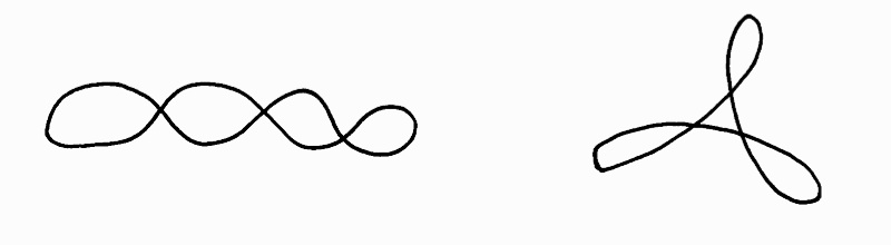
Figure 6. $CI_{2}$ is $3s+\frac{3}{2}t$ on both curves, but the value of index is $0$ for the left figure, $2$ for the right figure.

We represent

$$XYXYZZ-YXYZZX+XYZZXY-YZZXYX+ZZXYXY-ZXYXYZ,$$

as $[XYXYZZ]$ and represent $XXYYZZ-XYYZZX$ as $[XXYYZZ].$

For every curve $\Gamma$, let $i$ be index, and we define $CI_{3}$ by

$$CI_{3}(\Gamma;s,t):=\left[s[XYXYZZ]+t[XXYYZZ],w_{\Gamma}\right]+i.$$

Remark 3.3.

$CI_{3}(\Gamma;s,t)=\overline{CI}_{3}(\Gamma;s,t)+i.$

Theorem 3.2.

$CI_{3}$ is an invariant of plane closed curves.

Proof.

To prove this, we must prove that $CI_{3}(\Gamma)$ is not varied by an arbitrary base point move (Figure 5) for every closed curve $\Gamma$, but it is immediately concluded by Proposition 3.1. ∎

There exist two curves such that the values of the HOMFLY polynomial of immersed plane curves [CGM], index, basic invariants are the same; however, the value of $CI_{3}$ on one curve is different from that on the other (Figure 7).

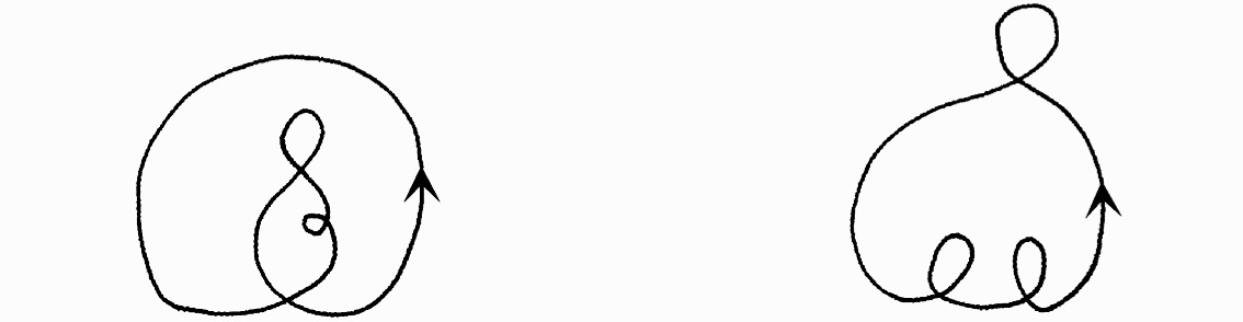
Figure 7. Two curves such that the value of the HOMFLY polynomial is $x^{2}z_{2}$ and $(i,J^{+},J^{-},St)$ is $(2,-4,-7,2)$. The value of $CI_{3}$ is $t+2$ for the left figure, $-t+2$ for the right figure.

This example implies the following.

Corollary 3.2.

$CI_{3}$ is independent of index, the Arnold’s basic invariants and the HOMFLY polynomial of immersed plane curves.

As can be seen from the examples above (the case of $CI_{2}$ and $CI_{3}$), we can get some invariants by the normalization of $\overline{CI}_{n}$. We denote by $CI_{n}$ a normalized invariants which is made of $\overline{CI}_{n}$.

Corollary 3.3.

Suppose $-\Gamma$ has only difference of orientation from $\Gamma$, and let $\Gamma^{r}$ be the reflection of $\Gamma$,

$$CI_{3}(-\Gamma)=-CI_{3}(\Gamma),\quad CI_{3}(\Gamma^{r})=-CI_{3}(\Gamma).$$

Remark 3.4.

$$CI_{2}(-\Gamma)=CI_{2}(\Gamma).$$

3.4. Strengthening $CI_{n}$

We can strengthen $CI_{n}$ by the similar method of $GI_{n}$ in Sect. 2.3. We must define marked cyclic equivalent which is the canonical generalization of cyclic equivalent defined in Sect. 3.2.

Definition 3.4.

(marked cyclic equivalent) Let $x$ be $w(2)$ $\cdots$ $w(m)$ of $w$ $=$ $w(1)$$w(2)$ $\cdots$ $w(m)$, for two arbitrary Gauss words $w,w^{\prime}\in W_{n}$, relation $\sim$ is defined by

$$w\sim w^{\prime}\stackrel{{\scriptstyle\mathrm{def}}}{{\Longleftrightarrow}}\left\{\begin{array}[]{ll}w=Ax~{}\text{and}~{}w^{\prime}=-xA&\text{if}~{}d(A)=1\\ w=\dot{A}x~{}\text{and}~{}w^{\prime}=x\dot{A}&\text{if}~{}d(A)=2\end{array}\right.$$

This relation $\sim$ is called marked cyclic equivalent.

Replacing cyclic equivalent by marked cyclic equivalent, we can easily check that the similar results are established and can easily generalize Sect. 3.2. Therefore we only see the case of $CI_{3}$.

For every curve $\Gamma$, let $i$ be index, and we define $GCI_{3}$ by

$GCI_{3}(\Gamma;s,t,u):=\left[s[XYXYZZ]+t[XXYYZZ]+u[\dot{X}\dot{X}YY],w_{\Gamma}\right]+i.$

Remark 3.5.

$GCI_{3}(\Gamma;s,t,u)=CI_{3}(\Gamma;s,t)+\left[u[\dot{X}\dot{X}YY],w_{\Gamma}\right].$

Corollary 3.4.

$GCI_{3}$ is an invariant of plane curves.

Example 3.1.

There exist two curves such that the value of $CI_{3}$, index, basic invariants are the same; however, the value of $GCI_{3}$ on one curve is different from that on the other (Figure 8).

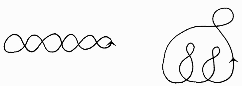
Figure 8. Two curves such that $($$CI_{3},$ $i,$ $J^{+},$ $J^{-},$ $St$$)$ is $($$0,$ $0,$ $0,$ $-5,$ $0$$)$. The value of $GCI_{3}$ is $0$ for the left figure, $-8u$ for the right figure.

In particular, this example implies the following.

Corollary 3.5.

$GCI_{3}$ is a stronger invariant than $CI_{3}.$

4. Application of $I_{n}$ to long curves

4.1. Construction of invariants $LI_{n}$

When we treated long curves via word theory, the following theorem is basic and fundamental.

Theorem 4.1.

Every long curve is represented as a nanoword.

Proof.

Regard $-\infty$ on x-axis as a base point and repeat the proof of Theorem 2.1. ∎

Let $i$ be index. By Theorem 4.1, we get the sequence of invariants of long curves $\{LI_{n}\}$ defined by $LI_{n}=I_{n}+i$.

Remark 4.1.

For an arbitrary function of index $i$, $I_{n}+f(i)$ is plane isotopy invariant.

4.2. The basic invariants of long curves

In similar way of defining the Arnold’s basic invariants of plane closed curve in Sect. 3.1, we define the basic invariants of long curves in this subsection (cf. [GN], [ZZP]).

Definition 4.1.

(basic invariants of long curves) $J^{+}$ is increased by 2 under positive elementary move $I\!I^{+}$ but not change under the other, $J^{-}$ is decrease by 2 under positive elementary move $I\!I^{-}$ but not change under the other, $St$ is increased by 1 under positive elementary move $I\!I\!I$ but not change under the other, and satisfy the following conditions

$$J^{+}(L_{i})=-\left|i\right|,\quad J^{-}(L_{i})=-2\left|i\right|,\quad St(L_{i})=\frac{1}{2}\left|i\right|$$

for the base curves $\{L_{i}\}$ defined by Figure 9.

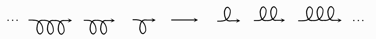
$L_{-3}$     $L_{-2}$    $L_{-1}$     $L_{0}$    $L_{1}$     $L_{2}$     $L_{3}$

Figure 9. Base curve $\{L_{i}\}.$

4.3. $LI_{2}$ and $LI_{3}$

For long curve L, let $i$ be index and $n$ the number of double points, we define $LI_{2}$ by

$$LI_{2}(L;s,t,u,v):=sn+\left\langle tXXYY+uXYYX+vXYXY,w_{L}\right\rangle-\frac{t}{2}i^{2}$$

As case of $CI_{2}$, $LI_{2}$ is not depend on the orientation of long curve L.

Theorem 4.2.

$LI_{2}$ is an invariant of plane curves which is as strong as $(J^{+},J^{-},St)$.

In other words, for two arbitrary long curves $L_{1}$, $L_{2}$,

$$LI_{2}(L_{1})=LI_{2}(L_{2})\Longleftrightarrow(J^{+}(L_{1}),J^{-}(L_{1}),St(L_{1}))=(J^{+}(L_{2}),J^{-}(L_{2}),St(L_{2})).$$

Before we begin proving Theorem4.2, we will prove Lemma 4.1. (Similar formula is concluded in case closed curves [P]. )

Lemma 4.1.

$$LI_{2}(L;\frac{1}{2},1,1,1)=\frac{n}{2}+\left\langle XXYY+XYYX+XYXY,w_{L}\right\rangle-\frac{i^{2}}{2}\equiv 0$$

In particular, left side is independent of elementary move I​I and I​I​I.

Proof.

For $w_{L}=(\mathcal{A},w_{L})$, we have $i=\sum_{A\in\mathcal{A}}{\mathit{sign}}A$. Therefore

$$i^{2}=\left(\sum_{A\in\mathcal{A}}\mathit{sign}A\right)^{2}=\left\langle\dot{X}\dot{X}+2XXYY+2XYYX+2XYXY,w_{L}\right\rangle.$$

The number of double points $n$ is equal to $\left\langle\dot{X}\dot{X},w_{L}\right\rangle$. ∎

Next, we will prove Theorem 4.2. It is sufficient that we prove the following.

Proof.

( $\Longrightarrow$). The following three relations are concluded by Proposition 4.1.

Proposition 4.1.

$$J^{+}(L) = LI_{2}(L;-\frac{1}{2},1,-1,-3),$$

$$J^{-}(L) = LI_{2}(L;-\frac{3}{2},1,-1,-3),$$

$$St(L) = LI_{2}(L;\frac{1}{4},-\frac{1}{2},\frac{1}{2},\frac{1}{2}).$$

(Proof of Proposition 4.1. ) Let $n$ be the number of double points and $f(i)$ a function on index $i$. By using Theorem 2.3,

$I_{2}(L;s,t,u,v)=ns+\left\langle tXXYY+uXYYX+vXYXY\right\rangle-t\frac{i^{2}}{2}$

is an invariant of long curves.

By definition of $J^{+},J^{-},St$,

$$J^{+}(L) = LI_{2}(L;s,2s+2,2s,2s-2),$$

$$J^{-}(L) = LI_{2}(L;s,2s+4,2s+2,2s),$$

$$St(L) = LI_{2}(L;s,2s-1,2s,2s).$$

These $J^{+}(L),J^{-}(L),St(L)$ satisfies

$$J^{+}(L_{i})=-\left|i\right|,\quad J^{-}(L_{i})=-2\left|i\right|,\quad St(L_{i})=\frac{1}{2}\left|i\right|.$$

Especially, In the case $s=-\frac{1}{2}$ on $J^{+}$, in the case $s=-\frac{3}{2}$ on $J^{-}$, in the case $s=-\frac{1}{4}$ on St, these are still the basic invariants. We have thus proved the Proposition 4.1 that implies ($\Longleftarrow$).

($\Longleftarrow$). For two arbitrary long curves $L_{1}$, $L_{2}$, assume

$$(J^{+}(L_{1}),J^{-}(L_{1}),St(L_{1}))=(J^{+}(L_{2}),J^{-}(L_{2}),St(L_{2})).$$

Four vectors $(\frac{1}{2},1,1,1)$, $(-\frac{1}{2},1,-1,-3)$, $(-\frac{3}{2},1,-1,-3)$, $(\frac{1}{4},-\frac{1}{2},\frac{1}{2},\frac{1}{2})$ are linearly independent. By adding Lemma 4.1 and Proposition 4.1, the assumption implies $LI_{2}(L_{1})$ $=$ $LI_{2}(L_{2})$. ∎

Remark 4.2.

Index is independent of the basic invariants. (cf. Figure 10).

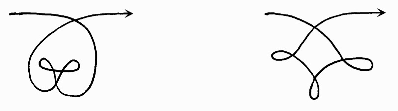
Figure 10. $LI_{2}$ is $4s+t-3u$ on both curves, but the value of index is $0$ for the left figure, $2$ for the right figure.

Remark 4.3.

If $n$ of them are not same, the values of $LI_{2}$ for two curves are not the same because $J^{+}-J^{-}=n$.

For every long curve $L$, let $i$ be index, we define $LI_{3}$ by

$$LI_{3}(L;x_{1},x_{2},\ldots,x_{14},x_{15}) := \langle x_{1}XYXYZZ+x_{2}XYXZZY+x_{3}XYZZXY$$

$$+x_{4}XYYZXZ+x_{5}XXYZYZ+x_{6}XYZYZX$$

$$+x_{7}XYYXZZ+x_{8}XXYZZY+x_{9}XYZZYX$$

$$+x_{10}XYZYXZ+x_{11}XYXZYZ+x_{12}XYZXZY$$

$$+x_{13}XYZXYZ+x_{14}XXYYZZ+x_{15}XYYZZX,$$

$$w_{L}\rangle+i.$$

Theorem 4.3.

$LI_{3}$ is an invariant of long curves.

Proof.

Theorem 2.3 immediately deduces this conclusion. ∎

Corollary 4.1.

Let $L^{r}$ be the reflection of a long curve $L$, $LI_{3}(L^{r})=-LI_{3}(L)$.

Remark 4.4.

$LI_{2}(L^{r})=LI_{2}(L)$.

The following are examples of several pairs of long curves such that the values of index and three basic invariants are the same, but the value of $LI_{3}$ on one long curve is different from that on the other.

Example 4.1.

For $L_{1}$, $L_{1}^{r}$, $L_{2}$, $L_{2}^{r}$ (Figure 11) such that $(i,J^{+},J^{-},St)$ is $(0,0,-4,0)$, each value of $LI_{3}$ is different from another of them.

$L_{1}$       $L_{1}^{r}$      $L_{2}$       $L_{2}^{r}$

Figure 11. Four long curves such that $(i,J^{+},J^{-},St)=(0,0,-4,0).$ $LI_{3}(L_{1})$ $=$ $2x_{7}$ $-$ $x_{14}$ $-$ $x_{15},$ $LI_{3}(L_{1}^{r})$ $=$ $-2x_{7}$ $+$ $x_{14}$ $+$ $x_{15},$ $LI_{3}(L_{2})$ $=$ $2x_{8}$ $-$ $x_{14}$ $-$ $x_{15},$ $LI_{3}(L_{2}^{r})$ $=$ $-2x_{8}$ $+$ $x_{14}$ $+$ $x_{15}.$

Example 4.2.

For $L_{3}$, $L_{4}$, $L_{5}$, $L_{6}$ (Figure 12) such that $($$i,$ $J^{+},$ $J^{-},$ $St$$)$ $=$ $($$2,$ $-4,$ $-8,$ $2)$, each value of $LI_{3}$ is different from another of them.

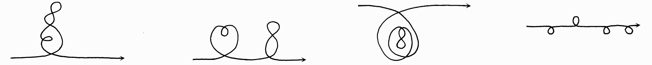
$L_{3}$       $L_{4}$      $L_{5}$       $L_{6}$

Figure 12. Four long curves such that $($$i,$ $J^{+},$ $J^{-}$ $St$$)$= $($$2,$ $-4,$ $-8,$ $2$$)$. $LI_{3}(L_{3})$ $=$ $-x_{7}$ $-$ $x_{9}$ $+$ $2,$ $LI_{3}(L_{4})$ $=$ $-2x_{8}$ $+$ $2,$ $LI_{3}(L_{5})$ $=$ $2x_{9}$ $+$ $2,$ $LI_{3}(L_{6})$ $=$ $2x_{14}$ $+$ $2.$

4.4. Strengthening $LI_{n}$

We can strengthen $LI_{n}$ in the way constructing $GI_{n}$ in Sect. 2.3.

For every long curve $L$, let $i$ be index, we define $GLI_{3}$ by

$$GLI_{3}(L;x_{1},x_{2},\ldots,x_{20},x_{21}) := LI_{3}(L;x_{1},x_{2},\ldots,x_{14},x_{15})$$

$$+\langle x_{16}\dot{X}\dot{X}YY+x_{17}\dot{X}YY\dot{X}+x_{18}XX\dot{Y}\dot{Y}$$

$$+x_{19}X\dot{Y}\dot{Y}X+x_{20}X\dot{Y}X\dot{Y}+x_{21}\dot{X}Y\dot{X}Y,w_{L}\rangle.$$

Corollary 4.2.

$GLI_{3}$ is an invariant of long curves.

Example 4.3.

There exist two curves such that the value of $LI_{3}$, index, basic invariants are the same; however, the value of $GLI_{3}$ on one curve is different from that on the other (Figure 13).

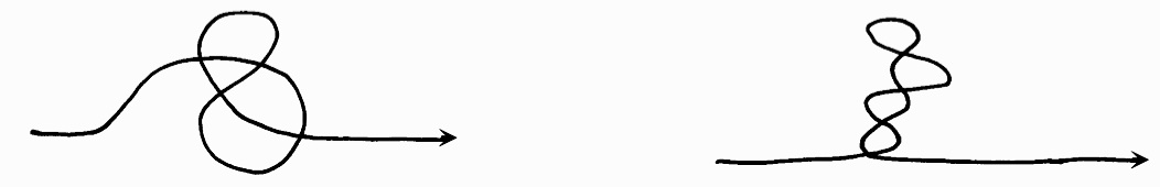
Figure 13. Two curves such that $($$LI_{3},$ $i,$ $J^{+},$ $J^{-},$ $St$$)$ is $($$0,$ $0,$ $0,$ $-4,$ $0$$)$. The value of $GLI_{3}$ is $0$ for the left figure, $-2x_{17}$ $+$ $2x_{19}$ for the right figure.

In particular, this example implies the following.

Corollary 4.3.

$GLI_{3}$ is a stronger invariant than $LI_{3}.$

4.5. The Arnold-type invariant of degree 3

Definition 4.2.

(The Arnold-type invariant of degree 3) Let $J^{+}$-type invariant be an invariant do not change under elementary move $I\!I^{-}$, $I\!I\!I$, $J^{-}$-type invariant be an invariant do not change under elementary move  $I\!I^{+}$, $I\!I\!I$, $St$-type invariant be an invariant do not change under elementary move  $I\!I^{+},I\!I^{-}$.

$J^{+}$-type invariant, $St$-type invariant are available from $GLI_{3}$. These are expressed $J^{+}_{3}$ ($J^{+}$ of degree 3), $St_{3}$ ($St$ of degree 3).

Theorem 4.4.

Let L be long curve.

$$J^{+}_{3}(L) = GLI_{3}(L;s+t-v,s-t+u,-s+t+v,-s+3t-u,s+t-v,$$

$$2t-v,s,s,t,u,2t-v,-2s+4t-u,-2s+2t+v,s-t+v,$$

$$\frac{1}{2}t,\frac{1}{2}s,v,\frac{1}{2}s,\frac{1}{2}t,-s+2t-\frac{1}{2}u,\frac{1}{2}u),$$

$$St_{3}(L) = GLI_{3}(L;2u,p,2s,q,2x,2y,2u,2x,2y,2z,r,2z,2z,s,t,u,v,x,y,z,z).$$

Proof.

To prove this theorem, we check variations of each parameter’s coefficient of $GLI_{3}$:

$$GLI_{3}(L;x_{1},x_{2},\ldots,x_{20},x_{21}) := LI_{3}(L;x_{1},x_{2},\ldots,x_{14},x_{15})$$

$$+\langle x_{16}\dot{X}\dot{X}YY+x_{17}\dot{X}YY\dot{X}+x_{18}XX\dot{Y}\dot{Y}$$

$$+x_{19}X\dot{Y}\dot{Y}X+x_{20}X\dot{Y}X\dot{Y}+x_{21}\dot{X}Y\dot{X}Y,w_{L}\rangle.$$

Consider variations of each parameter’s coefficient under each elementary move. ∎

5. Application of $I_{n}$ to fronts

5.1. The basics of fronts

To begin with, we recall basic concepts or results about fronts.

Definition 5.1.

(contact element) A contact element in the plane is a line in the tangent plane (Figure 14).

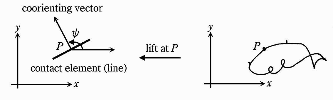
Figure 14. Contact element.

Definition 5.2.

(coorientation) The coorientation of a contact element is the choice of the half-plane into which the contact element divides the tangent plane (Figure 14).

The manifold $M$ consisting of all of the contact elements in the plane is diffeomorphic to solid torus. Consider immersion : $S^{1}\to M$. For each element of this curve in the plane, the coorient of the element is determined (Figure 14). This curve which is Legendrian submanifold of $M$ is called Legendrian curve, the image of projection to plane of this curve is called a front.

By using the following several concepts: elementary move (Definition 5.7), index (Definition 5.5), and Maslov index (Definition 5.6), a front is regarded as a plane curve generated by $K_{i,k}$ (Figure 15) via elementary moves because Theorem 5.1 is established.

$2k$ cusps        $i-1$ kinks    $2k$ cusps

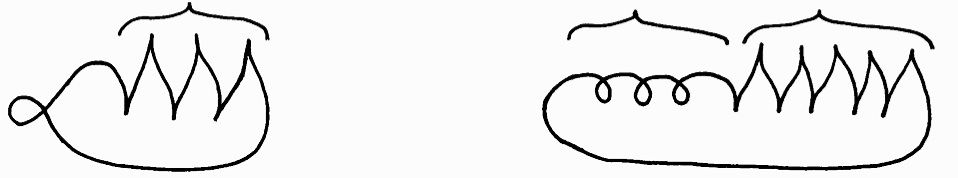
$K_{0,k}$              $K_{i,k}$

Figure 15. Base fronts $\{K_{i,k}\}.$

Let the alphabet $\alpha_{*}$, the involutions $\tau_{1}$, and $\tau_{2}$, the set $S_{*}$ be

$$\alpha_{*} = \{a_{+},a_{-},b_{+},b_{-}\},$$

$$\tau_{1} : a_{+}\mapsto b_{+},a_{-}\mapsto b_{-},$$

$$\tau_{2} : a_{+}\mapsto b_{-},a_{-}\mapsto b_{+},$$

$$S_{*} = \{(a_{\epsilon},a_{\eta},a_{\xi}),(b_{\epsilon},b_{\eta},b_{\xi}):\epsilon,\eta,\xi=+,~{}{\rm or}~{}-\}.$$

(They are different from the involution $\tau$, $S_{*}$ for $\alpha_{*}$ in [Tu4]. )

To the following relations

$$a_{+}+b_{+}=0,\quad a_{-}+b_{-}=0$$

are established, we consider the ring $\overline{\mathbf{Q}\tilde{\alpha_{*}}}$ into which two-sided ideal generated by $a_{+}+b_{+}$ , $a_{-}+b_{-}$ divides the monoid algebra $\mathbf{Q}\tilde{\alpha_{*}}$ where $\tilde{\alpha_{*}}$ is commutative monoid generated by $\alpha_{*}\cup\{1\}$.

Remark 5.1.

If we regard $a_{+}$, $b_{+}$, $\tau_{1}$ in the same light as $a$, $b$, $\tau$ the discussion from Sect. 2 to Sect. 4 still holds on this establishment because $a_{-}$, $b_{-}$, $\tau_{2}$ do not appear Sect. 2, 3, and 4. That is to say, this establishment is canonical generalization of the establishment in Sect. 2, 3, and 4.

From this section, we denote by $|~{}|$ projection $:$ $\mathcal{A}\to\alpha_{*}.$

Definition 5.3.

($|A|$ corresponding to a double point) We define $|A|$ corresponding to a double point $A$ by Figure 16.

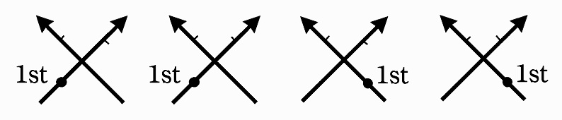
$a_{+}$     $a_{-}$     $b_{+}$      $b_{-}$

Figure 16. Correspondence 4 patterns of double points to 4 alphabets.

Definition 5.4.

($|K|$ corresponding to a cusp) $|K|$ where $K$ is a cusp is defined by Figure 17.

$a_{+}$       $a_{-}$      $b_{+}$       $b_{-}$

Figure 17. Correspondence 4 patterns of cusps to 4 alphabets.

Definition 5.5.

(index) Index of a front $F$ is the number of the full rotations of the coorienting normal vector counter clockwise while we trip along the front once.

Definition 5.6.

(Maslov index) For étale word $(\mathcal{A}_{F},w_{F})$ of front $F$, let $K$ is a letter of $\mathcal{A}_{F}$ for a cusp. Maslov index $\mu$ is defined by

$$\mu=card\{K\in\mathcal{A}_{F}||A|=a_{+}~{}{\rm or}~{}b_{+}\}-card\{K\in\mathcal{A}_{F}||A|=a_{-}~{}{\rm or}~{}b_{-}\}.$$

The local moves of fronts (Figure 18, Figure 19, Figure 20, Figure 21, Figure 22) is defined by the following. Suppose the local moves are admitted apart from base point.

Definition 5.7.

(elementary move of fronts) Let $x$, $y$, $z$ be words that consist of the letter in $\mathcal{A}$. Four kinds of elementary move $I\!I$ are defined by

$$S\!I\!I^{+}:(\mathcal{A}\cup\{A,B\},xAByABz)\to(\mathcal{A},xyz)~{}\text{with}~{}\tau_{1}(|A|)=|B|,$$

$$S\!I\!I^{-}:(\mathcal{A},xyz)\to(\mathcal{A}\cup\{A,B\},xAByBAz)~{}\text{with}~{}\tau_{1}(|A|)=|B|,$$

$$D\!I\!I^{+}:(\mathcal{A},xyz)\to(\mathcal{A}\cup\{A,B\},xAByABz)~{}\text{with}~{}\tau_{1}(|A|)=|B|,$$

$$D\!I\!I^{-}:(\mathcal{A}\cup\{A,B\},xAByBAz)\to(\mathcal{A},xyz)~{}\text{with}~{}\tau_{1}(|A|)=|B|.$$

Let $x$, $y$, $z$, t be words that consist of the letter in $\mathcal{A}-\{A,B,C\}$.

elementary move $I\!I\!I$ is defined by

$$I\!I\!I:(\mathcal{A},xAByACzBCt)\to(\mathcal{A},xBAyCAzCBt)~{}\text{for}~{}(|A|,|B|,|C|)\in S_{*}.$$

Let $x$, $y$, $z$ be words that consist of the letter in $\mathcal{A}-\{K\}$.

Two kinds of elementary move $\Pi$ is defined by

$$\qquad\quad\Pi^{+}:(\mathcal{A},xKyz)\to(\mathcal{A}\cup\{A,B\},xAKByABz)\qquad\qquad\qquad\qquad\qquad\qquad\qquad$$

$$\text{or}~{}(\mathcal{A},xKyz)\to(\mathcal{A}\cup\{A,B\},xAByAKBz)~{}\text{with}~{}\tau_{2}(|A|)=|B|,\qquad$$

$$\qquad\quad\Pi^{-}:(\mathcal{A}\cup\{A,B\},xAKByBAz)\to(\mathcal{A},xKyz)\qquad\qquad\qquad\qquad\qquad\qquad\qquad$$

$$\text{or}~{}(\mathcal{A}\cup\{A,B\},xAByBKAz)\to(\mathcal{A},xKyz)~{}\text{with}~{}\tau_{2}(|A|)=|B|.$$

Let $x$, $y$ be words that consist of the letter in $\mathcal{A}.$ elementary move $\Lambda$ is defined by

$$\Lambda:(\mathcal{A},xy)\to(\mathcal{A}\cup\{A,K_{1},K_{2}\},xAK_{1}K_{2}Ay)~{}\text{with}~{}\tau_{1}\circ\tau_{2}(|K_{1}|)=|K_{2}|.$$

The positive elementary moves is the above direction, negative is the inverse direction.

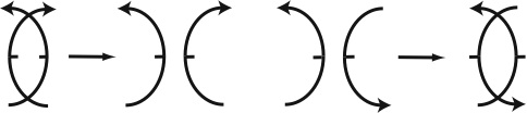
Figure 18. Elementary move $S\!I\!I^{+}$ (left figure), $S\!I\!I^{-}$ (right figure).

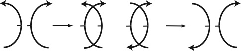
Figure 19. Elementary move $D\!I\!I^{+}$ (left figure), $D\!I\!I^{-}$ (right figure).

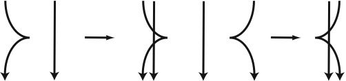
Figure 20. Elementary move $\Pi^{+}$.

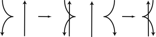
Figure 21. Elementary move $\Pi^{-}$.

Figure 22. Elementary move $\Lambda$.

Remark 5.2.

$S\!I\!I$ stands for safe 2-move,and $D\!I\!I$ means dangerous 2-move (2-move, 3-move resemble Reidemeister move $I\!I$, $I\!I\!I$). In the lift of the plane, self-tangency under dangrous move is corresponded to crossing of the Legendrian curve (cf. [Ai2]).

We have the next theorem due to Gromov [Gr].

Theorem 5.1.

(Gromov) Any front whose index is $i$, Maslov index is $2k$ is deformed via $D\!I\!I^{+}$, $D\!I\!I^{-}$, $S\!I\!I^{+}$, $S\!I\!I^{-}$, $I\!I\!I$, $\Pi^{+}$, $\Pi^{-}$, $\Lambda$ from $K_{i,k}$ (Figure 15).

The object of this section is giving a classification of fronts more detail than the classification by Theorem 5.1. To do this, we consider an application a method like Sect. 3, 4 to front which may have not only double points but also cusps. We consider only double points and cusps due to Theorem 5.1.

We get following theorem.

Theorem 5.2.

All fronts are represented as étale words.

Proof.

For an arbitrary given front which has precisely $n$ double points and precisely $m$ cusps, we name double points $A_{1},A_{2},\ldots,A_{n}$ and name cusps $K_{1},K_{2},\ldots,K_{m}$ along front from the base point. Every double point and every cusp precisely corresponds to a unique element of $\alpha_{*}$ in Figure 16. ∎

5.2. The basic invariants of fronts

The basic invariants of fronts $J^{+},J^{-},St$ are three invariants can be defined as follows (cf. [Ar2], [P]).

Definition 5.8.

$J^{+}$ is increased by $2$ under positive elementary move $D\!I\!I^{+}$, $D\!I\!I^{-}$ but not change under the other,

$J^{-}$ is decreased by $2$ under positive elementary move $S\!I\!I^{+}$, $S\!I\!I^{-}$ but not change under the other,

$St$ is increased by $1$ under positive elementary move $I\!I\!I$, increased by $\frac{1}{2}$ under positive elementary move $\Pi^{+}$, and decreased by $\frac{1}{2}$ under positive elementary move $\Pi^{-}$, but not change under the other, and satisfy the following conditions

$$J^{+}(K_{0,k})=-k,\quad J^{-}(K_{0,k})=-1,\quad St(K_{0,k})=\frac{k}{2},$$

$$J^{+}(K_{i+1,k})=-2i-k,\quad J^{-}(K_{i+1,k})=-3i,\quad St(K_{i+1,k})=i+\frac{k}{2}$$

for the base curves $\{K_{i}\}$ defined by Figure 15.

5.3. Construction of invariants $FI_{n}$

In this subsection we will construct invariants of fronts.

Definition 5.9.

(fake Gauss word) We call a word $w$ a fake Gauss word of dimension $n$ if $w^{\prime}:2m\to\mathcal{A}$ is a Gauss word where $w^{\prime}$ is a sub-word of $w$ and $\{w(1),w(2),\ldots,w(2m)\}$ $\sqcup$ $\{K_{1},K_{2},\ldots,K_{2l}\}$ $=$ $\{w(1),w(2),\ldots,w(2(m+l))\}$ where $n=m+2l$.

Definition 5.10.

(fake nanoword) An étale word $(\mathcal{A},w)$ over $\alpha_{*}$ is a fake nanoword over $\alpha_{*}$ of dimension $n$ if $(\mathcal{A},w)$ satisfies $(\mathcal{A}-\{K_{1},K_{2},\ldots,K_{2l}\},w^{\prime})$ is an nanoword over $\alpha_{*}$ where the length of $w$ is $card\mathcal{A}^{\prime}+2l=n$ and $w^{\prime}$ is a sub-word of $w$.

Remark 5.3.

We can consider a front $F$ on a surface which is a curve on a surface with coorientation and cusps. A fake nanoword gives rise to a nanoword $w$ by neglecting letters for cusps. We can calculate the genus $g(F)$ of a surface on which a fronts because $g(F)$ is equal to $g(\Gamma)$ where $\Gamma$ is determined by the nanoword $w$ by using Theorem 2.2.

Definition 5.11.

(fake word space) The fake word space of degree $n$ is the word space generated by fake Gauss words of dimension $n$.

In 5.3 and 5.4, suppose fake Gauss word, fake nanoword and fake word space are made of only $1$-dimensional letters. We denote by $FW_{n}$ the fake word space is made of fake Gauss words such that all letters are $1$-dimensional letters.

Let $\epsilon$ be $\epsilon=+,~{}\text{or}~{}-$. For every $A\in\alpha_{*}$-alphabet $\mathcal{A}$, $\mathit{sign}(|A|)$ is $1$ if $|A|=b_{\epsilon}$ and $\mathit{sign}(|A|)$ is $-1$ if $|A|=a_{\epsilon}$ (We consider its generalization in Sect. 6). Let $w_{F}$ stand for a word which is determined by a front $F$. By using Theorem 2.3, for every pointed front (which means every front with a base point), the following $\{FI_{n}\}$ is plane isotopy invariants sequence.

$$FI_{n}(F)=\left\langle\sum_{k}x_{k}v_{k},w_{F}\right\rangle\qquad(n\in\mathbf{N}).$$

${v_{k}}$ is a sequence consisting of all elements in $FW_{n}$, and each $x_{k}$ is a parameter.

In the same way of Sect. 3.2, in order to simplify following description, we define proper equivalent classes of fake nanowords over $\alpha_{*}$.

Definition 5.12.

(cyclic equivalent for fronts) Let $w(2)\cdots w(n)$ of $w=w(1)w(2)\cdots w(n)$ represent $x$, for two arbitrary $w,w^{\prime}\in FW_{n}$, relation $\sim$ is defined by

$$w\sim w^{\prime}\stackrel{{\scriptstyle def}}{{\Longleftrightarrow}}\left\{\begin{array}[]{ll}w=Ax~{}\text{and}~{}w^{\prime}=-xA&\text{if~{}A means a double point}\\ w=Kx~{}\text{and}~{}w^{\prime}=xK&\text{if~{}when K means a cusp}\\ \end{array}\right.$$

This relation $\sim$ is called the cyclic equivalent for fronts.

Corollary 5.1.

The cyclic equivalent for fronts is equivalent relation.

Let $\overline{FW}_{n}$ be a module consisting of cyclic equivalent classes for front and $FN_{d}$ the $\mathbf{Q}$-module generated by the set of fake nanoword over $\alpha_{*}$ $\{(\mathcal{A},w)\}$ such that $card\mathcal{A}$ is less than $d+1$.

The mapping $\left[,\right]:\overline{FW}_{n}\times FN_{d}\to\mathbf{Q}$ is defined by

$$\left[[v],w\right]:=\left<v_{1}+v_{2}+\cdots+v_{2l},w_{F}\right>,$$

$v_{1},v_{2},\ldots,v_{2l}$consist of all elements of $[v]$.

Proposition 5.1.

For every $[w]$ which is one of base of $\overline{FW}_{n}$, $[[w],w_{F}]$ is an invariant of curve $\Gamma$.

Proof.

The proof is similar to the proof of Proposition 3.1. ∎

5.4. $FI_{2}$ and $FI_{3}$

For every front $F=(\mathcal{A}_{F},w_{F})$, let $i$ be index and $2c$ the number of cusps,

$$n_{\epsilon}=card\{A\in\mathcal{A}_{F}:|A|=a_{\epsilon}~{}\text{or}~{}b_{\epsilon}\}~{}(\epsilon=+,\text{or}~{}-).$$

We define $FI_{2}$ by

$$FI_{2}(F;p,q,r,s,t,u,v) := pn_{+}+qn_{-}+\langle rXXYY-rXYYX+sXYXY$$

$$+tKXX+tXXK-tXKX+uKK,w_{F}\rangle+vc$$

$$+\frac{r}{2}-\frac{r}{2}i^{2}.$$

$FI_{2}$ is also not depend on the orientation of each front $F$ because this formula is symmetric.

Theorem 5.3.

$FI_{2}$ is an invariant which is stronger than$(J^{+},J^{-},St)$.

$i.e.$ For a front $F$, $FI_{2}(F)$ is not depend on the choice of the base point, for two arbitrary fronts $F_{1}$, $F_{2}$,

$$FI_{2}(F_{1})=FI_{2}(F_{2})\Longrightarrow(J^{+}(F_{1}),J^{-}(F_{1}),St(F_{1}))=(J^{+}(F_{2}),J^{-}(F_{2}),St(F_{2})),$$

and the converse can not be established.

Proof.

(I) First, we will prove that for an arbitrary front $F$, $FI_{2}(F)$ is not depend on the choice of a base point. Base point move (Figure 24) means $x,y$ is word consisting of letters in $\mathcal{A}-\{A\}$, in the case of $A$ is a double point, as Proposition 3.1, $(\mathcal{A},w_{F})=AxAy\to xA_{\tau}yA_{\tau},|A_{\tau}|=\tau_{1}(|A|),$ in the case of $A$ is a cusp $i.e.A=K$, $(\mathcal{A},w_{F})=Kxy\to xyK,|K|$ is not change .

$\left\langle XXYY-XYYX,w_{F}\right\rangle,\left\langle XYXY,w_{F}\right\rangle$ is not depend on the choice of a base point due to [P].

Therefore to prove it is checking increase and decrease of only the terms

$$\left\langle tKXX+tXXK-tXKX,w_{F}\right\rangle$$

under an arbitrary base point move.

(I​I) For front $F_{1}$, $F_{2}$,

$$FI_{2}(F_{1})=FI_{2}(F_{2})\Longrightarrow(J^{+}(F_{1}),J^{-}(F_{1}),St(F_{1}))=(J^{+}(F_{2}),J^{-}(F_{2}),St(F_{2})),$$

and the converse can not be established.

($\Longrightarrow$). The following three relations are concluded by Polyak in [P].

$$J^{+}(F) = FI_{2}(F;-\frac{1}{2},-\frac{3}{2},1,-3,\frac{1}{2},\frac{1}{4},-\frac{3}{4}),$$

$$J^{-}(F) = FI_{2}(F;-\frac{3}{2},-\frac{1}{2},1,-3,\frac{1}{2},\frac{1}{4},\frac{1}{4}),$$

$$St(F) = FI_{2}(F;\frac{1}{4},\frac{1}{4},-\frac{1}{2},\frac{1}{2},-\frac{1}{4},-\frac{1}{8},\frac{3}{8}).$$

( $\Longleftarrow$ can not be established. ) There exists counterexample : Figure 23.

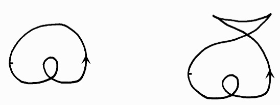
Figure 23. The values of basic invariants of two fronts are same, but the value of $FI_{2}$ of one of them is different from that of another.

∎

Figure 24. Base point move.

Remark 5.4.

There is a relation $J^{+}-J^{-}=n_{+}-n_{-}-c$ (cf. [P]).

We will consider application $I_{3}$ to fronts.

Let $i$ be index. For every front $F$, we define $FI_{3}$ by

$FI_{3}(F;x,y,z,p,q,r,s,t):=CI_{3}(F;x,y,z)+\Big{[}p[XKXYY]+q[KXXYY]\newline +r[XKYXY]+s[XXKK]+t[KKK],w_{F}\Big{]}.$

Theorem 5.4.

$FI_{3}$ is an invariant of fronts.

Proof.

To prove this, we must prove that $FI_{3}(F)$ is independent of base point move (Figure 24) for every front, but it is immediately concluded by Proposition 5.1. ∎

Corollary 5.2.

Suppose $-F$ has only difference of orientation from $F$, and let $F^{r}$ be the reflection of $F$,

$$FI_{3}(-F)=-FI_{3}(F),\quad FI_{3}(F^{r})=-FI_{3}(F).$$

Remark 5.5.

$FI_{2}(-F)=FI_{2}(F)$.

The following is example of the pair of curves such that the values of index, Maslov index, the basic invariants, and $FI_{2}$ are the same, but the value of $FI_{3}$ on one front is different from that on the other.

Example 5.1.

There exist two curves (Figure 25), such that $($$i,$ $\mu,$ $J^{+},$ $J^{-},$ $St,$ $FI_{2}$$)$ $=$ $($$1,$ $2,$ $-3,$ $-4,$ $6,$ $2p$ $-$ $r$ $-$ $u$ $+$ $v$$)$ and the values of one front is different from another.

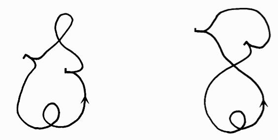
Figure 25. Two fronts such that $($$i,$ $\mu,$ $J^{+},$ $J^{-},$ $St,$ $FI_{2}$$)$ $=$ $($$1,$ $2,$ $-3,$ $-4,$ $6,$ $2p$ $-$ $r$ $-$ $u$ $+$ $v$$)$. The value of $FI_{3}$ is $2s+1$ for left figure, $2s-4p+1$ for right figure.

5.5. Strengthening $FI_{n}$

In this section, suppose fake Gauss word (Definition 5.9), fake nanoword (Definition 5.10), and fake word space (Definition 5.11) are made of not only $1$-dimensional letters but also $2$-dimensional letters. We can strengthen $FI_{n}$ by the similar method of Sect. 2.3, 3.4, 4.4. We must define marked cyclic equivalent for fronts which is the canonical generalization of cyclic equivalent for fronts defined in Sect. 5.3.

In distinction from $FW_{n}$, we denote by $\mathcal{FW}_{n}$ the fake word space may have fake Gauss words which letters are not only $1$-dimensional letters but also $2$-dimensional letters.

Definition 5.13.

(marked cyclic equivalent for fronts) Let $w(2)\cdots w(n)$ of $w=w(1)w(2)\cdots w(n)$ represent $y$, for two arbitrary $w,w^{\prime}\in\mathcal{FW}_{n}$, relation $\sim$ is defined by

$$w\sim w^{\prime}\stackrel{{\scriptstyle def}}{{\Longleftrightarrow}}\left\{\begin{array}[]{lll}\text{when X means a double point,}&w=Xy~{}\text{and}~{}w^{\prime}=-yX&\text{if}~{}d(X)=1\\ &w=\dot{X}y~{}\text{and}~{}w^{\prime}=y\dot{X}&\text{if}~{}d(X)=2\\ \text{when K means a cusp,}&w=Ky~{}\text{and}~{}w^{\prime}=yK&\text{if}~{}d(K)=1\\ &w=\dot{K}y~{}\text{and}~{}w^{\prime}=y\dot{K}&\text{if}~{}d(K)=2\end{array}\right.$$

This relation $\sim$ is called marked cyclic equivalent for fronts.

Replacing cyclic equivalent for fronts by marked cyclic equivalent for fronts, we can easily check that the similar results are established and can easily generalize Sect. 5.4. Therefore we only see the case of $FI_{3}$. Let $i$ be index. For every front $F$, we define $GFI_{3}$ by

$GFI_{3}(F;x,y,z,p,q,r,s,t,u,v,h):=GCI_{3}(F;x,y,z)+\Big{[}p[XKXYY]+q[KXXYY]\\ +r[XKYXY]+s[KKK]+t[XXKK]+u[\dot{K}XX]+v[K\dot{X}\dot{X}]+h[\dot{K}K],w_{F}\Big{]}.$

Corollary 5.3.

$GFI_{3}$ is an invariant of fronts.

Example 5.2.

There exist two fronts such that the value of $FI_{3}$, index, Maslov index, basic invariants are the same; however, the value of $GFI_{3}$ on one curve is different from that on the other (Figure 26).

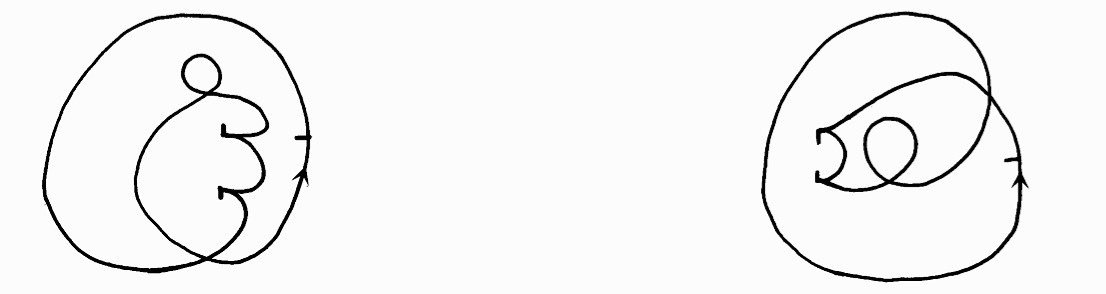
Figure 26. Two fronts such that $($$FI_{3},$ $i,$ $\mu,$ $J^{+},$ $J^{-},$ $St$$)$ is $($$2q+2,$ $2,$ $0,$ $-4,$ $-5,$ $2$$)$. The value of $GFI_{3}$ is $2q-2u+2v+2$ for the left figure, $2q+2u+2$ for the right figure.

In particular, this example implies the following.

Corollary 5.4.

$GFI_{3}$ is a stronger invariant than $FI_{3}.$

6. Generalization

By replacing the function $\mathit{sign}$ with $\rho$, we get more general invariants.

6.1. Generalization of $I_{n}$

Let $\tilde{\alpha}$ be commutative monoid generated by an alphabet $\alpha$ which contains the unit element and consider monoid algebra $\mathbf{Q}\tilde{\alpha}$. For every $A\in\alpha$-alphabet $\mathcal{A}$ , suppose mapping $\rho:|A|\to\rho(|A|)\in\mathbf{Q}\tilde{\alpha}$ is given.

When an arbitrary étale word $w$ is given, choose a sub-word $v$ of $w$, for this sub-word $v$, sub-étaleword $(\mathcal{A}_{v},v)$ of $w$ is determined , and then

$$\rho(v):=\prod_{A\in{A_{v}}}\{\rho(|A|)\}^{d(A)}$$

can be defined. By using this, for every étale word $w$ and every sub-word $v$ of $w$, we define the mapping

$$\left\langle v,w\right\rangle:=\sum_{\text{a sub-word $v^{\prime}$ of $w$ isomorphic to $v$}}\rho(v^{\prime}).$$

Let $W_{n}$ be the $\mathbf{Q}$-module generated by the set of all of the fake-Gauss words in $FW_{n}$. Let $FN_{d}$ be the free $\mathbf{Q}$-module generated by the set of fake nanowords over $\alpha$ $\{(\mathcal{A},w)\}$ such that $card\mathcal{A}$ is less than $d+1.$ Expanding $\left\langle v,w\right\rangle$ bilinearly, we can make a bilinear mapping$\left\langle,\right\rangle$ from $FW_{n}\times FN_{d}$ to $\mathbf{Q}.$ For an arbitrary surface, let $w_{\Gamma}$ stand for a word which is determined by a curve $\Gamma$ on the surface.

Theorem 6.1.

The following $\{\tilde{I}_{n}\}$ (invariant of degree $n$) is the sequence of surface isotopy invariants for pointed curves on a surface.

$$\tilde{I}_{n}(\Gamma)=\left\langle\sum_{k}x_{k}v_{k},w_{\Gamma}\right\rangle\qquad(n\in\mathbf{N})$$

where $\{v_{k}\}$ is the basis of $W_{n}$ and each $x_{k}$ is a parameter.

Proof.

Theorem 2.3 and the construction of $\langle,\rangle$ deduce immediately this theorem. ∎

6.2. Investigation of the generalization in the case $FI_{2}$

For example, we will consider the case $FI_{2}$, and so we get an invariant $\widetilde{FI_{2}}$ which is stronger than $FI_{2}$. For every element $A\in\alpha_{*}$-alphabet $\mathcal{A}$, $\rho$ is defined by $\rho(|A|)=|A|\in\overline{\mathbf{Q}\tilde{\alpha_{*}}}$.

Let $F$ be front. By using the construction of $\left[,\right]$, the following $\widetilde{FI_{n}}$ is a plane isotopy invariant of fronts.

$$\widetilde{FI_{n}}(F)=\left[\sum_{i,j}x_{j}[v_{i}],w_{F}\right]\qquad(n\in\mathbf{N}).$$

$[v_{i}]$ in $\overline{FW}_{n}$ (cf. Proposition 5.1), each $x_{j}$ is a parameter.

For front $F=(\mathcal{A}_{F},w_{F})$, let $i$ be index, $2c$ the number of cusps,

$$n_{\epsilon}=card\{A\in\mathcal{A}_{F}:|A|=a_{\epsilon}~{}\text{or}~{}b_{\epsilon}\}~{}(\epsilon=+,~{}\text{or}~{}-).$$

We define $\widetilde{FI_{2}}$ by

$$\widetilde{FI_{2}}(F;p,q,x,z,t,v,r) := pn_{+}+qn_{-}+\langle xXXYY-xXYYX+zXYXY$$

$$+tKXX+tXXK-tXKX+vKK,w_{F}\rangle+rc$$

$$+\frac{x}{2}-\frac{x}{2}i^{2}.$$

Theorem 6.2.

$\widetilde{FI_{2}}$ is an invariant which is stronger than $FI_{2}$.

Proof.

The value of $FI_{2}$ is obtain from $\widetilde{FI_{2}}$ by regarding $a_{+}$, $a_{-}$ as $1$. Therefore $\widetilde{FI_{2}}$ is at least as strong as $FI_{2}$. So, Figure 27 deduces that $\widetilde{FI_{2}}$ is an invariant which is stronger than $FI_{2}$.

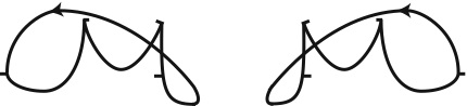
Figure 27. The values of $FI_{2}$ for these two fronts are $p$ $+q$ $+x$ $+2t$ $-v$ $+2r$. The values of $\widetilde{FI_{2}}$ for left figure is $p+q+(-\frac{3}{2}+a_{+}a_{-})x+({a_{-}}^{2}+{a_{+}}^{2})t+(a_{+}a_{-})v+2r$, The values of $FI_{2}$ for right figure is $p+q+(-\frac{3}{2}+a_{+}a_{-})x+({a_{+}}^{2}+2a_{+}a_{-}-{a_{-}}^{2})t+(a_{+}a_{-})v+2r$.

∎

Remark 6.1.

Suppose let $F^{r}$ be the reflection of $F$, and then $\widetilde{FI_{2}}(F)=\widetilde{FI_{2}}(F^{r})$. On the other hand, suppose $-F$ has only the difference of orientation from $F$, and then there exists an example (left figure in Figure 27) as $\widetilde{FI_{2}}(F)\neq\widetilde{FI_{2}}(-F)$ (cf. $CI_{2}$, $LI_{2}$).

Remark 6.2.

For these two fronts, $(i,\mu,J^{+},J^{-},St)=(2,0,-2,-1,2)$, and in terms of invariants of fronts : $f^{+},f^{-},p^{\uparrow},p^{\downarrow},\lambda^{\uparrow},\lambda^{\downarrow}$ due to Aicardi [Ai1], $($$f^{+},$ $f^{-},$ $p^{\uparrow},$ $p^{\downarrow},$ $\lambda^{\uparrow},$ $\lambda^{\downarrow}$$)$ $=$ $($$2,$ $0,$ $-2,$ $0,$ $2,$ $0$$)$.

Remark 6.3.

$\widetilde{FI_{2}}$ is the deformation $\overline{FI_{2}}$. Moreover, because $\left\langle\dot{X}\dot{X},w_{F}\right\rangle=n_{+}{a_{+}}^{2}+n_{-}{a_{-}}^{2}$, if the term $\left\langle\dot{X}\dot{X},w_{F}\right\rangle$ is taken place of $n_{+}p+n_{-}q$, the strength of the invariant does not change.

Department of Mathematics and Applied Mathematical Science Sciences

Graduate School of Fundamental Science and Engineering

Waseda University

3-4-1 Okubo, Shinjyuku-ku

Tokyo 169-8555, JAPAN

email: noboru@moegi.waseda.jp

References

- [Ar1] V. I. Arnold, Plane curves, their invariants, perestroikas and classifications, Advances in Soviet Mathematics, AMS 21, Providence (1994), 33–91.
- [Ar2] V. I. Arnold, Topological invariants of plane curves and caustics, University Lecture Series 5, Providence, RI, 1994.
- [Ar3] V. I. Arnold, Invariants and perestroikas of plane fronts, Proc. Steklov Inst. Math. 209 (1995), 11–56.
- [Ai1] F. Aicardi, Discriminants and local invariants of planar fronts, The Arnold-Gelfand mathematical Seminars, Birkhäuser Boston, Boston, MA (1997), 1–76.
- [Ai2] F. Aicardi, Invariant polynomial of framed knots in the solid torus and its application to wave fronts and Legendrian knots, Journal of Knot Theory and Its Ramifications, 5 (1996), 743–778.
- [CGM] S. Chumutov, V. Goryunov, H. Murakami, Regular Legendrian knots and the HOMFLY polynomial of immersed plane curves, Math. Ann. 317 (2000), 389–413.
- [Gr] M. Gromov, Partial differential relations, Springer-Verlag. Berlin and New York, 1986.
- [GN] S. M. Gusein-Zade, S. M. Natanzon, The Arf-invariant and the Arnold invariants of plane curves, The Arnold-Gelfand mathematical Seminars, Birkhäuser Boston, Boston, MA (1997), 267–280.
- [P] M. Polyak, Invariants of curves and fronts via Gauss diagrams, Topology 37 (1998), 989–1009.
- [Tc] V. Tchernov, Arnold-type invariants of wave fronts on surfaces, Topology 41 (2002), 1–45.
- [Tu1] V. Turaev, Curves on surface, charts, and words, Geometriae Dedicata 116 (2005), 203–236.
- [Tu2] V. Turaev, Virtual strings, Ann. Inst. Fouruer 54 7 (2004), 2455-2525.
- [Tu3] V. Turaev, Topology of words, math.CO/0503683.
- [Tu4] V. Turaev, Knots and words, math.GT/0506390.
- [Tu5] V. Turaev, Lectures on topology of words, RIMS-1567 (2006).
- [Va] V. A. Vassilliev, Cohomology of knot spaces, Theory of singularities and its applications, Adv. Soviet Math. 1, Amer. Math. Soc. , Providence, RI (1990), 23–69.
- [Vi] O. Viro, Virtual links, Orientations of chord diagrams and Khovanov homology, Proceedings of Gk̈ova Geometry-Topology Conference (2005), 184–209.
- [W] H. Whitney, On regular closed curves in the plane, Compositio Math. 4 (1937), 276–284.
- [ZZP] J. Zhou, J. Zou, J. Pan, The basic invariants of long curve and closed curve perestroikas, Journal of Knot Theory and Its Ramifications, 7 (1998), 527–548.