Non-saturating magnetoresistance of inhomogeneous conductors: comparison of experiment and simulation

Abstract

The silver chalcogenides provide a striking example of the benefits of imperfection. Nanothreads of excess silver cause distortions in the current flow that yield a linear and non-saturating transverse magnetoresistance (MR). Associated with the large and positive MR is a negative longitudinal MR. The longitudinal MR only occurs in the three-dimensional limit and thereby permits the determination of a characteristic length scale set by the spatial inhomogeneity. We find that this fundamental inhomogeneity length can be as large as ten microns. Systematic measurements of the diagonal and off-diagonal components of the resistivity tensor in various sample geometries show clear evidence of the distorted current paths posited in theoretical simulations. We use a random resistor network model to fit the linear MR, and expand it from two to three dimensions to depict current distortions in the third (thickness) dimension. When compared directly to experiments on $\mathrm{Ag}_{2\pm\delta}\mathrm{Se}$ and $\mathrm{Ag}_{2\pm\delta}\mathrm{Te}$, in magnetic fields up to 55 T, the model identifies conductivity fluctuations due to macroscopic inhomogeneities as the underlying physical mechanism. It also accounts reasonably quantitatively for the various components of the resistivity tensor observed in the experiments.

I Introduction

Macroscopic inhomogeneities were generally associated with a diminution of galvanomagnetic effects, due to the reduction of carrier mobility caused by impurity scattering. Classical effective media theories 1 ; 2 ; 3 ; 4 ; 5 ; 6 ; 7 ; 8 have shown, on the other hand, that conductors normally exhibiting no change in resistance $R$ when a magnetic field $H$ is applied, can possess a positive magnetoresistance, $\Delta R/R\equiv(R(H)-R(0))/R(0)$, in the presence of spatial fluctuations of the resistivity, provided that the characteristic length scale of the inhomogeneity is much larger than the mean free path. This induced magnetoresistance depends generically on whether the magnetic field is oriented perpendicular (transverse MR) or parallel (longitudinal MR) to the current direction. In recent experiments, Solin and co-workers 9 ; 10 have harnessed this effect by crafting composite materials in which current deflections around highly conducting inhomogeneities significantly enhance the intrinsic transverse MR of $\mathrm{Hg}_{1-x}\mathrm{Cd}_{x}\mathrm{Te}$. This designer approach depends on the mismatch in the physical MR of the two components and leads to a significant, quadratic magnetoresistance that saturates by $H\sim$ 0.5 T.

In addition to geometric enhancements to the galvomagnetic response of materials with intrinsic physical MR, there is the possibility of designing materials and devices where the MR arises solely from the macroscopic inhomogeneities. In such a case, where the disorder-induced component of the magnetoresistance can be separated from the physical magnetoresistance, the functional form of the MR not only can be tuned to be linear with magnetic field, but it is possible to craft a response that continues to at least a MegaGauss. Essential design considerations involve the pertinent inhomogeneity length scale, which can involve both the dopant distribution and polycrystalline structure, adjacency to a zero band gap condition to amplify the effects of fluctuations in the carrier mobilities, and the ease of growth and fabrication.

The silver chalcogenides stand out as favorable materials for the investigation of large, linear and non-saturating MR because of their simplicity and tunability. Perfectly stoichiometric $\mathrm{Ag}_{2}\mathrm{Se}$ and $\mathrm{Ag}_{2}\mathrm{Te}$ are non-magnetic, narrow-gap semiconductors whose electron and hole bands cross at liquid nitrogen temperatures. They exhibit negligible physical magnetoresistance 11 , as predicted from conventional theories. By contrast, minute amounts of excess Ag or Te/Se $-$ at levels as small as 1 part in 10,000 $-$ lead to a huge and linear magnetoresistance over a broad temperature range, with no sign of saturation up to 60 T 12 ; 13 ; 14 ; 15 ; 16 ; 17 . In particular, the unusual linearity extends deep into the low field regime with $H\ll 1/\mu$, where $\mu$ is the typical mobility of the material. Such behavior shows no resemblance to conventional semiconductors, where the magnetoresistance grows quadratically with field and reaches saturation at fields typically of order 1 T. Therefore, it has been argued that the observed magnetoresistance must be caused by the inhomogeneous distribution of excess/deficient silver ions 18 ; 19 . The spatial inhomogeneities in the silver chalcogenides result from the clustering of Ag ions at lattice defects or grain boundaries when quenched from the high temperature $\alpha$-phase to the semiconducting $\beta$-phase with lower Ag solubility. They may take the form of highly conducting nanothreads or lamellae along the grain boundaries of the polycrystalline material 20 .

Abrikosov was the first to point out the essential role played by inhomogeneities in the magnetoresistance observed in the silver chalcogenides, emphasizing the importance of the zero band gap condition. The phenomenon is quantum in origin and relies on a combination of a linear dispersion and a single, partially-filled Landau band 18 ; 21 . This picture also has been applied to the large, positive MR in epitaxial Bi films 22 and in suitably doped InSb 23 . By contrast, Parish and Littlewood (PL) 19 ; 24 demonstrated that purely classical, geometric effects of the inhomogeneities could be responsible for the non-saturating magnetoresistance in $\mathrm{Ag}_{2\pm\delta}\mathrm{Se}$ and $\mathrm{Ag}_{2\pm\delta}\mathrm{Te}$. They introduced a two-dimensional random resistor network model capable of simulating macroscopic media with complicated boundaries. Their simulations of strongly inhomogeneous semiconductors derive a linear MR from the Hall resistance picked up from macroscopically distorted current paths caused by variations in the stoichiometry. Moreover, when both positive (hole-like) and negative (electron-like) values of the mobility are sampled, as will occur at bank crossing, the functional form of the MR is most linear (consistent with experiments 17 ). The magnetic field scale for the onset of the linear response is then set by the width of the mobility distribution. These results also agree qualitatively with subsequent studies of two-component media involving exact results and effective medium approximations 25 ; 26 ; 27 , which show that the non-saturating transverse magnetoresistance will be maximal when the high field Hall resistance crosses zero.

The exact distribution of inhomogeneities is difficult to resolve via either scattering or imaging techniques for the relevant doping levels in the silver chalcogenides, but the longitudinal MR has been found to serve as an effective probe of the spatial extent of the excess silver nanothreads 28 . The negative longitudinal MR and, in particular, the emergence of an unexpected cross-term in the resistivity tensor coupling the longitudinal and transverse response, appears as a physical manifestation of distorted current paths, with an attendant inhomogeneity length scale. Missing at present, however, is the theoretical depiction of current distortions in the thickness dimension, and the abnormal longitudinal MR associated with it. The majority of theoretical investigations on classical inhomogeneous conductors focus solely on the transverse MR, the major exception being the study of isotropic media with insulating inclusions, where the longitudinal MR is substantially larger than the transverse MR 4 ; 5 . Moreover, the modeling has been restricted to transport properties in the bulk, whereas the presence of boundaries is clearly important for the unusual longitudinal MR of the silver chalcogenides.

In this article, we extend the PL random resistor model to three dimensions in order to permit an explicit comparison to the longitudinal MR results. We find that simple realizations of macroscopic inhomogeneity represent a crucial ingredient for understanding the full magnetoresistive response observed in the experiments. The PL model allows one to simulate the various components of the resistivity tensor, and generate visualizations of the current distortion in the thickness dimension, results only accessible through the computer simulations. Moreover, we test the theory and fix its parameters via direct comparison to the temperature and magnetic field dependence of the transverse MR.

The paper is organized as follows. Section II describes the sample preparation and measurement techniques, while Sec. III reviews both the 2D network model and the 3D expansion we use to visualize the distorted current paths in the presence of a longitudinal magnetic field. In Sec. IV, we compare the simulation results and experimental data regarding the linear transverse magnetoresistance, the transverse-longitudinal coupling $\rho_{xz}(H)$ and the negative longitudinal magnetoresistance. We present our conclusions in Sec. V.

II Experimental Methods

Appropriately weighted amounts of high purity Ag and Te (99.999%, Alfa Aesar) were melted to created polycrystalline $\mathrm{Ag}_{2\pm\delta}\mathrm{Te}$ at desired stoichiometries, both silver rich ($n$-type, $\delta>0$) and silver deficient ($p$-type, $\delta<0$). The compound was ground and loaded into outgassed, fused silica ampoules inside a helium glove box, then baked at 50 K above the melting point (1170 K) to ensure complete mixing. Slowly cooled specimens with typical dimensions (4.0 $\times$ 1.0 $\times$ 0.4) mm³ were cut perpendicular to the cylindrical axis to avoid possible dopant variations due to temperature gradients inside the furnace. $\mathrm{Ag}_{2\pm\delta}\mathrm{Se}$ polycrystals were prepared similarly from stoichiometric $\mathrm{Ag}_{2}\mathrm{Se}$, and appropriate weights of Ag or Se were added to reach the desired compositions. Sample thicknesses from 400 $\mu$m to 15 $\mu$m were obtained by mechanically shaving the same specimen with precise depth control under the microscope.

We performed four-probe magnetotransport measurements using a conventional ac bridge technique in the ohmic and frequency-independent limits. Ultrasonically soldered InBi contacts were placed on the top, bottom and sides of the specimens to determine the $\rho_{xx}$, $\rho_{zz}$ and $\rho_{xz}$ components of the resistivity tensor. The transverse and longitudinal MR was determined by averaging values at positive and negative field directions. The longitudinal MR is much smaller than the transverse MR and thus requires attention to alignment of the magnetic field and current directions (within $\pm 5^{\circ}$). We used a 14/16 T superconducting magnet in a helium-3 cryostat for low field measurements and the 60 T short-pulsed magnet at the National High Magnetic Field Laboratory at Los Alamos for the high field response. The latter provides 16 ms long field pulses from the discharge of a 1 MJ capacitor bank and, when combined with the NHMFL-designed synchronous digital lock-in amplifier with response times much shorter than commercial lock-ins, can provide low noise data during each 16 ms shot.

III Theoretical Models

For classical magnetotransport, where the mean free path of the charge carriers is much less than the typical length scale of the disorder, we can take Ohm’s law to be valid locally in space:

$${\bf E}({\bf r})=\hat{\rho}({\bf r})\ {\bf j}({\bf r}).$$ (1)

Here, $\mathbf{j}$ is the current density, $\mathbf{E}$ is the electric field and $\hat{\rho}$ is the resistivity tensor. For simplicity, we will assume that the inhomogeneities are isotropic and that each point in space is characterized by a single charge carrier, so that the resistivity tensor acquires the following form in a magnetic field $\mathbf{H}=H\hat{z}$:

$$\hat{\rho}\ =\ \rho\left(\begin{array}[]{ccc}1&\beta&0\\ -\beta&1&0\\ 0&0&1\end{array}\right)$$ (2)

Clearly, this tensor is dependent on just two parameters: the carrier mobility $\mu$ (since the dimensionless variable $\beta=\mu H$) and the scalar resistivity $\rho$. A realistic inhomogeneous semiconductor will generally possess multiple charge carriers, but their effect on $\hat{\rho}$ is typically small with $\Delta\rho/\rho\ll 1$ 29 .

In order to address the problem of strong inhomogeneities, PL previously introduced a two-dimensional square network of four-terminal resistor units 19 ; 24 , which we will briefly review here. As shown in Fig. 1(a), the resistor unit is taken to be a homogeneous disk whose transport properties can be calculated easily using Eq. (1). Four terminals are required to take account of the Hall voltage that develops perpendicular to the current direction in a transverse magnetic field. The voltage differences $\nu_{i}$ between terminals are linearly related to the currents $\iota_{j}$ at each terminal via an impedance matrix $z_{ij}$, i.e. $\nu_{i}=z_{ij}\ \iota_{j}$ . Like Eq. (2), the impedance matrix is completely determined by the mobility $\mu$ and an effective scalar resistivity $\rho$. We can thus generate a square $N\times N$ random network (Fig. 1(b)) by connecting up the disks using Kirchoff’s laws and then randomly varying $\mu$ and $\rho$ for each disk. Specifically, we consider the distribution of $\mu$ to be Gaussian with average $\langle\mu\rangle$ and width $\Delta\mu$, while the distribution for $\rho$ must obviously satisfy $\rho\geq 0$ (e.g. we can take $\rho=\eta^{2}$, where $\eta$ has a Gaussian distribution). Note that negative and positive values of $\mu$ correspond to electron-like and hole-like carriers, respectively, and that the case where $\langle\mu\rangle=0$ corresponds to an equal number of electrons and holes since our chosen distribution is symmetric about $\langle\mu\rangle=0$. In order to determine the network resistance $R$, we apply a potential difference $V$ across the network in Fig. 1(b) and then sum up the currents along the left (or right) edge, $I=\sum_{i}^{N}I_{i}^{L(R)}$, so that $R=V/I$. We avoid boundary effects associated with perfectly conducting electrodes on the left and right edges of the network 24 by taking periodic boundary conditions for the currents, $I_{i}^{L}=I_{i}^{R}$.

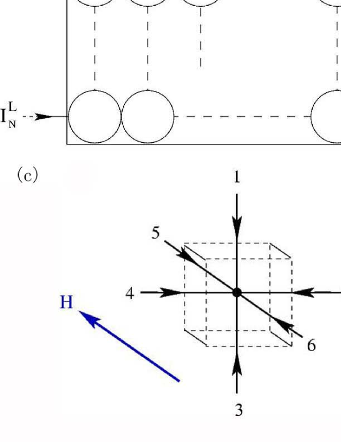
Figure 1: Two-dimensional resistor network model and its extension to three dimensions. The original 2D resistor unit (a) is assumed to be a homogeneous disk with four equally spaced terminals, each of which is associated with a current $\iota_{i}$ and a voltage difference $\nu_{i}$ . The resultant $N\times N$ resistor network (b) has a constant potential difference $V$ applied from left to right, and no current can enter or exit the network at the top and bottom edges. Unlike the previous resistor network model 19 , we assume periodic boundary conditions for the currents on the left and right edges $I_{i}^{L}=I_{i}^{R}$. In the three-dimensional version, the basic unit is naturally a six-terminal element (c) of unit volume, but it now represents a direct discretization of Eq. (1) rather than any particular geometry such as a sphere.

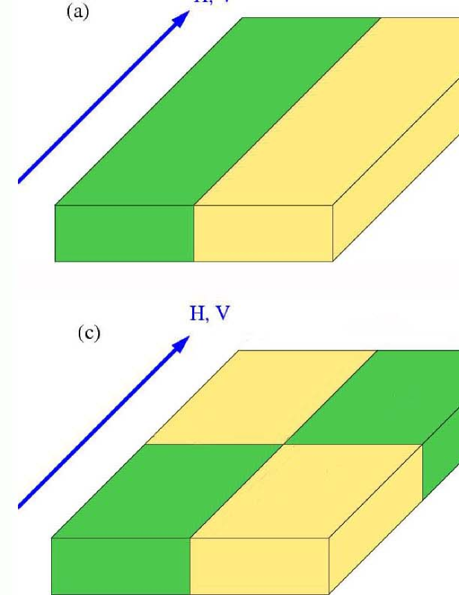
Figure 2: Simple realizations of two-dimensional disorder consisting of two different resistivities $\rho_{1}$ and $\rho_{2}$, where the magnetic field $H$ is parallel to the applied voltage $V$. Patterns (a) and (b) have no longitudinal magnetoresistance, while (c) has a small, saturating one. The magnetoresistance of (d) can be tuned to be large by setting $\rho_{1}/\rho_{2}\gg 1$.

In the limit $N\rightarrow\infty$, this model successfully simulates the transverse MR of an inhomogeneous semiconductor. However, in order to model the longitudinal MR, we must extend this network to three dimensions, even in the case where the inhomogeneity is purely two-dimensional. We should emphasize that there are numerous subtleties associated with adding a third dimension. First, the local resistivity tensor (2) is obviously not isotropic like it is in 2D owing to the fact that there is now a preferred direction along the magnetic field. Indeed, this property is responsible for the standard phenomenon of current jetting 29 . In addition, the resistivity in 3D contains the dimensions of length (i.e. $R=\rho\frac{L_{x}}{L_{y}L_{z}}$) so it is not scale invariant as it is in 2D. From a theoretical standpoint, the extra dimension also makes it impossible to use duality relations 7 ; 8 ; 25 ; 30 or conformal mappings to obtain exact results in 3D, although much progress has been made with effective medium approximations for two-component systems 4 ; 5 ; 6 ; 26 , and by exploiting an analogy with advection-diffusion problems in the continuous, weakly disordered case 2 ; 3 ; 31 .

The above considerations mean that there is no straightforward generalization of the circular resistor unit to 3D. In fact, deceptively trivial geometries like a sphere or a cylinder with its axis perpendicular to the magnetic field have a non-saturating magnetoresistance 32 . Instead, we must employ a “brute-force” approach by directly discretizing Eq. (1) into six-terminal elements as in Ref. 33, and then constructing 3D networks that simulate basic macroscopic inhomogeneities. Referring to Fig. 1(c), we set a voltage and current for each terminal such that each voltage is defined with respect to the element center and incoming currents are defined as positive. The impedance matrix relating voltages and currents is then given by:

$$Z_{ij}=\frac{\rho}{2}(\delta_{ij}+\beta M_{ij})$$ (3)

where

$$\hat{M}=\frac{1}{2}\left(\begin{array}[]{cccccc}0&-1&0&1&0&0\\ 1&0&-1&0&0&0\\ 0&1&0&-1&0&0\\ -1&0&1&0&0&0\\ 0&0&0&0&0&0\\ 0&0&0&0&0&0\end{array}\right)$$ (4)

A major advantage of this model over effective medium approximations is that we can include sample boundaries, a crucial ingredient for understanding the observed negative longitudinal MR in the silver chalcogenides 28 . In particular, we can simulate a four-probe measurement, where the voltage probes placed on top of the sample are separate from the electrodes at the ends of the sample that supply the current (by contrast to the two-probe measurements illustrated in Fig. 2).

The spirit of our investigation will be to construct simple realizations of disorder that capture the salient features of experiment, thereby gaining insight into an otherwise difficult theoretical problem. We depict in Fig. 2 simple examples of possible two-dimensional inhomogeneities with two different resistivities $\rho_{1}$ and $\rho_{2}$. Note that there is no problem with using perfectly conducting electrodes on the ends of the sample, since unlike in a transverse field, there is no contact MR in a longitudinal field. We see straightaway that the classical longitudinal MR of Fig. 2(a) and (b) is zero since all the current is parallel to the potential difference $V$ (or, equivalently, the magnetic field $H$) and is thus insensitive to the Lorentz force. However, once there is a non-zero current perpendicular to the magnetic field, Hall voltages will build up in the $z$-direction, which, in turn, can affect the current flow. The chessboard pattern in Fig. 2(c) exhibits a small magnetoresistance for $\rho_{1}\neq\rho_{2}$ that eventually saturates once the current has found a path across the sample that is parallel to $H$. The ideal pattern is one where the current is forced to flow perpendicular to $H$ and strongly experiences the Lorentz force as in Fig. 2(d) for $\rho_{1}/\rho_{2}\gg 1$. One may even regard this “percolation” pattern as representing a generic filamentary current path analogous to those seen in the 2D network simulations 19 ; 24 , although in this case the current is filamentary even at zero magnetic field. Surprisingly, differences in mobility $\mu$ between the two components have hardly any effect on these simple patterns, so we take $\mu$ to be uniform.

For the remainder of this article, we take Fig. 2(d) to be our basic toy model for longitudinal magnetoresistance. We have computed the magnetoresistance of different $L_{x}\times L_{y}\times L_{z}$ network sizes and we find that it has converged for $L_{x}\geq 12$, $L_{y}\geq 16$ and $L_{z}\geq 24$ networks considered throughout.

IV Results

IV.1 Linear Magnetoresistance in a Transverse Magnetic Field

In our initial studies of the silver chalcogenides we concentrated on the galvanomagnetic behavior in a transverse magnetic field. Semiclassically, the dependence of resistance on transverse field is contained in the product $\omega\tau$, where $\omega$ is the frequency at which the magnetic field causes the charge carriers to sweep across the Fermi surface. Given a universal mean free time $\tau\propto 1/n\rho$, where $n$ is the carrier density, the field dependence of the transverse MR can be collapsed onto a universal curve by expressing $\Delta R/R$ solely as a function of the magnetic field, carrier density and the resistivity: $\Delta R/R=f(\omega\tau)=f(H/n\rho)$.

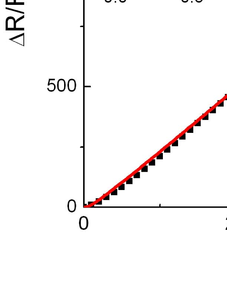
Figure 3: Normalized transverse magnetoresistance, $\Delta R/R$, as a function of magnetic field measured at T = 110 K. The solid line is a theoretical fit from 20 $\times$ 20 random resistor networks averaged over 10 realizations with $\langle\mu\rangle=0$ and $\Delta\mu^{-1}$ = 0.58 T, consistent with the PL hypothesis $\Delta\mu/\langle\mu\rangle>1$. Inset: As seen in a blow up of the low field region, the inverse of the mobility distribution width, $\Delta\mu^{-1}$, sets the approximate scale for the crossover to conventional quadratic behavior.

This functional dependence is known as Kohler’s rule, obeyed by a great number of metals and semiconductors, with a positive, quadratic MR expected to saturate for $\omega\tau\approx 1$. By contrast, in doped silver chalcogenides, the anomalous transport is characterized by a large, linear magnetoresistance that shows no sign of saturation at 60 T and extends down into the low field regime ($H\ll 1/\mu$) where one generally expects $\Delta R/R\propto H^{2}$. Moreover, the curves at different temperatures do not coincide with the scaling form $\Delta R/R=f(\omega\tau)$, but are shifted by a multiplicative factor that depends on temperature 16 .

The PL model is able to account for the linearity at low fields by showing that the linear, transverse MR of a heavily inhomogeneous semiconductor crosses over to quadratic behavior at a field set by the inverse of the mobility distribution width $\Delta\mu$, rather than the average mobility $\langle\mu\rangle$, provided that $\Delta\mu/\langle\mu\rangle>1$ . In addition, the character of the mobility distribution determines the magnitude of the linear response: at sufficiently large fields, $\Delta R/R\propto\Delta\mu H$ for strongly disordered semiconductors with $\Delta\mu/\langle\mu\rangle>1$ . Therefore, the galvanomagnetic behavior of the silver chalcogenides naturally deviates from a Kohler’s plot, since its temperature dependence is no longer simply tuned by the change in carrier mobilities, but also by the disposition of the sample inhomogeneity.

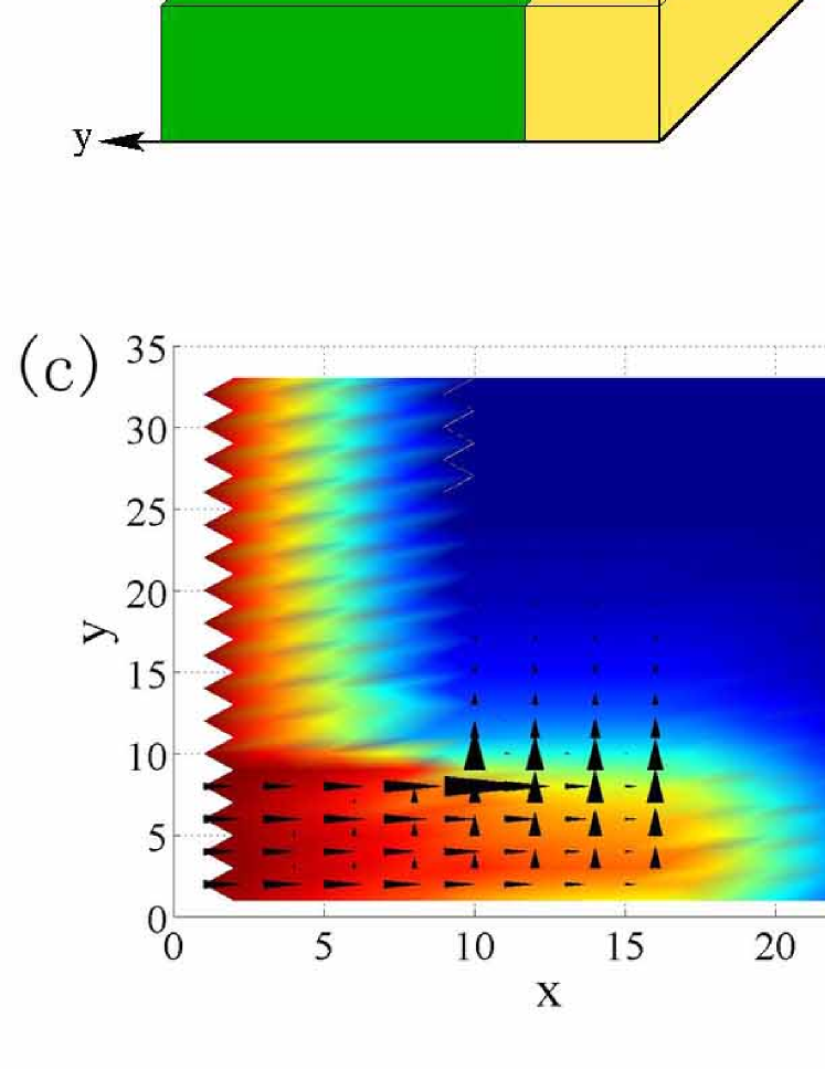
Figure 4: Visualizations of currents and voltages for the two-dimensional “percolation” pattern depicted in (a), taking $\rho_{1}/\rho_{2}$ = 10,000 and using slightly smaller networks of 12 $\times$ 16 $\times$ 24 elements for better visibility. The currents correspond to black arrows where the magnitude is given by the arrow size, while the voltages are represented by different colors, assuming the voltage drop across the sample is 1V. Panel (b) shows the currents and voltages as viewed from the top in the absence of a magnetic field, where the transport is independent of $z$. In a large magnetic field $\beta$ = 10, the current develops a component in the $z$-direction, resulting in a loss of current at the top surface as depicted in (c). Panel (d) shows a slice at $x=L_{x}/2$ that reveals the behavior of the current in the $z$-direction.

For a quantitative understanding of the temperature and field dependence of the transverse MR in silver chalcogenides, it is necessary to compare directly the theoretical predictions of the PL model with experiment. Fits to the data will yield an estimate of the mobility distribution in the silver chalcogenides and will test whether the crossover from quadratic to linear MR is set by the absolute value of the mobility $\mu$ or by the width of the mobility distribution $\Delta\mu$. We plot in Fig. 3 the transverse MR in $n$-type $\mathrm{Ag}_{2+\delta}\mathrm{Se}$ ($\delta$ = 0.0001) at both low and high fields, fit to the random resistor network model. We find that $\langle\mu\rangle=0$ yields the best fit, with $\Delta\mu^{-1}$ = 0.58$\pm$0.05 T, confirming the expectation that the silver chalcogenides are in the regime of $\Delta\mu/\langle\mu\rangle\gg 1$, with a crossover field set approximately by $\Delta\mu^{-1}$. While the value for $\Delta\mu^{-1}$ is still slightly higher than the observed crossover field, it is remarkably good given that we are considering a simple random resistor network model with only two adjustable parameters. Our toy model is oversimplified in many ways: it is two-dimensional instead of three, it is restricted to a narrow range of disorder types, and it neglects the contact effect between network disks.

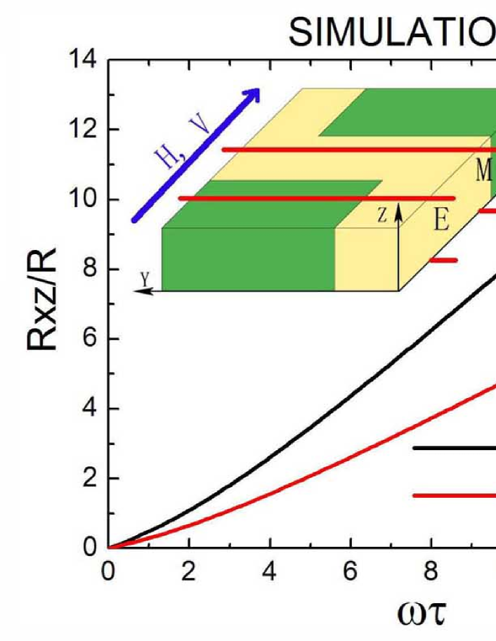
Figure 5: (a) The voltage drop measured across the thickness of $n$-type Ag₂Se, revealing distorted current flows as a direct manifestation of sample inhomogeneities (depicted in the inset). A conventional six-probe technique was used to compare signals from the edge (E) and middle (M) of the specimen. (b) Numerically simulated $R_{xz}(H)$ components of a 18 $\times$ 24 $\times$ 30 three-dimensional network (illustrated in the inset). The potential on each side of the sample was averaged over the illustrative solid lines.

Of particular interest is the fact that the electrons and holes are present in equal proportions, as indicated by $\langle\mu\rangle=0$, consistent with the claim that the magnetoresistance is most linear when both positive and negative values of the mobility can be sampled. For an inhomogeneous system, however, the averaged mobility cannot be simply obtained from a measurement of the Hall resistance. The experimental determination of the mobility distribution requires a more precise characterization of the internal structure, as a real material generally contains a small fraction of heavily doped regions imbedded into a stoichiometric background with intrinsic carrier concentration. Indeed, an unambiguous theoretical prediction for the Hall resistance has proved elusive for the random resistor network in this regime 24 .

IV.2 Current Distortions in a Longitudinal Field

The MR in conventional semiconductors is caused by the curvature of the carrier trajectories in a magnetic field. In a longitudinal geometry, where the magnetic field lies in the same direction (the $x$-direction) as the applied voltage, the carriers’ momentum in the $x$-direction is conserved for a uniform current flow, yielding a nearly negligible longitudinal MR. The diagonal tensor components $R_{xz}(H)$, representing transverse-longitudinal couplings, should be zero due to the vector nature of the magnetic field. When strong inhomogeneity exists, however, current distortions in the $y$ and $z$ directions can significantly affect the galvanomagnetic measurements.

While experiments cannot access local current patterns directly, fortunately one can numerically simulate them. Our simple two-dimensional percolation pattern in Fig. 4(a) provides an ideal starting point for demonstrating the existence of field-induced current distortions along the sample thickness. At zero field the transport is independent of $z$, due to symmetry, and there is no current in the $z$-direction (Fig. 4(b)). Once the sample is placed in a large magnetic field ($\beta\gg 1$), a substantial current flow develops in the $z$-direction. As shown in Figs. 4(c) and (d), the current enters the sample along the top surface, flows along the $z$-direction in the middle of the sample, and then exits along the bottom surface. Note that the current is parallel to the equipotentials at large fields, as expected, since the angle that the current makes with the electric field is given by $\arctan(\beta)$. The current pattern in Fig. 4(d) is reminiscent of that in a rectangular homogeneous material with perfectly conducting electrodes on the left and right boundaries [24]. There, the current distortions were induced by a mismatch of the Hall resistivity between the material and the electrodes. In this case, the mismatch is generated from the change in the angle that the current spans with the magnetic field, rather than arising from a change in the properties of the charge carriers themselves.

Experimentally, we characterize the transport in the $z$-direction of the silver chalcogenides by measuring the longitudinal-transverse coupling $R_{xz}$, i.e. the voltage drop across the sample thickness divided by the total current entering the sample. We plot in the main panel of Fig. 5(a) the $R_{xz}$ tensor component for an n-type $\mathrm{Ag_{2}Se}$ sample as a function of dimensionless field $\beta=\omega\tau$ at T = 110 K. Here, a six-probe configuration was used to compare the voltage drop at two different probe locations, and allow for later correction of possible lead misalignments ($R_{xz}(H)-R_{xz}(0)\frac{\Delta R_{zz}(H)}{R_{zz}(0)}$).

The observed finite $R_{xz}$ provides clear evidence of the predicted current distortion in the non-stoichiometric silver chalcogenides system. Moreover, except for obvious changes in the magnitude, the functional dependence on magnetic field of $R_{xz}$ appears to be rather insensitive to the location of voltage leads. Fig. 5(b) provides the calculated $R_{xz}$ components of the percolation pattern constructed from 12 $\times$ 16 $\times$ 30 elements, where the averaged potential on each side of the sample was determined by sampling along the illustrated solid lines (Fig. 5(b), inset). The simulated results show good consistency with the experimental data, as demonstrated by an increasing $R_{xz}$ with increasing H without saturation up to 14 T ($\omega\tau\sim 14$). While both experiment and simulation have a similar dependence on probe location, note that the theoretical $R_{xz}$ must decrease as we approach the boundaries because the ideal electrodes do not support a voltage drop.

The non-zero $R_{xz}$ observed in experiment and simulation indicates that the inhomogeneities are macroscopic, with a length scale that is appreciable compared to the sample dimensions. To see this, it is important to stress that the sample is not invariant with respect to a 180-degree rotation about the field axis, indicating that the current paths favor a given direction in the $y$-$z$ plane. Such symmetry breaking is not expected to occur in an isotropic system that is effectively infinite, but finite sized systems, such as our percolation pattern, can exhibit a particular chirality. However, not all the salient features of experiment are captured by our simple model. The theoretical $R_{xz}$ is purely anti-symmetric with respect to magnetic field, while the experimental $R_{xz}$ contains a substantial symmetric part. This is not surprising given that the inhomogeneities in our model are only two-dimensional. To generate a symmetric dependence of $R_{xz}$ on field, we require current flow along the $z$-direction in the absence of magnetic fields, and therefore three-dimensional inhomogeneities, so that the $z$-component of the current is not completely controlled by the field direction. Nonetheless, our simple model serves to illustrate the principle of field-induced current distortions across the sample thickness.

IV.3 Longitudinal Magnetoresistance

The longitudinal MR provides the most striking manifestation of sample inhomogeneities. As the distorted current now lies across the thickness of the sample, bending the equipotential lines (Fig. 5(a), inset), the voltage drop across the length of the sample will be reduced significantly and a negative MR can emerge. We plot in Fig. 6 the normalized longitudinal MR of $n$-type $\mathrm{Ag_{2}Te}$ as a function of temperature and sample thickness, and see a pronounced negative MR in the bulk sample (400 $\mu$m) for T $>$ 50 K. The maximum in the negative MR at T = 110 K corresponds to the crossover from intrinsic to extrinsic semiconducting behavior, where the distortions of current become the strongest as the fluctuations in mobility can veer from positive to negative. However, this effect is diminished for thinner samples, such that there is no negative MR observed up to $H$ = 14 T for thickness 20 $\mu$m. This demonstrates not only that current flow across the sample thickness is crucial for the appearance of negative MR, but that the critical thickness of 20 $\mu$m gives a measure of the inhomogeneity length scale. The effects of spatial randomness are suppressed completely if the size of the system becomes comparable to the characteristic inhomogeneity length scale in one dimension.

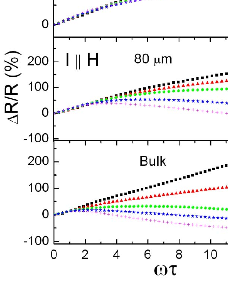
Figure 6: Normalized longitudinal magnetoresistance vs. sample thickness of $n$-type Ag₂Te. The negative component of the magnetoresistance diminishes in thinner crystals, and the inhomogeneity length scale is determined by the thickness where the negative MR eventually disappears (20 $\mu$m).

We now compare the experimental results to simulations. For the two-dimensional percolation pattern in Fig. 7(a) with $\rho_{1}/\rho_{2}$ = 10,000, we know from Fig. 4(c) that there is a flow of current away from the surface at high magnetic fields. Hence a negative MR would be obtained from a four-probe measurement where the voltage drop is measured by placing probes on the top surface of the sample. However, the induced current distortions also increase the actual resistance of the sample, and we find that this effect dominates, resulting in the same positive linear magnetoresistance as would be obtained from a two-probe measurement (Fig. 7(b)). This is consistent with the experiments, where the magnetoresistance becomes both positive and quasi-linear when we reduce the inhomogeneities in the $z$-direction by thinning the sample. Similar to the case of transverse MR, the linearity of the longitudinal MR is derived from the Hall resistance contributed by distorted current paths, namely by the currents in the $z$-direction of Fig. 4(d). The magnitude of the longitudinal MR, however, is reduced when we decrease $\rho_{1}/\rho_{2}$, as the magnetoresistance always saturates at a field scale set by $\rho_{1}/\rho_{2}$. As expected, when we take the limit $L_{z}\rightarrow 0$ in Fig. 2(d), we find that $\Delta R/R\propto L_{z}$, so that there is no magnetoresistance in a truly two-dimensional system.

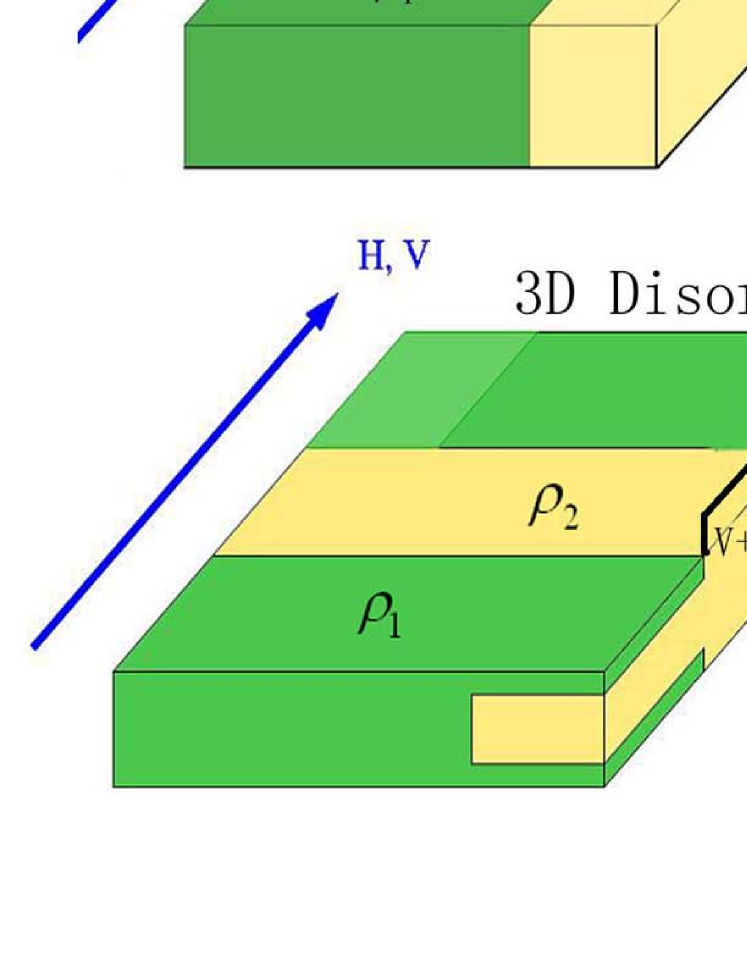
Figure 7: Longitudinal magnetoresistance simulated using 18 $\times$ 24 $\times$ 24 elements for the two-dimensional pattern and 18 $\times$ 24 $\times$ 40 elements for three-dimensional pattern. At a sufficiently large resistivity ratio, corresponding to true three-dimensional behavior, a negative longitudinal MR emerges.

In order to obtain a negative magnetoresistance, one requires the current to be depleted from the surface faster than the increase in resistance. Since experiments imply that this scenario is possible when there are inhomogeneities along the $z$-direction, we consider a slight modification of our toy model to include three-dimensional disorder, as depicted in Fig. 7(c). We perform a four-probe measurement by averaging voltages along the solid lines in the $y$-direction, and then take the component of the voltage difference that is symmetric with respect to the magnetic field. Referring to Fig. 7(d), we find a substantial negative magnetoresistance when $\rho_{1}/\rho_{2}$ = 10,000, confirming that three-dimensional inhomogeneities are responsible for the negative longitudinal MR observed in the silver chalcogenides. It is of interest to note that there is always an upturn in the negative magnetoresistance at high fields for the simple models we considered, but it is unclear whether this is generic for the infinite system.

V Conclusions

In this paper, we have compared directly the galvanomagnetic transport experiments on $\mathrm{Ag}_{2\pm\delta}\mathrm{Se}$ and $\mathrm{Ag}_{2\pm\delta}\mathrm{Te}$ with theoretical simulations of inhomogeneous conductors in both two and three dimensions. By fitting the linear transverse MR with the PL 2D random resistor network model, we have demonstrated that the silver chalcogenides contain roughly equal proportions of electron- and hole-like regions, and that the field scale for the onset of linearity is set by the width of the mobility distribution rather than the average mobility. Extending the model to three dimensions, we find that simple realizations of macroscopic disorder are able to reproduce the observed finite longitudinal-transverse coupling $R_{xz}$ and the negative longitudinal MR in the silver chalcogenides. Moreover, visualizations of the current distortions across the thickness dimension illustrate the depletion of current at the sample surface that is crucial for the phenomenon. Future work is required to extend the theoretical results to the infinite system and to characterize precisely the types of disorder which give rise to the biggest magnetoresistive response.

- (1) M. B. Isichenko, Rev. Mod. Phys. 64, 961 (1992).
- (2) C. Herring, J. Appl. Phys. 31, 1939 (1960).
- (3) Y. A. Dreizin and A. M. Dykhne, Sov. Phys. JETP 36, 127 (1973).
- (4) B. Y. Balagurov, Sov. Phys. Solid State 28, 1694 (1986).
- (5) D. Stroud and F. P. Pan, Phys. Rev. B 13, 1434 (1976).
- (6) D. J. Bergman and D. G. Stroud, Phys. Rev. B 62, 6603 (2000).
- (7) A. M. Dykhne, Sov. Phys. JETP 32, 348 (1971).
- (8) B. Y. Balagurov, Sov. Phys. Solid State 20, 1922 (1978).
- (9) T. Thio and S. A. Solin, Appl. Phys. Lett. 72, 3497 (1998).
- (10) T. Thio, S. A. Solin, J. W. Bennett, D. R. Hines, M. Kawano, N. Oda, and M. Sano, Phys. Rev. B 57, 12239 (1998).
- (11) P. Junod, Helv. Phys. Acta 32, 567 (1959).
- (12) R. Xu, A. Husmann, T.F. Rosenbaum, M.-L. Saboungi, J.E. Enderby, and P. B. Littlewood, Nature 390, 57 (1997).
- (13) I.S. Chuprakov and K.H. Dahmen, Appl. Phys. Lett. 72, 2165 (1998).
- (14) Z. Ogorelec, A. Hamzic and M. Basletic, Europhys. Lett. 46, 56 (1999).
- (15) H. S. Schnyders, M.-L. Saboungi and T. F. Rosenbaum, Appl. Phys. Lett. 76, 1717 (2000).
- (16) A. Husmann, J. B. Betts, G. S. Boebinger, A. Migliori, T. F. Rosenbaum, and M.-L. Saboungi, Nature 417, 421 (2002).
- (17) M. Lee, T. F. Rosenbaum, M.-L. Saboungi, and H. S. Schnyders, Phys. Rev. Lett. 88, 066602 (2002).
- (18) A. A. Abrikosov, Phys. Rev. B 58, 2788 (1998).
- (19) M. M. Parish and P. B. Littlewood, Nature 426, 162 (2003).
- (20) Y. Kumashiro, T. Ohachi and I. Taniguchi, Solid State Ionics 86-88, 761 (1996).
- (21) A. A. Abrikosov, Europhys. Lett. 49, 789 (2000).
- (22) F. Y. Yang, Kai Liu, Kimin Hong, D. H. Reich, P. C. Searson and C. L. Chien, Science 284, 1335 (1999).
- (23) Jingshi Hu and T. F. Rosenbaum, to be published.
- (24) M. M. Parish and P. B. Littlewood, Phys. Rev. B 72, 094417 (2005).
- (25) V. Guttal and D. Stroud, Phys. Rev. B 71, 201304(R) (2005).
- (26) R. Magier and D. J. Bergman, Phys. Rev. B 74, 094423 (2006).
- (27) V. Guttal and D. Stroud, Phys. Rev. B 73, 085202 (2006).
- (28) Jingshi Hu, T. F. Rosenbaum and J. B. Betts, Phys. Rev. Lett. 95, 186603 (2005).
- (29) A. B. Pippard, Magnetoresistance in Metals (Cambridge University Press, Cambridge, 1989).
- (30) S. Bulgadaev, Phys. Lett. A 344, 280 (2005).
- (31) M. B. Isichenko and Y. L. Kalda, Sov. Phys. JETP 72, 126 (1991).
- (32) M. B. Isichenko and J. Kalda, J. Moscow Phys. Soc. 2, 55 (1992).
- (33) A. K. Sarychev, D. J. Bergman, and Y. M. Strelniker, Phys. Rev. B 48, 3145 (1993).