Magneto-elastic waves in crystals of magnetic molecules

Abstract

We study magneto-elastic effects in crystals of magnetic molecules. Coupled equations of motion for spins and sound are derived and the possibility of strong resonant magneto-acoustic coupling is demonstrated. Dispersion laws for interacting linear sound and spin excitations are obtained for bulk and surface acoustic waves. We show that ultrasound can generate inverse population of spin levels. Alternatively, the decay of the inverse population of spin levels can generate ultrasound. Possibility of solitary waves of the magnetization accompanied by the elastic twists is demonstrated.

I Introduction

Crystals of molecular magnets are paramagnets book ; dipolar that have the ability to maintain macroscopic magnetization for a long time in the absence of the external magnetic field. This is a consequence of the magnetic bi-stability of individual molecules Sessoli that in many respects behave as superparamagnetic particles. The latter is due to a large spin (e.g., $S=10$ for Mn-12 and Fe-8) and high magnetic anisotropy of the molecules. Together with quantization of spin energy levels this leads to a distinctive feature of molecular magnets: A staircase hysteresis curve in a macroscopic measurement of the magnetization. Friedman

Hybridization of electron paramagnetic resonance (EPR) with longitudinal ultrasonic waves has been studied by Jacobsen and Stevens JS within a phenomenological model of magneto-elastic interaction proportional to the magnetic field. General theory of magneto-elastic effects on the phonon dispersion and the sound velocity in conventional paramagnets has been developed by Dohm and Fulde. DF The advantage of molecular magnets is that they, unlike conventional paramagnets, can be prepared in a variety of magnetic states even in the absence of the magnetic field. Spontaneous transitions between spin levels in molecular magnets are normally due to the emission and absorption of phonons. Interactions of molecular spins with phonons have been studied in the context of magnetic relaxation, Villain ; GC-97 ; Loss ; Comment conservation of angular momentum, EC-94 ; EC-Martinez ; CGS phonon Raman processes, Raman and phonon superradiance. SR Parametric excitation of acoustic modes in molecular magnets has been studied. Tokman ; Xie It has been suggested that surface acoustic waves can produce Rabi oscillations of magnetization in crystals of molecular magnets. Rabi In this paper we study coupled dynamics of paramagnetic spins and elastic deformations at a macroscopic level.

When considering magneto-elastic waves in paramagnets the natural question is why the adjacent spins should rotate in unison rather than behave independently. In ferromagnets the local alignment of spins is due to the strong exchange interaction. Due to this interaction the length of the local magnetization is a constant throughout the ferromagnet. We shall argue now that a somewhat similar quantum effect exists in a system of weakly interacting two-level entities described by a fictitious spin $1/2$. Indeed, since any product of Pauli matrices reduces to a single Pauli matrix ${\sigma}_{\alpha}$, interaction of $N$ independent two-state systems with an arbitrary field ${\bf A}({\bf r})$ should be linear on ${\sigma}_{\alpha}$,

$${\cal{H}}=\sum_{n=1}^{N}g_{\alpha\beta}\sigma_{\alpha}^{(n)}A_{\beta}({\bf r}_{n})\;,$$ (1)

where ${\bm{\sigma}}^{(n)}$ describes a two-state system located at a point ${\bf r}={\bf r}_{n}$. If ${\bf A}$ was independent of coordinates, then the Hamiltonian (1) would reduce to

$${\cal{H}}=g_{\alpha\beta}\Sigma_{\alpha}A_{\beta}\;,$$ (2)

where

$${\bf\Sigma}=\sum_{n=1}^{N}{\bm{\sigma}}^{(n)}$$ (3)

is the total fictitious spin of the system. In this case the interaction Hamiltonian would commute with ${\bf\Sigma}^{2}$, thus preserving the length of the total fictitious “magnetization”. This observation is crucial for understanding Dicke superradiance: Dicke A system of independent two-state entities behaves collectively in a field whose wavelength significantly exceeds the size of the system. When the wavelength of the field is small compared to the size of the system but large compared to the distance between the two-state entities, the same argument can be made about the rigidity of ${\bf\Sigma}=\sum{\bm{\sigma}}^{(n)}$ summed up over the distances that are small compared to the wavelength. Consequently, the system that has been initially prepared in a state with all spins up, and then is allowed to evolve through interaction with a long-wave Bose field, should conserve the length of the local “magnetization” in the same way as ferromagnets do.

The relevance of the above argument to the dynamics of magnetic molecules interacting with elastic deformations becomes obvious when only two spin levels are important. This is the case when the low-energy dynamics of the molecular magnet is dominated by, e.g., tunnel split spin-levels or when the magneto-acoustic wave is generated by a pulse of sound of resonant frequency. Recently, experiments with surface acoustic waves in the GHz range have been performed in crystals of molecular magnets. Alberto1 The existing techniques, in principle, allow generation of acoustic frequencies up to 100 GHz. Santos This opens the possibility of resonant interaction of generated ultrasound with spin excitations. In this paper we study coupled magneto-elastic waves in the ground state of a crystal of molecular magnets. We derive equations describing macroscopic dynamics of sound and magnetization and show that high-frequency ultrasound interacts strongly with molecular spins when the frequency of the sound equals the distance between spin levels. We obtain the dispersion relation for magneto-elastic waves and show that non-linear equations of motion also possess solutions describing solitary waves of magnetization coupled to the elastic twists.

The paper is organized as follows. The model of spin-phonon coupling is discussed in Section II where coupled magneto-elastic equation are derived. Linear magneto-elastic waves are studied in Section III where we obtain dispersion laws for bulk and surface acoustic waves. Non-linear solitary waves are studied in Section IV. Suggestions for experiments are made in Section V.

II Model of magneto-elastic coupling

We consider a molecular magnet interacting with a local crystal field described by a phenomenological anisotropy Hamiltonian $\hat{\mathcal{H}}_{A}$. The spin cluster is assumed to be more rigid than its elastic environment, so that the long-wave crystal deformations can only rotate it as a whole but cannot change its inner structure responsible for the parameters of the Hamiltonian $\hat{\cal{H}}_{A}$. This approximation should apply to many molecular magnets as they typically have a compact magnetic core inside a large unit cell of the crystal. In the presence of deformations of the crystal lattice, given by the displacement field ${\bf u}({\bf r})$, local anisotropy axes defined by the crystal field are rotated by the angle

$$\delta{\bm{\phi}}({\bf r},t)=\frac{1}{2}\nabla\times{\bf u}({\bf r},t)\,.$$ (4)

As a consequence of the full rotational invariance of the system (spins + crystal lattice), the rotation of the lattice is equivalent to the rotation of the operator $\hat{\bf S}$ in the opposite direction, which can be performed by the $(2S+1)\times(2S+1)$ matrix in the spin space, CGS

$$\hat{\bf S}\rightarrow\hat{R}^{-1}\hat{\bf S}\hat{R},\qquad\hat{R}=e^{i\hat{\bf S}\cdot\delta{\bm{\phi}}}\,.$$ (5)

Therefore, the total Hamiltonian of a molecular magnet in the magnetic field ${\bf B}$ must be written as

$$\hat{\mathcal{{H}}}=e^{-i\hat{\bf S}\cdot\delta{\bm{\phi}}}\,\hat{\mathcal{{H}}}_{A}\,e^{i\hat{\bf S}\cdot\delta{\bm{\phi}}}+\hat{\mathcal{H}}_{Z}+\hat{\mathcal{H}}_{ph}\,,$$ (6)

where $\hat{\mathcal{H}}_{A}$ is the anisotropy Hamiltonian in the absence of phonons, $\hat{\mathcal{H}}_{Z}=-g\mu_{B}{\bf B}\cdot\hat{{\bf S}}$ is the Zeeman Hamiltonian and $\hat{\mathcal{H}}_{ph}$ is the Hamiltonian of harmonic phonons. The angle of rotation produced by the deformation of the lattice is small, so one can expand Hamiltonian (6) to first order in the angle $\delta\phi$ and obtain

$$\hat{\mathcal{H}}\simeq\hat{\mathcal{H}}_{0}+\hat{\mathcal{H}}_{s-ph}\,,$$ (7)

where $\hat{\mathcal{H}}_{0}$ is the Hamiltonian of non-interacting spins and phonons

$$\hat{\mathcal{H}}_{0}=\hat{\mathcal{H}}_{S}+\hat{\mathcal{H}}_{ph}\,,\qquad\hat{\mathcal{H}}_{S}=\hat{\mathcal{H}}_{A}+\hat{\mathcal{H}}_{Z}\,,$$ (8)

and $\hat{\mathcal{H}}_{s-ph}$ is the spin-phonon interaction term, given by

$$\hat{\mathcal{H}}_{s-ph}=i\left[\hat{\mathcal{H}}_{A},\hat{{\bf S}}\right]\cdot\delta{\bm{\phi}}\,.$$ (9)

II.1 Coupling of spins to the elastic twists

For certainty, we consider a crystal of molecular magnets with the anisotropy Hamiltonian

$$\hat{\cal{H}}_{A}=-D\hat{S}_{z}^{2}+\hat{V}\,,$$ (10)

where $\hat{V}$ is a small term that does not commute with the $\hat{S}_{z}$ operator. This term is responsible for the tunnel splitting, $\Delta$, of the levels on resonance.

At low temperature and small magnetic field, $k_{B}T,g\mu_{B}B\lesssim\Delta$, when the frequency of the displacement field ${\bf u}({\bf r})$ satisfies $\omega\ll 2DS/\hbar$, only the two lowest states of $\hat{\mathcal{H}}_{A}$ are involved in the evolution of the system. Thus, one can reduce the spin-Hamiltonian of the molecular magnet to an effective two-state Hamiltonian in terms of pseudospin-$1/2$ operators $\hat{\bf\sigma}_{i}$,

$$\hat{\mathcal{H}}_{S}^{(eff)}=-\frac{1}{2}\,(W{\bf e}_{z}+\Delta{\bf e}_{x})\cdot\hat{\bm{\sigma}}\,,$$ (11)

where $\hat{\sigma}_{i}$ are the Pauli matrices in the basis of the $\hat{S}_{z}$-states close to the resonance between $|S\rangle$ and $|-S\rangle$, and $W=E_{S}-E_{-S}$ is the energy difference for the resonant states at $\Delta=0$. The non-degenerate eigenfunctions of $\hat{\mathcal{H}}_{S}^{(eff)}$ are

$$|\psi_{\mp}\rangle=\frac{1}{\sqrt{2}}\left(C_{\pm}|S\rangle\mp C_{\mp}|-S\rangle\right)$$ (12)

with

$$C_{\pm}=\sqrt{1\pm\frac{W}{\sqrt{\Delta^{2}+W^{2}}}}\,.$$ (13)

In terms of $|\psi_{\mp}\rangle$ the Hamiltonian (11) can be written as

$$\hat{\mathcal{H}}_{S}^{(eff)}=-\frac{1}{2}\,\sqrt{W^{2}+\Delta^{2}}\,\hat{\tilde{\sigma}}_{z}\,,$$ (14)

where $\hat{\tilde{\sigma}}_{i}$ are now the Pauli matrices in the new basis $|\psi_{\pm}\rangle$, i.e., $\hat{\tilde{\sigma}}_{z}=|\psi_{+}\rangle\langle\psi_{+}|-|\psi_{-}\rangle\langle\psi_{-}|$. The projection of the spin-phonon interaction Hamiltonian (9) onto this new two-state basis results in

$$\hat{\mathcal{H}}_{s-ph}^{(eff)}=\sum_{i,j=\pm}\langle\psi_{i}|\hat{\mathcal{H}}_{s-ph}|\psi_{j}\rangle|\psi_{i}\rangle\langle\psi_{j}|=\delta\phi_{z}S\Delta\hat{\tilde{\sigma}}_{y}\,,$$ (15)

with $\hat{\tilde{\sigma}}_{y}=-i|\psi_{+}\rangle\langle\psi_{-}|+i|\psi_{-}\rangle\langle\psi_{+}|$. The total Hamiltonian (6) of a single molecular magnet becomes

$$\hat{\mathcal{H}}^{(eff)} = -\frac{1}{2}\,{\bf b}^{(eff)}\cdot\hat{\tilde{\bm{\sigma}}}+\hat{\mathcal{H}}_{ph}\,,$$

$${\bf b}^{(eff)} = \sqrt{W^{2}+\Delta^{2}}\,{\bf e}_{z}-2\delta\phi_{z}S\Delta\,{\bf e}_{y}\,.$$ (16)

Here we have assumed that the perturbation introduced by the spin-phonon interaction is much smaller than the perturbation $\hat{V}$ producing the splitting $\Delta$, which will usually be the case. Note also that $\Delta$ and $W$ can in general be made ${\bf r}$-dependent to account for possible inhomogeneities of the crystal.

When considering magneto-elastic excitations we will need to know whether they are accompanied by a non-zero local magnetization of the crystal. For that reason it is important to have the magnetic moment of the molecule,

$$m_{z}=g\mu_{B}\langle S_{z}\rangle\,,$$ (17)

(with $g$ being the gyromagnetic ratio and $\mu_{B}$ being the Bohr magneton), in terms of its wave function

$$|\Psi\rangle=K_{+}|\psi_{+}\rangle+K_{-}|\psi_{-}\rangle\,,$$ (18)

where $K_{\pm}$ are arbitrary complex numbers satisfying $|K_{-}|^{2}+|K_{+}|^{2}=1$. With the help of Eq. (12) one obtains

$$\frac{\langle S_{z}\rangle}{S} = \frac{W}{\sqrt{W^{2}+\Delta^{2}}}\left(|K_{-}|^{2}-|K_{+}|^{2}\right)$$ (19)

$$+ \frac{\Delta}{\sqrt{W^{2}+\Delta^{2}}}\left(K_{+}^{*}K_{-}+K_{+}K_{-}^{*}\right)$$

$$= \frac{\Delta\langle\hat{\tilde{\sigma}}_{x}\rangle-W\langle\hat{\tilde{\sigma}}_{z}\rangle}{\sqrt{W^{2}+\Delta^{2}}}\,.$$

II.2 Magneto-elastic equations

We want to describe our system of $N$ spins in terms of the spin field

$$\hat{\bf n}({\bf r})=\sum_{i}^{N}\hat{\tilde{\bm{\sigma}}}_{i}\delta({\bf r}-{\bf r}_{i})\,,$$ (20)

satisfying commutation relations

$$\left[\hat{n}_{\alpha}({\bf r}),\hat{n}_{\beta}({\bf r}^{\prime})\right]=2i\epsilon_{\alpha\beta\gamma}\hat{n}_{\gamma}({\bf r})\delta({\bf r}-{\bf r}^{\prime})\,.$$ (21)

In terms of this field the total Hamiltonian becomes

$$\hat{\mathcal{H}}=-\frac{1}{2}\int d^{3}r\,\hat{\bf n}({\bf r})\cdot{\bf b}^{(eff)}({\bf r})+\hat{\mathcal{H}}_{ph}\,.$$ (22)

The classical pseudo-spin field ${\bf n}({\bf r},t)$ can be defined as

$${\bf n}({\bf r},t)=\langle\hat{\bf n}({\bf r})\rangle\,,$$ (23)

where $\langle...\rangle$ contains the average over quantum spin states and the statistical average over spins inside a small volume around the point ${\bf r}$. If the size of that volume is small compared to the wavelength of the phonon displacement field, then, as has been discussed in the Introduction, ${\bf n}^{2}({\bf r})$ should be approximately constant in time. According to equations (17), (19) and (20), the magnetization is given by

$$M_{z}({\bf r})=g\mu_{B}S\;\frac{\Delta\,n_{x}({\bf r})-W\,n_{z}({\bf r})}{\sqrt{W^{2}+\Delta^{2}}}\,.$$ (24)

The dynamical equation for the classical pseudo-spin field ${\bf n}({\bf r},t)$ is

$$i\hbar\frac{\partial{\bf n}({\bf r},t)}{\partial t}=\left\langle[\hat{\mathcal{H}},\hat{\bf n}]\right\rangle\,,$$ (25)

which, with the help of Eq. (21), can be written as

$$\hbar\frac{\partial{\bf n}({\bf r},t)}{\partial t}={\bf n}({\bf r},t)\times{\bf b}^{(eff)}({\bf r},t)\,.$$ (26)

In this treatment we are making a common assumption that averaging over spin and phonon states can be done independently. This approximation is expected to be good in the long-wave limit.

The dynamical equation for the displacement field is

$$\rho\frac{\partial^{2}u_{\alpha}}{\partial t^{2}}=\sum_{\beta}\frac{\partial\sigma_{\alpha\beta}}{\partial x_{\beta}}\,,$$ (27)

where $\sigma_{\alpha\beta}={\partial h}/\partial e_{\alpha\beta}$ is the stress tensor, $e_{\alpha\beta}=\partial u_{\alpha}/\partial x_{\beta}$ is the strain tensor, $h$ is the Hamiltonian density of the system in $\hat{\mathcal{H}}=\int d^{3}r\,h({\bf r})$, and $\rho$ is the mass density. Note that the stress tensor has an antisymmetric part originating from the magneto-elastic interaction in the Hamiltonian,

$$\sigma_{\alpha\beta} = \sigma_{\alpha\beta}^{(s)}+\sigma_{\alpha\beta}^{(a)}\,,$$

$$\sigma_{\alpha\beta}^{(a)} = \frac{1}{2}S\Delta\,n_{y}({\bf r})\epsilon_{z\alpha\beta}\,.$$ (28)

This implies that at each point ${\bf r}$ there is a torque per unit volume,

$$\tau_{\alpha}({\bf r})=-\delta_{\alpha z}S\Delta\,n_{y}({\bf r})\,,$$ (29)

created by the interaction with the magnetic system. This effect can be viewed as the local Einstein – de Haas effect: Spin rotation produces a torque in the crystal lattice due to the necessity to conserve angular momentum. With the help of equations (II.1), (22), and (27), using standard results of the theory of elasticity, one obtains

$$\frac{\partial^{2}{u}_{\alpha}}{\partial t^{2}}-c_{t}^{2}{\bm{\nabla}}^{2}{u}_{\alpha}-(c_{l}^{2}-c_{t}^{2}){\nabla}_{\alpha}({\bm{\nabla}}\cdot{\bf u})=\frac{S\Delta}{2\rho}\,\epsilon_{z\alpha\beta}{\nabla}_{\beta}n_{y}\,,$$ (30)

where $c_{l}$ and $c_{t}$ are velocities of longitudinal and transverse sound. The source of deformation in the right hand side of this equation is due to the above-mentioned torque generated by the spin rotation.

Equations (26) and (30) describe coupled motion of the pseudospin field ${\bf n}({\bf r},t)$ and the displacement field ${\bf u}({\bf r},t)$. It is easy to see from these equations that in accordance with the argument presented in the Introduction $n_{x}^{2}+n_{y}^{2}+n_{z}^{2}$ is independent of time. It may, nevertheless, depend on coordinates, reflecting the structure of the initial state. In this paper we study cases in which the crystal of molecular magnets was initially prepared in the ground state ${\bf n}=n_{0}{\bf e}_{z}$ with $n_{0}$ being the concentration of magnetic molecules. In this case the dynamics of ${\bf n}({\bf r})$ described by equations (26) and (30) reduces to its rotation, with the length of ${\bf n}({\bf r})$ being a constant $n_{0}$. Remarkably, this situation is similar to a ferromagnet, despite the absence of the exchange interaction.

III Linear magneto-elastic waves

III.1 Bulk waves

For magnetic molecules whose magnetic cores are more rigid than their environments, only the transverse part of the displacement field (with $\nabla\cdot{\bf u}({\bf r})=0$) interacts with the magnetic degrees of freedom. This is a consequence of the fact that the elastic deformation produced by the rotation of local magnetization is a local twist of the crystal lattice, required by the conservation of angular momentum. Let us consider then a transverse plane wave propagating along the X-axis. From Eqs. (26) and (30) one obtains

$$\frac{\partial^{2}u_{y}}{\partial t^{2}}-c_{t}^{2}\frac{\partial^{2}u_{y}}{\partial x^{2}}=-\frac{S\Delta}{2\rho}\frac{\partial n_{y}}{\partial x}$$

$$\hbar\frac{\partial n_{x}}{\partial t}=n_{y}\sqrt{W^{2}+\Delta^{2}}-n_{z}S\Delta\frac{\partial u_{y}}{\partial x}$$

$$\hbar\frac{\partial n_{y}}{\partial t}=-n_{x}\sqrt{W^{2}+\Delta^{2}}$$

$$\hbar\frac{\partial n_{z}}{\partial t}=S\Delta n_{x}\frac{\partial u_{y}}{\partial x}\;.$$ (31)

We shall study linear waves around the ground state $|\psi_{+}\rangle$ corresponding to $n_{z}=n_{0},n_{x,y}=0,u_{y}=0$. The perturbation around this state results in nonzero $n_{x,y}$ and $u_{y}$. Linearized equations of motion are

$$\frac{\partial^{2}u_{y}}{\partial t^{2}}-c_{t}^{2}\frac{\partial^{2}u_{y}}{\partial x^{2}}=-\frac{S\Delta}{2\rho}\frac{\partial n_{y}}{\partial x}$$

$$\hbar\frac{\partial n_{x}}{\partial t}=n_{y}\sqrt{W^{2}+\Delta^{2}}-S\Delta n_{0}\frac{\partial u_{y}}{\partial x}$$

$$\hbar\frac{\partial n_{y}}{\partial t}=-n_{x}\sqrt{W^{2}+\Delta^{2}}\;.$$ (32)

For $u_{y},n_{x,y}\propto\exp(iqx-i\omega t)$, the above equations become

$$(\omega^{2}-c_{t}^{2}q^{2})u_{y}-iq\frac{S\Delta}{2\rho}n_{y}=0$$

$$iq\frac{n_{0}S\Delta\sqrt{W^{2}+\Delta^{2}}}{\hbar^{2}}u_{y}+\left(\omega^{2}-\frac{W^{2}+\Delta^{2}}{\hbar^{2}}\right)n_{y}=0\,.$$

\begin{picture}(20.0,5.0)\centerline{\hbox{\psfig{width=227.62204pt}}} \end{picture}

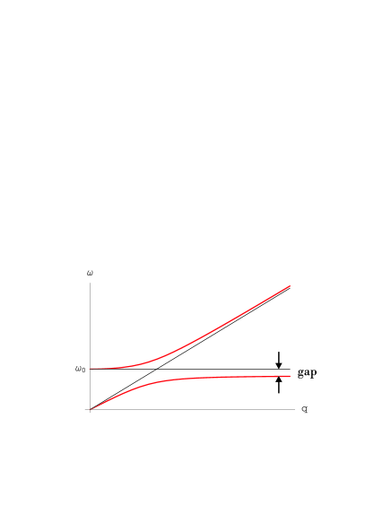
Figure 1: Interacting sound and spin modes. Notice the gap below spin resonance $\omega_{0}$.

The spectrum of coupled excitations is given by

$$(\omega^{2}-c_{t}^{2}q^{2})\left(\omega^{2}-\frac{W^{2}+\Delta^{2}}{\hbar^{2}}\right)=\frac{n_{0}S^{2}\Delta^{2}\sqrt{W^{2}+\Delta^{2}}}{2\rho\hbar^{2}}q^{2}\;.$$ (34)

In the vicinity of the resonance,

$$c_{t}q_{0}=\frac{\sqrt{W^{2}+\Delta^{2}}}{\hbar}\equiv\omega_{0}\;,$$ (35)

one can write

$$\omega=\omega_{0}(1+\delta)\;$$ (36)

with $\delta$ to be determined by the dispersion relation. Substituting equations (35) and (36) into Eq. (34), one obtains

$$\delta=\pm\sqrt{\frac{n_{0}S^{2}\Delta^{2}}{8\rho c_{t}^{2}\hbar\omega_{0}}}\;,$$ (37)

that describes the splitting of two coupled modes at the resonance. The repulsion of elastic and spin modes is illustrated in Fig. 1. The relative splitting of the modes reaches maximum at $W=0$ ($\hbar\omega_{0}=\Delta$):

$$2|\delta_{max}|=\sqrt{\frac{n_{0}S^{2}\Delta}{2\rho c_{t}^{2}}}=S\sqrt{\frac{\Delta}{2{\rm M}c_{t}^{2}}}\;,$$ (38)

where ${\rm M}=\rho/n_{0}$ is the mass of the volume containing one molecule of spin $S$. Notice also another consequence of Eq. (34): The presence of the energy gap below $\omega_{0}=\sqrt{W^{2}+\Delta^{2}}/\hbar$ (see Fig. 1). The value of the gap follows from Eq. (34) at large $q$. It equals $2\delta^{2}\omega_{0}$. This effect is qualitatively similar to the one obtained in Ref. JS, from an ad hoc model of spin-phonon interaction. In contrast with that model our results for the splitting of the modes and for the gap do not contain any unknown interaction constants as they are uniquely determined by the conservation of the total angular momentum (spin + crystal lattice).

According to equations (III.1) and (34) the Fourier transforms of $n_{y}$ and $u_{y}$ are related through

$$\frac{n_{y}}{n_{0}}=iS\frac{\omega_{0}^{2}}{\omega_{0}^{2}-\omega^{2}}\;\frac{\Delta}{\hbar\omega_{0}}\;qu_{y}\,.$$ (39)

Due to the condition of the elastic theory $qu_{y}\ll 1$, the absolute value of the ratio $n_{y}/n_{0}$ is generally small, unless $\omega$ is close to $\omega_{0}$. This means that away from the resonance the sound cannot significantly change the population of excited spin states. At the magneto-elastic resonance, substituting equations (36) and (37) into the above equation, one obtains:

$$\frac{|n_{y}|_{res}}{n_{0}}=\left(\frac{2{\rm M}\omega_{0}}{\hbar}\right)^{1/2}|u_{y}|\,.$$ (40)

Although this relation is valid only at $|n_{y}|\ll n_{0}$, it allows one to estimate the amplitude of ultrasound that will significantly affect populations of spin states. We shall postpone the discussion of this effect until Section V. Meantime let us compute the magnetization generated by the linear elastic wave, $u_{y}=u_{0}\cos[q_{0}(x-c_{t}t)])$, in resonance with our two-state spin system. The last of Eqs. (III.1) yields $n_{x}=i(\omega/\omega_{0})n_{y}$. Then, with the help of Eq. (24) and Eq. (40) one obtains

$$M_{z}=g\mu_{B}S\frac{\Delta}{\hbar\omega_{0}}\left(\frac{2{\rm M}c_{t}^{2}}{\hbar\omega_{0}}\right)^{1/2}q_{0}u_{0}\cos[q_{0}(x-c_{t}t)]\,.$$ (41)

So far we have investigated coupled magneto-elastic waves in the vicinity of the ground state, $n_{z}=n_{0}$. Eqs. (III.1) also allow one to obtain the increment, $\Gamma$, of the decay of the unstable macroscopic state of the crystal, $n_{z}=-n_{0}$, in which all molecules are initially in the excited state $|\psi_{-}\rangle$. In fact, the result can be immediately obtained from equations (III.1) – (34) by replacing $n_{0}$ with $-n_{0}$. It is then easy to see from Eq. (34) that in the vicinity of the resonance the frequency acquires an imaginary part that attains maximum at the resonance where

$$\omega=\omega_{0}(1\pm i|\delta|)\,.$$ (42)

The mode growing at the rate $\Gamma=\omega_{0}|\delta|$ represents the decay of $|\psi_{-}\rangle$ spin states into $|\psi_{+}\rangle$ spin states, separated by energy $\hbar\omega_{0}$. This decay is accompanied by the exponential growth of the amplitude of ultrasound of frequency $\omega_{0}$.

III.2 Surface waves

Magneto-elastic coupling in crystals of molecular magnets can be studied with the help of surface acoustic waves (see Discussion). To describe the surface waves we chose a geometry in which the surface of interest is the $XZ$-plane and the solid extends to $y>0$ with waves running along the direction that makes an angle $\theta$ with the $X$-axis, see Fig. 2.

\begin{picture}(15.0,3.0)\centerline{\hbox{\psfig{width=199.16928pt}}} \end{picture}

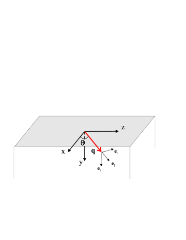
Figure 2: Geometry of the problem with surface acoustic waves.

As usual LL we assume that the displacement field ${\bf u}({\bf r},t)$ and the components $n_{x}({\bf r},t),n_{y}({\bf r},t)$ have the form

$$A=A_{0}e^{-\alpha y}e^{i(q_{x}x+q_{z}z)}e^{-i\omega t}\,.$$ (43)

It is convenient to express the components of the displacement field in the coordinate system defined by $({\bf e}_{l},{\bf e}_{t},{\bf e}_{p})$, see Fig. 2,

$$u_{x} = u_{l}\cos\theta-u_{t}\sin\theta$$

$$u_{y} = u_{p}$$

$$u_{z} = u_{l}\sin\theta+u_{t}\cos\theta\,.$$ (44)

Equations of motion for $u_{l}$, $u_{t}$, and $u_{p}$ follow from Eq. (30):

$$\left[\omega^{2}+c_{t}^{2}(\alpha^{2}-q^{2})\right]u_{t} + \frac{S}{2\rho}\,\alpha\Delta\sin\theta n_{y}=0$$

$$\left[\omega^{2}+c_{t}^{2}\alpha^{2}-c_{l}^{2}q^{2}\right]u_{l} - i\alpha q(c_{l}^{2}-c_{t}^{2})u_{p}$$

$$- \frac{S}{2\rho}\,\alpha\Delta\cos\theta n_{y}=0$$

$$\left[\omega^{2}+c_{l}^{2}\alpha^{2}-c_{t}^{2}q^{2}\right]u_{p} - i\alpha q(c_{l}^{2}-c_{t}^{2})u_{l}$$

$$- \frac{iS}{2\rho}\,\Delta q\cos\theta\,n_{y}=0\,.$$

It is easy to see that for $\theta\neq k\pi\,,\;\;k=0,1,2...$ and $n_{y}\neq 0$, the transverse component $u_{t}$ cannot be zero, contrary to the case of Rayleigh waves. This is the signature of magneto-elastic coupling.

As in the analysis of bulk waves, we shall study the linear waves around the ground state corresponding to the pseudospin field polarized in the $Z$-direction, $n_{z}=n_{0},n_{x,y}=0$. The excitations above this state are described by Eqs. (26), which become

$$-i\hbar\omega n_{x} = S\Delta\,\left[-\alpha(u_{l}\cos\theta-u_{t}\sin\theta)-iq_{\parallel}\cos\theta u_{p}\right]$$

$$+ \sqrt{W^{2}+\Delta^{2}}\,n_{y}$$

$$-i\hbar\omega n_{y} = -\sqrt{W^{2}+\Delta^{2}}\,n_{x}\;.$$ (46)

Substitution of these two equations into Eqs. (III.2) leads to a homogeneous system of algebraic equations for $u_{l}$, $u_{t}$, and $u_{p}$, that have a non-zero solution only if its determinant equals zero. From this condition we obtain three values of the coefficient $\alpha$ that describe the decay of the wave away from the surface:

$$\alpha_{1} = \sqrt{q^{2}-\frac{\omega^{2}}{c_{l}^{2}}}\,,\quad\alpha_{2}=\sqrt{q^{2}-\frac{\omega^{2}}{c_{t}^{2}}}\,,$$

$$\alpha_{3} = \sqrt{\frac{c_{t}^{2}q^{2}-\omega^{2}+\eta q^{2}\cos^{2}\theta}{\eta+c_{t}^{2}}}\,,$$ (47)

where

$$\eta\equiv\frac{S^{2}\Delta^{2}\sqrt{W^{2}+\Delta^{2}}}{2{\rm M}\left[\hbar^{2}\omega^{2}-(W^{2}+\Delta^{2})\right]}\,.$$ (48)

Note that if there are no spins ($S=0$), then $\alpha_{3}=\alpha_{2}$ and one obtains decay coefficients for ordinary Rayleigh waves.

The general plane wave solution for the components of the displacement field can be written as

$$u_{i}=\sum_{k=1}^{3}u_{i0}^{(k)}e^{-\alpha_{k}y}e^{i(q_{x}x+q_{z}z)}e^{-i\omega t}\,,$$ (49)

where $u_{i0}^{(k)}$ is the amplitude corresponding to each $\alpha_{k}$ and $i=l,t,p$. For each $k$, the amplitudes $u_{l0}^{(k)},u_{t0}^{(k)},u_{p0}^{(k)}$ are related through Eqs. (III.2) (there are two independent equations, so we can express, e.g., $u_{t0}^{(k)},u_{p0}^{(k)}$ in terms of $u_{l0}^{(k)}$). Therefore, there still are three unknowns, say $u_{l0}^{(1)},u_{l0}^{(2)},u_{l0}^{(3)}$. The boundary conditions for the stress tensor at the surface, $\sigma_{iy}|_{{y=0}}=0$, provide a system of homogeneous equations for $u_{l0}^{(1)},u_{l0}^{(2)}$ and $u_{l0}^{(3)}$, whose determinant must be zero to allow for non-trivial solution. From this last condition we obtain the dispersion relation for surface magneto-elastic waves:

$$-4q^{2}\sqrt{q^{2}-\frac{\omega^{2}}{c_{l}^{2}}}\,\Bigg{[}\left(q^{2}-\frac{\omega^{2}}{c_{t}^{2}}\right)^{3/2}\sin^{2}\theta-\frac{\omega^{2}}{c_{t}^{2}}\cos^{2}\theta\times$$

$$\sqrt{\frac{q^{2}S^{2}\Delta^{2}\omega_{0}\cos^{2}\theta+2{\rm M}c_{t}^{2}\hbar(\omega^{2}-\omega_{0}^{2})(q^{2}-\omega^{2}/c_{t}^{2})}{S^{2}\Delta^{2}\omega_{0}+2{\rm M}c_{t}^{2}\hbar(\omega^{2}-\omega_{0}^{2})}}\,\Bigg{]}$$

$$+\left(2q^{2}-\frac{\omega^{2}}{c_{t}^{2}}\right)^{2}\left(q^{2}\sin^{2}\theta-\frac{\omega^{2}}{c_{t}^{2}}\right)=0\,.$$ (50)

This equation should be solved numerically to obtain the dispersion law for magneto-elastic modes. Qualitatively, the repulsion of the modes is similar to the one shown in Fig. 1.

IV Non-linear magneto-elastic waves

An interesting feature of Eqs. (III.1) is the existence of transverse non-linear plane wave solutions of the form $u_{i}=u_{i}(x-vt),n_{i}=n_{i}(x-vt)$. For such a choice, Eq. (III.1) gives

$$\frac{du_{y}}{d\bar{x}}=\frac{S\Delta}{2\rho(c_{t}^{2}-v^{2})}n_{y}\;,$$ (51)

where $\bar{x}\equiv x-vt$ and the constant of integration was put zero assuming that there is no $du_{y}/d\bar{x}$ independent from $n_{y}$. Substituting this into the equations of motion for ${\bf n}$, Eqs. (III.1), one obtains

$$-\frac{dn_{x}}{d\xi}=n_{y}-\gamma n_{y}n_{z}$$

$$-\frac{dn_{y}}{d\xi}=-n_{x}$$ (52)

$$-\frac{dn_{z}}{d\xi}=\gamma n_{x}n_{y}\;,$$

where

$$\xi\equiv\frac{\bar{x}\sqrt{W^{2}+\Delta^{2}}}{\hbar v}\,\qquad\gamma\equiv\frac{S^{2}\Delta^{2}}{2\rho(c_{t}^{2}-v^{2})\sqrt{W^{2}+\Delta^{2}}}$$ (53)

The system of Eqs. (52) can be reduced to

$$n_{z} = C-\frac{1}{2}\gamma n_{y}^{2}$$ (54)

$$\frac{d^{2}n_{y}}{d\xi^{2}} = -n_{y}\left(1-\gamma C+\frac{1}{2}\gamma^{2}n_{y}^{2}\right)\;,$$ (55)

where $C$ is a constant of integration. The first integral of the last differential equation is

$$\frac{1}{2}\left(\frac{dn_{y}}{d\xi}\right)^{2}=-\frac{1}{2}(1-\gamma C)n_{y}^{2}-\frac{\gamma^{2}}{8}n_{y}^{4}+A\geq 0\,,$$ (56)

where $A$ is another integration constant.

We are interested in real bounded solutions of Eq. (55) with $n_{y}$ vanishing at $x-vt\rightarrow\pm\infty$, so that the integration constant $A$ must be zero. In this case, for the right hand side of Eq. (56) to be positive we must have $1-\gamma C<0$. Then, the solution of Eq. (55) is

$$n_{y}(\xi)=\frac{\sqrt{\gamma C-1}\,e^{\pm\sqrt{\gamma C-1}(\xi-\xi_{0})}}{\gamma+\gamma e^{\pm 2\sqrt{\gamma C-1}(\xi-\xi_{0})}}\,.$$ (57)

From the equations

$$n_{x}=\frac{dn_{y}}{d\xi}\,,\qquad n_{z}=C-\frac{1}{2}\gamma n_{y}^{2}$$ (58)

one determines with the help of the condition $n_{x}^{2}+n_{y}^{2}+n_{z}^{2}=n_{0}^{2}$ that $C=\pm n_{0}$ . Therefore, $\gamma$ must satisfy $|\gamma|>1/n_{0}$ for the equation (55) to have a solution satisfying the conditions specified above. Setting the reference point $\xi_{0}=0$ one obtains

$$n_{y}(\xi)=\pm\frac{2}{|\gamma|}\sqrt{|\gamma|n_{0}-1}\;{\text{sech}}\left[\sqrt{|\gamma|n_{0}-1}\;\xi\right]\,,$$ (59)

so that

$$n_{z}(\xi)=\pm 1\mp 2\,\frac{|\gamma|n_{0}-1}{|\gamma|}\;{\text{sech}}^{2}\left[\sqrt{|\gamma|n_{0}-1}\;\xi\right]\,.$$ (60)

In these formulas, the upper sign corresponds to $\gamma>0$ and the lower sign to $\gamma<0$.

Eq. (60) describes a solitary wave of a characteristic width

$$l_{0}\sim\frac{1}{\sqrt{|\gamma|n_{0}-1}}\frac{\hbar v}{\sqrt{W^{2}+\Delta^{2}}}\,,$$ (61)

travelling at a speed $v$. The parameter $\gamma$ given by Eq. (53) is determined by $v$, which is the only free parameter of the soliton. The magnetization inside the soliton is given by Eq. (24) with $n_{x}$ and $n_{z}$ defined by equations (58) – (60). At, e.g., $W=0$

$$M_{z}=\mp g\mu_{B}\frac{2S(|\gamma|n_{0}-1)}{|\gamma|}\times$$

$$\times\text{sech}\left[\sqrt{|\gamma|n_{0}-1}\,\xi\right]\tanh\left[\sqrt{|\gamma|n_{0}-1}\,\xi\right]\,.$$

\begin{picture}(20.0,5.0)\centerline{\hbox{\psfig{width=227.62204pt}}} \end{picture}

Figure 3: Magnetization inside the soliton as a function of $\xi$ for $W=0$.

The condition

$$n_{0}|\gamma|=\frac{1}{|1-v^{2}/c_{t}^{2}|}\,\frac{S^{2}\Delta}{2{\rm M}c_{t}^{2}}\,\frac{\Delta}{\sqrt{W^{2}+\Delta^{2}}}>1\,$$ (63)

requires $v$ to be very close to the speed of sound $c_{t}$. This is a consequence of $\Delta$ being very small compared to ${\rm M}c_{t}^{2}$. Note that the maximal value of the magnetization inside the soliton,

$$|M_{z}|=g\mu_{B}S\left(n_{0}-\frac{1}{|\gamma|}\right)\,,$$ (64)

is, in general, of the order of saturation magnetization $M_{0}=g\mu_{B}Sn_{0}$. We should also note that although the above non-linear solution of the equations of motion formally allows $v$ to be both slightly lower or slightly higher than $c_{t}$, the supersonic soliton should be unstable with respect to Cherenkov radiation of sound waves.

V Discussion

Eq. (38) provides the splitting of the bulk sound frequency in a magnetized crystal of magnetic molecules in the vicinity of the resonance between sound and spin levels. At a zero field bias ($W=0$) the resonant condition, $\Delta=\hbar c_{t}q$, should be easily accessible at low $\Delta$. However, the splitting given by Eq. (38) will be very small unless $\Delta$ is in the GHz range or higher. Such a large $\Delta$ will be also beneficial for decreasing inhomogeneous broadening of $\Delta$ and for insuring low decoherence of quantum spin states. Surface acoustic waves can, in principle, be generated up to $100$GHz Santos . They may also be easier to use for the observation of the discussed splitting. By order of magnitude it will still be given by Eq. (38). Substituting into this equation $S=10$, $\Delta\sim 0.1\,$K (frequency $f$ in the GHz range), ${\rm M}c_{t}^{2}\sim 10^{5}$K, one obtains ${\delta}_{max}\sim 10^{-2}$. This will be observable if the quality factor of ultrasound in the GHz range exceeds $100$. The magneto-elastic nature of the splitting can be confirmed through its dependence on the angle between the wave vector and the easy magnetization axis of the crystal, see Sec. III-B. Observation of the gap, $2\delta^{2}\omega_{0}$, in the excitation spectrum (see Fig. 1) will be more challenging. For practical values of $\delta$ the gap is likely to be small compared to the width of the spin resonance and the width of the ultrasonic mode in the GHz range.

Eq. (40) shows that at ${\rm M}\sim 10^{-21}$g and $\omega_{0}\sim 10^{10}$s^-1 ultrasound of amplitude $u_{0}\sim 0.1\,$nm will significantly affect population of spin levels. Moreover, it will result in the oscillating magnetization of large amplitude, Eq. (41). We have also demonstrated that one can prepare the crystal in the excited spin state and generate ultrasound due to the decay of the population of that state. This result is another confirmation of the phonon laser effect suggested in Ref. SR, . Equations (42) and (38) show that at $\omega_{0}\sim 10^{10}$s^-1 the amplitude of the sound wave may grow at the rate as high as $\Gamma\sim 10^{8}$s^-1. Magneto-elastic effects studied in this paper should be sensitive to the decoherence of spin states. However, when the oscillation of spin population is driven by the external acoustic wave, the latter should force the phase coherence upon the spin system. To provide the resonance condition, the broadening of the level splitting due to disorder and dipolar fields should be small compared to $\Delta$. If it is not, the tunnel splitting, $\Delta$, should be increased by applying a sufficiently large transverse magnetic field.

One fascinating prediction of our theory is the existence in molecular magnets of solitary waves of the magnetization reversal coupled to elastic twists. Such waves have quantum origin as they are related to the quantum splitting of spin-up and spin-down states. They can be ignited in experiment that starts with all molecules in the ground state. Such a state of the crystal has zero magnetization as the molecules are in a superposition of spin-up and spin-down states. The soliton discussed above is characterized by a narrow region of a large non-zero magnetization that propagates through the solid with the velocity close to the speed of transverse sound. It can be generated by, e.g., a localized pulse of the magnetic field or by a localized mechanical twist, and detected through local measurements of the magnetization. In general the width of the soliton, given by Eq. (61), is of order of the wavelength of sound of frequency $\sqrt{W^{2}+\Delta^{2}}/\hbar$, though wider solitons are allowed if $|\gamma|n_{0}\rightarrow 1$. In experiment this width should depend on the width of the field pulse or the size of the twisted region that generates the soliton.

VI Acknowledgements

This work has been supported by the NSF Grant No. EIA-0310517.

References

• (1) E. M. Chudnovsky and J. Tejada, Lectures on Magnetism (Rinton Press, 2006).
• (2) At very low temperatures crystals of molecular magnets, similar to many conventional paramagnets, may order ferro- or antiferromagnetically due to magnetic dipolar interactions, see, e.g., J. F. Fernandez and J. J. Alonso, Phys. Rev. B 62, 53 (2000); X. Martinez-Hidalgo, E. M. Chudnovsky, and A. Aharony, Europhys. Lett. 55, 273 (2001); A. Morello, E. L. Mettes, F. Luis, J. F. Fernandez, J. Krzystek, G. Aromi, G. Christou, and L. J. de Jongh, Phys. Rev. Lett. 90, 017206 (2003); M. Evangelisti, F. Luis, E. L. Mettes, G. Aromi, J. J. Alonso, G. Christou, and L. J. de Jongh, Phys. Rev. Lett. 93, 117202 (2004). In this paper we only study the paramagnetic phase for which we neglect dipolar interactions.
• (3) R. Sessoli, D. Gatteschi, A. Ganeschi, and M. A. Novak, Nature (London) 365, 141 (1993).
• (4) J. R. Friedman, M. P. Sarachik, J. Tejada, and R. Ziolo, Phys. Rev. Lett. 76, 3830 (1996).
• (5) E. H. Jacobsen and K. W. H. Stevens, Phys. Rev. 129, 2036 (1963).
• (6) V. Dohm and P. Fulde, Z. Physik B 21, 369 (1975).
• (7) F. Hartmann-Boutron, P. Politi, and J. Villain, Int. J. of Mod. Phys. 10, 2577 (1996).
• (8) D. A. Garanin and E. M. Chudnovsky, Phys. Rev. 56, 11102 (1997).
• (9) M. N. Leuenberger and D. Loss, Europhys. Lett. 46, 692 (1999); Phys. Rev. B 61, 1286 (2000).
• (10) E. M. Chudnovsky and D. A. Garanin, Europhys. Lett. 52, 245 (2000); M. N. Leuenberger and D. Loss, Europhys. Lett. 52, 247 (2000).
• (11) E. M. Chudnovsky, Phys. Rev. Lett. 72, 3433 (1994).
• (12) E. M. Chudnovsky and X. Martinez-Hidalgo, Phys. Rev. 66, 054412 (2002).
• (13) E. M. Chudnovsky, D. A. Garanin, and R. Schilling, Phys. Rev. B 72, 094426 (2005).
• (14) C. Calero, E. M. Chudnovsky, and D. A. Garanin, Phys. Rev. B 74, 094428 (2006).
• (15) E. M. Chudnovsky and D. A. Garanin, Phys. Rev. Lett. 93, 257205 (2004).
• (16) I. D. Tokman, G. A. Vugalter, and A. I. Grebeneva, Phys. Rev. B 71, 094431 (2005).
• (17) X.-T. Xie, W. Li, J. Li, W.-X. Yang, A. Yuan, and X. Yang, Phys. Rev. B, to appear.
• (18) C. Calero and E. M. Chudnovsky, cond-mat/0702116.
• (19) R. H. Dicke, Phys. Rev. 93, 99 (1954).
• (20) A. Hernรกndez Mรญnguez, J. M. Hernรกndez, F. Maciรก, A. Garcรญa Santiago, J. Tejada, and P. V. Santos, Phys. Rev. Lett. 95, 217205 (2005).
• (21) M. M. de Lima, Jr. and P. V. Santos, Rep. Prog. Phys. 68, 1639 (2005).
• (22) L. D. Landau and E. M. Lifshitz, Theory of Elasticity (Pergamon, New York, 1959).