Formation of Fluctuations in the Molecular Slab via Isobaric Thermal Instability

Abstract

The frictional heating by ion-neutral drift is calculated and its effect on isobaric thermal instability is carried out. Ambipolar drift heating of one-dimensional self-gravitating magnetized molecular slab is used under the assumptions of quasi-magnetohydrostatic and local ionization equilibrium. We see that ambipolar drift heating is inversely proportional to density and its value in some regions of the slab can be significantly larger than the average heating rates of cosmic rays and turbulent motions. The results show that the isobaric thermal instability can occur in some regions of the slab; therefore it may produce the slab fragmentation and formation of the AU-scale condensations.

1 Introduction

Contour maps of the molecular clouds show a very fragmented distribution, consisting several clumps and cores (see, e.g., Williams et al. 2000, Falgarone et al. 2004). Cloud structures are likely to be more complex than this because many of the clumps that are optically thick in one transition contain substructure that is visible in other transitions (Perault et al. 1985, Kwan & Sanders 1986, Dickman et al. 1990).

The reality of AU-scale structure within molecular gas is still questionable. Indeed, only minor species can be easily observed towards molecular clouds and their spatial distribution might not reflect that of $\mathrm{H_{2}}$ were present. $\mathrm{H_{2}CO}$, $\mathrm{HCO^{+}}$, and $\mathrm{OH}$ apparently display column density fluctuations reaching $5$ to $15\%$ along lines of sight separated by $10$ AU (Marscher et al. 1993, Moore & Marscher 1995, Liszt & Lucas 2000), while dust grains appear to be more smoothly distributed (Thoraval et al. 1996). Rollinde et al. (2003) probed the spatial distribution of $\mathrm{CH}$, $\mathrm{CH^{+}}$, and $\mathrm{CN}$ at scales ranging from $1$ AU up to $150$ Au. Studies of the time variability of absorption lines indicates the presence of fluctuations on scales of $10^{-4}\mathrm{pc}$ (5-50 AU) and masses of $10^{-9}\mathrm{M_{\odot}}$ (Boissé et al. 2005). At larger scales (about $10,000$ AU), Pan et al. (2001) find significant differences in $\mathrm{CN}$, $\mathrm{CH}$, and $\mathrm{CH^{+}}$ absorption lines.

Star forming regions are often interpreted in a picture that consists of an ensemble of discrete regions of gas. Existence of these AU-scale condensations in the clumps of the molecular clouds, may be a motivation to investigate the hierarchy down-up structure of the clouds. Various authors, such as Kwan (1997) and Silk & Takahashi (1997), have cited coagulation processes as an origin for the form of the initial mass function (IMF). For example, Murray & Lin (1996) have argued that in protoglobular clusters, gas is fragmented onto sub-Jeans-mass clumps by a variety of hydrodynamical instabilities, and that eventual star formation ensues when enough clumps have merged to form Jeans unstable objects. Pringle et al. (2001) have considered a similar process in the assembly of giant molecular clouds in the spiral arms of disc galaxies. Thus, the condensations appear, as a possible scenario, to be precursors of large-scale cores (dense cores with significant jeans mass) via merging and collisions; they constitute the initial conditions for star formation. This idea is largely an attempt to characterize the observed structure of molecular cloud complexes- see, e.g. the review by Williams et al. (2000)- but is likely to be applicable in many situations.

It is well known that molecular clouds are turbulent which triggers the formation of structures. A recent literature has suggested that the clumpiness in clouds arises naturally from their formation through thermal instability, which acts on time-scales that can be much shorter than the duration of the turbulent motions. This suggests that molecular clouds may be already fragmented when they form (Koyama & Inutsuka 2002, Audit & Hennebelle 2005, Heitsch et al. 2006, Vazquez-Semadeni et al. 2006). In the same way, other mechanisms to generate substructures inside molecular clouds, based on MHD waves, have been proposed (Gammie & Ostriker 1996, Falle & Hartquist 2002, Folini et al. 2004). In this paper we make the assumption that the molecular cloud is initially an uniform ensemble which then fragments due to thermal instability. This is clearly a competitive mechanism that we considered although all could operate.

It is also believed that the interstellar medium is strongly magnetized. Although the structure of the magnetic field is poorly known, various studies have considered thermal instability and magnetic field as well. Loewenstein (1990) investigated the effect of magnetic fields on thermal instability in cooling flows using linear perturbation analysis. Steele & Ibáñez (1999) consider the nonlinear thermal disturbances for a two-dimensional structure taking into account thermal conduction parallel to and perpendicular to the magnetic field. Hennebelle & Peráult (2000) have investigated the role of an initially uniform magnetic field, analytically and numerically, when the thermal conduction is dynamically triggered. They propose a mechanism based on magnetic tension to explain the thermal collapse in a magnetized flow and argue that the magnetic intensity in the WNM and in the CNM should not be very different. The effect of Alfvén waves on thermal instability was studied by Hennebelle & Passot (2006). Inoue et al. (2007) Performed one-dimensional two-fluid numerical simulations that describe the neutral and ionized components in the interstellar medium with purely transverse magnetic fields. They find that the cloud that is formed by the thermal instability always has magnetic field strength on the order of a few $\mu$G irrespective of the initial strength.

In molecular clouds, a neutral molecular gas intermixed with an ionized component that is tied directly to the magnetic field. Birk (2000) has used the two-fluid technique to find the thermal condensation modes in weakly ionized hydrogen plasma. Nejad-Asghar & Ghanbari (2003) studied the effect of linear thermal instability in a weakly ionized magnetic molecular cloud within the one-fluid description. They concluded that not only the thermal instability is an important mechanism but also there are solutions where the isentropic thermal instability including ambipolar diffusion allows compression along the magnetic field but not perpendicular to it. Stiele et al. (2006 hearafter SLH) revisit carefully the above scenario with some improvements. They drive a critical wavelength that separates the ranges of stability and instability. Moreover, they discussed on the relations between the parameters of cooling and heating rates, where isobaric and/or isentropic thermal instability can be occurred. Nejad-Asghar & Ghanbari (2006) investigated the effect of self-gravity in occurrence of the thermal instability in a weakly ionized magnetic molecular cloud. They concluded that there are, not only oblate condensation forming solutions, but also prolate solutions according to expansion or contraction of the clump.

The goal of this paper is to analyze the effect of ambipolar drift heating on net cooling function and investigation of the isobaric thermal instability in a self-gravitating magnetized molecular slab. We re-formulate the equations of a quasi-magnetohydrostatic self-gravitation slab in § 2. Then, density dependence of the drift velocity is investigated. Section 3 deals with the net cooling rate of a standard molecular cloud as discussed by Goldsmith (2001, hereafter G01). Moreover, we investigate occurrence of the isobaric thermal instability and formation of the AU-scale condensations in some regions of the molecular slab. Finally, § 4 allocates to a gathering summary with conclusion.

2 Self-Gravitating Slab

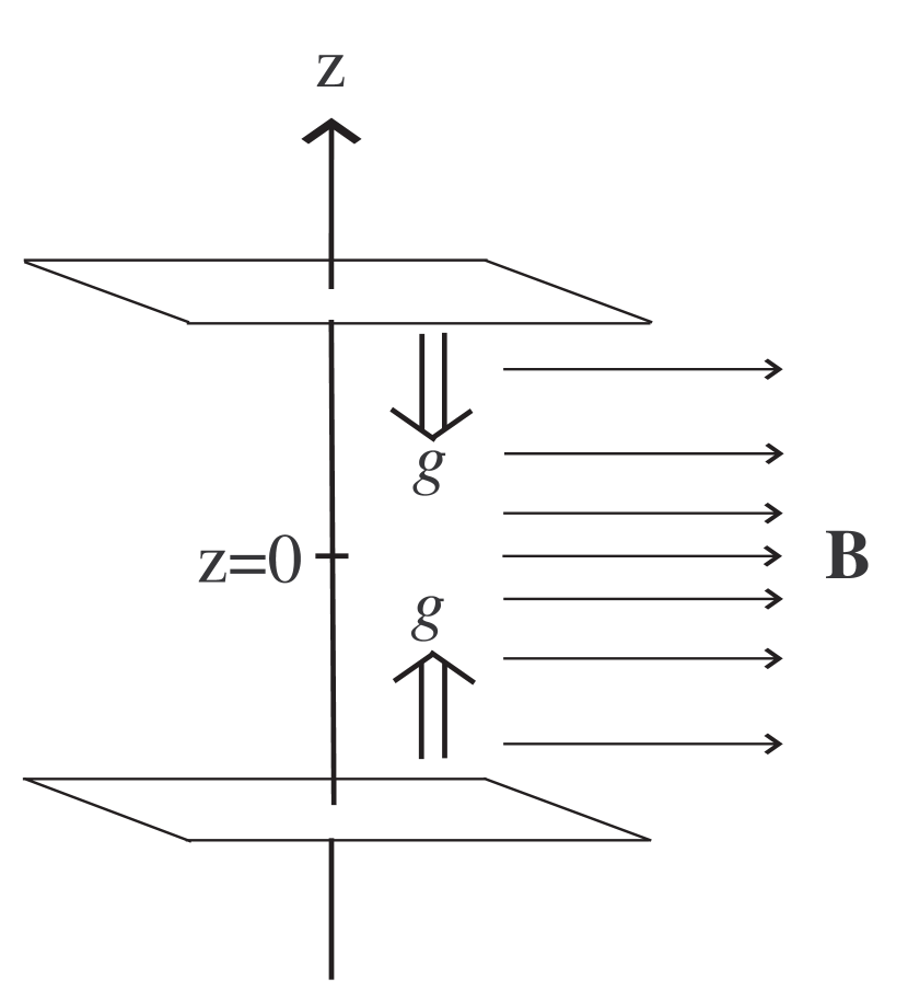
Figure 1: Schematic diagram of self-gravitating magnetic slab in $z$ direction.

We consider the evolution of a plane-parallel self-gravitating magnetized slab of lightly ionized molecular gas (see, Fig. 1). In this geometry, all variables are functions of distance $z$ to the central plane and time $t$ only. The magnetic field is frozen only to the ions, so that diffusion of the field relative to the neutral gas must continuously insert a drag force (per unit volume)

$$f_{d}=\gamma_{AD}\rho_{i}\rho v_{d},$$ (1)

where $\gamma_{AD}\sim 3.5\times 10^{10}\mathrm{m^{3}/kg.s}$ represents the collision drag coefficient and $\rho_{i}=\epsilon\rho^{\nu}$ is the ion density. In ionization equilibrium state $\nu=1/2$ and $\epsilon\sim 9.5\times 10^{-15}\mathrm{kg^{1/2}.m^{-3/2}}$ is valid, and $\nu\neq 1/2$ represents a deviation from equilibrium state (Shu 1992). The drift velocity is given by

$$v_{d}=-\frac{1}{\gamma_{AD}\epsilon\rho^{1+\nu}}\frac{\partial}{\partial z}(\frac{B^{2}}{2\mu_{0}}),$$ (2)

which is obtained by assumption that the pressure and gravitational force on the charged fluid component are negligible compared to the Lorentz force because of the low ionization fraction. In this way, the magnetic fields are directly evolved by charged fluid component, as follows:

$$\frac{dB}{dt}=-B\frac{\partial v}{\partial z}+\frac{\partial}{\partial z}(Bv_{d}).$$ (3)

Since the ion density is negligible in comparison to the neutral density, the mass conservation is given by

$$\frac{d\rho}{dt}=-\rho\frac{\partial v}{\partial z}.$$ (4)

The momentum equation then becomes

$$\frac{dv}{dt}=g-\frac{1}{\rho}\frac{\partial}{\partial z}(a^{2}\rho+\frac{B^{2}}{2\mu_{0}})$$ (5)

where $a$ is the isothermal sound speed and the gravitational acceleration $g$ obeys the poisson’s equation

$$\frac{\partial g}{\partial z}=-4\pi G\rho.$$ (6)

Following the many previous treatments, a further simplification is possible if we introduce the surface density between mid-plane and $z>0$ as

$$\sigma\equiv\int_{0}^{z}\rho(z^{\prime},t)dz^{\prime}.$$ (7)

The usual defined surface density from $-z$ to $+z$ has twice the value of $\sigma$. By transformation from $(z,t)$ to $(\sigma,t)$,

$$\frac{d}{dt}=\left(\frac{\partial}{\partial t}\right)_{\sigma},\quad\frac{\partial}{\partial z}=\rho\left(\frac{\partial}{\partial\sigma}\right)_{t},$$

the drift velocity is

$$v_{d}=-\frac{1}{\gamma_{AD}\epsilon\rho^{\nu}}\frac{\partial}{\partial\sigma}(\frac{B^{2}}{2\mu_{0}}),$$ (8)

and the equation (3) becomes

$$\frac{\partial}{\partial t}(\frac{B}{\rho})=\frac{1}{\gamma_{AD}\epsilon\mu_{0}}\frac{\partial}{\partial\sigma}(\frac{B^{2}}{\rho^{\nu}}\frac{\partial B}{\partial\sigma}).$$ (9)

With the above, field equation (6) can be integrated to give

$$g=-4\pi G\sigma,$$ (10)

while the equation of continuity (4) and the equation of motion (5) take the form

$$\frac{\partial z}{\partial\sigma}=\frac{1}{\rho}$$ (11)

and

$$\frac{\partial^{2}z}{\partial t^{2}}=-4\pi G\sigma-\frac{\partial}{\partial\sigma}(a^{2}\rho+\frac{B^{2}}{2\mu_{0}}),$$ (12)

respectively. The slab is assumed to be in quasi-magnetohydrostatic equilibrium at all time, supported against its own self-gravity by the magnetic nd gas pressure. The loss of flux from ambipolar diffusion is exactly compensated for by the compression of the slab which is necessary to maintain equilibrium. In this approximation, the left-hand side of equation (12) is zero, and we may integrate the force balance to obtain

$$\frac{B^{2}}{2\mu_{0}}+a^{2}\rho=2\pi G(\sigma_{\infty}^{2}-\sigma^{2})$$ (13)

where integration constant $\sigma_{\infty}$ is the value of $\sigma$ at $z=\infty$ (where $\rho$ is zero).

In a sense, our goal is to obtain the variation of drift velocity as a function of density at initial time. Evolution of the slab is beyond the scope of this paper. For this purpose, we follow the work of Shu (1983) to introduce the non-dimension quantities

$$\tilde{\sigma}\equiv\frac{\sigma}{\sigma_{\infty}},\quad\tilde{\rho}\equiv\frac{a^{2}}{2\pi G\sigma_{\infty}^{2}}\rho,\quad\tilde{z}\equiv\frac{2\pi G\sigma_{\infty}}{a^{2}}z,~{}~{}~{}~{}~{}$$

$$\tilde{B}\equiv\frac{B}{2\sigma_{\infty}\sqrt{\pi\mu_{0}G}},\quad\tilde{t}\equiv(\frac{2(2\pi G)^{1-\nu}}{\gamma_{AD}\epsilon})(\frac{2\pi G\sigma_{\infty}^{2-2\nu}}{a^{2-2\nu}})t,$$ (14)

so that we rewrite the basic equations (9), (11) and (13) as follows:

$$\frac{\partial}{\partial\tilde{t}}(\frac{\tilde{B}}{\tilde{\rho}})=\frac{\partial}{\partial\tilde{\sigma}}(\frac{\tilde{B}^{2}}{\tilde{\rho}^{\nu}}\frac{\partial\tilde{B}}{\partial\tilde{\sigma}}),$$ (15)

$$\tilde{B}^{2}+\tilde{\rho}=1-\tilde{\sigma}^{2},$$ (16)

$$\frac{\partial\tilde{z}}{\partial\tilde{\sigma}}=\frac{1}{\tilde{\rho}}.$$ (17)

In this way, a natural family of initial states is generated by assuming that the initial ratio of magnetic to gas pressure is everywhere a constant, $\alpha_{0}$, i.e., $\tilde{B}^{2}/\tilde{\rho}=\alpha_{0}$ at $\tilde{t}=0$. Then one finds from equations (16), (17) and (8) that

$$\rho_{(z,t=0)}=\frac{\rho_{0}}{\cosh^{2}(z/z_{\infty})},$$ (18)

$$v_{d}=\frac{2\alpha_{0}}{\sqrt{1+\alpha_{0}}}\frac{a\sqrt{2\pi G}}{\gamma_{AD}\epsilon\rho_{0}^{\nu-1/2}}\left(\frac{\rho_{(z,t=0)}}{\rho_{0}}\right)^{-\nu}\sqrt{1-\frac{\rho_{(z,t=0)}}{\rho_{0}}},$$ (19)

where $\rho_{0}\equiv 2\pi G\sigma_{\infty}^{2}/a^{2}(1+\alpha_{0})$ is the central density of the slab at $t=0$, and $z_{\infty}\equiv a\sqrt{(1+\alpha_{0})/2\pi G\rho_{0}}$ is a length-scale parameter.

The interior magnetic field of a molecular cloud acts only on the ions and electrons, so that the tendency for the field lines to straighten out is impeded by collisions of charged particles with the neutral particles. A simple physical derivation of the ambipolar drift heating rate ($\mathrm{J.kg^{-1}.s^{-1}}$) is given by considering the drag force (1) as follows

$$\Gamma_{AD}=\frac{\textbf{f}_{d}.\textbf{v}_{d}}{\rho}=\gamma_{AD}\epsilon\rho^{\nu}v_{d}^{2}.$$ (20)

Substituting the equations (18) and (19) into equation (20), the ambipolar drift heating rate of a molecular slab is given by

$$\Gamma_{AD}=\frac{\alpha_{0}^{2}}{1+\alpha_{0}}\frac{8\pi G}{\gamma_{AD}\epsilon}a^{2}\rho_{0}^{1-\nu}\frac{1-\rho/\rho_{0}}{(\rho/\rho_{0})^{\nu}},$$ (21)

which can be compared to the heating of cosmic rays (e.g., Goldsmith 2001),

$$\Gamma_{CR}\approx 3.12\times 10^{-8}\quad\mathrm{J.kg^{-1}.s^{-1}},$$ (22)

as follows ($\nu=1/2$)

$$\frac{\Gamma_{AD}}{\Gamma_{CR}}=\frac{\alpha_{0}^{2}}{1+\alpha_{0}}\left(\frac{a}{300\mathrm{m.s}^{-1}}\right)^{2}\left(\frac{n_{0}}{10^{12}\mathrm{m}^{-3}}\right)^{1/2}\frac{1-n/n_{0}}{(n/n_{0})^{1/2}}$$ (23)

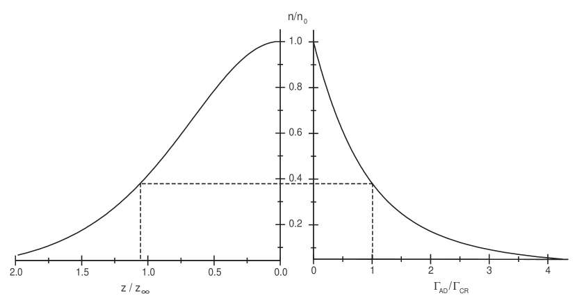
Figure 2: Relative magnitude of the ambipolar drift heating rate of a self-gravitating molecular slab in the case of $\alpha_{0}=1$, $a=0.3\mathrm{km.s^{-1}}$, and $n_{0}=10^{12}\mathrm{m^{-3}}$. The density profile of the slab is given for comparison.

that is shown in Fig. 2 for typical values of $\alpha_{0}=1$, $a=0.3\mathrm{km.s^{-1}}$, and $n_{0}=10^{12}\mathrm{m^{-3}}$. We have chosen to plot the density profile (18), because this makes it easy to compare the relative magnitude of ambipolar drift heating at different regions of the slab. Since the drift velocity is inversely proportional to the density (e.g., Eq.19), it is clear that the ambipolar drift heating rate is predominated in the outer regions of the slab.

It would also be interesting to derive a rough estimate of heating due to the drift induced by turbulent motions and to compare its order of magnitude with the heating of cosmic rays. Following Black (1987) the turbulence dissipation heating rate can be estimated as

$$\Gamma_{turb} \sim \frac{(\frac{1}{2}mv_{turb}^{2})(v_{turb}n)(\frac{1}{l})}{mn}$$ (24)

$$\sim 1.6\times 10^{-8}(\frac{v_{turb}}{1~{}\mathrm{km.s}^{-1}})^{3}(\frac{1~{}\mathrm{pc}}{l})\quad\mathrm{J.kg}^{-1}.\mathrm{s}^{-1},$$

where $v_{turb}$ is the turbulent velocity and $l$ is the dissipation length scale. With $v_{turb}\sim 1~{}\mathrm{km.s}^{-1}$ and $l\sim 1~{}\mathrm{pc}$, we calculate $\Gamma_{turb}\sim 1.6\times 10^{-8}\mathrm{J.kg}^{-1}.\mathrm{s}^{-1}$, comparable to half of the heating rate of cosmic rays (i.e., Eq. 22).

3 Isobaric Thermal Instability

3.1 The Molecular Gas Cooling Function

The cooling rate for molecular gas that is used in this work is based on the ”standard abundances” adopted by G01. I will briefly review here the important aspects of its construction. Calculation of thermal balance in molecular clouds by Goldsmith & Langer (1978), Neufeld et al. (1995), and G01 have shown that the various isotopic variants of the carbon mooxide molecule are certainly important coolants at high densities (i.e. $n\gtrsim 10^{10}\mathrm{m^{-3}}$). This is because the transitions that contribute to the cooling are thermalized due to the combination of higher collision rate and radiative trapping. The ”standard abundances” for ${}^{12}\mathrm{CO}$, ${}^{13}\mathrm{CO}$, and $\mathrm{C^{18}O}$ was adopted by G01 based on the observational data equal to $5.62\times 10^{-5}$, $1.00\times 10^{-6}$, and $1.00\times 10^{-7}$ relative to that of $\mathrm{H}_{2}$, respectively. Neutral Carbon is an important coolant since although it has only two fine structure transitions available, they have modest energies, and the abundance of this atom is relatively large.

The fractional abundances of ortho and para water vapor in molecular clouds are surprisingly low, so that G01 adopted a number density of ortho-$\mathrm{H}_{2}\mathrm{O}$ relative to that of $\mathrm{H}_{2}$ equal to $10^{-8}$. He have also doubled the ortho-$\mathrm{H}_{2}\mathrm{O}$ cooling rate to account approximately for contribution of para-$\mathrm{H}_{2}\mathrm{O}$. There is a large number of molecular species, including $\mathrm{CN}$, $\mathrm{HCN}$, $\mathrm{CS}$, $\mathrm{NH}_{3}$, $\mathrm{HCO}^{+}$, and $\mathrm{H}_{2}\mathrm{CO}$, that have low fractional abundances. To simplify the cooling calculation, G01 proposed the $\mathrm{CS}$ molecule as representative and multiplied its cooling by a factor of $10$ to include the contribution of the other species in this category.

The velocity field in molecular clouds is not well understood in detail. We can assume that the large velocity gradient approximation is valid for the radiative transfer calculations necessary to compute the molecular cooling when the optical depths are not small. A critical input to the large velocity gradient calculation is the molecular abundance per unit velocity gradient, which is equivalent to the column density per unit line width. Comparing the sizes and line widths for many clouds gives a characteristic value of $1~{}\mathrm{km.s}^{-1}.\mathrm{pc}^{-1}$ that was used by G01. The use of the large velocity gradient model introduces some uncertainty, but, do not significantly alter the total cooling rate.

In this way, the total cooling has a complicated dependence on the temperature and density of molecular hydrogen, parameterized by G01 as

$$\Lambda_{(n,T)}=\Lambda_{(n)}(\frac{T}{T_{0}})^{\beta(n)}\quad\mathrm{J.s^{-1}.kg^{-1}},$$ (25)

where $T_{0}=10\mathrm{K}$ and the values of $\Lambda(n)$ and $\beta(n)$ are given in Table 1 for standard abundances and velocity gradient of $1~{}\mathrm{km.s}^{-1}.\mathrm{pc}^{-1}$. Here, we use the polynomial fitting functions as follows

$$\log\left(\frac{\Lambda_{(n)}}{\mathrm{J.kg^{-1}.s^{-1}}}\right)=-8.98-0.87(\log\frac{n}{n_{0}})-0.14(\log\frac{n}{n_{0}})^{2},$$ (26)

$$\beta_{(n)}=3.07-0.11(\log\frac{n}{n_{0}})-0.13(\log\frac{n}{n_{0}})^{2},$$ (27)

where $n_{0}=10^{12}\mathrm{m^{-3}}$. Another expression for the parameter $\Lambda_{(n)}$ is

$$\log\Lambda_{(n)}=\log\Lambda_{0}+\delta\log\frac{n}{n_{0}},$$ (28)

which was used by Nejad-Asghar & Ghanbari (2003, 2006) and SLH, for linear investigation of thermal instability in a narrow range of density. In this formalism, the approximate values of $\Lambda_{0}$ and $\delta$ between neighbor densities are given in Table 1.

There is observational evidences that a variety of molecular species are depleted on the surface of dust grains (e.g., Tielen & Whittet 1997). The observational results on depletion of different species are relatively limited and are certainly compromised by blending of emission from different regions along the line of sight. It is quite difficult to know exactly how the column densities or abundances of species observed on dust grain surfaces are related to the abundances in the gas phase. There also have not been systematic studies of the depletion of a wide range of molecular species in a set of sources. In this way, G01 used the fragmentary data from a selection of clouds to analyze the effects of molecular depletion on the standard values of the cooling function parameters $\Lambda(n)$ and $\beta_{(n)}$. Because of the above mentioned uncertainties, we should treat the cooling function in a parametric fashion with $\Lambda(n)$ and $\beta_{(n)}$ approximately near the standard values of Table 1.

The cooling function was constructed assuming that statistical steady-state equilibrium is valid, so that the chemical times are very short with respect to dynamical and cooling times. For all of the trace coolants this is reasonable except $\mathrm{H}_{2}$ molecule that the collision time (time to reach statistical steady-state equilibrium) is necessarily of order the cooling time (Gilden 1984). The $\mathrm{H}_{2}$ is the main coolant at higher temperatures (the temperature where the carbon monoxide and $\mathrm{H}_{2}$ contribute equally is slowly increasing function of density). At the very low temperatures of interest considered by G01 in the molecular clouds, $\mathrm{H}_{2}$ do not play a significant role as a major coolant because of its low-lying energy levels. Thus, the standard values of the cooling function parameters $\Lambda(n)$ and $\beta_{(n)}$ (as mentioned in Table 1) based on the statistical steady-state equilibrium are approximately appropriate for our analysis.

Models of the molecular clouds identify several different heating mechanisms. Here, we use the heating of cosmic ray (22) and the ion-neutral slip heating rate as described by equation (23). The isobaric instability mode in a thermal equilibrium gas can be discussed in relation to the two-phase model in the same way as described in figure 3 of Gilden (1984). The detailed study of the linear investigation and dynamical evolution of the isobaric modes are given in the next sub-section. The instance here can be analyzed in a graphical approach. The pressure-density plane is an elegant method to describe the isobaric instability modes in the thermal equilibrium,

$$\Lambda_{(n)}(\frac{T}{T_{0}})^{\beta(n)}=\Gamma_{CR}+\Gamma_{AD},$$ (29)

of a molecular gas. Substituting the equation (23) into (29), the pressure in thermal equilibrium self-gravitating molecular slab can be obtained as

$$\frac{p}{p_{0}} = \frac{nT}{n_{0}T_{0}}$$ (30)

$$= (\frac{n}{n_{0}})\left\{\frac{\Gamma_{CR}}{\Lambda_{(n)}}\left[1+\frac{\alpha_{0}^{2}}{1+\alpha_{0}}(\frac{a}{300\mathrm{m.s}^{-1}})^{2}(\frac{n_{0}}{10^{12}\mathrm{m}^{-3}})^{1/2}\frac{1-n/n_{0}}{(n/n_{0})^{1/2}}\right]\right\}^{1/\beta(n)}.$$

The two-phase instability is displayed in Fig. 3 where the values of $a$ and $n_{0}$ are typically chosen equal to $0.3\mathrm{km.s^{-1}}$ and $10^{12}\mathrm{m^{-3}}$, respectively. The diagram of Fig. 3 shows the equilibrium state without magnetic field (i.e., $\alpha_{0}=0$) in comparison with considering of the ambipolar drift heating rate with $\alpha_{0}=10$. This figure suggests that without ambipolar diffusion friction, there would not be isobaric thermal instability. This is not what has been found by Gilden (1984), because as we known the thermal instability is very sensitive to the net cooling function. Here we use the approximately most accurate cooling function which is evaluated by G0. An equilibrium state is specified by the intersection of a thermal equilibrium curve and a constant pressure line. The two curves in Fig. 3 display that considering of ambipolar drift heating rate causes to bifurcate the slab into two phases, with individual gas elements going into that phase corresponding to the sign of the initial fluctuation.

3.2 Condensation Growth

Equation (19) shows that the drift velocity is inversely proportional to the density so that we can choose, in a general form, $v_{d}=\mathrm{const.}\times\rho^{-b}$ where $b>0$. For a self-gravitating slab, the value of $b$ may be approximated roughly between $0.5$ to $2.0$. This range of values should be compared to equation (10) of Nejad-Asghar & Ghanbari (2006), where $b=1+\nu$ was used. The heating due to ion-neutral friction is spatially dependent (because it depends on gas density and gas density varies with position). Here we do not consider this issue in the instability analysis because we are interested considering the AU-scale condensations that may be formed from waves with small wavelengths (respect to the cloud size). In this formalism, equation (37) of SLH for isobaric thermal instability may be generalized to

$$\lambda_{c1}=\frac{\lambda_{0}}{\sqrt{\frac{\delta+(2b-\nu)\xi}{\beta}-1}}$$ (31)

with $\xi\equiv\Gamma_{AD}/\Lambda$ and $\lambda_{0}\equiv 2\pi\sqrt{KT/\rho\beta\Lambda}$ where $K$ is the thermal conduction coefficient. If the wavelength of perturbation is larger than the critical wavelength (31), there will occur isobaric instability. This requires

$$\delta+(2b-\nu)\xi>\beta.$$ (32)

Since $0<\xi<1$, we find that

$$\delta>\beta-(2b-\nu)$$ (33)

is required for occurrence of isobaric thermal instability. On the other hand, critical wavelength of isentropic thermal instability (equation 38 of SLH) is modified as

$$\lambda_{c2}=\frac{\lambda_{0}}{\sqrt{-\frac{3}{2}\frac{\delta-(2b-\nu)\xi}{\beta}-1}},$$ (34)

which requires

$$\delta<-\frac{2}{3}\beta-(2b-\nu)\xi.$$ (35)

Thus, the condition

$$\delta<-\frac{2}{3}\beta$$ (36)

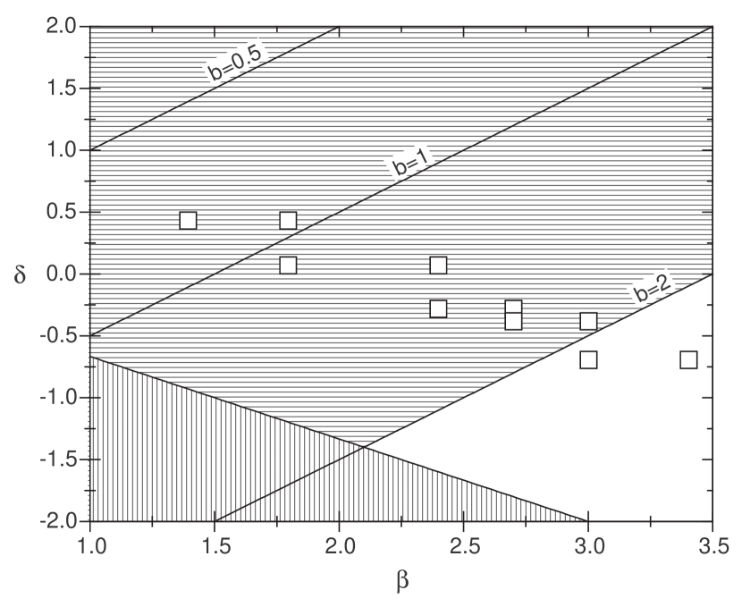
Figure 4: Isobaric (horizontal shade) and isentropic (vertical shade) thermal instability regimes in terms of temperature dependence $\beta$ and density dependence $\delta$ in the parameterized cooling function. The squares $\Box$ represent the values of $\beta$ and $\delta$ from table 1.

must at least be held for occurrence of isentropic thermal instability. The instability regimes are summarized in Fig. 4. Depending on the chosen density range, the values of $\beta$ and $\delta$ can differ, but we can only expect the isobaric thermal instability mode. The isentropic regime can not be fulfilled in the molecular slab. Therefore, we only consider the nonlinear isobaric thermal instability mode.

To give a complete description of the nonlinear thermal runaway, one needs to solve the nonlinear fluid equations. The energy equation follows from the use of the first law of thermodynamics, that is

$$\frac{1}{\gamma-1}\frac{dp}{dt}-\frac{\gamma}{\gamma-1}\frac{p}{\rho}\frac{d\rho}{dt}+\rho\Omega_{(\rho,T)}=0,$$ (37)

where $\gamma$ is the polytropic index, $\Omega_{(\rho,T)}$ is the net cooling function

$$\Omega_{(\rho,T)}\equiv\Lambda_{(\rho,T)}-(\Gamma_{CR}+\Gamma_{AD}),$$ (38)

and the pressure $p$ is given by the ideal gas equation of state

$$p=\frac{R}{\mu}\rho T,$$ (39)

where $\mu$ is the mean atomic mass per particle and $R$ is the universal gas constant. Being interested in the development of the isobaric thermal instability in the quasi-hydrostatic molecular slab, we put $dp/dt=0$ in the energy equation (37) and obtain the following equation

$$\frac{dT}{dt}+\frac{\gamma-1}{\gamma}\frac{\mu}{R}\Omega_{(T,z)}=0,$$ (40)

where the isobaric condition $\rho\propto T^{-1}$ is used. Now let us introduce the dimensionless temperature, $\tilde{T}\equiv T/T_{0}$, to present the energy equation (40) as dimensionless form

$$\frac{\partial\tilde{T}}{\partial\tilde{t}}+\tilde{\Omega}_{(\tilde{T},\tilde{z})}=0$$ (41)

where $\tilde{\Omega}_{(\tilde{T},\tilde{z})}$ is the dimensionless net cooling function of the slab

$$\tilde{\Omega}_{(\tilde{T},\tilde{z})}\equiv(\frac{\gamma-1}{\gamma}\frac{\mu}{R}\frac{1}{T_{0}})(\frac{\gamma_{AD}\epsilon}{2(2\pi G)^{1-\nu}})(\frac{a^{2-2\nu}}{2\pi G\sigma_{\infty}^{2-2\nu}})\Omega_{(T,z)}.$$ (42)

Thus, the nonlinear dynamics of the isobaric thermal instability is determined solely by the form of the net cooling function curve $\tilde{\Omega}_{(\tilde{T},\tilde{z})}$ and the initial conditions in the equation (41). We use the equations (21), (22), and (25)-(27) to find the net cooling function of a self-gravitating molecular slab. Figure 5 shows the net cooling function of the slab for typical values of $\tilde{T}_{(\tilde{t}=0)}$. The necessary condition for the instability has the form $d\tilde{\Omega}/d\tilde{n}>0$, which in the slab can be expressed as $d\tilde{\Omega}/d\tilde{z}<0$. This condition can be easily seen to be fulfilled with the equilibrium points $u_{1}$ and $u_{2}$ in the Fig. 5. Indeed, these results accurately coincide with the linear instability regimes that are summarized in Fig. 3. We consider a constant initial form of the temperature profile in the slab, and solve numerically the temperature equation (41) with approximation that the dynamics of the slab is solely determined by the equations (15)-(17) and the initial condition (18) as outlined by Shu (1983). Figure 6 gives a plot of the evolution of the temperature profile in a typical case described in Fig. 5. As can be seen in Fig. 6, large temperature gradients are created with time at the interfaces between different unstable thermal phases.

4 Summary and Conclusion

In this paper the importance of ambipolar drift heating rate on net cooling function have been investigated, and the isobaric thermal instability in a self-gravitating magnetized molecular slab is analyzed. We re-formulate the equations of a quasi-magnetohydrostatic self-gravitation slab so that the density dependence of the drift velocity is estimated. Since the drift velocity is inversely proportional to the density, the ambipolar drift heating rate is predominated in the outer regions of the slab.

Choosing a parametric density dependence of drift velocity, the isentropic and isobaric thermal instability criteria of SLH are generalized. We have applied the cooling rate of G01 to find the physical contents of the instability criteria. We have found that the isentropic thermal instability can not occur in the molecular cloud, while the isobaric criteria is accurately complied. This term is also investigated by considering of thermal equilibrium in pressure-density plane, and by plotting of the net cooling function in Fig. 5.

We have considered a constant initial form of the temperature profile in the slab, and have solved numerically the nonlinear isobaric energy equation with approximation that the dynamics of the slab is solely determined by the isothermal equations as outlined by Shu (1983). In this way, a large temperature gradient are created with time at the interfaces between different isobaric unstable thermal phases. In the context of our thermal instability analysis in the molecular slab, we find that the isobaric thermal instability can occur in some regions of it, therefore it may produce the slab fragmentation and formation of the spherical AU-scale condensations.

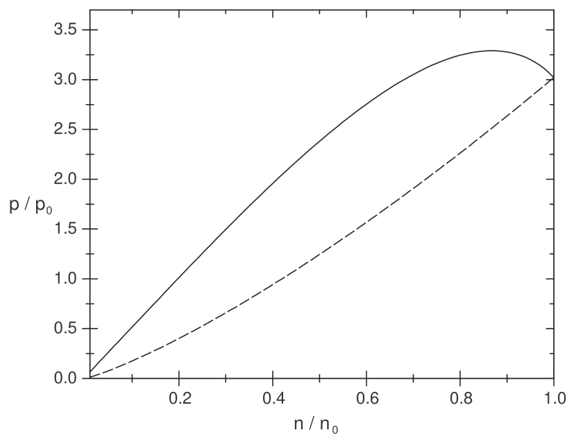
Figure 3: Curves of thermal equilibrium in the pressure-density plane. The dash curve represents the equilibrium state without magnetic field (i.e., $\alpha_{0}=0$), and the solid curve is obtained by considering the ambipolar drift heating rate with $\alpha_{0}=10$, $a=0.3\mathrm{km.s^{-1}}$, and $n_{0}=10^{12}\mathrm{m^{-3}}$.

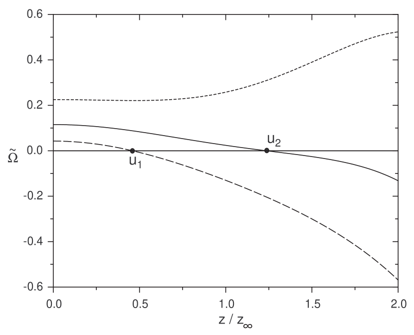
Figure 5: The non-dimensional net cooling function of the self-gravitating slab with $\alpha_{0}=10$, $a=0.3\mathrm{km.s^{-1}}$, and $n_{0}=10^{12}\mathrm{m^{-3}}$ for cases $\tilde{T}_{(\tilde{t}=0)}=4$ (dash), $5$ (solid), and $6$ (dot). The points $u_{1}$ and $u_{2}$ are unstable because of $d\tilde{\Omega}/d\tilde{z}<0$.

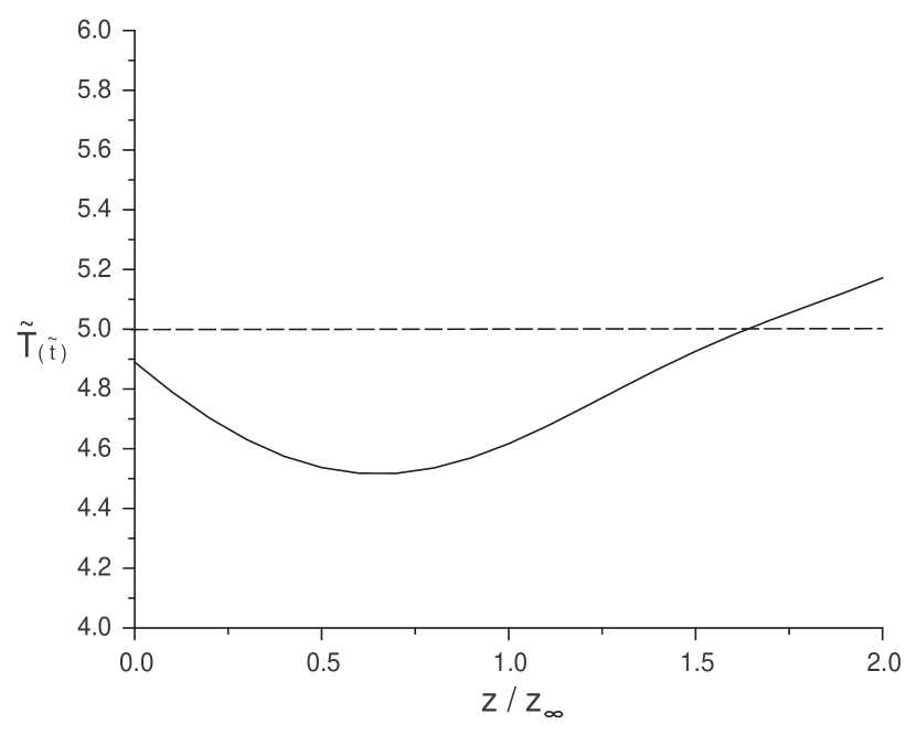
Figure 6: Evolution of the temperature of the isobaric unstable regions in self-gravitating molecular slab with $\alpha_{0}=10$, $a=0.3\mathrm{km.s^{-1}}$, and $n_{0}=10^{12}\mathrm{m^{-3}}$ from initial value $\tilde{T}=5$ at $\tilde{t}=0$ (dash) to a typical time $\tilde{t}=1$ (solid).

Table 1: Parameters for the gas cooling function with standard abundances and velocity gradient of $1~{}\mathrm{km.s}^{-1}.\mathrm{pc}^{-1}$.

$\log(\frac{n}{n_{0}})$	$\log(\frac{\Lambda_{(n)}}{\mathrm{J.kg^{-1}.s^{-1}}})$	$\beta_{(n)}$	$\log(\frac{\Lambda_{0}}{\mathrm{J.kg^{-1}.s^{-1}}})$	$\delta$
-4	-7.82	1.4
			$\}\Rightarrow$ -6.14	0.42
-3.5	-7.61	1.8
			$\}\Rightarrow$ -7.40	0.06
-3	-7.58	2.4
			$\}\Rightarrow$ -8.45	-0.29
-2	-7.87	2.7
			$\}\Rightarrow$ -8.65	-0.39
-1	-8.26	3.0
			$\}\Rightarrow$ -8.96	-0.7
0	-8.96	3.4

References

- (1) Audit, E., Hennebelle, P., 2005, A&A, 433, 1
- (2) Birk, G.T., 2000, Phys. Plasma, 7, 3811
- (3) Black, J.H., 1987, in Interstellar Processes, ed. Hollenbach, D.J., Thronsen, H.A., D. Reidel Publishing Company, p. 731
- (4) Boissé, P. Le Petit, F., Rollinde, E., Roueff, E., Pineau des Forêts, G., Andersson, B.G., Gry, C., Felenbok, P., 2005, A&A, 429, 509
- (5) Dickman, R.L., Horvath, M.A., Margulis, M., 1990, ApJ, 365, 586
- (6) Falgarone, E., Hily-Blant, P., Levrier, F., 2004, Ap&SS, 292, 89
- (7) Falle, S.A.E.G., Hartquist, T.W., 2002, MNRAS, 329, 195
- (8) Folini, D., Heyvaerts, J., Walder, R., 2004, A&A, 414, 559
- (9) Gammie, C.F., Ostriker, E.C., 1996, ApJ, 466, 814
- (10) Gilden, D.L., 1984, ApJ, 283, 679
- (11) Goldsmith, P.F., 2001, ApJ, 557, 736 (G01)
- (12) Goldsmith, P.F., Langer, W.D., 1978, ApJ, 222, 881
- (13) Heitsch, F., Slyz, A.D., Devriendt, J.E.G., Hartmann, L.W., Burkert, A., 2006, ApJ, 648, 1052
- (14) Hennebelle, P., Passot, T., 2006, A&A, 448, 1083
- (15) Hennebelle, P., Peráult, M., 2000, A&A, 359, 1124
- (16) Inoue, T., Inutsuka, S., Koyama, H., 2007, ApJ, 658, 99
- (17) Koyama, H., Inutsuka, S., 2002, ApJ, 564, 97
- (18) Kwan, J., 1979, ApJ, 229, 567
- (19) Kwan, J., Sanders, D.B., 1986, ApJ, 309, 783
- (20) Liszt, H., Lucas, R., 2000, A&A, 355, 333
- (21) Loewenstein, M., 1990, ApJ, 349, 471
- (22) Marscher, A.P., Moore, E.M., Bania, T.M., 1993, ApJ, 419, 101
- (23) Moore, E.M., Marscher, A.P., 1995, ApJ, 452, 679
- (24) Murray, S.D., Lin, D.N.C., 1996, ApJ, 467, 728
- (25) Nejad-Asghar, M., Ghanbari, J., 2003, 2003, MNRAS, 345, 1323
- (26) Nejad-Asghar, M., Ghanbari, J., 2006, Ap&SS, 302, 243
- (27) Neufeld, D.A., Leep, S., Melnick, G.J., 1995, ApJS, 100, 132
- (28) Pan, K., Federman, S.R., Welty, D.E., 2001, ApJ, 558, 105
- (29) Perault, M., Falgarone, E., Puget, J.L., 1985, A&A, 152, 371
- (30) Pringle, J.E., Allen, R.J., Lubow, S.H., 2001, MNRAS, 327, 663
- (31) Rollinde, E., Boissé, P., Federman, S.R., Pan, K., 2003, A&A, 401, 215
- (32) Shu, F., 1983, ApJ, 273, 202
- (33) Shu, F., 1992, The Physics of Astrophysics, University Science Books, Mill Valley, CA., Vol II., p. 360
- (34) Silk, J., Takahashi, T., 1979, ApJ, 229, 242
- (35) Steele, C.D.,C., Ibáñez S., M.H., 1999, Phys. Plasma, 6, 3086
- (36) Stiele, H., Lesch, H., Heitsch, F., 2006, MNRAS, 372, 862 (SLH)
- (37) Tielens, A.G.G.M., Whittet, D.C.B., 1997, IAU Symp. 178, Molecules in Astrophysics: Probes and Processes, ed. van Dishoeck, E.F., Dordrecht: Kluwer, 45
- (38) Thoraval, S., Boissé, P., Stark, R., 1996, A&A, 973, 312
- (39) Vazquez-Semadeni, E., Ryu, D., Passot, T., González, R.F., Gazol, A., 2006, ApJ, 643, 245
- (40) Williams, J.P., Blitz, L., McKee, C.F., 2000, in Protostars and Planets IV, ed. Mannings, V., Boss, A.P., Russel, S.S., Tucson: University of Arizona Press, p. 97