Characterizing Potentials by a Generalized Boltzmann Factor

Abstract

Based on the concept of a nonequilibrium steady state, we present a novel method to experimentally determine energy landscapes acting on colloidal systems. By measuring the stationary probability distribution and the current in the system, we explore potential landscapes with barriers up to several hundred $\mathit{k_{\mathrm{B}}T}$. As an illustration, we use this approach to measure the effective diffusion coefficient of a colloidal particle moving in a tilted potential.

Introduction. – The interaction of soft matter systems with potential landscapes created by optical tweezers plays a key role for, e.g., mechanical flexibility measurements of single biomolecules or molecular motors meh99 ; wan97 , guiding of neuronal cells ehr02 , or phase transitions of colloidal monolayers on patterned substrates man03 ; bru02 . In addition, extended optical lattices can be used as sorters for microscopic particles don03 or as microoptomechanical devices such as Couette rheometers lad05 . Currently, no theories are available which can be used to directly calculate optical trapping forces on macromolecules. Thus the precise calibration of optical forces is a central issue in many experiments.

The simplest method to determine an optical potential $V(\mathbf{r})$ is to measure the equilibrium distribution $p_{\mathrm{eq}}(\mathbf{r})$ of a highly diluted colloidal system at position $\mathbf{r}$. From the inverted Boltzmann factor

$$V(\mathbf{r})=-\mathit{k_{\mathrm{B}}T}\ln p_{\mathrm{eq}}(\mathbf{r})$$ (1)

one directly obtains the underlying potential $V(\mathbf{r})$ with a typical energy resolution on the order of $0.1\,\mathit{k_{\mathrm{B}}T}$ roh04 ; man03 , where $k_{\mathrm{B}}$ is Boltzmann’s constant and $T$ the temperature of the surrounding fluid. This technique, however, is only applicable to potential depths up to $\simeq 7\,\mathit{k_{\mathrm{B}}T}$ which are effectively sampled by Brownian particles in equilibrium. For larger trapping potentials, optical forces are typically calibrated indirectly by taking advantage of Stokes law which relates the particle velocity to the friction force exerted by the surrounding solvent molecules. Accordingly, from the drift velocity of a particle, the underlying potential can be reconstructed  fauc95 ; pou97 ; ska06 . Alternatively, within the drag force method, $V(\mathbf{r})$ can be determined from the particle’s displacement upon moving the sample stage (and thus the liquid) with known velocity wan97 ; meh99 ; she98 ; ghi94 . In contrast to Eq. (1), however, the latter two nonequilibrium methods neglect thermal fluctuations since only mean values of particle velocities or displacements are considered. While such fluctuations can be neglected at large trapping forces, this is no longer justified for external forces with strengths comparable to those exerted by fluctuating Brownian forces.

In this paper, we introduce a potential reconstruction method based on a generalization of Eq. (1) to nonequilibrium conditions. This is experimentally realized by generating a nonequilibrium steady state (NESS) for a colloidal particle in a one-dimensional (toroidal) potential landscape. By measuring the stationary probability distribution and the current in the system, we can reliably calibrate potentials wells between a few tens up to several hundreds of $\mathit{k_{\mathrm{B}}T}$.

Potential reconstruction. – Our method is based on a generalization of the Boltzmann factor inversion (1) to nonequilibrium. The effectively one-dimensional motion of the particle along a toroidal trap is governed by a Langevin equation

$$\dot{x}=\gamma^{-1}F(x)+\zeta(t)$$ (2)

with $x$ the spatial coordinate and $\zeta(t)$ representing thermal noise with correlations $\langle\zeta(t)\zeta(t^{\prime})\rangle=2(\mathit{k_{\mathrm{B}}T}/\gamma)\delta(t-t^{\prime})$, where $\gamma$ is the friction coefficient. The force $F(x)=-V^{\prime}(x)+f$ exerted on the particle stems from two sources, the gradient of the periodic potential $V(x+L)=V(x)$ and a nonconservative driving force $f$.

We define a pseudo-”potential” $\phi(x)$ by writing the nonequilibrium steady state probability distribution as $p_{\mathrm{s}}(x)=\exp[-\phi(x)]$ resembling the Boltzmann factor. The stationary probability current through the toroid is given as

$$j_{\mathrm{s}}=\gamma^{-1}\left[F(x)p_{\mathrm{s}}(x)-\mathit{k_{\mathrm{B}}T}p_{\mathrm{s}}^{\prime}(x)\right],$$ (3)

which is constant in one dimension. We introduce the local mean velocity

$$v_{\mathrm{s}}(x)=j_{\mathrm{s}}/p_{\mathrm{s}}(x)$$

and obtain spec06

$$\gamma v_{\mathrm{s}}(x)=F(x)+\mathit{k_{\mathrm{B}}T}\phi^{\prime}(x)=-V^{\prime}(x)+f+\mathit{k_{\mathrm{B}}T}\phi^{\prime}(x).$$ (4)

Integration of Eq. (4) leads to the potential

$$V(x)=\mathit{k_{\mathrm{B}}T}\phi(x)+\int_{0}^{x}[f-\gamma v_{\mathrm{s}}(x)]dx$$ (5)

up to an irrelevant additive constant. Using the definitions of $\phi(x)$ and $v_{\mathrm{s}}(x)$ we finally arrive at

$$V(x)=-\mathit{k_{\mathrm{B}}T}\ln p_{\mathrm{s}}(x)+fx-\gamma j_{\mathrm{s}}\int_{0}^{x}p_{\mathrm{s}}^{-1}(x)dx.$$ (6)

Hence, the stationary probability $p_{\mathrm{s}}(x)$ and the local mean velocity $v_{\mathrm{s}}(x)$ determine the potential $V(x)$. The driving force $f$ can be determined by setting $x=L$ in Eq. (5) and using the periodicity of the potentials $V(x)$ and $\phi(x)$ as

$$f=\frac{\gamma}{L}\int_{0}^{L}v_{\mathrm{s}}(x)dx.$$ (7)

In thermal equilibrium both $j_{\mathrm{s}}$ and $f$ vanish and Eq. (6) reduces to the inverted Boltzmann factor Eq. (1). Therefore Eq. (6) can be understood as an extension of the Boltzmann factor to nonequilibrium stationary states.

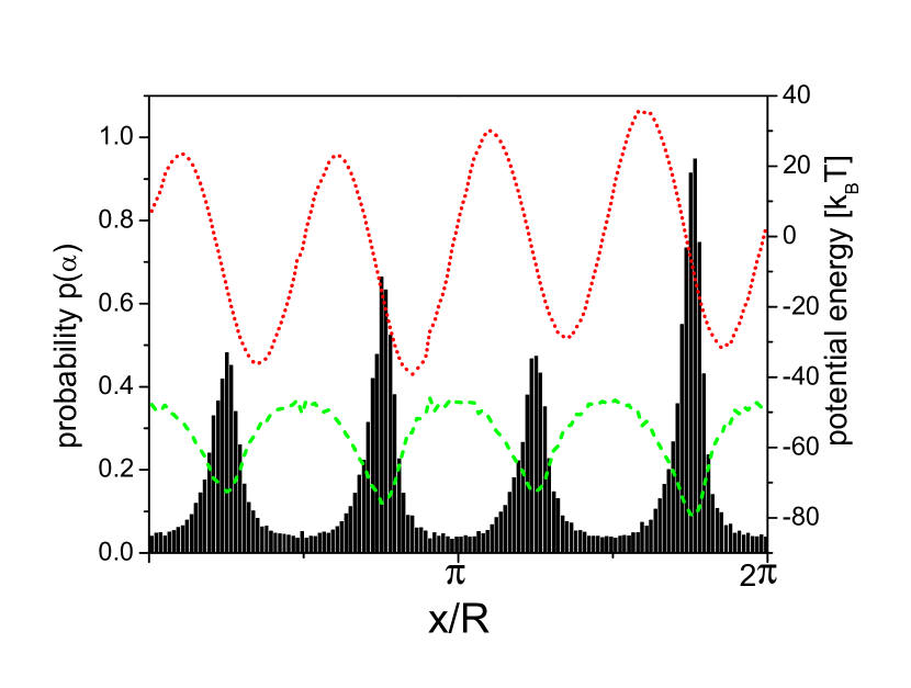
Figure 1: (color online) Stationary probability distribution $p_{\mathrm{s}}(x)$ (black bars) and the pseudopotential $\phi(x)$ (dashed line), measured at a driving force of $34\,\mathrm{\mathit{k_{\mathrm{B}}T}/\mu m}$, pointing along the negative x-direction. The potential $V(x)$ (dotted line) is determined according to Eq. (6). Note that $\phi(x)$is multiplied by a factor of 10 and shifted vertically to enhance visualization.

Experiment. – For an experiment exploiting Eq. (6), we use a scanning optical tweezers setup as described in detail elsewhere lutz06 . A laser beam ($\lambda\simeq 532\,\mathrm{nm}$) is deflected on a pair of galvanometric mirrors and focused with a 100x, NA=1.3 oil immersion objective from below onto a silica bead immersed in water (diameter $d\simeq 1.85\,\mathrm{\mu m}$). Upon periodic modulation of the angular mirror positions we obtain a three dimensional toroidal laser trap with a torus radius of $R\simeq 3.95\,\mathrm{\mu m}$. At our driving frequencies $\nu_{\mathrm{T}}\simeq 100\,\mathrm{Hz}$, the particle can not follow directly the rotating laser trap. Instead, every time the particle is passed by the laser tweezers, it experiences a minute kick along the rotation direction whose strength depends on the laser intensity $I_{0}$ fauc95 . Because the particle s trajectory is monitored with video microscopy at a sampling rate of $20\,\mathrm{Hz}$, single kicking events are not resolved and the driving force $f$ along the angular direction can be considered as constant lutz06 . In addition, the intensity of the laser is weakly modulated along the toroidal trap. This is achieved with an electro-optical modulator (EOM) being controlled by a function generator which is synchronized with the scanning motion of the mirrors. This intensity modulation $I_{m}(x)$ leads to a periodic potential $V(x)$ with $x$ the arc-length coordinate along the circumference of the torus. It has been demonstrated that the resulting optical forces of such an intensity modulated scanned laser tweezers exerted on a colloidal particle correspond to those of a tilted periodic potential  lutz06 .

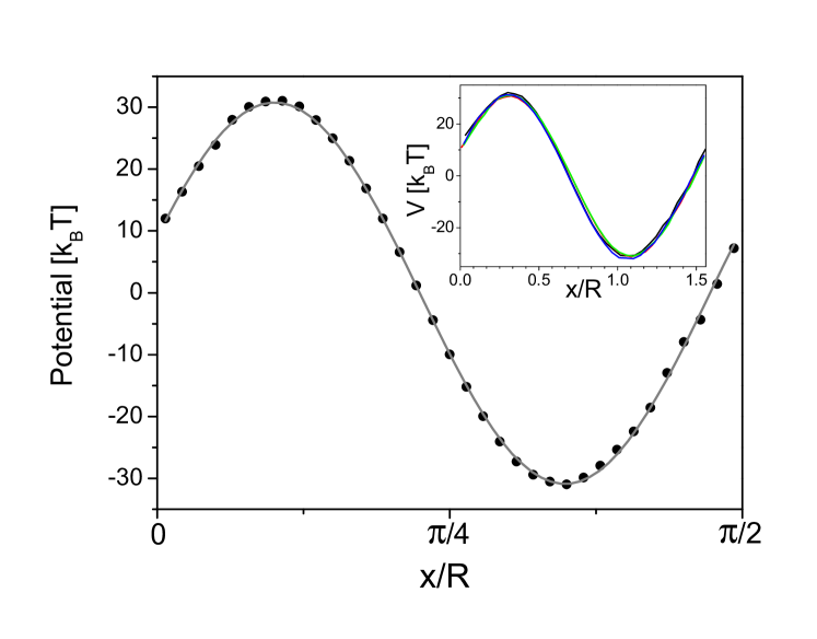
Figure 2: (color online) Averaged potential (solid points). The grey curve is a fit of Eq. (9) to the averaged potential. Inset: Averaged potentials obtained for driving forces $f$ ($=34$, $43$, $57$ and $73\,\mathrm{\mathit{k_{\mathrm{B}}T}/\mu m}$).

To experimentally demonstrate that $V(x)$ can be obtained under non-equilibrium steady state conditions, the intensity of the scanned laser tweezer along the toroidal trap was varied according to

$$I(x)=I_{0}+I_{m}\sin(n\frac{2\pi x}{L}).\hskip 19.91684pt(n=4)$$ (8)

Fig. 1 shows the steady state probability distribution $p_{\mathrm{s}}(x)$ as obtained from the particle s trajectory and the corresponding pseudo-potential $\phi(x)$ for $I_{0}=44\,\mathrm{mW}$ and $I_{m}=10\,\mathrm{mW}$. Together with the driving force $f=34\,\mathrm{\mathit{k_{\mathrm{B}}T}/\mu m}$ as determined from the measured local mean velocity $v_{\mathrm{s}}(x)$ (cf. Eq. (7)) we finally arrive at the potential $V(x)$ which is also plotted in Fig. 1 as dotted line. Clearly, under NESS conditions the minima and maxima of $\phi(x)$ and $V(x)$ do not coincide. In addition, $\phi(x)$ varies in a less pronounced way than $V(x)$ because $p_{\mathrm{s}}(x)$ is broader than it would be in equilibrium. On top of the intensity modulation according to Eq. (8) we observe a constant, small variation of the potential with $2\pi$-periodicity caused by minute optical distortions in our setup. Since we are only interested in the local shape of the potential, in the following we only consider potentials, where $V(x)$ is averaged over the four externally applied periods. The averaged potential, which is plotted as solid bullets in Fig. 2, is in excellent agreement with a sinusoidal fit to

$$V(x)=\frac{V_{0}}{2}\sin(4\frac{2\pi x}{L})$$ (9)

as theoretically expected for the optical potential in case of sinusoidal intensity variations tlu98 .

To demonstrate the robustness of our approach in characterizing equilibrium potentials under NESS conditions, we systematically varied the driving force $f=34$, $43$, $57$ and $73\,\mathrm{\mathit{k_{\mathrm{B}}T}/\mu m}$ while keeping $V(x)$ unchanged. Experimentally, this is achieved by changing $I_{0}$ with all other parameters in Eq. (8) fixed. The measured potentials plotted in the inset of Fig. 2 clearly fall on top of each other and thus demonstrate that the measured $V(x)$ is independent of $f$.

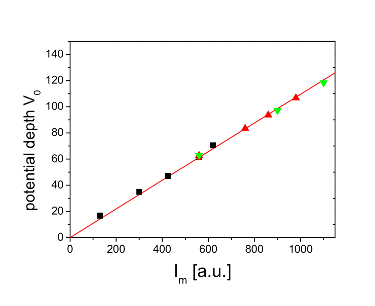
Figure 3: (color online) Potential depth as a function of the modulation amplitude $I_{m}$. The different symbols correspond to data acquired at different driving forces. ($\blacksquare$:$43$, $\blacktriangle$:$57$ and $\blacktriangledown$:$73\,\mathrm{\mathit{k_{\mathrm{B}}T}/\mu m}$)

Similarly, the potential amplitude $V_{0}$ can be changed by variation of $I_{m}$. Fig. 3 shows the potential depth as a function of $I_{m}$, measured at different driving forces $f$ (marked by different symbols). As expected, we find a linear dependence between $V_{0}$ and $I_{m}$ independent of $f$. This shows that reconstruction of equilibrium potentials can be reliably performed for a wide range of driving forces. For practical purposes, however, the driving force should not exceed a certain range where the lower limit is reached when the particle only rarely surmounts adjacent potential barriers and thus cannot sample the entire landscape. For very large $f$, the probability distribution becomes rather flat and very long sampling times are required to accurately measure $V(x)$.

Diffusion in tilted periodic potentials. – Having demonstrated the validity of our approach to reconstruct equilibrium potentials under NESS conditions, in the following we will exemplarily apply this method to the problem of giant diffusion. It has been shown theoretically rei01 and experimentally lee06 ; tat03 that the effective diffusion coefficient $D_{\mathrm{eff}}$ of a Brownian particle moving in a tilted periodic potential $U(x)=V(x)+fx$ exhibits a pronounced maximum as a function of the driving force $f$. Until now experiments were not able to match quantitatively the theoretical predictions. With the ability to characterize the underlying potential landscape in detail, we can quantitatively test the theoretical behavior of $D_{\mathrm{eff}}$.

The effective diffusion coefficient is easily obtained from the particle trajectory according to

$$D_{\mathrm{eff}}=\lim_{t\rightarrow\infty}D(t),\qquad D(t)=\frac{\langle x(t)^{2}\rangle-\langle x(t)\rangle^{2}}{2t}.$$ (10)

This expression takes into account both the thermal diffusion and the drift motion evoked by the tilt of the potential. It is therefore applicable to both equilibrium and nonequilibrium conditions. Depending on the strength of the driving force, three regimes can be distinguished: (i) At small $f$, the particle is largely confined to the potential $V(x)$. Thus $D_{\mathrm{eff}}<D_{0}$ with $D_{0}$ the diffusion coefficient of a free particle. (ii) Around a critical force $f_{\mathrm{c}}$, a considerable enhancement of the thermal diffusion occurs, i.e. $D_{\mathrm{eff}}>D_{0}$ rei01 . (iii) In the limit of very large $f$ the potential becomes irrelevant and $D_{\mathrm{eff}}$ eventually approaches $D_{0}$.

Our results are shown in Fig. 4, where we have chosen the same sinusoidal potential as above (see Eq. 9) with typical amplitudes between $10-20\,\mathit{k_{\mathrm{B}}T}$ . Since the infinite time limit required to calculate $D_{\mathrm{eff}}$ cannot be realized in experiments, we first plotted the right hand side of Eq. (10) as a function of time to determine when this expression saturates. The inset of Fig. 4 shows the result obtained for $f\simeq 6.6\,\mathrm{kT/\mu m}$ and $V_{0}\simeq 10.3\,\mathit{k_{\mathrm{B}}T}$. After an initial peak, the curve converges to the corresponding long-time value. A closer inspection reveals two damped oscillations whose periods are easily explained: The short oscillation time $\tau_{1}\simeq 1.7s$ corresponds to the mean residence time of the particle within one minimum while the other oscillation with $\tau_{2}\simeq 6.6\,\mathrm{s}\simeq 4\tau_{1}$ equals the mean revolution time of the particle along the torus. After about $t\gtrsim 15\,\mathrm{s}$, both oscillations have essentially decayed to the long-time value corresponding to $D_{\mathrm{eff}}$.

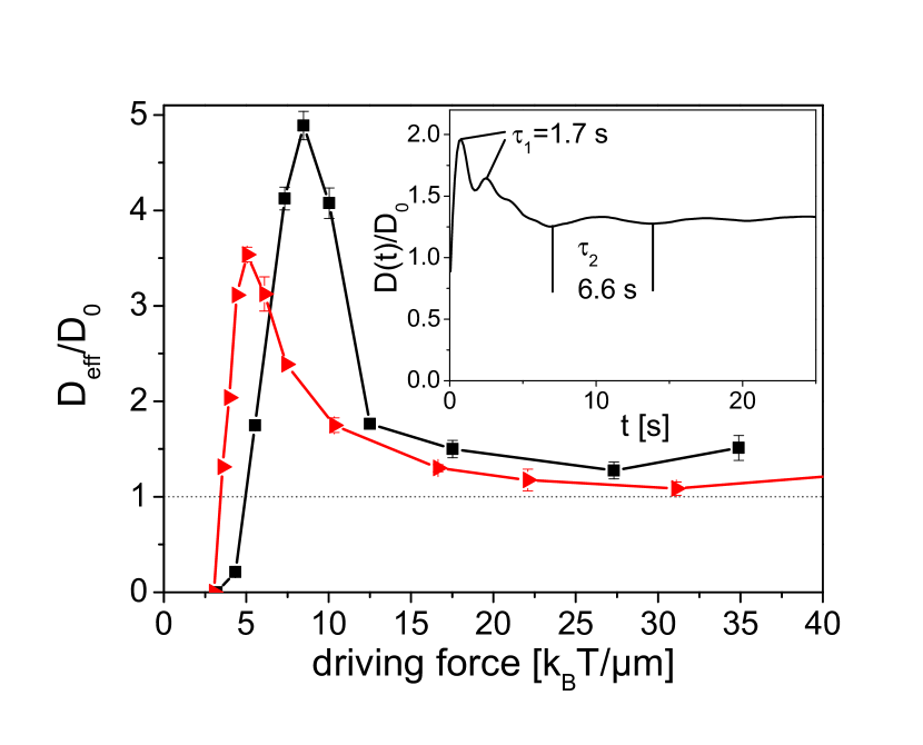
Figure 4: (color online) Normalized diffusion coefficient $D_{\mathrm{eff}}/D_{0}$ vs external driving force. The data was obtained for potential depths $V_{0}$ of $10.3$ ($\blacktriangleright$) and $14.4\,\mathrm{\mathit{k_{\mathrm{B}}T}}$ ($\blacksquare$). Inset: The function $D(t)$ in Eq. (10) versus time $t$ ($f\simeq 6.6\,\mathrm{kT/\mu m}$, $V_{0}\simeq 10.3\,\mathrm{\mathit{k_{\mathrm{B}}T}}$). After $15\,\mathrm{s}$ the long time limit is reached. The remaining small oscillations define the error in determining $D_{\mathrm{eff}}$.

$V_{0}$ [$\mathit{k_{\mathrm{B}}T}$]	$f_{c}[\,\mathrm{\mathit{k_{\mathrm{B}}T}/\mu m}]$		$D/D_{0}$
	exp.	theo.	exp.	theo.
14.4	8.5	7.3	4.9	3.1
10.3	5.1	5.2	3.5	2.5

Table 1: Comparison between experimentally determined and theoretically predicted position and height of the giant diffusion peak.

Fig. 4 shows the normalized effective diffusion coefficients for potential depths of $10.3$ and $14.4\,\mathit{k_{\mathrm{B}}T}$. Both curves show a peak clearly indicating the enhancement of thermal diffusion in tilted periodic potentials. With increasing potential strength we observe a shift of the $D_{\mathrm{eff}}(f)$ curve towards larger forces. The values of $f_{\mathrm{c}}$ and $D_{\mathrm{eff}}(f_{\mathrm{c}})$ sensitively depend on the shape of the potential and are theoretically predicted as $f_{\mathrm{c}}=2V_{0}/R$ and $D_{\mathrm{eff}}(f_{\mathrm{c}})=0.0696D_{0}(\frac{2}{3}V_{0}\pi^{3})^{(2/3)}$ rei01 .

A comparison with our data is shown in Tab. 1. While the predicted critical force $f_{\mathrm{c}}$ is in rather good agreement with the experimental data, the theoretical values systematically underestimate $D_{\mathrm{eff}}(f_{\mathrm{c}})/D_{0}$ by a factor of about $0.7$. The origin of this discrepancy is due to the aforementioned slight distortions along the toroidal trap which leads to local variations in the potential depth and thus affects the effective diffusion coefficient. Since at the same time the local shape of $V(x)$ is hardly affected by those distortions, the good agreement for the critical tilt can be explained.

Concluding perspective. – So far, we have demonstrated a novel method to reconstruct equilibrium potentials on the basis of the stationary probability distribution. In particular in one-dimensional NESS conditions, this quantity is easily determined experimentally, because the stationary current $j_{\mathrm{s}}$ is constant. When the method is extended to higher dimensions in the presence of nonconservative force fields $\mathbf{f}(\mathbf{r})$, in addition to the steady state probability $p_{\mathrm{s}}(\mathbf{r})$ the local mean velocity $\mathbf{v}_{\mathrm{s}}(\mathbf{r})=\mathbf{j}_{\mathrm{s}}(\mathbf{r})/p_{\mathrm{s}}(\mathbf{r})$ is required. Experimentally, this quantity is obtained by averaging the velocity of particles passing $\mathbf{r}$. Then the actual potential could be reconstructed through integration along open paths $C(\mathbf{r})$ starting at an arbitrary but fixed initial point and ending in $\mathbf{r}$, leading to

$$V(\mathbf{r})=-\mathit{k_{\mathrm{B}}T}\ln p_{\mathrm{s}}(\mathbf{r})\\ +\int_{C(\mathbf{r})}\left[\mathbf{f}(\mathbf{r}(s))-\gamma\mathbf{v}_{\mathrm{s}}(\mathbf{r}(s))\right]\cdot d\mathbf{r}(s).$$ (11)

In summary, we have demonstrated a flexible method to characterize potentials using the generalization of the inverted Boltzmann factor. In contrast to equilibrium measurements, this allows to characterize laser potentials up to depths of several hundredth or even thousandths of $\mathit{k_{\mathrm{B}}T}$. Based on the determination of the stationary state probability distribution $p_{\mathrm{s}}$, this technique is easily applicable to different situations, e.g. topographical potentials and does not require fast data acquisition techniques.

References

- (1) A. Mehta, M. Rief, J. Spudich, D. Smith, R. Simmons, Science 283, 1689 (1999).
- (2) M. Wang, H. Yin, R. Landick, J. Gelles, S. Block, Biophys. Jour. 72, 1335 (1997).
- (3) A. Ehrlicher, T. Betz, B. Stuhrmann, D. Koch, V. Milner, M. G. Raizen, J. Käs, Proc. Natl. Acad. Sci. U.S.A. 99, 16024 (2002).
- (4) K. Mangold, P. Leiderer, C. Bechinger, Phys. Rev. Lett. 90, 158302 (2003).
- (5) M. Brunner, C. Bechinger, Phys. Rev. Lett. 88, 248302 (2002).
- (6) M. McDonald, G. Spakling, K. Dholakia, Nature 426, 421 (2003).
- (7) K. Ladavac, D. Grier, Europhys. Lett. 70, 548 (2005).
- (8) A. Rohrbach, C. Tischner, D. Neumayer, E.-L. Florin, Rev. Sci. Instr. 75, 2197 (2004).
- (9) P. Poulin, V. Cabuil, D.A. Weitz, Phys. Rev. Lett. 79, 4862 (1997).
- (10) M. Skarabot, M. Ravnik, D. Babic, N. Osterman, I. Poberaj, S. Zumer, I. Musevic, Phys. Rev. E 73, 021705 (2006).
- (11) L. Faucheux, G. Stolovitzky, A. Libchaber, Phys. Rev. E 51, 5239 (1995).
- (12) P. Sheetz, Laser tweezers in cell biology, Academic Press, 1998.
- (13) L. Ghislain, N. Switz, W. Webb, Rev. Sci. Instr. 65, 2762 (1994).
- (14) T. Speck, U. Seifert, Europhys. Lett. 74, 391 (2006).
- (15) C. Lutz, M. Reichert, H. Stark, C. Bechinger, Europhys. Lett. 74, 719 (2006).
- (16) T. Tlusty, A. Meller, R. Bar-Ziv, Phys. Rev. Lett. 81, 1738, (1998).
- (17) P. Reimann, C. van den Broeck, H. Linke, P. Hänggi, J.M. Rubi, A. Perez-Madrid, Phys. Rev. Lett. 87, 10602 (2001), Phys. Rev. E 65, 031104, (2002).
- (18) S. Lee, D.G. Grier, Phys. Rev. Lett. 96, 190601, (2006).
- (19) S.A. Tatarkova, W. Sibbett, K. Dholakia, Phys. Rev. Lett. 91, 3, 038101, (2003).