Revisiting the one-dimensional diffusive contact process

Abstract

In this work we study the one-dimensional contact process with diffusion using two different approaches to research the critical properties of this model: the supercritical series expansions and finite-size exact solutions. With special emphasis we look to the multicritical point and its crossover exponent that characterizes the passage between DP and mean-field critical properties. This crossover occurs in the limit of infinite diffusion rate and our results pointed $\phi=4$ as the better estimate for the crossover exponent in agreement with computational simulations.

1 Introduction

In the last years there has been a growing interest in nonequilibrium phase transitions [1, 2]. The absence of a general theory nonequilibrium systems originates a great number of open problems, even in one-dimensional systems that, in the equilibrium regime, generally are exactly solvable. Usually, numerical simulations are a useful technique in the study of phase transitions and critical phenomena, and its power has been growing with the increasing capacity of the computers and the development of new simulational techniques. Non-equilibrium models are particularly suited for simulations. However, others approaches may be complementary in the study of these phenomena. Thus, it is interesting study the systems by other techniques. Among these alternative methods we can cite the series expansions [3], which in some cases lead to very precise estimates for the critical properties that characterize these transitions [3, 4] and the exact diagonalization of the time evolution operator in finite-size systems [5].

A special case of the non-equilibrium models are the ones that exhibit absorbing states [1], that is, states that may be reached in their dynamics, but transitions leaving them are forbidden. Since such models do not obey detailed balance, they are intrinsically out of equilibrium. The most studied system for this class of problems is the so called contact process (CP) model [6], a toy model for the spreading of an epidemic. This model displays a transition between an absorbing and an active state with critical exponents belonging to the directed percolation (DP) universality class [7]. In addition, the CP model is related to the Schlögl’s lattice model for autocatalytic reactions [8] and the Reggeon Field Theory [9].

Many variants of this model have been studied [10, 11, 12, 13], most of them belonging to DP class also. In fact, the robustness of this universality class is an evident characteristic of these models. Such robustness is explained by the conjecture that all models with phase transitions between active and absorbing states with a scalar order parameter, short range interactions and no conservation laws belong to this class [14].

One of these variants is the CP with diffusion [15], which exhibits a critical line instead of a critical point. This line begins at the critical point of the model without diffusion and ends in the infinite diffusion rate limit, where the critical properties of the system approaches those predicted by the mean-field approximation. For finite values of the diffusion rate, the critical behavior of this model is dominated by the DP universality class. This is not surprising, since the original dynamic includes an intrinsic diffusion process. On the other hand, the mean-field behavior in the limit of infinite diffusion may be understood considering that, since diffusion processes are dominating the evolution of the system in this limit, creation processes are effectively determined by the mean densities, as is supposed in the mean-field approximation. This change of behavior at the infinite diffusion rate limit, between the critical behavior of the DP class and the one predicted by the mean-field approximation, characterizes a crossover of the critical properties in the neighborhood of a multicritical point. As in the equilibrium case we may then write any density variable, in the neighborhood of a multicritical point, as the following scaling form [16]:

$$g(\alpha,D)=(\alpha_{c}-\alpha)^{\theta}F\left(\frac{D_{c}-D}{|\alpha_{c}-\alpha|^{\phi}}\right),$$ (1)

where $\alpha$ is a transition rate for annihilation of particles, $D$ is the diffusion rate, ranging between 0 and 1, $\theta$ is a critical exponent associated to the density variable $g$, corresponding to the value predicted by the mean-field approximation and $\phi$ is the crossover exponent. The scaling function $F(z)$ is singular at a point $z=z_{0}$ of its argument, such that the critical line, in the neighborhood of the multicritical point, corresponds to

$$(D_{c}-D)=z_{0}(\alpha_{c}-\alpha)^{\phi}.$$ (2)

One of the first studies of this problem was performed by Dickman and Jensen [15], who considered the model using supercritical series in $\alpha$ with the diffusion rate $D$ taken as a fixed parameter. Therefore, in their calculation series expansions are derived for fixed values of the diffusion rate $D$, and the analysis of this series leads, among other information, to the phase diagram of the model with diffusion. However, they found that the fluctuations of the estimates provided by d-log Padé approximants increase as the diffusion rate grows, so that the critical curve was obtained only up to $D\approx 0.8$. Since the crossover exponent $\phi$ characterizes the critical curve close to the infinite diffusion rate limit $D\to 1$ no precise estimate of the crossover exponent was possible. The disappointing performance of the Padé approximants as the multicritical point is approached is not surprising, since it is known tha one-variable series analysis techniques are not effective close to such points [16]. More recently [11], the model was simulated in a conservative ensemble. These simulations display smaller fluctuations in the estimates, making it possible to obtain the critical line up to values close to the multicritical point, furnishing the value $\phi=4.03(3)$ for the crossover exponent. This result is consistent with the lower bound $\phi\geq 1$ predicted by Katori in [17].

In the present work, we obtain estimates for the critical line, exponents $\beta$ and $z$ as well as the crossover exponent $\phi$ for the one-dimensional CP with diffusion. For this task we use two approaches: a two-variable supercritical series and exact solutions for finite-size one-dimensional lattices. The supercritical series is analyzed using a partial differential approximants (PDA s) [16, 18, 19]. This technique seems to be more appropriate for the analysis of a two-variable series with a multicritical behavior, as is shown by the results obtained for other models [12, 20]. This paper is organized as follows. In section II we present the model and the mean-field results, in section III we show the derivation of the supercritical series and in section IV the analysis of this series is presented. In section V we discuss the finite-size exact solution and their results for diffusive CP model. Finally, in section VI, the conclusions and final discussions of this work may be found.

2 Definition of the model and mean-field results

In a one-dimensional lattice each site can be empty or occupied by a particle, so that we will associate an occupation variable $\eta_{i}=0,1$ to the site $i$. The evolution of the system is governed by markovian local rules such that the particles are annihilated with rate $\alpha$ and created in empty sites with a transition rate $n/2$, where $n$ is the number of occupied nearest neighbors and $z$ is the total number of nearest neighbors. In addition to these rules that define the CP, we include a diffusive process, allowing the hopping of particles to empty nearest neighbor sites at the rate $\tilde{D}=D/(1-D)$. The configuration such that all sites are empty is an absorbing state. The passage from an active steady state, with a nonzero density of particles, to the absorbing state defines a transition line in the $(\alpha,D)$ plane as shown in figure 1.

A mean-field approach for this model can be obtained at several levels of approximation [1]. In the one-site level the role of the diffusion is irrelevant since it contributed equally to creation and annihilation of particles at a given site $i$. Already in the two-site level it is possible to determine the critical line by using as variables the parameters $\alpha$ and $D$. This line is described by the expression

$$(1-D)=\frac{\alpha(1-\alpha)}{3\alpha-\alpha-1}$$ (3)

and is very easy to show that in the neighborhood of the multicritical point, $(\alpha_{c}=1,D=1)$, the behavior of this curve is given by the scaling relation

$$(1-D)\sim(1-\alpha)^{\phi}$$ (4)

where $\phi=1$. On the three-site level an unitary crossover exponent also appears, as may be seen in figure 1.

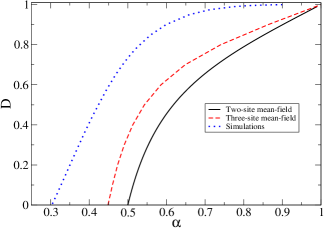
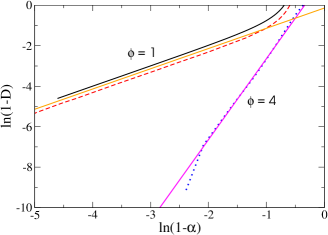
Figure 1: Top: phase diagram obtained using the two- and three-site mean-field approach and results of simulations [11]. Bottom: the log-log plot of the same quantity is plotted and compared to the result $\phi=1$ and $\phi=4$ for these approaches.

This result is in accordance with the lower bound, $\phi\geq 1$, determined by Katori [17]. Comparing the mean-field approximation with the simulational result [11], we observe that the first approach always overestimates the supercritical region of the models. Even in the higher diffusion region, the critical line obtained using mean-field does not coincide with the simulational result. Actually, this coincidence occurs only in the multicritical point.

In the next section we will derive the supercritical series in the variables $\lambda$ and $\tilde{D}$ to determine the value of this exponent and compare it with that obtained in [11, 15].

3 Derivation of the supercritical series for the model

We use the operator formalism proposed by Dickman and Jensen [4] in order to derive a supercritical series. To this end, we define the microscopic configuration of the lattice, $|\eta\rangle$, as the direct product of kets $|\eta\rangle=\bigotimes_{i}|\eta_{i}\rangle$, with the following orthonormality property, $\langle\eta|\eta^{\prime}\rangle=\prod_{i}\delta_{\eta_{i},\eta_{i}\prime}$. The particle creation and annihilation operators at site $i$ are defined as

$$A_{i}^{\dagger}|\eta_{i}\rangle = (1-\eta_{i})|\eta_{i}+1\rangle,$$

$$A_{i}|\eta_{i}\rangle = \eta_{i}|\eta_{i}-1\rangle.$$ (5)

In this formalism, the state of the system at time $t$ is

$$|\psi(t)\rangle=\sum_{\{\eta\}}p(\eta,t)|\eta\rangle,$$ (6)

where $p(\eta,t)$ is the probability of a configuration $\eta$ at time $t$. If we define the projection onto all possible states as $\langle\;|\equiv\sum_{\{\eta\}}\langle\eta|$ then the normalization of the state of the system may be expressed as $\langle\;|\psi\rangle=1$. In this notation, the master equation for the evolution of the state is:

$$\frac{d|\psi(t)\rangle}{dt}=S|\psi(t)\rangle.$$ (7)

The evolution operator $S$ may be expressed in terms of the creation and annihilation operators as $S=\mu R+V$ where

$$R = \tilde{D}\sum_{i}(1-A_{i-1}^{\dagger}A_{i})A_{i-1}A_{i}^{\dagger}+(1-A_{i+1}^{\dagger}A_{i})A_{i+1}A_{i}^{\dagger}+$$ (8)

$$+ \sum_{i}(A_{i}-A_{i}^{\dagger}A_{i}),$$

$$V = \sum_{i}(A_{i}^{\dagger}-A_{i}A_{i}^{\dagger})(A_{i-1}^{\dagger}A_{i-1}+A_{i+1}^{\dagger}A_{i+1}),$$ (9)

where $\mu\equiv 2\alpha$ and $\tilde{D}=D/\alpha$.

We notice that the operator $R$ diffuses $(01\to 10)$ or annihilates particles $(1\to 0)$, while the operator $V$ acts in the opposite way, generating particles $(0\to 1)$. It is convenient to join the diffusion with the annihilation process to avoid ambiguities in the truncation of the series at a certain order. For small values of the parameter $\mu$ the creation of particles is favored, and the decomposition above is convenient for a supercritical perturbation expansion. Using the equations (8) and (9) the action of each operator on a generical configuration $(\mathcal{C})$ is given by

$$R({\mathcal{C}}) = \tilde{D}\left[\sum_{i}({\mathcal{C}}^{\prime}_{i})+\sum_{j}({\mathcal{C}}^{\prime r}_{j})+\sum_{k}({\mathcal{C}}^{\prime l}_{k})\right]+$$ (10)

$$+ \sum_{t}({\mathcal{C}}^{\prime\prime}_{t})-[(r_{1}+2r_{2})+\tilde{D}+r]({\mathcal{C}}),$$

where the first sum is over $r_{1}$ sites with particles and one empty neighbor, the two next sums are over $r_{2}$ sites with particles and two empty neighbors and the last sum is over all sites occupied by a particle. Configuration $({\mathcal{C}}^{\prime}_{i})$ is obtained moving the particle at the site $i$ to the single empty neighbor site, $({\mathcal{C}}^{\prime(r,l)}_{i})$ is a configuration where the particle at the site $i$ moved to the empty neighbor at the right ($r$) or at the left ($l$) is replaced by a hole and one of the empty neighbors (at the right or left) is occupied. On the other hand, the action of operator $V$ is

$$V({\mathcal{C}})=\sum_{i}({\mathcal{C}}^{\prime\prime\prime}_{i})+2\sum_{j}({\mathcal{C}}^{\prime\prime\prime}_{j})-(q_{1}+2q_{2})({\mathcal{C}}),$$ (11)

where the first sum is over the $q_{1}$ empty sites with one occupied neighbor, the second sum is over the $q_{2}$ empty sites with two occupied neighbors. Configuration $({\mathcal{C}}_{i}^{\prime\prime\prime})$ is obtained occupying the site $i$ in configuration $(\mathcal{C})$.

To obtain a supercritical expansion for the ultimate survival probability of particles, we start by remembering that in order to access the long-time behavior of a quantity, it is useful to consider its Laplace transform,

$$|\tilde{\psi}(s)\rangle=\int_{0}^{\infty}e^{-st}|\psi(t)\rangle.$$ (12)

Inserting the formal solution $|\psi(t)\rangle=e^{St}|\psi(0)\rangle$ of the master equation (7) we find

$$|\tilde{\psi}(s)\rangle=(s-S)^{-1}|\psi(0)\rangle.$$ (13)

The stationary state $|\psi(\infty)\rangle\equiv\lim_{t\to\infty}|\psi(t)\rangle$ may then be found by means of the relation

$$|\psi(\infty)\rangle=\lim_{s\to 0}s|\tilde{\psi}(s)\rangle.$$ (14)

A perturbative expansion may be obtained by assuming that $|\tilde{\psi}(s)\rangle$ can be expressed in powers of $\mu$ and using (13),

$$|\tilde{\psi}(s)\rangle=|\tilde{\psi}_{0}\rangle+\mu|\tilde{\psi}_{1}\rangle+\mu^{2}|\tilde{\psi}_{2}\rangle+\cdots=(s-V-\mu R)^{-1}|\psi(0)\rangle.$$ (15)

Since

$$(s-V-\mu R)^{-1}=(s-V)^{-1}\left[1+\mu(s-V)^{-1}R+\mu^{2}(s-V)^{-2}R^{2}+\cdots\right],$$ (16)

we arrive at

$$|\tilde{\psi}_{0}\rangle=(s-V)^{-1}|\psi(0)\rangle$$ (17)

and

$$|\tilde{\psi}_{n}\rangle=(s-V)^{-1}R|\tilde{\psi}_{n-1}\rangle,$$ (18)

for $n\geq 1$. The action of the operator $(s-V)^{-1}$ on an arbitrary configuration $({\mathcal{C}})$ may be found by noticing that

$$(s-V)^{-1}({\mathcal{C}})=s^{-1}\left\{({\mathcal{C}})+(s-V)^{-1}V({\mathcal{C}})\right\},$$ (19)

and using the expression 11 for the action of the operator $V$, we get

$$(s-V)^{-1}({\mathcal{C}})=s_{q}\left\{({\mathcal{C}})+(s-V)^{-1}\left[\sum_{i}({\mathcal{C}}^{\prime\prime\prime}_{i})+2\sum_{j}({\mathcal{C}}^{\prime\prime\prime}_{j})\right]\right\},$$ (20)

where the first sum is over the $q_{1}$ empty sites and one occupied neighbor, the second sum is over the $q_{2}$ empty sites and two occupied neighbors, and we define $s_{q}\equiv 1/(s+q_{1}+2q_{2})$.

It is convenient to adopt as the initial configuration a translational invariant one with a single particle (periodic boundary conditions are used). Now, looking at the recursive expression (20), we may notice that the operator $(s-V)^{-1}$ acting on any configuration generates an infinite set of configurations, and thus we are unable to calculate $|\tilde{\psi}\rangle$ in a closed form. However, it is possible calculate the extinction probability $\tilde{p}(s)$, which corresponds to the coefficient of the vacuum state $|0\rangle$. As happens also for models [4, 3] related to the CP, configurations with more than $j$ particles only contribute at orders higher than $j$, and since we are interested in the ultimate survival probability for particles $P_{\infty}=1-\lim_{s\to 0}s\tilde{p}(s)$, $s_{q}$ may be replaced by $1/q$ in equation (20). An illustration of this procedure may be found in a previous calculation [12].

The algebraic operations described above is performed by a simple algorithm which allow us to calculate 24 terms with a processing time to about 2 hours. Actually, the limiting factor in this operation is the memory required. In this way we define the coefficients $b_{i,j}$ for the ultimate survival probability as:

$$P_{\infty}=1-\frac{1}{2}\mu-\frac{1}{4}\mu^{2}-\sum_{i=3}^{24}\sum_{j=0}^{i-2}b_{i,j}\mu^{i}\tilde{D}^{j},$$ (21)

and they are listed in Table 1.

Table 1: Coefficients for the series expansion for ultimate survival probability corresponding to the CP model with diffusion. The indexes refer them to the equation (21).

i	j	$b_{i,j}$	i	j	$b_{i,j}$
3	0	0.25000000000000000000$\times 10^{0}$		6	0.10567643059624561630$\times 10^{2}$
	1	-0.25000000000000000000$\times 10^{0}$		7	0.34998474121093847700$\times 10^{1}$
4	0	0.28125000000000000000$\times 10^{0}$		8	0.12568359375000000000$\times 10^{2}$
	1	-0.37500000000000000000$\times 10^{0}$	11	0	0.24775957118666096513$\times 10^{1}$
	2	0.37500000000000000000$\times 10^{0}$		1	-0.71703082845177412707$\times 10^{1}$
5	0	0.34375000000000000000$\times 10^{0}$		2	0.12429764028158224676$\times 10^{2}$
	1	-0.50781250000000000000$\times 10^{0}$		3	-0.16676337106809967281$\times 10^{2}$
	2	0.57812500000000000000$\times 10^{0}$		4	0.19435605471721252968$\times 10^{2}$
	3	-0.62500000000000000000$\times 10^{0}$		5	-0.15230894658300556443$\times 10^{2}$
6	0	0.44726562500000000000$\times 10^{0}$		6	0.13923689787279895924$\times 10^{2}$
	1	-0.76220703125000000000$\times 10^{0}$		7	-0.24910518081099844778$\times 10^{2}$
	2	0.85058593750000000000$\times 10^{0}$		8	-0.13853664539478481643$\times 10^{2}$
	3	-0.83984375000000000000$\times 10^{0}$		9	-0.23740234375000000000$\times 10^{2}$
	4	0.10937500000000000000$\times 10^{0}$
7	0	0.60223388671874955591$\times 10^{0}$	12	0	0.36488812342264926869$\times 10^{1}$
	1	-0.11734619140625004441$\times 10^{1}$		1	-0.11443929729648042226$\times 10^{2}$
	2	0.15190429687499997780$\times 10^{1}$		2	0.21418735868689896762$\times 10^{2}$
	3	-0.14140624999999984457$\times 10^{1}$		3	-0.29831307350977681381$\times 10^{2}$
	4	0.10878906249999982236$\times 10^{1}$		4	0.34272964785342651339$\times 10^{2}$
	5	-0.19687500000000000000$\times 10^{1}$		5	-0.40398672142671166796$\times 10^{2}$
8	0	0.83485031127929687500$\times 10^{0}$		6	0.27855684964608855125$\times 10^{2}$
	1	-0.18110389709472716202$\times 10^{1}$		7	-0.13595902518316915319$\times 10^{2}$
	2	0.25234603881835981909$\times 10^{1}$		8	0.60935236387946176251$\times 10^{2}$
	3	-0.29291381835937464473$\times 10^{1}$		9	0.40270442479922508028$\times 10^{2}$
	4	0.24864501953125062172$\times 10^{1}$		10	0.45106445312500000000$\times 10^{2}$
	5	-0.10754394531250017764$\times 10^{1}$	13	0	0.54293656084851154020$\times 10^{1}$
	6	0.36093750000000000000$\times 10^{1}$		1	-0.18322144692814863021$\times 10^{2}$
9	0	0.11814667913648828623$\times 10^{1}$		2	0.36259195896082665911$\times 10^{2}$
	1	-0.28569926950666579835$\times 10^{1}$		3	-0.54866931326313050477$\times 10^{2}$
	2	0.42781094621729156557$\times 10^{1}$		4	0.67130818799164941879$\times 10^{2}$
	3	-0.48761836864330092567$\times 10^{1}$		5	-0.64293858561553619779$\times 10^{2}$
	4	0.54410674483687788694$\times 10^{1}$		6	0.81638245065997452343$\times 10^{2}$
	5	-0.48496839735243062464$\times 10^{1}$		7	-0.59206203158103356543$\times 10^{2}$
	6	0.11848958333333414750$\times 10^{0}$		8	-0.11386872839957611347$\times 10^{2}$
	7	-0.67031250000000000000$\times 10^{1}$		9	-0.15017302299755911577$\times 10^{3}$
10	0	0.16988672076919952847$\times 10^{1}$		10	-0.10358591484729181786$\times 10^{3}$
	1	-0.45030223008843064392$\times 10^{1}$		11	-0.8611230468750000000$\times 10^{2}$
	2	0.73700355965291270977$\times 10^{1}$	14	0	0.8132542219307161701600$\times 10^{1}$
	3	-0.92486491500105252328$\times 10^{1}$		1	-0.29467694610727896531$\times 10^{2}$
	4	0.87502182305104447835$\times 10^{1}$		2	0.62075441392908530247$\times 10^{2}$
	5	-0.93882905701060082038$\times 10^{1}$		3	-0.96520364146752442025$\times 10^{2}$

i	j	$b_{i,j}$	i	j	$b_{i,j}$
14	4	0.12740413805065173847$\times 10^{3}$		3	-0.55737662171810006839$\times 10^{3}$
	5	-0.14872799806680012580$\times 10^{3}$		4	0.80584299514354984240$\times 10^{3}$
	6	0.11055259565281477308$\times 10^{3}$		5	-0.10663609887965685630$\times 10^{4}$
	7	-0.15322889380857196784$\times 10^{3}$		6	0.12359653482806177180$\times 10^{4}$
	8	0.15125687744198603468$\times 10^{3}$		7	-0.86967640846259655518$\times 10^{3}$
	9	0.12100775973170790678$\times 10^{3}$		8	0.16397080915531578285$\times 10^{4}$
	10	0.36717258144235222517$\times 10^{3}$		9	-0.72176857313912660175$\times 10^{3}$
	11	0.24952145042880511028$\times 10^{3}$		10	-0.39467789553376610456$\times 10^{3}$
	12	0.16504858398437500000$\times 10^{3}$		11	-0.37241724510229601037$\times 10^{4}$
15	0	0.12275012836144505002$\times 10^{2}$		12	-0.43433579993156563432$\times 10^{4}$
	1	-0.47363165128788978109$\times 10^{2}$		13	-0.49111545112523144780$\times 10^{4}$
	2	0.10546586796137503939$\times 10^{3}$		14	-0.28643360597728060384$\times 10^{4}$
	3	-0.1762739398241103288$\times 10^{3}$		15	-0.11834527587890625000$\times 10^{4}$
	4	0.23298609118631188153$\times 10^{3}$	18	0	0.435207828742268674200$\times 10^{2}$
	5	-0.27071715385838172097$\times 10^{3}$		1	-0.20009555228747112210$\times 10^{3}$
	6	0.33267266081610591755$\times 10^{3}$		2	0.51666085550451919062$\times 10^{3}$
	7	-0.18014432368848466126$\times 10^{3}$		3	-0.98221829678260564833$\times 10^{3}$
	8	0.24323790718884771422$\times 10^{3}$		4	0.15468813789798582548$\times 10^{4}$
	9	-0.43351480900655008099$\times 10^{3}$		5	-0.19452358996876919264$\times 10^{4}$
	10	-0.48110863117407200207$\times 10^{3}$		6	0.23142581042234874076$\times 10^{4}$
	11	-0.88513499744041246231$\times 10^{3}$		7	-0.29269143532222028625$\times 10^{4}$
	12	-0.57707323452079549497$\times 10^{3}$		8	0.11929249112512670763$\times 10^{4}$
	13	-0.31740112304687500000$\times 10^{3}$		9	-0.33469260525748682085$\times 10^{4}$
16	0	0.18620961415130427241$\times 10^{2}$		10	0.22662397929431922421$\times 10^{4}$
	1	-0.76547748518027589171$\times 10^{2}$		11	0.33534053058169365613$\times 10^{4}$
	2	0.17936794520034777634$\times 10^{3}$		12	0.10497352179518215053$\times 10^{5}$
	3	-0.30967915791812674797$\times 10^{3}$		13	0.11603782689493993530$\times 10^{5}$
	4	0.45127497217248452444$\times 10^{3}$		14	0.11326231062527707763$\times 10^{5}$
	5	-0.53698491310493750461$\times 10^{3}$		15	0.62269615466431168898$\times 10^{4}$
	6	0.51912309945306844838$\times 10^{3}$		16	0.22929397201538085938$\times 10^{4}$
	7	-0.74776029427868388666$\times 10^{3}$	19	0	0.66930218067969633466$\times 10^{2}$
	8	0.31390176074091152714$\times 10^{3}$		1	-0.32354897975245813768$\times 10^{3}$
	9	-0.23066668763466492464$\times 10^{3}$		2	0.88042629554806353553$\times 10^{3}$
	10	0.12806582574012411442$\times 10^{4}$		3	-0.17413898514485581472$\times 10^{4}$
	11	0.15251186818533849419$\times 10^{4}$		4	0.27574673463423659996$\times 10^{4}$
	12	0.21006816788719602300$\times 10^{4}$		5	-0.39760107863198809355$\times 10^{4}$
	13	0.12983815231244370807$\times 10^{4}$		6	0.45478180647223589403$\times 10^{4}$
	14	0.61213073730468750000$\times 10^{3}$		7	-0.44829538123020120111$\times 10^{4}$
17	0	0.28405733950686048672$\times 10^{2}$		8	0.71439950475520599866$\times 10^{4}$
	1	-0.12342415559750365617$\times 10^{3}$		9	-0.11433220550468702186$\times 10^{4}$
	2	0.30541526863109334045$\times 10^{3}$		10	0.58699584417021997069$\times 10^{4}$

i	j	$b_{i,j}$	i	j	$b_{i,j}$
19	11	-0.80007309950477119855$\times 10^{4}$		15	-0.19550932821134978440$\times 10^{6}$
	12	-0.13849586891129882133$\times 10^{5}$		16	-0.17865808405461237999$\times 10^{6}$
	13	-0.28630836746692133602$\times 10^{5}$		17	-0.13001245697926016874$\times 10^{6}$
	14	-0.29699369329023520550$\times 10^{5}$		18	-0.60334798749708410469$\times 10^{5}$
	15	-0.25808082841629722679$\times 10^{5}$		19	-0.16853935146331787109$\times 10^{5}$
	16	-0.13385541065918856475$\times 10^{5}$	22	0	0.24876519640902955643$\times 10^{3}$
	17	-0.44510006332397460938$\times 10^{4}$		1	-0.13849806980532957823$\times 10^{4}$
20	0	0.10337399908883011790$\times 10^{3}$		2	0.42491525612070690840$\times 10^{4}$
	1	-0.52548922262251915072$\times 10^{3}$		3	-0.95509490156905540061$\times 10^{4}$
	2	0.14837268484319015442$\times 10^{4}$		4	0.17072122607398174296$\times 10^{5}$
	3	-0.30794482965317188246$\times 10^{4}$		5	-0.25259991312968326383$\times 10^{5}$
	4	0.51825134723219762236$\times 10^{4}$		6	0.36959825267281092238$\times 10^{5}$
	5	-0.70384028435684167562$\times 10^{4}$		7	-0.39724946702482979163$\times 10^{5}$
	6	0.95392163017937873519$\times 10^{4}$		8	0.41082488201681495411$\times 10^{5}$
	7	-0.10775090683332531626$\times 10^{5}$		9	-0.69996295461125846487$\times 10^{5}$
	8	0.72306238600702890835$\times 10^{4}$		10	-0.47433844045513687888$\times 10^{4}$
	9	-0.17556031650766155508$\times 10^{5}$		11	-0.94472082453477501986$\times 10^{5}$
	10	0.45576565336850308086$\times 10^{3}$		12	0.18231631734823597071$\times 10^{5}$
	11	-0.68853229355527937514$\times 10^{4}$		13	0.74507403911089320900$\times 10^{5}$
	12	0.27725591978402942914$\times 10^{5}$		14	0.28127919612702319864$\times 10^{6}$
	13	0.46620453043310422800$\times 10^{5}$		15	0.40344708716105029453$\times 10^{6}$
	14	0.75787894589888033806$\times 10^{5}$		16	0.49346542769156675786$\times 10^{6}$
	15	0.73699439769879478263$\times 10^{5}$		17	0.42523410507562680868$\times 10^{6}$
	16	0.58191226154708187096$\times 10^{5}$		18	0.28817317888963740552$\times 10^{6}$
	17	0.28519783989193914749$\times 10^{5}$		19	0.12690253004534545471$\times 10^{6}$
	18	0.86547234535217285156$\times 10^{4}$		20	0.32865173535346984863$\times 10^{5}$
21	0	0.15998830271612598608$\times 10^{3}$	23	0	0.38696067609131841891$\times 10^{3}$
	1	-0.85206464313625656359$\times 10^{3}$		1	-0.22521288931067451813$\times 10^{4}$
	2	0.25270411365871177622$\times 10^{4}$		2	0.72239403631839231821$\times 10^{4}$
	3	-0.53883333002320678133$\times 10^{4}$		3	-0.16540644823073282168$\times 10^{5}$
	4	0.93069165541648508224$\times 10^{4}$		4	0.30965978110985601234$\times 10^{5}$
	5	-0.14256926805592749588$\times 10^{5}$		5	-0.49715203648917136888$\times 10^{5}$
	6	0.16894039347875652311$\times 10^{5}$		6	0.63140021723358484451$\times 10^{5}$
	7	-0.21057424914324066776$\times 10^{5}$		7	-0.90160716109902248718$\times 10^{5}$
	8	0.2676311383571557235$\times 10^{5}$		8	0.96095356087432839558$\times 10^{5}$
	9	-0.76173492536429366737$\times 10^{4}$		9	-0.63690648044614848914$\times 10^{5}$
	10	0.42006937485571783327$\times 10^{5}$		10	0.18830794813510467065$\times 10^{6}$
	11	-0.12698208721358355433$\times 10^{4}$		11	0.57163083968398816069$\times 10^{5}$
	12	-0.53474107987358220271$\times 10^{4}$		12	0.19078924010583921336$\times 10^{6}$
	13	-0.90835383726464555366$\times 10^{5}$		13	-0.11462564856718564988$\times 10^{6}$
	14	-0.14158471202173284837$\times 10^{6}$		14	-0.34295621170633088332$\times 10^{6}$

i	j	$b_{i,j}$
23	15	-0.83015840201854216866$\times 10^{6}$
	16	-0.11002212525564364623$\times 10^{7}$
	17	-0.12227985275158903096$\times 10^{7}$
	18	-0.99733247054306510836$\times 10^{6}$
	19	-0.63431234698974736966$\times 10^{6}$
	20	-0.26563714369463571347$\times 10^{6}$
	21	-0.64165338807344436646$\times 10^{5}$
24	0	0.60509199550873199769$\times 10^{3}$
	1	-0.36606232348859748527$\times 10^{4}$
	2	0.12139375556095224965$\times 10^{5}$
	3	-0.29330923818458009919$\times 10^{5}$
	4	0.55510496259245075635$\times 10^{5}$
	5	-0.89523794399456470273$\times 10^{5}$
	6	0.13690056986421268084$\times 10^{6}$
	7	-0.14950913041347730905$\times 10^{6}$
	8	0.20276027262469305424$\times 10^{6}$
	9	-0.24868958310934680048$\times 10^{6}$
	10	0.44658906685524416389$\times 10^{5}$
	11	-0.50473239786133670714$\times 10^{6}$
	12	-0.20583143731838543317$\times 10^{6}$
	13	-0.31319042987920023734$\times 10^{6}$
	14	0.51903724071582528995$\times 10^{6}$
	15	0.12406518345377091318$\times 10^{7}$
	16	0.23558257104359627701$\times 10^{7}$
	17	0.29049027840298512019$\times 10^{7}$
	18	0.29832956761808455922$\times 10^{7}$
	19	0.23110049545479607768$\times 10^{7}$
	20	0.13877345160856433213$\times 10^{7}$
	21	0.55381177327087428421$\times 10^{6}$
	22	0.12541407130479812622$\times 10^{6}$

4 Analysis of the series

To obtain estimates of the critical properties, specially the critical line, from the supercritical series for the ultimate survival probability as given by the equation (21), we initially use d-log Padé approximants. These approximants are defined as ratios of two polynomials

$$F_{LM}(\lambda)=\frac{P_{L}(\lambda)}{Q_{M}(\lambda)}=\frac{\sum_{i=0}^{L}p_{i}\lambda^{i}}{1+\sum_{j=1}^{M}q_{j}\lambda^{j}}=f(\lambda).$$ (22)

In our case the function $f(\lambda)$ represents the series for $\frac{d}{d\lambda}\ln P_{\infty}(\lambda)$. As $f(\lambda)$ is a function of one variable, we fix the value of $\tilde{D}$ to calculate these approximants. For a fixed value of $\tilde{D}$ one pole of the approximant $F$ will correspond to the critical point while the associated residue will be the critical exponent $\beta$. We calculate approximants with $L+M\leq 24$, restricting our calculation to diagonal or close to diagonal approximants, which usually display a better convergence. Thus $L=M+\xi$, where $\xi=0,\pm 1$ and with $D=\tilde{D}/(1+\tilde{D})$ ranging between 0 and 0.8. Examples of estimates for the critical values of $\mu$ obtained from these approximants is given in Table 2 for different values of the diffusion.

D	L	M	$\mu_{c}$
0	10	10	0.60645
	11	11	0.60646
0.1	10	10	0.62267
	11	11	0.62266
0.7	10	10	0.85353
	11	11	0.84513
0.8	10	10	0.96256
	11	11	0.94246

Table 2: Estimates for critical points obtained by d-log Padé approximants. Note that as the value of $D=\tilde{D}/(1+\tilde{D})$ grows the dispersion in the value estimates also increases.

For each value of the diffusion rate, we calculate about eight approximants, obtaining the estimate of $\mu_{c}$ associated to diffusion as an arithmetic average of results furnished by these set of approximants and error bar associated to it corresponds to standard deviation of the estimates. From this we obtain the phase diagram shown in the figure 2. With the purpose of comparison with the results coming from the conservative simulations [11] we use the variables $\alpha\equiv\mu/2$ and $D_{eff}=\alpha\tilde{D}/(1+\alpha\tilde{D})$. We also calculate the $\beta$ exponent associated to the order parameter for differents values of $D$ exhibited in the figure 3. Similar to what happens with the critical point a growing fluctuation for high diffusion rate values is visible.

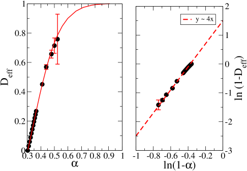
Figure 2: At left panel we have the phase diagram obtained by simulations (solid curve) and through Pades approximants for the supercritical series (circles). At right the log-log plot of the same quantity is plotted showing that value of the crossover exponent $\phi=4$ is a reasonable estimate for this data.

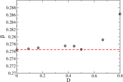
Figure 3: Estimates of the exponent $\beta$ for different diffusion rates. The dashed line indicates the DP value for this exponent.

Turning back to the discussion about the critical line, we see that for higher values of the diffusion the dispersion increases, and estimates with larger error bars are found. Nevertheless, the exponent $\phi=4$ seems to describe well the calculated points of the critical line. However, this result would be different if we used approximants to series closer to the infinite diffusion rate limit. This error in the approximants for high values of the diffusion rate is attributed to the alternated sign of the series terms [15]. Another explanation would come from the fact that in the neighborhood of a multicritical point the reduction of a two-variable series to one variable leads to very poor estimates of the critical properties [12] close to a multicritical point. To overcome this problem we analyze the series using Partial Differential Approximants (PDA’s) [16], that generalize the d-log Padé approximants for a two-variable series. These approximants are defined by the following equation

$$P_{\mathbf{L}}(x,y)F(x,y)=Q_{\mathbf{M}}(x,y)\frac{\partial F(x,y)}{\partial x}+R_{\mathbf{N}}(x,y)\frac{\partial F(x,y)}{\partial y},$$ (23)

where $P$, $Q$, and $R$ are polynomials in the variables $x$ and $y$ with the set of nonzero coefficients ${\mathbf{L}}$, ${\mathbf{M}}$, and ${\mathbf{N}}$, respectively. The coefficients of the polynomials are obtained by substitution of the series expansion of the quantity which is going to be analyzed

$$f(x,y)=\sum_{k,k^{\prime}=0}f(k,k^{\prime})x^{k}y^{k^{\prime}}$$ (24)

into equation (23) and requiring the equality to hold for a set of indexes defined as ${\mathbf{K}}$. This procedure leads to a system of linear equations for the coefficients of the polynomials, and since the coefficients $f_{k,k^{\prime}}$ of the series are known for a finite set of indexes this places an upper limit to the number of coefficients in the polynomials. Since the number of equations has to match the number of unknown coefficients, the numbers of elements in each set must satisfy $K=L+M+N-1$ (one coefficient is fixed arbitrarily). An additional issue, which is not present in the one-variable case, is the symmetry of the polynomials. Two frequently used options are the triangular and the rectangular arrays of coefficients. The choice of these symmetries may be related to the symmetry of the series itself [18]. In our case, the series presents a triangular symmetry when express in terms of the variables $x=\alpha$ and $y=\alpha\tilde{D}/(1+\alpha\tilde{D})$.

It is possible to show [18] that we can determine the multicritical properties using the equation 23 and the hypothesis of that in the neighborhood of the multicritical point, the function $f$ obeys the following scaling form

$$f(x,y)\approx|\Delta\widetilde{x}|^{-\nu}Z\left(\frac{|\Delta\widetilde{y}|}{|\Delta\widetilde{x}|^{\phi}}\right),$$ (25)

where

$$\Delta\widetilde{x}=(x-x_{c})-(y-y_{c})/e_{2},$$ (26)

and

$$\Delta\widetilde{y}=(y-y_{c})-e_{1}(x-x_{c}).$$ (27)

Here $\nu$ is the critical exponent of the quantity described by $f$ when $\Delta\widetilde{y}=0$, $e_{1}$ and $e_{2}$ are the scaling slopes [16] and $\phi$ is the crossover exponent.

On the other side, our calculation was successful when we use the method of the characteristics to integrate equation (23). This is made by introducing a timelike variable $\tau$, so that a family of curves is obtained in the plane $(x(\tau),y(\tau))$ (the characteristics). Such curves obey to the equations

$$\frac{dx}{d\tau} = Q_{M}(x(\tau),y(\tau)),$$

$$\frac{dy}{d\tau} = R_{N}(x(\tau),y(\tau)).$$ (28)

It is possible to show that integrating the equations (28) from a specific point of the critical line, the resulting characteristic is equivalent to the the critical line. In figure 4 we show a comparison between a characteristic curve and the simulational result [11]. The number of elements in the sets of the calculated approximants was varying as follows: $K=55-190$, $M=N=20-53$ and $L=15-54$.

In each of these curves, we calculate his inclination in the neighborhood of the multicritical point, determining a value for the exponent $\phi$ and the mean value for this exponent results as $\phi=4.02\pm 0.13$, consistent with simulations in the particle conserving ensemble [11].

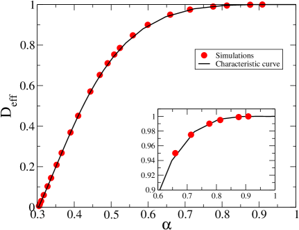
Figure 4: Comparison between a characteristic curve (solid line) and a numerical simulation result (circles). The coincidence is evident, including the region close to the infinite diffusion limit (inset).

Using all the characteristic curves calculated we derive an ‘average curve’, calculating for each value of $\alpha$ on arithmetic average for $D_{eff}$. This curve is shown in the figure 5 jointly with the result originating from the simulation and with the scaling form $(1-D_{eff})\sim(1-\alpha)^{4}$. In the same figure we see that the exponent $\phi=4$ is well fitted to the results of simulation and of the PDA’s. This scaling form is based on the argument of the scaling function $Z$ presented in the equation (25), where $\phi=4$ and $z_{0}$ is a parameter properly chosen. We remark that this scaling form coincides with the characteristic curve and with the simulation even in the weak diffusion regime. This is somewhat surprising since its validity would be expected only in the neighborhood of the multicritical point.

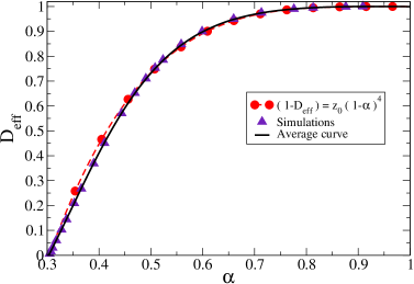
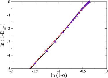
Figure 5: Comparison between a characteristic ‘average curve’ (solid line), the numerical simulation results (triangles) and the curve obtained from the scaling form $(1-D_{eff})\sim(1-\alpha)^{4}$(circles). At the right panel we see that $\phi=4$ seems to be a good estimative for the crossover exponent.

Unfortunately, even using the algorithm proposed by Styer [18] we were not able to obtain precise estimates for the crossover exponent $\phi$ from the scaling form shown in equation (25). However, integrating a set of approximants, we could determine the characteristic curves whose initial point is coincident with the critical point of the CP without diffusion of particles. These curves are estimates for the critical line of the CP model with diffusion going beyond the values achieved in [15] and [11] and corroborating the initial result of this last reference in that $\phi\approx 4$.

5 Exact solution for finite systems

An interesting approach to study stochastic systems is the exact solution of models with increasing numbers of sites L followed by extrapolations to the thermodynamic limit [5]. This is accomplished by considering operator $S$ and its eigenvalues. For process governed by the master equation vanishing eigenvalues,$\mu_{0}=0$, of the evolution operator correspond to stationary states of the system. For finite systems with absorbing states, only these states are stationary, and no active stationary state is found. To study the transition between an active and a stationary state, we may consider the behavior of the eigenvalue with the second smallest absolute value $\Gamma=|\mu_{1}|$ of the operator. This eigenvalue is related to the quasi-stationary state [21] and will eventually become degenerate with $\mu_{0}$ in the thermodynamic limit, originating the phase transition.

In a one-dimensional lattice with $L$ sites, we construct a set of configurations that works as basis of the operator. Using periodic boundary conditions some of these configurations will be related for a symmetry $C_{L}$ over cyclic rotations. These symmetries reduces the number of the independent vectors of the basis.

On the other hand, a scaling behavior for $\Gamma$, with $D$ held fixed, is given by the expression

$$\Gamma=L^{-z}f(\Delta L^{1/\nu_{\perp}}),$$ (29)

where $\Delta=|\alpha_{c}-\alpha|$. Defining the quantity

$$Y_{L}(\alpha,D)=\frac{\ln[\Gamma(\alpha,D;L+1)/\Gamma(\alpha,D;L-1)]}{\ln[(L+1)/(L-1)]},$$ (30)

we may estimate the critical point $\alpha_{c}(L)$ finding the intersection of the curves $Y_{L}$ and $Y_{L+1}$ [5]. This procedure resembles the phenomenological renormalization group [22]. The sequence $\alpha_{c}(L)$ of estimates for a given value of $D$, with $L$ ranging between 4 and 14, was extrapolated to the thermodynamic limit, producing a critical line shown in the figure 6. Although in the higher diffusion region the coincidence between the two lines, shown in the figure, reduces there seems to be no doubt that $\phi=4$ is a good estimate for the crossover exponent. Actually, the estimative for this exponent using the exact diagonalization approach is $\phi=3.87\pm 0.17$. Probably for high diffusions is necessary to study larger lattices to determine more precise results for the critical point as well as its exponent. The exponent $z$ is shown as function of the diffusion rate in the figure 7. For smaller diffusion rate, the exponent value coincide with that predicted by the DP universality class. However, for $D>0.2$ occurs a growing of this estimative and a simple quadratic extrapolation gives $z=1.93$, near to multicritical point, which is in reasonable agreement with mean-field value for this exponent, $z=2$.

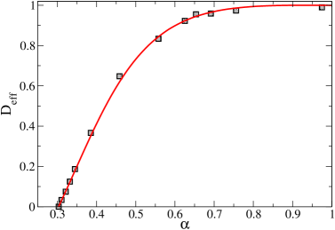
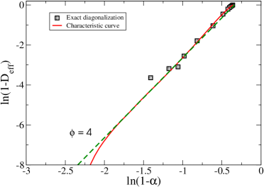
Figure 6: Comparison between a ’average’ characteristic curve (solid line) and the exact diagonalization result (squares). At the right panel we see that $\phi=4$ is a good estimative for the crossover exponent.

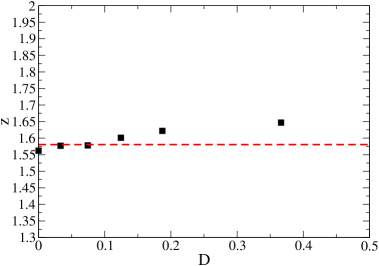
Figure 7: Estimative for the $z$ exponent calculated by some values of the diffusion rate. The dashed line indicates the DP value.

6 Conclusion

We study the difussive contact process in one-dimension analyzing its critical properties. A special attention is devoted for the determination of the crossover between a classical mean-field behavior in the infinite diffusion limit and DP universality class presents when the diffusion rate is finite. To accomplish this task we use supercritical pertubative series and exact solutions for finite-size lattices.

Calculating a supercritical series for the ultimate survival probability and analyzing it using PDA’s we obtain estimates for the critical line of the CP model with diffusion. The critical line was derived through the integration of the equation (23) by the method of the characteristics. Direct results for the value of the crossover exponent using the scaling form 25 using Styer’s algorithm [18] we were not be able to be obtain with an acceptable precision. However the method of the characteristics permitted us to calculate the critical line and, consequently, the value for the crossover exponent $\phi$. Our result, $\phi=4.02\pm 0.13$ is in agreement with that derived in [11] and explores a region of diffusion very close to the multicritical point.

The technique of the two-variable supercritical series associated with PDA analysis was shown to be accurate enough to determine the critical properties in similar models [12]. Therefore, we believe that a natural extension for this work is analyze related models that apparently possess non-trivial multicritical points. This seems to be the cases of the pair-creation and triplet-creation models with diffusion, also studied in [11]. This research is already in course.

Finally, the results provided by the exact diagonalization of the time evolution operator are according to simulational data as well as that ones obtained by the series analysis. Actually, in higher diffusion region, a greater fluctuation take place, suggesting that this system must be studied in larger sizes. Nevertheless, the critical curve indicates that $\phi\approx 4$ is a good estimate for the crossover exponent.

References

References

- [1] J. Marro and R. Dickman, Nonequilibrium Phase Transitions in Lattice Models (Cambridge University Press, Cambridge, 1999)
- [2] Nonequilibrium Statistical Mechanics in One Dimension edited by V. Privman, (Cambridge University Press, Cambridge, 1997)
- [3] I. Jensen and R. Dickman, J. Stat. Phys. 71, 89 (1993).
- [4] R. Dickman and I. Jensen, Phys. Rev. Lett. 67,2391 (1991).
- [5] E. Carlon, M. Henkel and U. Schollw ck, Eur. Phys. J. B 12,99 (1999).
- [6] T.E. Harris, Ann. Probab. 2, 969 (1974).
- [7] I. Jensen, J. Phys. A , ().
- [8] F. Schlögl, Z. Phys. 253, 147 (1972).
- [9] P. Grassberger and A. De La Torre, Ann.Phys. 122, 373 (1979).
- [10] R. Dickman and T. Tom , Phys. Rev. A 44, 4833 (1991).
- [11] C.E. Fiore and M.J. de Oliveira, Phys. Rev. E, 70, 046131 (2004).
- [12] W.G. Dantas and J.F. Stilck, J. Phys. A, 38, 5841 (2005).
- [13] S.I. Yoon, S.Kwon and Y. Kim, J. Kor. Phys. Soc., 46, 1392 (2005).
- [14] H. K. Janssen, Z. Phys. B, 42, 151 (1981); P. Grassberger, Z. Phys. B, 47, 365 (1982).
- [15] R. Dickman and I. Jensen, J. Phys. A,26, 151 (1993).
- [16] M. E. Fisher and R. M. Kerr, Phys. Rev. Lett. 32, 667 (1977).
- [17] M. Katori, J. Phys. A, 27, 7327 (1994).
- [18] D. F. Styer, Comp. Phys. Comm. 61, 374 (1990).
- [19] J.F. Stilck and S.R. Salinas, J. Phys. A 14, 2027 (1981).
- [20] Z. Salman and J. Adler, J. Phys. A 30, 1979 (1997).
- [21] R. Dickman and R. Vidigal, J. Phys. A, 35, 1145 (2002).
- [22] J.A. Plascak, W. Figueiredo and B.S.C. Grandi, Braz. Journ. Phys., 29, 579 (1999).