Measure of the Julia Set of the Feigenbaum map with infinite criticality

Abstract

We consider fixed points of the Feigenbaum (periodic-doubling) operator whose orders tend to infinity. It is known that the hyperbolic dimension of their Julia sets go to $2$. We prove that the Lebesgue measure of these Julia sets tend to zero. An important part of the proof consists in applying martingale theory to a stochastic process with non-integrable increments.

1 Introduction

We consider fixed points of the Feigenbaum (periodic-doubling) operator [7] whose orders tend to infinity. It has been shown in [10], [11], that the hyperbolic dimension of their Julia sets go to $2$. In this paper we prove that the Lebesgue measure (area) of these Julia sets tend to zero. The question whether the area is indeed zero for finite orders remains open. For the measure problem for maps with Fibonacci combinatorics, see [14], and for quadratic Julia sets with positive area, see [3].

Outline of the proof.

We follow the path known as “the random walk argument”. In Sect. 3 we build a Markov partition by modifying the partition that we used in [10]. This partition defines a “level function” on the phase space which tends to $+\infty$ at $\infty$ and to $-\infty$ at $0$. With respect to the level function, the dynamics of the tower of the limit map defines a random process. We then study the probability distribution for this process and finally show that for almost every point the process oscillates between $-\infty$ and $+\infty$. The last step uses a martingale argument in the spirit of [4].

The process we study has transition probabilities that are asymptotically symmetric with respect to the change of the sign and their magnitude is $\sim n^{-2}$. This, of course, makes them non-integrable. There has been a considerable interest in such process coming from probability theory. The simplest case is a Markov process $X_{n}$ with independent increments with a distribution law of this type. That case was studied in [8] with a further development in [13, 1]. The main result is that $\frac{X_{n}}{n}-c$ tends in probability to an analytic limit distribution law. From this, it is easy to conclude that almost every orbit oscillates between $-\infty$ and $+\infty$. This was then extended by [2] to the dynamical context of iterated function systems with distortion, that is, the case in which the increments are no longer independent. The result about a limit distribution law, under suitable assumptions, remains the same.

One important corollary from our results, which was announced previously [11], p.424, is that the Julia set of the limit transcendental map has area $0$, see Theorem 1.

Acknowledgment.

The authors thank Yuval Peres, Benjamin Weiss, Jon Aaronson, and Michel Zinsmeister for valuable suggestions and discussions on different stages of present work.

1.1 Main results

Notations and basic facts.

We will write unimodal mappings of an interval, $H:\>[0,1]\rightarrow[0,1]$ in the following non-standard form:

$$H(x)=|E(x)|^{\ell}$$

where $\ell>1$ is a real number and $E$ is an analytic mapping with strictly negative derivative on $[0,1]$ which maps $0$ to $1$ and $1$ to a point inside $(-1,0)$. Then $H$ is unimodal with the minimum at some $x_{0}=E^{-1}(0)\in(0,1)$ and $x_{0}$ is the critical point of order $\ell$.

For $\ell$ which are even integers there exists a unique pair $H:=H^{(\ell)}(x)=|E_{\ell}(x)|^{\ell}$ and $\tau:=\tau_{\ell}>1$ which provides a solution to the Feigenbaum functional equation

$$\tau H^{2}\tau^{-1}(x)=H(x)$$ (1)

for $x\in[0,1]$.

As $\ell$ goes to $\infty$, mappings $H^{(\ell)}$ converge to a non-trivial analytic limit denoted by $H$ [5, 9]. It satisfies the Feigenbaum equation with $\tau=\lim\tau_{\ell}>1$. According to  [9], the limit map $H$ extends to an infinite unbranched cover of either of two topological disc $U_{-}$ and $U_{+}$ onto a punctured round disc $D_{*}=D(0,R)\setminus\{0\}$. Here $U=U_{-}\cup U_{+}$ is compactly contained in the disc $D(0,R)$ and $U_{\pm}$ touch each other at a single point $x_{0}$, which is the limit of the critical points for $H^{(\ell)}$. In particular, the (filled) Julia set $J(H)$ of $H$ is well-defined as the closure of non-escaping points of $H:U\to D_{*}$. $J(H)$ has no interior.

Statements.

Theorem 1

The Julia set $J(H)$ of $H$ has area zero.

Note that by [10], [11] the hyperbolic (in particular, Hausdorff) dimension of $J(H)$ is $2$.

A stronger result is presented in Theorem 3, which provides an additional property of the corresponding tower dynamics, roughly that almost every point visits every neighborhood of both $0$ and $\infty$.

Corollary 1.1

The area of the Julia set of the map $H^{(\ell)}$ tends to zero as the order $\ell$ grows.

Theorem 1 together with Theorem 7 of [9] and  [10] immediately imply

Corollary 1.2

There exist real parameters $a,c>0$, such that the map

$$f(z)=a\exp{(-(z-c)^{-2})}$$

has the following properties:

(a) $f$ is quasi-conformally conjugate to $H$ on the entire domain of $H$,

(b) the set of points in the plane whose $\omega$-limit sets under $f$ are contained in the $\omega$-limit set of $0$ has Hausdorff dimension $2$,

(c) the hyperbolic dimension of the Julia set $J(f)$ of $f$ is equal to $2$,

(d) the area of $J(f)$ is equal to zero.

2 Induced Dynamics

We will build on [10] adopting the notations of that paper.

2.1 Limit Feigenbaum map

The following statement proved in [9], [10] describes a maximal dynamical extension of the map $H:U\to D_{*}$ and related facts.

Theorem 2

(1) On the interval $[0,1]$, $H^{(\ell)}$ converge uniformly to a unimodal map $H$ with a critical point at $x_{0}$ which satisfies the Feigenbaum fixed point equation (1) with some $\tau>1$.

(2) There is an analytic map $h$ defined on the union of two open topological disks $\Omega_{-}\ni 0$ and $\Omega_{+}$, both symmetric with respect to the real axis with closures intersecting exactly at $x_{0}$.

(3) $\Omega_{+}$ and $\Omega_{-}$ are bounded and their boundaries are Jordan curves with Hausdorff dimension $1$. Moreover, $\overline{\Omega}_{\pm}\cap\mathbb{R}=\overline{\Omega_{\pm}\cap\mathbb{R}}$.

(4) $h$ is univalent on $\Omega_{-}$ and maps it onto $C_{h}:=\mathbb{C}\setminus\{x\in\mathbb{R}:\>x\geq 2\log\tau\}$ and also univalent on $\Omega_{+}$ mapping it onto $\mathbb{C}\setminus\{x\in\mathbb{R}:\>x\geq\log\tau\}$.

(5) On any compact subset of $\Omega_{+}\cup\Omega_{-}$, $H^{(\ell)}$ are defined and analytic for all $\ell$ large enough and converge uniformly to $H:=\exp(h)$, which is an analytic extension of the map $H:U\to D_{*}$ previously introduced.

(6) if $G=H\circ\tau^{-1}$, then $h\circ G=h-\log\tau$ on $\Omega_{\pm}$. That is to say, the map $h/(-2\log\tau)$ is an attracting Fatou coordinate for $G^{2}$ at $x_{0}$. $G^{-1}(\Omega_{+})=\Omega_{-}$ and $G^{-1}(\Omega_{-}\setminus[y,0])=\Omega_{+}$ where $G^{-1}$ is an inverse branch of $G$ defined on $\mathbb{C}\setminus\left((-\infty,0]\cup[\tau x_{0},+\infty)\right)$ which fixes $x_{0}$ and $y<0$ is chosen so that $G^{2}$ maps $(y,x_{0})$ monotonically onto $(0,x_{0})$.

(7) $\Omega_{+}\subset\tau\Omega_{-}$ and $\Omega_{-}\subset\tau\Omega_{-}$

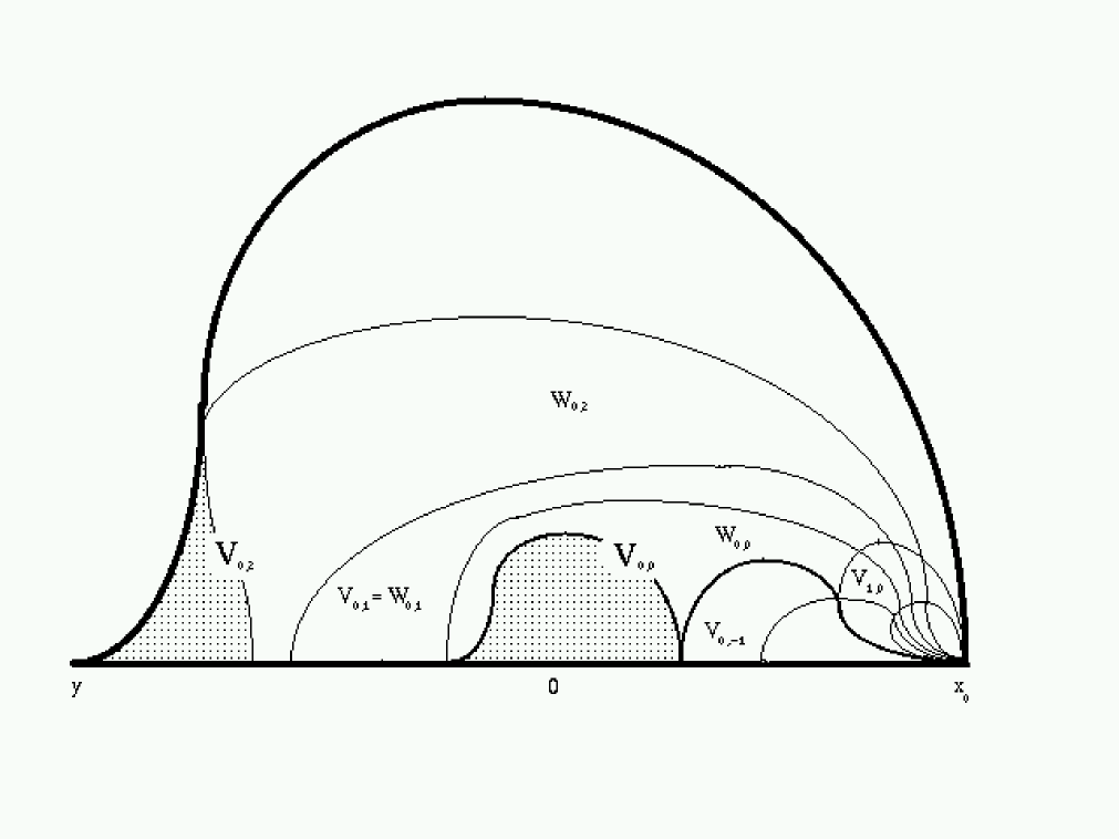
Figure 1: This is a schematic drawing of $\Omega_{-}\cap\mathbb{H}_{+}$ and regions inside it. Areas delineated with thicker lines represent $\tau^{-1}\Omega_{-}$ and $\tau^{-1}\Omega_{+}$. Shaded areas correspond under $G^{2}$.

The geometry of $H$.

See Figure 1 for an illustration and explanation of some notations.

Let us define $B=\Omega_{-}\setminus\tau^{-1}\overline{\Omega_{-}}$ and $B_{\pm}:=B\cap\mathbb{H}_{\pm}$. Then define $D_{\pm}=B_{\pm}\setminus\tau^{-1}\overline{\Omega_{+}}$.

A convenient parametrization of the set $\Omega_{-}$ is given by the map $h^{-1}$ from a slit plane $C_{h}$, as described by item (4) of Theorem 2. If we write $w=h(z)$, then the map $H(z)$ corresponds to $\exp(w)$ and, more strikingly $z\rightarrow G^{2}(z)$ is conjugated to $w\rightarrow w-2\log\tau$. Geometrically, it is worth noting that the beginning of the slit at $w=2\log\tau$ corresponds to the point $y$ in Figure 1 where the boundaries of $\Omega_{+}$ and $\Omega_{-}$ which follow the real line to the right of $y$, split.

Following [10], connected sets $V_{k,k^{\prime}}$, $k,k^{\prime}\in\mathbb{Z}$, are chosen in $\Omega_{-}$ so that each is mapped by $H$ onto $\tau^{k^{\prime}+1}B_{\pm}$.

More explicitly, in the $w$-coordinate

$$h(V_{k,k^{\prime}})=\{w\in C_{h}:\>\exp(w-k^{\prime}\log\tau)\in\tau B_{\pm},\,k\pi<\Im w<(k+1)\pi\}\;.$$

Now $\tau^{-1}\Omega_{-}\subset\overline{V_{0,0}\cup V_{-1,0}}$. Hence, for $k=0,-1$ and $k^{\prime}$ even and non-negative, $V_{k,k^{\prime}}$ contains the preimage of $\tau^{-1}\Omega_{-}$ by $G^{k^{\prime}}$. To exclude this preimage, if $k=0$ or $k=-1$ and $k^{\prime}$ is even end non-negative, we define $W_{k,k^{\prime}}=V_{k,k^{\prime}}\setminus G^{-k^{\prime}}(\tau^{-1}\Omega_{-})$. For all other pairs $(k,k^{\prime})$, $W_{k,k^{\prime}}=V_{k,k^{\prime}}$.

Rescaled map.

Let us define the “rescaled map” $\tilde{H}$ as follows.

• if $z\in W_{k,k^{\prime}}$, $(k,k^{\prime})\in\mathbb{Z}\times\mathbb{Z}$, then $\tilde{H}(z)=\tau^{-k^{\prime}-1}H(z)$,

• if $z\in V_{k,k^{\prime}}\setminus W_{k,k^{\prime}}$, $(k,k^{\prime})\in\{0,-1\}\times 2\mathbb{Z}_{+}$,

  then first consider $Z=G^{k^{\prime}}(z)$. $Z\in\overline{\tau^{-1}\Omega_{-}}$ which consists of the rescaled copies of $B_{\pm}$. Then $\tilde{H}(z)$ is defined if and only if $Z\in\tau^{-p}B_{\pm}$ for some $p>0$ and then $\tilde{H}(z)=\tau^{p}Z$.

Notice that this definition ensures that $\tilde{H}$ maps every connected component of its domain univalently onto one of the four possible pieces $D_{\pm},B_{\pm}$. The image is $B_{\pm}$ in the second case of the definition of the rescaled map and also in the first case whenever $W_{k,k^{\prime}}=V_{k,k^{\prime}}$.

On the other hand $\tilde{H}$ on $W_{0,0}$ is $\tau^{-1}H=\tau^{-1}G\tau$. It maps $W_{0,0}$ univalently onto $D_{-}$ since $G$ maps $\Omega_{-}$ onto $\Omega_{+}$. On $W_{-1,0}$, $\tilde{H}$ is the mirror reflection of this map, so the same formula actually holds. We will refer to $W_{0,0},W_{-1,0}$ as the central pieces.

On $W_{2p,0}$, $p>0$, $\tilde{H}=\tilde{H}_{|W_{0,0}}\circ G^{2p}$, so it also maps onto $D_{-}$ and similarly $W_{-1,2p}$ is mapped onto $D_{+}$.

Distortion properties of $\tilde{H}$ are given by Proposition 1 of [10]. As it turns out, most branches of $\tilde{H}^{n}$ can be be continued as univalent maps onto fixed neighborhoods of $B_{\pm},D_{\pm}$, fixed meaning independent of a branch or $n$, with the exception of those branches whose domains are send to the central pieces by $\tilde{H}^{n-1}$.

Towers.

The following is a trivial application of the concept of a tower used in [12].

Definition 2.1

Suppose we have a pair $(H,\tau)$ which satisfies the equation 1. For every $k\in\mathbb{Z}$, $H$ gives rise to a rescaled mapping $H_{k}(z)=\tau^{k}H(\tau^{-k}z)$. The set $\{H_{k}:\>k\in\mathbb{Z}\}$ will be called the tower of $H$. The set of all possible compositions of maps from a tower will be referred to as tower dynamics.

Towers will be used when $H$ could be the limiting map discussed in the previous paragraph, or one of the fixed point transformations $H^{(\ell)}$ of finite degree.

Tower dynamics forms a dynamical system, namely it defines an action of the semi-group of non-negative binary rational numbers under which integers correspond to ordinary iterates of $H$ and $2^{-k}$ acts as $H_{k}$. This follows from the following lemma.

Lemma 2.1

For every $k\in\mathbb{Z}$, $H_{k}^{2}=H_{k-1}$.

• Based on the functional equation 1,

  $$H_{k}\circ H_{k}(x)=\tau^{k-1}\tau H^{2}(\tau^{-1}(\tau^{-k+1}x))=\tau^{k-1}H(\tau^{-k+1}x)=H_{k-1}(x)\;.$$

  $\square$

2.2 Further inducing

Map $\tilde{H}$ has satisfactory properties from the combinatorial point view, since $B_{+}$ and $B_{-}$ are cut into countably many topological disks, each is of which is mapped univalently back onto $B_{+}$ or $B_{-}$. However, we would like it to have bounded distortion and that is generally not so. A standard approach to obtaining bounded distortion is by inducing and will follow that route now.

Start by introducing new pieces $K_{\pm}=B_{\pm}\setminus\overline{W_{0,0}\cup W_{-1,0}}$ and $L_{\pm}=D_{\pm}\setminus\overline{W_{0,0}\cup W_{-1,0}}$.

We will next define the map $\tilde{C}$ almost everywhere on the union of the central pieces, induced by $\tilde{H}=\tau^{-1}G\tau$, for which every branch maps on $L_{\pm}$. This will allow us to build the map $\tilde{J}$ defined on the domain of $\tilde{H}$ by $\tilde{H}$ except on $\tilde{H}^{-1}(W_{0,0}\cup W_{-1,0})$ and by $\tilde{C}\circ\tilde{H}$ otherwise.

The mapping $\tilde{C}$.

We will only consider $\tilde{C}$ on $W_{0,0}$. Mapping on $W_{-1,0}$ will be the mirror reflection.

By Lemma 2.13 in [10], no point will stay forever in $W_{0,0}$ under the iteration by $\tilde{H}$. Hence, $\tilde{C}$ is simply defined as the first entry map into $L_{+}$ under the iteration by $\tilde{H}$.

Lemma 2.2

Every branch of $\tilde{C}$ has a univalent extension onto a simply connected neighborhood $U_{L}$ of $L_{+}$. $U$ is the same for all branches of $\tilde{C}$ and its preimages by any branch is contained in the set $S:=\{z:\>\Re z<0\;\mbox{or}\;\Im z>0\}$.

• Since $\tilde{H}$ on $W_{0,0}$ is $G_{-1}=\tau^{-1}G\tau$ and $\overline{L_{+}}$ only intersects $\mathbb{R}_{+}$ at $x_{0}$ which is not a critical point of $\tilde{H}$, we can define and inverse branch on a neighborhood of $L_{+}$. Since the preimage of $\overline{L_{+}}$ by $G_{-1}$ now only intersects the real line at $y$, that neighborhood $U_{L}$ can be chosen to fit into $S$. This proved the needed extension for the branch of $\tilde{C}$ which is the first iterate of $\tilde{H}$. To examine further branches, continue mapping by the inverse branch of $\tilde{H}$ defined on $S$. From the properties of $G$, that inverse branch sends $S$ into itself, or even into the upper half plane.

  $\square$

Bounded distortion for $\tilde{J}$.

Now define map $\tilde{J}$ which equals $\tilde{H}$ everywhere on the domain of $\tilde{H}$ except on preimages to the central pieces and $\tilde{C}\circ\tilde{H}$ on such preimages.

Each branch of $\tilde{J}$ maps onto one of the pieces $K_{\pm},L_{\pm}$.

Proposition 1

There are fixed neighborhoods of sets $\overline{K_{\pm}}$ and $\overline{L_{\pm}}$ such that for any $n$ any branch of $\tilde{J}^{n}$ which maps onto one those sets can also be extended univalently so that it maps onto the corresponding neighborhood.

The map $\tilde{J}^{n}$ can be expended as a composition of $\tilde{H}$ and $\tilde{C}$ in which $\tilde{C}$ cannot be followed by another $\tilde{C}$. Since $\tilde{C}$ is also induced by $\tilde{H}$, we can use Proposition 1 from [10]. It asserts that if $\tilde{H}$ is the last mapping applied in this composition, then the claim of Proposition 1 holds. So consider the situation when $\tilde{C}$ is applied last. By Lemma 2.10 from [10], the entire composition that comes before it can be continued so that it maps onto $\mathbb{C}\setminus[0,+\infty)$. This obviously contains the set $S$ mentioned in Lemma 2.2, so again we get a univalent extension mapping over a fixed neighborhood of $\overline{L_{\pm}}$.

This proves Proposition 1.

By Köbe’s Lemma we now know that all branch of $\tilde{J}^{n}$ have distortion bounded uniformly with respect to $n$.

2.3 Tower Dynamics

By Lemma 2.14 from [10], for every branch $\zeta$ of $\tilde{H}$ there exists an integer $p$ such that $\tau^{p}\zeta$ belongs to the tower of $H$, see Definition 2.1. Let us call $p$ the combinatorial displacement of $\zeta$.

This leads to the following definition.

Definition 2.2

A mapping defined on an open set contained in the fundamental ring $\Omega_{-}\setminus\tau^{-1}\overline{\Omega_{-}}$ is called tower-induced if on each connected component of its domain it has the form $\tau^{q}h$ where $q$ is an integer and $h$ belongs to the tower of $H$.

For a tower-induced mapping, the choice of $q$ and $h$ is unique.

Lemma 2.3

If $\tau^{q}h=\tau^{q^{\prime}}h^{\prime}$ on a connected open set, with $q,q^{\prime}\in\mathbb{Z}$ and $h,h^{\prime}$ in the tower of $H$, then $q=q^{\prime}$ and $h=h^{\prime}$.

• Both $h$ and $h^{\prime}$ are iterates of the same $h_{0}$ in the tower, say $h=h_{0}^{m},h^{\prime}=h_{0}^{m^{\prime}}$, $m,m^{\prime}>0$. Without loss of generality, $m^{\prime}\geq m$. Then

  $$\tau^{q-q^{\prime}}=h_{0}^{m^{\prime}-m}$$

  on an open set, but this is impossible given that no iterate of $h_{0}$ is a linear map.

  $\square$

Definition 2.3

Given a tower-induced map $\Phi$ on a subset $U$ of the fundamental ring, we can define its associated map as follows. On $U$, wherever $\Phi=\tau^{q}h$, the associated map is just $h$. On $\tau^{p}U$, where $p\in\mathbb{Z}$, the associated map is $\tau^{p}h\tau^{-p}$.

In this way, the associated map belongs to the tower.

Lemma 2.4

If the combinatorial displacement of a tower induced map is $q$ at some point $x$, then for any $p\in\mathbb{Z}$ the associated map sends $\tau^{p}x$ in $\tau^{p+q}(\Omega_{-}\setminus\tau^{-1}\overline{\Omega_{-}})$.

• It is a direct consequence of the definitions.

  $\square$

Lemma 2.5

If $\zeta_{1}$ and $\zeta_{2}$ are two tower-induced mappings with associated maps $\Theta_{1},\Theta_{2}$, respectively, then $\zeta_{1}\circ\zeta_{2}$ is also a tower-induced map with the associated map $\Theta_{1}\circ\Theta_{2}$.

• Denote $\zeta_{1}=\tau^{q_{1}}h_{1},\zeta_{2}=\tau^{q_{2}}h_{2}$. Without loss of generality, the domain of $\zeta_{2}$ is connected and so $q_{2}$ is constant, while $q_{1}$ is only piecewise constant and $h_{1}$ is only piecewise a map from the tower.

  Then

  $$\zeta_{1}\circ\zeta_{2}=\tau^{q_{1}}h_{1}\tau^{q_{2}}h_{2}=\tau^{q_{1}+q_{2}}(\tau^{-q_{2}}h_{1}\tau^{q_{2}})h_{2}\;.$$

  Mappings $h_{2}$ and $\tau^{-q_{2}}h_{1}\tau^{q_{2}}$ both belong to the tower and so does their composition. Thus, the composition $\zeta_{1}\circ\zeta_{2}$ is tower-induced and its associated map is $(\tau^{-q_{2}}h_{1}\tau^{q_{2}})h_{2}$ on the domain of $\zeta_{2}$. On the other hand, $h_{2}$ maps the domain of $\zeta_{2}$ into $\tau^{-q_{2}}(\Omega_{-}\setminus\tau^{-1}\Omega_{-})$. So, the composition of the associated maps is indeed

  $$(\tau^{-q_{2}}h_{1}\tau^{q_{2}})h_{2}$$

  on the domain of $\zeta_{2}$. So, the associated map of the composition is equal to the composition of the associated maps on the domain of $\zeta_{2}$. When considered on rescaled images of the domain of $\zeta_{2}$, both $\Theta_{1}\circ\Theta_{2}$ and the associated map of $\zeta_{1}\circ\zeta_{2}$ are equivariant with respect to such rescalings, so the equality holds everywhere.

  $\square$

As a consequence of Lemma 2.4 and Lemma 2.5, combinatorial displacements are additive under the composition of tower-induced maps.

Dynamical interpretation of $\tilde{J}$.

Let us recall the mapping $\tilde{J}$ defined previously. Map $\Lambda$ is equal to $\tilde{J}$ except on $\tau^{-1}\Omega_{+}$, where we modify the definition to ${\tilde{J}}\circ{\tilde{J}}$.

Proposition 2

If $x$ belongs to the Julia set of $H$ and to the domain of $\Lambda^{p}$, $p>0$, then the map associated to $\Lambda^{p}$ is equal to an iterate of $H$ on a neighborhood of $x$.

Throughout this proof we assume that $x$ belongs to the Julia set of $H$.

We split the proof depending on whether $x$ belongs to $\Omega_{+}$ or $\Omega_{-}$.

The first case to consider is $x\in\Omega_{+}$. To determine the map associated to $\Lambda$ on a neighborhood of $x$, we need to look at $\Lambda$ on a neighborhood of $\tau^{-1}x\in\tau^{-1}\Omega_{+}$. By the modification we just described, $\Lambda$ is ${\tilde{J}}^{2}$ on a neighborhood of $\tau^{-1}x$ and so the associated map at $\tau^{-1}x$, as well as $x$, is the associated map of ${\tilde{J}}$ composed with itself.

On $\Omega_{+}$ the associated map $\tilde{J}$ is $H_{1}=\tau H\tau^{-1}$. Then we know that $H_{1}(H_{1}(x))=H(x)$ is in $\Omega_{-}\cup\Omega_{+}\subset\tau\Omega_{-}$. i.e. $H_{1}(x)\in H_{1}^{-1}(\tau\Omega_{-})\cap\tau\Omega_{-}$ or $\tau^{-1}H_{1}(x)\in H^{-1}(\Omega_{-})\cap\Omega_{-}$. It follows that ${\tilde{J}}$ on a neighborhood of ${\tilde{J}}(\tau^{-1}x)=\tau^{-1}H_{1}(x)$ is $H$, and therefore its associate map at $H_{1}(x)$ is $H_{1}$ again. So, by Lemma 2.5, the associated map of $\Lambda$ is $H_{1}\circ H_{1}=H$ in a neighborhood of $x$.

Let us now consider $x\in\Omega_{-}$.

Since ${\tilde{J}}={\tilde{C}}\circ{\tilde{H}}$, with both $\tilde{C}$ and $\tilde{H}$ tower-induced maps, we have an analogous decomposition of the map $\Phi_{J}$ associated to $\tilde{J}$ into the composition of $\Phi_{H}$ associated to $\tilde{H}$ and $\Phi_{C}$ associated to $\tilde{C}$.

Lemma 2.6

Suppose $x\in\Omega_{-}$. Then $\Phi_{C}$ on a neighborhood of $x$ is an iterate of $H_{-1}$.

• $\tilde{C}$ is induced by the map $G_{-1}=\tau^{-1}H$. So, the associated map is $H$ on the fundamental ring $\Omega_{-}\setminus\tau^{-1}\overline{\Omega_{-}}$. However, the combinatorial displacement of $G_{-1}$ is $1$, so by Lemma 2.2 the map associated to ${\tilde{C}}^{2}$ is $H_{1}\circ H$ and, inductively, the map associated to ${\tilde{C}}^{k}$, $k\geq 1$, is $H_{k-1}\circ\cdots\circ H$ wherever ${\tilde{C}}^{k}$ is defined on the fundamental ring.

  Observe that $H$ maps any point in the domain of ${\tilde{C}}$ outside of $\Omega_{-}\cup\Omega_{+}$. Hence, no $x$ from the Julia set of $H$ can be found there. However, we may encounter points from the Julia set on the domain of ${\tilde{C}}$ rescaled by $\tau^{-p}$, $p>0$. By the equivariance with respect to the rescaling by $\tau$, the map associated to ${\tilde{C}}^{k}$ on a neighborhood of such a point is $H_{k-1-p}\circ\cdots\circ H_{-p}$. Again, this composition cannot contain $H_{0}=H$ which would eject the point out of the Julia set, hence $k-1-p<0$, hence $\Phi_{C}$ is generated by $H_{-1}$ in the neighborhood of $x$.

  $\square$

In the light of Lemma 2.6 in order to conclude that $\phi_{C}\circ\Phi_{H}$ is an iterate of $H$ in a neighborhood of $x$ it will be enough to show that $\Phi_{H}$ is an iterate of $H$ on such a neighborhood. Then, $\Phi_{H}(x)$ is in the Julia set of $H$ and Lemma 2.6 is applicable.

${\tilde{H}}$ is simply $\tau^{q}H$ on most of its domain, with the sole exception of domains $G^{-2k}(\tau^{-1}\Omega_{-})$ where the inverse branch of $G$ which fixes $x_{0}$ is used. On any such domain, $\tilde{H}$ is $\tau^{q}G^{2k}$. Since $G=\tau^{-1}H_{1}$ its associated map is $H_{1}$ and the combinatorial displacement is $1$. Hence, the map associated to $\tilde{H}$ on such a domain is

$$H_{2k}\circ H_{2k-1}\circ\cdots\circ H_{1}\;.$$ (2)

Also,

$$H(G^{-2k}(\tau^{-1}\Omega_{-}))=\tau^{2k}H\tau^{-1}(\Omega_{-})=\tau^{2k}G(\Omega_{-})=\tau^{2k}\Omega_{+}\;.$$

Now take $x$ in the Julia and in $\tau^{-p}(\Omega_{-}\setminus\tau^{-1}\overline{\Omega_{-}})$. Without loss of generality $p\geq 0$ since the case of $x\in\Omega_{+}$ was already considered. If $x$ is not in the rescaled image of one of the exceptional domains discussed in the previous paragraph, then the map associated to $\tilde{H}$ is just $H_{-p}$.

If $x$ is in $\tau^{-p}G^{-2k}(\tau^{-1}(\Omega_{-}))$, then $H_{-p}$ maps it into$\tau^{2k-p}\Omega_{+}$. But $H_{-p}$ is an iterate of $H$, so it has to map $x$ into the Julia set of $H$ and thus $2k-p\leq 0$ or $2k\leq p$. By formula (2), the associated map is given by

$$\tau^{p}H_{2k}\circ\cdots\circ H_{1}\tau^{-p}$$

which is clearly generated by $\tau^{p}H_{2k}\tau^{-p}=H_{2k-p}$, thus by $H_{0}$ in view of the inequality $2k\leq p$.

What we now proved is that if $x\in\Omega_{-}$, then the map associated to ${\tilde{J}}$ is an iterate of $H$ on a neighborhood. This is the same as the map associated to $\Lambda$ unless $x\in\tau^{-1-p}\Omega_{+}$ for $p\geq 0$. If that happens, $\Lambda={\tilde{J}}\circ{\tilde{J}}$ and the map associated to $\tilde{J}$ is $H_{-p}$ on a neighborhood of $x$ and therefore maps $x$ into $\tau^{-p}\Omega_{-}$. Then, again the map associated to the second iterate of $\tilde{J}$ is generated by $H$ on a neighborhood of $H_{-p}(x)$.

Proposition 2 has been demonstrated.

3 Drift Estimates

3.1 Martingale estimates

We will be using the following abstract probabilistic statement. Its stronger form under stronger conditions can be found in the literature, see the discussion and references in the Introduction.

Define $\gamma_{k}(x)=x\chi_{[-k,k]}(x)$ for $k>0$.

Proposition 3

On a certain probability space $\Omega$ with measure $\mu$ consider an integer-valued stochastic process $(Z_{n})_{n=0}^{\infty}$. Let ${\cal F}_{n}$ denote the $\sigma$-algebra generated by $Z_{0},\cdots,Z_{n}$. For $n\geq 1$, let $F_{n}=Z_{n}-Z_{n-1}$. Assume that for each $n\geq 1$ we have a decomposition $F_{n}=\Delta_{n}+I_{n}$, with $\Delta_{n}$ and $I_{n}$ both integer-valued. Moreover, assume that positive constants $K_{1},K_{2}$, $p>1$, exist with which the following estimates hold for every $n\geq 1$:

• for every $k\in\mathbb{Z},k\neq 0$

  $$K_{1}^{-1}k^{-2}\leq P({\Delta_{n}=k}|{\cal F}_{n-1})(\omega)\leq K_{1}k^{-2}$$

  for $\mu$-almost all $\omega$,

• for every positive $k$,

  $$|E(\gamma_{k}(\Delta_{n})|{\cal F}_{n-1})(\omega)|\leq K_{2}$$

  almost surely,

• $$E(|I_{n}|^{p}){\cal F}_{n-1})(\omega)\leq K^{p}_{2}$$

  almost surely.

Then, $\mu$-almost surely $\lim\sup_{n\rightarrow\infty}\frac{Z_{n}}{n}=+\infty$ and $\lim\inf_{n\rightarrow\infty}\frac{Z_{n}}{n}=-\infty$.

Let us define $\log^{+}(x)$, $x\in\mathbb{R}$ to be $\log(x)$ if $x>1$ and $0$ otherwise.

Lemma 3.1

Consider a probability space $P$ with measure $\mu$. Let $\Delta$ and $I$ be integer-valued random variables and $F=\Delta+I$. Assume that for some $Q^{\prime},Q^{\prime\prime}>0$, $p>1$ and every $k\neq 0$:

• $$(Q^{\prime}k^{2})^{-1}\leq\mu({\Delta=k})\leq Q^{\prime}k^{-2}\;,$$

• if $k>0$, then

  $$|E(\gamma_{k}(\Delta))|\leq Q^{\prime\prime}\;,$$

• $$E(|I|^{p})\leq(Q^{\prime\prime})^{p}$$

There exists $Q_{0}>1$ which only depends on $Q^{\prime},Q^{\prime\prime},p$ such that for every $Q\geq Q_{0}$

$$E(\log^{+}(Q+F))<\log Q\;.$$

• Without loss of generality we can replace $I(x)$ with $\max(I(x),0)$. i.e. assume that $I(x)$ is a non-negative function.

  Assume $Q>800$ and distinguish sets $X_{Q}:=\{x\in P:\>Q+\Delta(x)>1\}$ and $Y_{Q}:=\{x\in P:\>|\Delta(x)|\leq Q\log Q-Q\}$.

$$\int_{P\setminus Y_{Q}}\log^{+}(Q+F(x))\,d\mu(x)\leq\int_{X_{Q}\setminus Y_{Q}}\log^{+}(Q+F(x))\,d\mu(x)+$$

$$+\int_{P\setminus(Y_{Q}\cup X_{Q})}\log^{+}\left[I(x)-Q(\log Q-2)\right]\,d\mu(x)$$

since on the complement of $X_{Q}\cup Y_{Q}$ we have $\Delta(x)<-Q\log Q+Q$.

To estimate that last term, denote $S=\{x\in P\setminus(Y_{Q}\cup X_{Q}):I(x)\geq Q(\log Q-2)+1)$. Using Jensen’s inequality for conditional expectations

$$\int_{P\setminus(Y_{Q}\cup X_{Q})}\log^{+}\left[I(x)-Q(\log Q-2)\right]\,d\mu(x)\leq\int_{S}\log I(x)\,d\mu(x)=$$

$$=\mu(S)E(\log I(x)|x\in S)\leq\mu(S)\log E(I(x)|x\in S)\;.$$

Furthermore,

$$E(\log I(x)|x\in S)\leq\frac{E(I)}{\mu(S)}\leq\frac{Q^{\prime\prime}}{\mu(S)}$$

and

$$\mu(S)\log E(I(x)|x\in S)\leq\mu(S)\log Q^{\prime\prime}-\mu(S)\log(\mu(S))\;.$$

Since $Q>800$, we have

$$\frac{Q}{2}\log Q\cdot\mu(S)<Q(\log Q-2)\mu(S)<\int_{S}I(x)\,d\mu(x)\leq Q^{\prime\prime}$$

which implies $\mu(S)<\frac{2Q^{\prime\prime}}{Q\log Q}$ and from the previous estimate

$$\int_{P\setminus(Y_{Q}\cup X_{Q})}\log^{+}\left[I(x)-Q(\log Q-2)\right]\,d\mu(x)\leq$$

$$\leq\frac{2Q^{\prime\prime}\log Q^{\prime\prime}}{Q\log Q}+\frac{2Q^{\prime\prime}}{Q\log Q}(\log Q+\log\log Q-\log(2Q^{\prime\prime}))\leq\frac{Q^{\prime}_{1}}{Q}$$

for an appropriately chosen constant $Q^{\prime}_{1}$ which only depends on $Q^{\prime\prime}$.

$$\int_{P\setminus Y_{Q}}\log^{+}(Q+F(x))\,d\mu(x)\leq\frac{Q^{\prime}_{1}}{Q}+\int_{X_{Q}\setminus Y_{Q}}\log(Q+\Delta(x))\,d\mu(x)+$$

$$+\int_{X_{Q}\setminus Y_{Q}}\frac{I(x)}{Q+\Delta(x)}\,d\mu(x)\leq\frac{Q^{\prime}_{1}}{Q}+\sum_{n>Q\log Q}Q^{\prime}\log(Q+n)n^{-2}+\frac{Q^{\prime\prime}}{Q}$$

$$\leq\frac{Q^{\prime}_{1}}{Q}+\frac{Q^{\prime\prime}}{Q}+2Q^{\prime}\sum_{n\geq Q\log Q}\log(n)n^{-2}\leq Q_{1}Q^{-1}$$ (3)

where the final estimate arises from an explicit integration of the function $x^{-2}\log x$ and $Q_{1}$ only depends on $Q^{\prime}$ and $Q^{\prime\prime}$.

Let $\lambda_{Q}$ denote the affine function tangent to $\log x$ at $Q$, i.e. $\lambda_{Q}(x)=\log Q+\frac{x}{Q}-1$. Then

$$\int_{Y_{Q}}\log^{+}(Q+F(x))\,d\mu(x)=$$ (4)

$$=\int_{Y_{Q}}\lambda_{Q}(Q+F(x))\;d\mu(x)-\int_{Y_{Q}}(\lambda_{Q}-\log^{+})(Q+F(x))\,d\mu(x)\;.$$

As to the first term, we estimate

$$\int_{Y_{Q}}\lambda_{Q}(Q+F(x))\;d\mu(x)=$$

$$=\log(Q)\mu(Y_{Q})+\frac{1}{Q}\int_{Y_{Q}}F(x)\,d\mu(x)-1<\log(Q)+(2Q^{\prime\prime})Q^{-1}$$

Taking this into account together with estimates (3) and (4), we get

$$\int_{P}\log^{+}(Q+F(x))\,d\mu(x)-\log Q<\frac{Q_{1}+2Q^{\prime\prime}}{Q}-$$ (5)

$$-\int_{Y_{Q}}\left(\lambda_{Q}-\log^{+})(Q+F(x)\right)\,d\mu(x)\;.$$

The rest of the proof will consist in estimating the final negative term in (5) to show that it goes to $0$ as $Q\rightarrow\infty$ more slowly than $O(Q^{-1})$ and hence prevails for sufficiently large $Q$. The values of $\lambda_{Q}(x)$ remain above $\log_{+}(x)$ for $x>-Q\log Q+Q$. Since $I(x)$ is non-negative and $\Delta(x)\geq-Q\log Q+Q$ on $Y_{Q}$, $(\lambda_{Q}-\log^{+})(Q+F(x))$ is non-negative on $Y_{Q}$. Choose $Z_{Q}:=\{x\in P:\>-3Q<\Delta(x)<-2Q\}$. Since $Q>800$, $Z_{Q}\subset Y_{Q}$ and

$$\int_{Y_{Q}}\left(\lambda_{Q}-\log^{+})(Q+F(x)\right)\,d\mu(x)\geq\int_{Z_{Q}}\left(\lambda_{Q}-\log^{+})(Q+F(x)\right)\,d\mu(x)$$ (6)

For $Q>800$ and $x\in Z_{Q}$,

$$\lambda_{Q}(Q+\Delta(x))\geq\log Q-3>\frac{\log Q}{2}\;.$$

At the same time, for $x\in Z_{Q}$,

$$Q+F(x)=Q+\Delta(x)+I(x)<I(x)-Q\ .$$

Hence,

$$\int_{Z_{Q}}\left(\lambda_{Q}-\log^{+}\right)(Q+F(x))\,d\mu(x)>$$

$$>\frac{\log Q}{2}\mu(Z_{Q})+\int_{Z_{Q}}\left[\frac{I(x)}{Q}-\log^{+}(I(x)-Q)\right]\,d\mu(x)\;.$$

By the hypothesis of the lemma, $\mu(Z_{Q})>2Q_{2}/Q$ for some positive $Q_{2}$ where $Q_{2}$ depends only on $Q^{\prime\prime}$ and so

$$\int_{Z_{Q}}\left(\lambda_{Q}-\log^{+}\right)(Q+F(x))\,d\mu(x)>$$

$$>Q_{2}\frac{\log Q}{Q}+\int_{Z_{Q}}\left[\frac{I(x)}{Q}-\log^{+}(I(x)-Q)\right]\,d\mu(x)\;.$$

In the integral term, the integrand is non-negative if $I(x)\leq Q+1$ or $I(x)\geq Q^{2}$, keeping in mind that $Q>800$. For other values of $x$, the lower bound by $-\log Q^{2}$ holds. It follows that

$$\int_{Z_{Q}}\left[\frac{I(x)}{Q}-\log^{+}(I(x)-Q)\right]\,d\mu(x)>-\log Q^{2}\mu(\{x:\>Q<I(x)<Q^{2}\})\;.$$

Since

$$\int_{Q<I(x)<Q^{2}}I^{p}(x)\,d\mu(x)>(Q^{\prime\prime})^{p}\mu(\{x:\>Q<I(x)<Q^{2}\}\;,$$

one gets

$$\mu(\{x:\>Q<I(x)<Q^{2}\})<\frac{(Q^{\prime\prime})^{p}}{Q^{p}}$$

Thus,

$$\int_{Z_{Q}}\left(\lambda_{Q}-\log^{+}\right)(Q+F(x))\,d\mu(x)>Q_{2}\frac{\log Q}{Q}-2\frac{(Q^{\prime\prime})^{p}}{Q^{p-1}}\frac{\log Q}{Q}>\frac{Q_{2}}{2}\frac{\log Q}{Q}$$

for $Q\geq Q_{0}=(\frac{4(Q^{\prime\prime})^{p}}{Q_{2}})^{\frac{1}{p-1}}$.

Hence for $Q\geq Q_{0}$, in view of (6), the negative term on the right-hand side of estimate (5) dominates and that proves the assertion of Lemma 3.1.

$\square$

Lemma 3.1 will be used with $Q^{\prime}=K_{1}$ and $Q^{\prime\prime}=K_{2}$ from Proposition 3. This defines a constant $Q_{0}$.

Supermartingale construction.

Choose $N\geq 0$. Under the hypothesis of Proposition 3, define a stochastic process $(\zeta_{n}^{(N)})_{n\geq N}$ as follows. If for some $N\leq k\leq n$, $Z_{n}(x)<Q_{0}$, then pick the smallest such $k$ and set $\zeta_{n}^{(N)}(x)=\log^{+}Z_{k}(x)$. Otherwise, let $\zeta_{n}^{(N)}(x)=\log Z_{n}(x)$. In other words, $\zeta_{n}^{(N)}$ is the process $\log^{+}Z_{n}$ starting at $N$ and stopped when $Z_{n}$ first dips below $Q_{0}$.

Lemma 3.2

For every $N\geq 0$, $\zeta_{n}^{(N)}$ is a supermartingale with respect to the filtration $({\cal F})_{n}$ and converges almost surely to a finite limit.

• If $\zeta_{n-1}^{(N)}<\log Q_{0}$, then the process is stopped and its conditional increment is $0$. Otherwise, if $\zeta_{n-1}^{(N)}=\log Q\geq\log Q_{0}$, Lemma 3.1 can be applied to the conditional increments. That, we put $F,\Delta,I$ equal to $F_{n},\Delta_{n},I_{n}$, respectively and the probabilistic space is the set $S=\{\omega:\>\zeta_{n-1}^{(N)}(\omega)=Q\}$ with normalized measure $\mu$. Then the Lemma says that $E(\zeta_{n}^{(N)}-\log Q|{\cal F}_{n-1})(\omega)<0$ almost surely on $S$.

  Since $\zeta_{n}^{(N)}$ is non-negative by definition, it converges almost surely by martingale theory.

  $\square$

Proof of Proposition 3.

We will first show that $\lim_{n\rightarrow\infty}Z_{n}=+\infty$ with probability $0$. Suppose otherwise. Then there is $N$ such that with positive probability $Z_{n}(x)>Q_{0}$ for all $n\geq N$ and $\lim_{n\rightarrow\infty}Z_{n}(x)=+\infty$. Considering $\zeta_{n}^{(N)}$ we see that on this set $\zeta_{n}^{(N)}(x)=\log Z_{n}(x)$ for all $x$ and thus diverges to $\infty$ contrary to the assertion of Lemma 3.2.

Now pick an arbitrary $M>0$ and consider the process $\tilde{Z}_{n}=Z_{n}+nM$. It is measurable with respect to the same filtration $({\cal F})_{n}$ and evidently satisfies the hypothesis of Proposition 3, since we can just set $\tilde{I}_{n}=I_{n}+M$ for all $n$. The hypothesis of Proposition 3 is satisfied with the same $K_{1}$ and $K_{2}:=K_{2}+M$. Hence, the conclusion that $\lim_{n\rightarrow\infty}\tilde{Z}_{n}=\infty$ almost nowhere remains valid.

But that means $Z_{n}<-Mn/2$ infinitely often almost surely, and so

$$\lim\inf_{n\rightarrow\infty}\frac{Z_{n}}{n}\leq M/2\;.$$

Since $M$ was arbitrary, we further conclude that

$$\lim\inf_{n\rightarrow\infty}\frac{Z_{n}}{n}=-\infty$$

almost surely and by considering the process $(-Z_{n})$ instead of $(Z_{n})$, we also get that the upper limit of $\frac{Z_{n}}{n}$ is $+\infty$ almost surely.

3.2 The drift function

Based on Lemma 2.5 we can define combinatorial displacements for all branches induced by $\tilde{H}$ by simply adding the displacements for all branches of $\tilde{H}$ that occur in the composition. It will then remain true that if a branch $\zeta$ of the induced map has combinatorial displacement $p$, then $\tau^{p}\zeta$ belongs to the tower.

Definition 3.1

Given a map ${\cal J}$ induced by $\tilde{H}$, define its drift function $\Delta_{\cal J}$ to be equal on the domain of any branch of $\cal J$ to the combinatorial displacement of that branch.

Define

$$\gamma_{n}(x):=\left\{\begin{array}[]{ccc}0&\mbox{if}&x\geq n\\ x&\mbox{if}&-n<x<n\\ 0&\mbox{if}&x\leq-n\;.\end{array}\right.$$

Fix one of the four pieces $K_{\pm},L_{\pm}$ and denote it $P$. The set $M_{P}$ consists of all probabilistic measures $\mu$ on $P$ which can be obtained as $\mu=\zeta_{*}(Q\lambda)$ where $\zeta$ is a branch of $\tilde{J}^{n}$, for any $n\geq 1$, which maps onto $P$, $\lambda$ is the Lebesgue measure and $Q$ a normalizing constant equal to the reciprocal of the area of the domain of $\zeta$.

Define the function $\Delta^{0}$ as follows: $\Delta^{0}(z)=n$ if $z\in V_{k,n}$ for $k\neq 0,1$ and $n\in\mathbb{Z}$ and $0$ otherwise. Then $\Delta^{0}$ coincides with $\Delta_{\tilde{H}}$ except on the “central rows” $V_{k,n}$, $k=0,-1$. The idea of the proposition to follow is that $\Delta^{0}$ is a good approximation of the much more complicated function $\Delta_{\cal J}$ and that $\Delta^{0}$ has certain helpful properties.

Proposition 4

If $P$ is one of $K_{\pm},L_{\pm}$, then there exist positive $Q_{1},Q_{2},Q_{3}$ so that for every $\mu\in M_{P}$:

• $$\int_{P}|\Delta_{\tilde{\cal J}}-\Delta^{0}|^{\frac{3}{2}}\,d\mu<Q_{1}\;,$$

• for every $n\neq 0$,

  $$Q_{2}^{-1}|n|^{-2}<\mu(\{x\in P:\>\Delta^{0}=n\})<Q_{2}|n|^{-2}\;,$$

• for all $n$

  $$|\int_{P}\gamma_{n}\circ\Delta^{0}\,d\mu|\leq Q_{3}\;.$$

Observe that the first two properties would be enough to prove for the Lebesgue measure instead of $\mu$, since the densities $\frac{d\mu}{d\lambda}$ bounded for all $\mu\in M_{P}$ in view of bounded distortion.

The last property deserves attention. Although $\Delta^{0}$ is non-integrable in view of the second claim, its integrals in a certain principal value sense remain bounded. Also, this one would not be enough to prove for the Lebesgue measure as it involves cancellations.

Proof of Proposition 4.

Let us start with the following general Lemma.

Lemma 3.3

Let $\Phi$ be a holomorphic function defined on a neighborhood of $0$, with the power series expansion at $0$ in the form

$$\Phi(z)=z+az^{3}+O(|z|^{4})$$

with some complex $a\neq 0$. Choose $\tilde{h}$ to be its Fatou coordinate, so that

$$\tilde{h}\circ\Phi(z)=\tilde{h}(z)+1$$

for all $z$ in an attracting petal of $0$. Let $f,g$ be continuous functions defined for $x>r>0$ for some $r$ such that $f(x)>g(x)$ for all $x$ and $1$-periodic.

There exists $K$ so that for any $n>r$ the area of the set

$$\tilde{h}^{-1}(\{x+iy:\>n<x<n+1,g(x)<y<f(x)\})$$

is bounded above by $Kn^{-3}$.

• It is well known (see also the proof of Lemma 3.7) that the

  $$|(\tilde{h}^{-1})^{\prime}(z)|=\tilde{L}|z|^{-3/2}+o(|z|^{-3/2})\;.$$

  Hence, the preimage by $\tilde{h}$ of any square

  $$\{x+iy:\>n<x<n+1,c<y<c+1\}$$

  for $n$ large has area bounded by $K_{1}n^{-3}$ and the hypotheses of continuity and 1-periodicity for $f,g$, any region in the form $\{x+iy:\>n<x<n+1,g(x)<y<f(x)\}$ is contained in the union of $m$ such squares with $m$ independent of $n$.

  $\square$

Observe that under $\tilde{h}^{-1}$, the graphs of $f$ and $g$ are mapped to curves invariant under $\Phi$ and tangent to the attracting direction of $\Phi$ at $0$ and, conversely, any two such curves give rise to functions, $f,g$ which satisfy the hypotheses of Lemma 3.3.

Lemma 3.4

Function $\Delta_{\tilde{C}}^{\frac{3}{2}}$ is integrable with respect to the Lebesgue measure on $W_{0,0}$.

• By the definition of $\tilde{C}$, $\Delta_{\tilde{C}}(z)$ is equal to the number of iterates of $\tilde{H}=\tau^{-1}G\tau$ needed to map $z$ outside of $W_{0,0}\cup W_{-1,0}$, which is bounded above by twice the number of iterates of $\tilde{H}^{2}$ needed to map $z$ outside of $W_{0},0$. $\tilde{H}$ has a degenerate neutral fixed point at $\tau^{-1}x_{0}$ in a neighborhood of the fixed point $W_{0,0}$ is just the complement of $\tau^{-1}(\Omega_{-}\cup\Omega_{+})$ whose boundary is mapped invariant under $G^{2}$ if neighborhood is small enough. Once $z$ leaves that fixed neighborhood of the fixed point, it will leave $W_{0,0}$ after a bounded number of further iterations. If we apply Lemma 3.3 to $\Phi:=\tilde{H}^{-1}$ we get that the measure of the set $S_{n}$ of points $z$ which stay in the neighborhood for exactly $n$ iterates of $\tilde{H}^{2}$ is bounded by $Kn^{-3}$. Since $\Delta_{\tilde{C}}$ on $S_{n}$ is bounded by $n$ plus a $Q$, the the integral of $\Delta_{\tilde{C}}^{\frac{3}{2}}$ over $W_{0,0}$ is bounded by

  $$2C|W_{0,0}|+2K\sum n^{-\frac{3}{2}}<\infty\;.$$

  $\square$

Lemma 3.5

For a certain $Q_{4}$

$$\int_{P}|\Delta_{\tilde{\cal J}}-\Delta_{\tilde{H}}|^{\frac{3}{2}}\,d\lambda<Q_{4}\;.$$

• Since $\tilde{\cal J}$ is either $\tilde{H}$, or $\tilde{C}\circ\tilde{H}$ if $\tilde{H}$ maps into $W_{0,0}\cup W_{-1,0}$,

  $$\Delta_{\tilde{\cal J}}=\Delta_{\tilde{H}}+\Delta_{\tilde{C}}$$

  where we put $\Delta_{\tilde{C}}$ equal to $0$ outside the domain of $\tilde{C}$.

$$\int_{P}|\Delta_{\tilde{\cal J}}-\Delta_{\tilde{H}}|^{\frac{3}{2}}\,d\lambda=\int_{P}|\Delta_{\tilde{C}}(\tilde{H}(z))|^{\frac{3}{2}}\,d\lambda(z)=$$

$$=\int_{(W_{0,0}\cup W_{0,-1})\cap P}|\Delta_{\tilde{C}}(w)|^{\frac{3}{2}}|(H^{-1})^{\prime}(w)|^{3}\,d\lambda(w)\;.$$

The derivative of $\tilde{H}^{-1}$ is bounded on the central pieces, since $\tilde{H}$ is univalent and maps onto a neighborhood of their closure. Thus, $\Delta_{\tilde{C}}$ is multiplied by a bounded factor and hence, in view of Lemma 3.4, the integral is finite.

$\square$

Lemma 3.6

There is $Q_{5}$ so that

$$\int_{P}|\Delta_{\tilde{H}}-\Delta^{0}|^{\frac{3}{2}}\,d\lambda<Q_{5}\;.$$

• Let $\chi_{0}$ be the characteristic function of the “central rows”, i.e. the union of pieces $V_{k,n}$, $k=0,-1$, $n\in\mathbb{Z}$.

  Clearly,

  $$\Delta_{\tilde{H}}-\Delta^{0}=\chi_{0}\Delta_{\tilde{H}}\;.$$

  Recall that on $W_{0,k},W_{-1,k}$, the combinatorial displacement is just $k$. When $k$ is positive and even, then $G^{k}$ is used to map $V_{0,k}\setminus W_{0,k}$ onto $\tau^{-p}B_{+}$ and the combinatorial displacement is $k-p$. The dynamics on $V_{-1,k}$ is the mirror image of this. On $V_{0,k}$, $\Delta_{\tilde{H}}$ is $k-p(z)$ where $p(z)$ is zero unless $k$ is positive and even, in which case it given by the condition $z\in G^{-k}\tau^{-p(z)}B_{+}$. Now $G^{k-1}$ maps $W_{0,k}$ with bounded distortion into a neighborhood of $\tau x_{0}$, which is the critical of $G$. Since $G^{k}$ is univalent on $W_{0,k}$, it follows that the area of the set of $z\in V_{0,k}$ such that $p(z)=p$ is bounded by $Q_{1}|V_{0,k}||p|^{-3}$. It follows that the integral of $|\Delta_{\tilde{H}}|^{\frac{3}{2}}$ over $V_{0,k}$ is bounded by $|V_{0,k}|(|k|^{\frac{3}{2}}+10Q_{1})$. By Lemma 3.3, $|V_{0,k}|\leq Kk^{-3}$ so that integral of $|\Delta_{\tilde{H}}|^{\frac{3}{2}}$ over the union of all pieces $V_{0,k},k\in\mathbb{Z}$ is finite. The same reasoning is applied to pieces $V_{-1,k}$.

  $\square$

From Lemmas 3.5 and 3.6, we derive the first claim of Proposition 4.

We will now deal with the remaining two claims which are only concerned with the function $\Delta^{0}$.

Start by defining sets $V_{n}=\bigcup_{k\not=0,-1}V_{k,n}$.

Lemma 3.7

There exist $C,K_{1}>0$, such that for all $n$

$$\lambda(V_{n})-C|n|^{-2}\leq K_{1}|n|^{-5/2}\;.$$

• Consider the map $h^{-1}$ from the slit plane $C_{h}$ onto $\Omega_{-}$ as described by item (4) of Theorem 2. The measure of $V_{n}$ is equal to the integral of $|(h^{-1})^{\prime}|^{2}$ over the set $S_{n}\cup\bar{S}_{n}$, where $\bar{S}_{n}=\{z:\bar{z}\in S_{n}\}$ is the mirrow symmetric to $S_{n}$ set, and $S_{n}$ is a set in the upper half plane $\mathbb{H}^{+}$, which is a “half-strip” bounded by the horizontal line $\Im z=\pi$ and two transversal curves $\log(\partial\Omega_{-})+(n-1)\log\tau$, $\log(\partial\Omega_{-})+n\log\tau$.

To estimate the integral as $n\to\pm\infty$ we use the parabolic fixed point theory applied to the map $G^{2}(z)=z-A(z-x_{0})^{3}+\cdots$, where $A>0$. The map $h_{a}:=(-2\log\tau)^{-1}h$ is an attracting Fatou coordinate of the neutral fixed point $x_{0}$ of $G^{2}$: $h_{a}\circ G^{2}(z)=\sigma\circ h_{a}(z)$, for $z\in\Omega$ where $\sigma(w)=w+1$ is the shift. According to the general theory,

$$h_{a}(z)=\phi_{a}(L(z-x_{0})^{-2})$$

where $L=(2A)^{-1/2}$ and $\phi_{a}(w)=w+O(|w|^{1/2})$, as $|w|$ tends to $\infty$ in some sector $\Sigma_{a}=\{w:\Re w>c-\Im w\}$, $c>0$. Similarly, there exists a repelling Fatou coordinate $h_{r}$, such that $h_{r}\circ G^{2}(z)=\sigma\circ h_{r}(z)$ for $z\in G^{-2}(\mathbb{H}^{\pm})$, and

$$h_{r}(z)=\phi_{r}(L(z-x_{0})^{-2})$$

with the same constant $L$ as for $h_{a}$, and $\phi_{r}(w)=w+O(|w|^{1/2})$, as $|w|$ tends to $\infty$ in a sector $\Sigma_{r}=\{w:\Re w<-c+\Im w\}$.

We have:

$$|(h_{a}^{-1})^{\prime}(w)|^{2}=L/4|w|^{-3}(1+O(|w|^{-1/2}))$$

as $|w|\to+\infty$ in $\Sigma_{a}$, and similarly

$$|(h_{r}^{-1})^{\prime}(w)|^{2}=L/4|w|^{-3}(1+O(|w|^{-1/2}))$$

as $|w|\to+\infty$ in $\Sigma_{r}$.

Note that the picture is mirrow symmetric w.r.t. the real axis. In particular, $h_{a}(\bar{z})=\overline{h_{a}(z)}$ etc.

Since we apply $h^{-1}(w)$ as $\Re w\to\pm\infty$, introduce a pasting map (called also a horn map) $\Psi=h_{r}\circ h_{a}^{-1}$. The map $\Psi$ has an analytic extension from $\Sigma_{a}\cap\Sigma_{r}$ to the upper and lower half planes, it commutes with the shift $\sigma$, and $\Psi(w)=w+O(|w|^{1/2})$ as $\Im w\to\infty$. It follows, that

$$\Psi(w)=w+v_{\pm}+O(\exp(-\pi|\Im w|))$$ (7)

uniformly in half-planes compactly contained in $\mathbb{H}^{\pm}$, where $v_{\pm}$ are two complex conjugated vectors.

By the symmetry, the area $|V_{n}|$ of $V_{n}$ is twice the area of

$$h^{-1}(S_{n})=h_{a}^{-1}(S_{n}/(-2\log\tau))\;.$$

Notice that $S_{n}=S_{0}+n\log\tau=\cup_{m=0}^{+\infty}(P+(n\log\tau+i\pi m))$ where $P$ is a “rectangle” bounded by the curves $\Im z=\pi$, $\Im z=2\pi$ and $\log(\partial\Omega)-\log\tau$, $\log(\partial\Omega)$. We will denote $\hat{S}_{n}=(-2\log\tau)^{-1}S_{n}$ etc. The sets $\hat{S}_{n}$, $\hat{S}_{0}$, $\hat{P}$ switch the half planes, i.e. lie in $\mathbb{H}^{-}$. Thus,

$$|V_{n}|=2\int\int_{\hat{S}_{n}}|(h_{a}^{-1})^{\prime}(w)|^{2}d\sigma_{w}=2\int\int_{\hat{P}}\sum_{m=0}^{\infty}|(h_{a}^{-1})^{\prime}(t-\frac{n}{2}-\frac{i\pi m}{2\log\tau})|^{2}d\sigma_{t}$$

where $d\sigma_{z}$ denotes the area element of a complex variable $z$.

First, let $n\to-\infty$, so that $\Re(t-\frac{n}{2}-\frac{i\pi m}{2\log\tau})\to+\infty$. By the asymptotics of $(h_{a}^{-1})^{\prime}(w)$ in $\Sigma_{a}$,

$$|V_{n}|=\frac{2L}{4}\,\times$$

$$\times\int\int_{\hat{P}}\sum_{m=0}^{\infty}\left[|t+\frac{|n|}{2}-\frac{i\pi m}{2\log\tau}|^{-3}+O(|t+\frac{|n|}{2}+\frac{i\pi m}{-2\log\tau}|^{-7/2})\right]\,d\sigma_{t}.$$

Since $t$ belongs to a bounded domain $\hat{P}$, one can replace the sums by corresponding integrals and arrive at the following asymptotic formula:

$$|V_{n}|=\frac{4L|\hat{P}|I\log\tau}{\pi}\frac{1}{|n|^{2}}+\Delta_{1}(n),$$

where $I=\int_{0}^{\infty}dx/(1+x^{2})^{3/2}$, and $|\hat{P}|$ is the area of the bounded domain $\hat{P}$, and $|\Delta_{1}(n)|<K_{1}|n|^{-5/2}$, for some $K_{1}$ and all negative $n$.

As for $n$ positive, we can write (assuming for definiteness that $n$ is even)

$$h_{a}^{-1}(\hat{S}_{n})=h_{a}^{-1}(\hat{S}_{0}-n/2)=h_{a}^{-1}\circ\sigma^{-n/2}(\hat{S}_{0})=$$

$$=G^{-n}\circ h_{a}^{-1}(\hat{S}_{0})=h_{r}^{-1}\circ\sigma^{-n/2}\circ\Psi(\hat{S}_{0})=h_{r}^{-1}(\Psi(\hat{S}_{0})-n/2).$$

As $n\to+\infty$, using the asymptotics for $(h_{r}^{-1})^{\prime}(w)$ in $\Sigma_{r}$ and (7) for $\Psi$,

$$|V_{n}|=\frac{2L}{4}\,\times$$

$$\times\int\int_{\hat{P}}\sum_{m=0}^{\infty}\{|t-\frac{n}{2}-\frac{i\pi m}{2\log\tau}+v_{-}+O(\exp(-\frac{m\pi}{\log\tau}))|^{-3}+$$

$$+O(|t-\frac{n}{2}-\frac{im\pi}{2\log\tau}+v_{-}+O(\exp(-\frac{m\pi}{\log\tau})|^{-7/2})\}\{1+O(\exp(-\frac{m\pi}{\log\tau}))\}d\sigma_{t}.$$

One rewrites it as

$$|V_{n}|=\frac{L}{2}\,\times$$

$$\times\int\int_{\hat{P}}\sum_{m=0}^{\infty}\{|t-\frac{n}{2}-\frac{im\pi}{2\log\tau}+v_{-}|^{-3}+O(|t-\frac{n}{2}-\frac{im\pi}{\log\tau})|^{-7/2})\}\{1+O(\exp(-\frac{m\pi}{\log\tau}))\}d\sigma_{t}$$

$$=\frac{L}{2}\,\times$$

$$\times\int\int_{\hat{P}}\sum_{m=0}^{\infty}\{[|t-\frac{n}{2}-\frac{im\pi}{\log\tau}+v_{-}|^{-3}][1+O(\exp(-\frac{m\pi}{\log\tau})]+O(|t-\frac{n}{2}-\frac{im\pi}{2\log\tau})|^{-7/2})\}d\sigma_{t}$$

Now we use the invariance of the Lebesgue measure under shifts and get the same asymptotic formula as for $n\to-\infty$.

$\square$

Now Lemma 3.7 implies the second claim of Proposition 4.

To address that last claim, first define

$$c_{n}(\mu)=\frac{\mu(V_{n})}{\lambda(V_{n})}\;.$$

Then

$$\int_{P}\gamma_{N}\circ\Delta^{0}d\mu=\sum_{n=-N}^{N}nc_{n}(\mu)\lambda(V_{n})\;.$$ (8)

To uniformly bound this quantity, we will need certain properties of coefficients $c_{n}(\mu)$ for $\mu\in M_{P}$. As the result of bounded distortion, $|\log c_{n}(\mu)|$ can be bounded independently of $\mu$, but need stronger properties.

Lemma 3.8

Let $n$ be any integer with $|n|>1$. Then there exists a constant $Q$ so that for any $n$ and $\mu\in M_{P}$

• $$|c_{n}(\mu)-c_{n+1}(\mu)|<Q|n|^{-3/2}$$

• $$|c_{n}(\mu)-c_{-n}(\mu)|<Q|n|^{-1/2}\;.$$

• The basic fact will use, which follows from Proposition 1, is that functions $\log\frac{d\mu}{d\lambda}(z)$ are bounded and Lipschitz-continuous, uniformly for all $\mu\in M_{P}$.

  For any $k>0$ the set $V_{k,n}\cup V_{k_{n+1}}$ has diameter bounded by $Q_{1}|n|^{-3/2}$. This follows since the derivative of the Fatou coordinate $h^{-1}(w)$ is asymptotically $|w|^{-3/2}$. By the uniform Lipschitz property $\log\frac{d\mu}{d\lambda}$ differs by no more than $O(|n|^{-3/2})$ between any tho points of this set and hence

  $$(1-Q_{2}|n|^{-3/2})\frac{\mu(V_{k,n+1})}{\lambda(V_{k,n+1})}\leq\frac{\mu(V_{k,n})}{\lambda(V_{k,n})}\leq(1+Q_{2}|n|^{-3/2})\frac{\mu(V_{k,n+1})}{\lambda(V_{k,n+1})}\;.$$

  Since $c_{n}(\mu),c_{n+1}(\mu)$ are just averages of these quantities for various $k$,

  $$(1-Q_{2}|n^{-3/2}|)\leq\frac{c_{n+1}(\mu)}{c_{n}(\mu)}\leq(1+Q_{2}|n^{-3/2}|)\;.$$

  Since $c_{n}(\mu)$ are uniformly bounded above, the first claim follows.

  To see the second claim, observe that $V_{n}$ and $V_{-n}$ are in a disk centered at the fixed point with radius $O(|n|^{-1/2})$. This follows again from the asymptotics $|w|^{-\frac{1}{2}}$ for the Fatou coordinate $h^{-1}(w)$. The uniform Lipschitz estimate then says that

  $$|\frac{d\mu}{d\lambda}(z_{1})-\frac{d\mu}{d\lambda}(z_{2})|\leq Q_{3}|n|^{-\frac{1}{2}}$$

  if $z_{1}\in V_{n}$ and $z_{2}\in V_{-n}$. Since $c_{n}$ can be bounded above and below by the extrema of $\frac{d\mu}{d\lambda}(z_{1})$ for $z_{1}\in V_{n}$ and $c_{-n}$ can be expressed in an analogous fashion, the second claim follows.

  $\square$

Let us now denote

$$B_{N}=\sum_{n=1}^{N}n\lambda(V_{n})$$

for $N>0$, $B_{N}=\sum_{n=-N}^{-1}n\lambda(V_{n})$ for $N<0$ and $B_{0}=0$.

Applying Abel’s transformation to the series in Equation 8

$$\int_{P}\gamma_{N}\circ\Delta^{0}d\mu=$$

$$=\sum_{n=1}^{N-1}B_{n}(c_{n+1}(\mu)-c_{n}(\mu))+\sum_{n=-N+1}^{-1}B_{n}(c_{n-1}(\mu)-c_{n}(\mu))+B_{N}c_{N}(\mu)+B_{-N}c_{-N}(\mu)\;.$$

The first sum can be bounded by

$$Q_{1}\sum_{n=1}^{N-1}|B_{n}|n^{-3/2}$$

by Lemma 3.8. Since $|B_{n}|<Q_{2}\log n$ by Lemma 3.7, the sum is uniformly bounded for all $N$ and $\mu$. The second sum is dealt with in the same way.

Then

$$c_{-N}(\mu)B_{-N}+c_{N}(\mu)B_{N}=(c_{-N}(\mu)-c_{N}(\mu))B_{-N}+c_{N}(\mu)(B_{-N}+B_{N})\;.$$

By Lemma 3.8, $(c_{-N}(\mu)-c_{N}(\mu))B_{-N}$ goes to $0$ with $N$. At the same time, $B_{-N}+B_{N}$ are bounded independently of $N$ by Lemma 3.7, since the leading terms $C|n|^{-2}$ in $\lambda(V_{n})$ give rise to exactly canceling contributions and the $O(|n|^{-5/2})$ corrections after multiplying by $n$ result in convergent series.

This ends the proof of Proposition 4.

4 Main results: Proofs

The level process.

For $x\in K_{+}$ and $n>0$ let us define $Z_{n}$ to be the combinatorial displacement of the branch of ${\tilde{\cal J}}^{n}$ whose domain contains $x$. For Lebesgue-a.e. $x$, $Z_{n}$ are thus defined for all positive $n$. We may set $Z_{0}$ to be $0$ everywhere. If ${\tilde{\cal J}}^{n}$ maps $x$ into a piece $P$ (where $P$ maybe any of the four pieces $K_{\pm},L_{\pm}$), then clearly $Z_{n+1}=Z_{n}+\Delta_{\tilde{J}}({\tilde{\cal J}}^{n}(x))$. The sequence $(Z_{n})_{n\geq 0}$ may be viewed as a stochastic process on a probabilistic space $K_{+}$ with probability given by the Lebesgue measure on $K_{+}$ normalized to total mass $1$.

To this process we can apply Proposition 3, because its hypotheses are satisfied in view of Proposition 4.

The combinatorial displacements for the iterates of $\Lambda$.

Recall map $\Lambda$ which is equal to ${\tilde{J}}$ or ${\tilde{J}}^{2}$ on various pieces of its domain. At almost every point $z$ of $K_{+}$, we have a sequence $n_{m}$ where $\Lambda^{m}={\tilde{J}}^{n_{m}}$ on a neighborhood of $z$. In particular, the combinatorial displacement of $\Lambda^{m}$ is $Z_{n_{m}}$. Also, $n_{m+1}-n_{m}\leq 2$.

Proposition 5

For almost every $x\in K_{+}$ both $\lim\inf_{m\rightarrow\infty}Z_{n_{m}}(x)=-\infty$ as well as $\lim\sup_{m\rightarrow\infty}Z_{n_{m}}(x)=+\infty$ hold true.

Suppose this is not the case and the first statement fails. Then for a set $S$ of positive measure $Z_{n_{m}}(x)\geq M$ for all $m$ and $x\in S$. Let $x_{0}$ be a density point of $S$ and, by Proposition 3, $\lim\inf_{n\rightarrow\infty}Z_{n}(x)=-\infty$. Choose $n$ so that $Z_{n}(x)<M$. Let $U_{n}$ be the domain of the branch of ${\tilde{J}}^{n}$ which contains $x_{0}$. By the bounded distortion of ${\tilde{J}}$, $U_{n}$ for all such $n$ form a basis of neighborhoods of $x_{0}$ such that $|U_{n}|\geq\kappa(\mbox{diam}\,U_{n})^{2}$ for a constant $\kappa>0$. By the bounded distortion of $\tilde{J}$, each $U_{n}$ contains a fixed proportion of points $x$ for which $Z_{n+1}(x)<Z_{n}(x)$. But for all such $x$ either $n$ or $n+1$ is in the subsequence $n_{m}$, so none of them belongs to $S$ and $x_{0}$ is not a density point.

$\lim\sup_{m\rightarrow\infty}Z_{n_{m}}(x)=+\infty$ is proved by contradiction in the same way.

Theorem 1 and the symmetry of the tower

Recall that $H$ is a limiting map introduced in Theorem 2.

Here we prove a statement which is stronger than Theorem 1:

Theorem 3

There is a map $\Phi$ defined on a countable union of disjoint open topological disks whose complement in $\mathbb{C}$ has measure $0$, and such that on each connected component of its domain $\Phi$ belongs to the tower dynamics of $H$, with the following property:

• almost every point in the plane visits any neighborhood of zero and infinity under the iterates of $\Phi$,

• for any point $x$ of the Julia set of $H$ which is in the domain of $\Phi^{p}$, $p>0$, $\Phi^{p}$ is an iterate of $H$ on a neighborhood of $x$.

Remark. It seems to be natural to call the dynamics of $H$ with such properties metrically symmetric.

Map $\Phi$ is defined to be associated, in the sense of Definition 2.3, to the induced map $\Lambda$ introduced by Proposition 2.

Proposition 3 asserts that for almost every point its combinatorial displacements vary from $-\infty$ to $+\infty$. Recalling Lemma 2.5, for almost every point $z$ there is a sequence of iterates in the maximal tower which map $z$ into $\tau^{k_{n}}P_{k_{n}}$ where $k_{n}\rightarrow+\infty$ and each $P_{k_{n}}$ is one of the four pieces $K_{\pm},L_{\pm}$. Since all $P_{k_{n}}$ are contained in a fixed ring centered at $0$, that means images of $z$ under those iterates tend to $\infty$. But similarly there is a sequence $l_{N}\rightarrow-\infty$ with the same property and images of $z$ under those iterates tend to $0$.

Finite order Feigenbaum maps: Corollary 1.1

We use mainly Theorem 2, see also [9]. The Julia set $J(H)$ of $H$ is a compact set. Fix a neighborhood $V$ of $J(H)$. To show that the area $|J(H^{(\ell)})|$ tends to zero, it is enough to show that $J(H^{(\ell)})\subset V$ for all $\ell$ large enough. To this end, for any point $w$ outside of $V$ there is a minimal $j\geq 0$, such that $H^{j}(w)$ is outside of the closure of $\Omega$. Since $H^{(\ell)}$ converges to $H$ uniformly on compact sets in $\Omega$, we have that also $(H^{(\ell)})^{j}(w)$ is outside of the closure of $\Omega$ as well. On the other hand, for every $\ell$, there is a maximal polynomial-like extension of $H^{(\ell)})$ to a domain $\Omega_{\ell}$ onto a slit complex plane [6]. The boundary of $\Omega_{\ell}$ is invariant under $G_{\ell}^{-1}$, where $G_{\ell}=H^{(\ell)}\circ\tau_{\ell}^{-1}$. Then $G_{\ell}^{-1}$ converge to $G^{-1}$ in $\mathbb{H}^{\pm}$ uniformly on compacts. It follows, that the boundaries of $\Omega^{(\ell)}$ converge uniformly to the boundary of $\Omega$. Therefore, $(H^{(\ell)})^{j}(w)$ is outside of $\Omega^{(\ell)}$, for $\ell$ large enough, i.e. $w$ is not in the Julia set of $J(H^{(\ell)})$.

This proves Corollary 1.1. However, on the question of whether maps of finite order have Julia sets of zero measure, our method sheds little light, since it is based on the infinite variance of the drift function, which does not hold in any finite order case.

References

- [1] Aaronson, J. & Denker, M.:Characteristic functions of random variables attracted to 1-stable laws Ann. Probab. 26 (1998), no. 1, 399-415
- [2] Aaronson, J.& Denker, M. Local limit theorems for partial sums of stationary sequences generated by Gibbs-Markov maps Stoch. Dyn. 1 (2001), no. 2, 193-237
- [3] Buff, X. & Cheritat, A.: Quadratic Julia sets with positive area, arXiv math 0605514 (2006)
- [4] Bruin H., Keller, G., Nowicki, T. & Van Strien, S.: Wild Cantor attractors exist, Ann. Math. 143, 97-130 (1996)
- [5] Eckmann, J.-P. & Wittwer, P.: Computer Methods and Borel Summability Applied to Feigenbaum’s equation, Lecture Notes in Physics 227, Springer-Verlag, 1985
- [6] Epstein, H. & Lascoux, J.: Analyticity properties of the Feigenbaum function, Comm. Math. Phys. 81 (1981), 437-453
- [7] Feigenbaum, M.: The universal metric properties of non-linear transformations, J. Stat. Phys. 21 (1979), 669-706
- [8] Ibragimov, I. & Linnik, Y.: Independent and stationary sequences of random variables, Wolters-Nordhoff, Groningen, Netherlands (1971)
- [9] Levin, G. & Świa̧tek, G. : Dynamics and universality of unimodal mappings with infinite criticality, Comm. Math. Phys. 258, 103-133 (2005)
- [10] Levin, G. & Świa̧tek, G. : Hausdorff dimension of Julia sets of Feigenbaum polynomials with high criticality, Comm. Math. Phys. 258, 135-148 (2005)
- [11] Levin, G. & Świa̧tek, G. : Thickness of Julia sets of Feigenbaum polynomials with high order critical points, C. R. Math. Acad. Sci. Paris 339, 421-424 (2004)
- [12] Mc Mullen, C.: Renormalization and 3-manifolds which fiber over the circle, Ann. of Math. Studies 142, Princeton University Press (1998)
- [13] Tkachuk, S. G.: Characteristic functions of distributions attracted to stable law with exponent (in Russian), Acta Sci. Math. 49 (1985), 299-307
- [14] Van Strien, S. & Nowicki, T.: Polynomial maps with a Julia set of positive Lebesgue measure: Fibonacci maps, manuscript (1994)