Strong and radiative decays of the $D_{s0}^{\ast}(2317)$ meson in the $DK$-molecule picture

Abstract

We consider a possible interpretation of the new charm-strange meson $D_{s0}^{\ast}(2317)$ as a hadronic molecule - a bound state of $D$ and $K$ mesons. Using an effective Lagrangian approach we calculate the strong $D_{s0}^{\ast}\to D_{s}\pi^{0}$ and radiative $D_{s0}^{\ast}\to D_{s}^{\ast}\gamma$ decays. A new impact related to the $DK$ molecular structure of the $D_{s0}^{\ast}(2317)$ meson is that the presence of $u(d)$ quarks in the $D$ and $K$ mesons gives rise to a direct strong isospin-violating transition $D_{s0}^{\ast}\to D_{s}\pi^{0}$ in addition to the decay mechanism induced by $\eta-\pi^{0}$ mixing considered previously. We show that the direct transition dominates over the $\eta-\pi^{0}$ mixing transition in the $D_{s0}^{\ast}\to D_{s}\pi^{0}$ decay. Our results for the partial decay widths are consistent with previous calculations.

I Introduction

The complexity of the hadronic mass spectra induces the possibility that existing and newly observed hadrons can possibly be interpreted as molecular states (or hadronic molecules). Such an interpretation is possible, when the mass of the hadronic molecule $m_{H}$ lies slightly below the threshold of the corresponding hadronic pair $H_{1}H_{2}$: $m_{H}<m_{H_{1}}+m_{H_{2}}$ (for review see e.g. Refs. Voloshin:1976ap -Rosner:2006vc ). In the light meson sector, possible candidates for hadronic molecules are the scalar mesons $a_{0}(980)$ and $\delta(980)$ treated as $K\bar{K}$ bound states Weinstein:1982gc ; Barnes:1985cy ; Baru:2003qq . Including the heavy flavor meson sector other possible molecular states can arise. For example, the scalar and axial charm $D_{s0}^{\ast}(2317)$, $D_{s1}(2460)$ and bottom $B_{s0}^{\ast}(5725)$ and $B_{s1}(5778)$ mesons can be treated as $DK$, $D^{\ast}K$, $BK$ and $B^{\ast}K$ bound states Barnes:2003dj ; Rosner:2006vc ; vanBeveren:2003kd ; Guo:2006fu ; Guo:2006rp , respectively. Other candidates for a hadronic molecule interpretation are the $X(3872)$ as a $D^{0}\bar{D}^{\ast 0}$ + charge conjugate (c.c) bound state, $Y(4260)$ as a $D\bar{D}_{1}$ - c.c. and $\psi(4415)$ as a $D_{s}^{\ast}\bar{D}_{s0}(2317)$ + c.c. bound state Rosner:2006vc ; Barnes:2005pb . In the baryonic sector, the most popular candidate for a hadronic molecule is the negative-parity $1/2^{-}$ resonance $\Lambda(1405)$ considered as a $N\bar{K}$ bound state Rosner:2006vc . Also, there are candidates in the heavy baryon sector, e.g. the charmed baryon $\Lambda_{c}(2940)^{+}$ recently discovered by the BABAR Collaboration Aubert:2006sp which can be treated as a $D^{\ast 0}p$ bound state He:2006is .

In the current manuscript we focus on the scalar charm-strange meson $D_{s0}^{\ast}(2317)$, which was discovered just a few years ago by the BABAR Collaboration at SLAC in the inclusive $D_{s}^{+}\pi^{0}$ invariant mass distribution of $e^{+}e^{-}$ annihilation data Aubert:2003fg . The nearby state $D_{s1}(2460)$ with a mass of 2.4589 GeV decaying into $D_{s}^{\ast}\pi^{0}$ was observed by the CLEO Collaboration at CESR Besson:2003cp . Both of these states have been confirmed by the Belle Collaboration at KEKB Abe:2003jk . From interpretation of these experiments it was suggested that the $D_{s0}^{\ast}(2317)$ and $D_{s1}(2460)$ mesons are the $P$-wave charm-strange quark states with spin-parity quantum numbers $J^{P}=0^{+}$ and $J^{P}=1^{+}$ states, respectively. In the following the Belle Krokovny:2003zq and the BABAR Aubert:2004pw Collaborations observed the production of $D_{s0}^{\ast}(2317)$ and $D_{s1}(2460)$ in nonleptonic two-body $B$ decays together with their subsequent strong and radiative transitions. Taking into account existing experimental information on the properties of $D_{s0}^{\ast}(2317)$ and $D_{s1}(2460)$ mesons Yao:2006px , one can conclude that the respective $J^{P}=0^{+}$ and $J^{P}=1^{+}$ quantum numbers are now established with high confidence.

The next important question concerns the possible structure of the $D_{s0}^{\ast}(2317)$ and $D_{s1}(2460)$ mesons. The simplest interpretation of these states is that they are the missing $j_{s}=1/2$ (the angular momentum of the $s$-quark) members of the $c\bar{s}$ $L=1$ multiplet. However, this standard quark model scenario is in disagreement with experimental observation since the $D_{s0}^{\ast}(2317)$ and $D_{s1}(2460)$ states are narrower and their masses are lower when compared to theoretical (see e.g. discussion in Ref. Rosner:2006vc ). Therefore, in addition to the standard quark-antiquark picture alternative interpretation of the $D_{s0}^{\ast}(2317)$ and $D_{s1}(2460)$ mesons have been suggested: four-quark states, mixing of two- and four-quark states, two-diquark states and two-meson molecular states. Up to now different properties of the $D_{s0}^{\ast}(2317)$ and $D_{s1}(2460)$ mesons (masses, strong, radiative and weak decay constants and widths) have been calculated using different approaches Barnes:2003dj ,vanBeveren:2003kd -Guo:2006rp ,Godfrey:2003kg -Zhao:2006at : quark models, effective Lagrangian approaches, QCD sum rules, lattice QCD, etc.

In present paper we will consider the strong $D_{s0}^{\ast}\to D_{s}+\pi^{0}$ and radiative $D_{s0}^{\ast}\to D_{s}^{\ast}+\gamma$ decays of the $D_{s0}^{\ast}(2317)$ meson using an effective Lagrangian approach. The approach is based on the hypothesis that the $D_{s0}^{\ast}$ is a strong bound state of $D$ and $K$ mesons. In other words we investigate the position that $D_{s0}^{\ast}$ meson is a $(DK)$ hadronic molecule. The coupling of the $D_{s0}^{\ast}$ meson to the constituents ($D$ and $K$ mesons) is described by the effective Lagrangian. The corresponding coupling constant $g_{D_{s0}^{\ast}DK}$ is determined by the compositeness condition $Z=0$ Weinberg:1962hj ; Efimov:1993ei ; Lurie:1964qi , which implies that the renormalization constant of the hadron wave function is set equal to zero. Note, that this condition was originally applied to the study of the deuteron as bound state of proton and neutron Weinberg:1962hj . Then it was extensively used in the low-energy hadron phenomenology as the master equation for the treatment of mesons and baryons as bound states of light and heavy constituent quarks (see Refs. Efimov:1993ei ; Efimov:1987na ; Faessler:2003yf ; Efimov:1995uz ; Anikin:2000rq ). In addition this condition was used in Ref. Burdanov:2000rw in the application to glueballs as bound states of gluons. Recently the compositeness condition was used to study the light scalar mesons $a_{0}$ and $f_{0}$ as $K\bar{K}$ molecules Baru:2003qq . A new impact of the $DK$ molecular structure of the $D_{s0}^{\ast}(2317)$ meson is that the presence of $u(d)$ quarks in the $D$ and $K$ meson gives rise to a direct strong isospin-violating transition $D_{s0}^{\ast}\to D_{s}\pi^{0}$ in addition to the decay induced by $\eta-\pi^{0}$ mixing considered before in the literature. We show that the direct transition dominates over the $\eta-\pi^{0}$ mixing transitions. The obtained results for the partial decay widths are consistent with previous calculations. By analogy one can treat the second charm narrow resonance $D_{s1}(2460)$ as a $(D^{\ast}K)$ molecule and the possible corresponding bottom counterparts - the states $B_{s0}^{\ast}(5725)$ and $B_{s1}(5778)$ - as $BK$ and $B^{\ast}K$ bound states, respectively. The calculation of the properties of the $D_{s1}(2460)$, $B_{s0}^{\ast}(5725)$ and $B_{s1}(5778)$ mesons goes beyond the scope of the present paper and we relegate this issue to a forthcoming paper. Also in near future we plan to consider two-body $B$-meson decays and semileptonic processes involving $D_{s0}^{\ast}(2317)$ and $D_{s1}(2460)$ in the final state.

In the present manuscript we proceed as follows. First, in Section II we discuss the basic notions of our approach. We derive the effective mesonic Lagrangian for the treatment of charm and bottom mesons $D_{s0}^{\ast}(2317)$, $D_{s1}(2460)$, $B_{s0}^{\ast}(5725)$ and $B_{s1}(5778)$ as $DK$, $D^{\ast}K$, $BK$ and $B^{\ast}K$ bound states, respectively. We discuss how to determine the corresponding coupling constant between the hadronic molecule and its constituents using the compositeness condition. In Section III we consider the matrix elements (Feynman diagrams) describing the strong and radiative decays of the $D_{s0}^{\ast}(2317)$. We indicate our numerical results and discuss various limits, such as the local case and the heavy quark limit. In Section IV we present a short summary of our results.

II Approach

II.1 Molecular structure of the $D_{s0}^{\ast\,\pm}(2317)$ meson

In this section we derive the formalism for the study of the $D_{s0}^{\ast\,\pm}(2317)$ meson as a hadronic molecule - a bound state of $D$ and $K$ mesons. First of all we specify the quantum numbers of the $D_{s0}^{\ast\,\pm}(2317)$ mesons. We use the current results for the quantum numbers of isospin, spin and parity: $I(J^{P})=0(0^{+})$ and mass $m_{D_{s0}^{\ast}}=2.3173$ GeV Yao:2006px . Our framework is based on an effective interaction Lagrangian describing the coupling between the $D_{s0}^{\ast}(2317)$ meson and their constituents - $D$ and $K$ mesons:

$${\cal L}_{D_{s0}^{\ast}}(x)\,=\,g_{{}_{D_{s0}^{\ast}}}\,D_{s0}^{\ast\,-}(x)\,\int\!dy\,\Phi_{D_{s0}^{\ast}}(y^{2})\,D^{T}(x+w_{K}y)\,K(x-w_{D}y)\,+\,{\rm H.c.}$$ (1)

The doublets of $D$ and $K$ mesons are defined as

$$D=\left(\begin{array}[]{c}D^{0}\\ D^{+}\\ \end{array}\right)\,,\hskip 28.45274ptK=\left(\begin{array}[]{c}K^{+}\\ K^{0}\\ \end{array}\right)\,,$$ (6)

the symbol $T$ refers to the transpose of the doublet $D$. In particular, the assumed molecular structure of $D_{s0}^{\ast+}$ and $D_{s0}^{\ast-}$ states is:

$$|D_{s0}^{\ast+}\rangle\,=\,|D^{+}K^{0}\rangle+|D^{0}K^{+}\rangle\,,\hskip 28.45274pt|D_{s0}^{\ast-}\rangle\,=\,|D^{-}\bar{K}^{0}\rangle+|\bar{D}^{0}K^{-}\rangle\,.$$ (7)

The correlation function $\Phi_{D_{s0}^{\ast}}$ characterizes the finite size of the $D_{s0}^{\ast}(2317)$ meson as a $(DK)$ bound state and depends on the relative Jacobi coordinate $y$ with $x$ being the center of mass (CM) coordinate. Note, the local limit corresponds to the substitution of $\Phi_{D_{s0}^{\ast}}$ by the Dirac delta-function: $\Phi_{D_{s0}^{\ast}}(y^{2})\to\delta^{4}(y)$. The kinematical variables $w_{D}$ and $w_{K}$ are defined by

$$w_{D}=\frac{m_{D}}{m_{D}+m_{K}}\,,\hskip 28.45274ptw_{K}=\frac{m_{K}}{m_{D}+m_{K}}\,,$$ (8)

where $m_{D}$ and $m_{K}$ are the masses of $D$ and $K$ mesons. The Fourier transform of the correlation function reads

$$\Phi_{D_{s0}^{\ast}}(y^{2})\,=\,\int\!\frac{d^{4}p}{(2\pi)^{4}}\,e^{-ipy}\,{\widetilde{\Phi}}_{D_{s0}^{\ast}}(-p^{2})\,.$$ (9)

Any choice for $\tilde{\Phi}_{D_{s0}^{\ast}}$ is appropriate as long as it falls off sufficiently fast in the ultraviolet region of Euclidean space to render the Feynman diagrams ultraviolet finite. We employ the Gaussian form

$$\tilde{\Phi}_{D_{s0}^{\ast}}(p_{E}^{2})\doteq\exp(-p_{E}^{2}/\Lambda^{2}_{D_{s0}^{\ast}})\,,$$ (10)

for the vertex function, where $p_{E}$ is the Euclidean Jacobi momentum. Here $\Lambda_{D_{s0}^{\ast}}$ is a size parameter, which parametrizes the distribution of $D$ and $K$ mesons inside the $D_{s0}^{\ast}$ molecule.

The $D_{s0}^{\ast}DK$ coupling constant $g_{D_{s0}^{\ast}}$ is determined by the compositeness condition Weinberg:1962hj ; Efimov:1993ei ; Lurie:1964qi , which implies that the renormalization constant of the hadron wave function is set equal to zero:

$$Z_{D_{s0}^{\ast}}=1-\Sigma^{\prime}_{D_{s0}^{\ast}}(m_{D_{s0}^{\ast}}^{2})=0\,,$$ (11)

where $\Sigma^{\prime}_{D_{s0}^{\ast}}(m_{D_{s0}^{\ast}}^{2})=g_{{}_{D_{s0}^{\ast}}}^{2}\Pi^{\prime}_{D_{s0}^{\ast}}(m_{D_{s0}^{\ast}}^{2})$ is the derivative of the $D_{s0}^{\ast}$ meson mass operator described by the diagram in Fig.1.

As we already stressed in Introduction, this condition was originally applied to the study of the deuteron as a bound state of proton and neutron Weinberg:1962hj . Then it was extensively used in low-energy hadron phenomenology as the master equation for the treatment of mesons and baryons as bound states of light and heavy constituent quarks (see Refs. Efimov:1993ei ; Efimov:1987na ; Faessler:2003yf ; Efimov:1995uz ; Anikin:2000rq ). In Ref. Burdanov:2000rw this condition was used in the consideration of glueballs as bound states of gluons. Recently the compositeness condition was applied to the study of the light scalar mesons $a_{0}$ and $f_{0}$ as $K\bar{K}$ molecules Baru:2003qq . To clarify the physical meaning of this condition, we first want to remind the reader that the renormalization constant $Z_{D_{s0}^{\ast}}^{1/2}$ can also be interpreted as the matrix element between the physical and the corresponding bare state. For $Z_{D_{s0}^{\ast}}=0$ it then follows that the physical state does not contain the bare one and is solely described as a bound state. The interaction Lagrangian Eq. (1) and the corresponding free parts describe both the constituents ($D$ and $K$ mesons) and the hadronic molecule ($D_{s0}^{\ast}$), which is taken to be the bound state of the constituents. As a result of the interaction the physical particle is dressed, i.e. its mass and its wave function have to be renormalized. The condition $Z_{D_{s0}^{\ast}}=0$ also guarantees that there is no double counting for the physical observable under consideration: the $D_{s0}^{\ast}$ meson interacts with other hadrons and gauge bosons only via its constituents. In particular, the compositeness condition excludes the direct interaction of the dressed charged particle (like $D_{s0}^{\ast\,\pm}$ mesons) with the electromagnetic field. Taking into account both the tree-level diagram and the diagrams with the self-energy and counter-term insertions into the external legs (that is the tree-level diagram times $(Z_{D_{s0}^{\ast}}-1))$ one obtains a common factor $Z_{D_{s0}^{\ast}}$ which is equal to zero Efimov:1993ei ; Efimov:1987na ; Faessler:2003yf .

II.2 Effective Lagrangian for strong and radiative decays of $D_{s0}^{\ast\,\pm}(2317)$

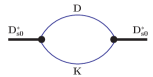
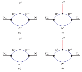
Figure 1: Mass operator of the $D_{s0}^{\ast}(2317)$ meson.

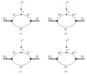
Figure 2: Diagrams contributing to the “direct” strong transition $D_{s0}^{\ast+}\to D_{s}^{+}+\pi^{0}$.

Figure 3: Diagrams contributing to the strong transition $D_{s0}^{\ast+}\to D_{s}^{+}+\pi^{0}$ via $\eta-\pi^{0}$ mixing.

Now we turn to the discussion of the lowest-order diagrams which contribute to the matrix elements of the strong isospin-violating decay $D_{s0}^{\ast}\to D_{s}\pi^{0}$ and the radiative decay $D_{s0}^{\ast}\to D_{s}^{\ast}\gamma$. To the strong decay two types of diagrams contribute: the so-called “direct” diagrams of Fig.2 with $\pi^{0}$-meson emission from the $D^{(\ast)}K$ meson loops and the “indirect” diagrams of Fig.3 where a $\pi^{0}$ meson is produced via $\eta-\pi^{0}$ mixing. Note, that the second mechanism based on $\eta-\pi^{0}$ mixing was mainly considered before in the literature. Originally, it was initiated by the analysis based on the use of chiral Lagrangians Cho:1994zu ; Bardeen:2003kt ; Colangelo:2003vg where the leading-order, tree-level $D_{s0}^{\ast}D_{s}\pi^{0}$ coupling can be generated only by virtual $\eta$-meson emission. During the last years different approaches have been applied to the $D_{s0}^{\ast}\to D_{s}\pi^{0}$ decay properties using the $\eta-\pi^{0}$ mixing mechanism. In our approach the $D_{s0}^{\ast}$ meson is considered as a $DK$ bound state and, therefore, we have an additional mechanism for generating the $D_{s0}^{\ast}D_{s}\pi^{0}$ transition due to the direct coupling of $D^{(\ast)}$ and $K^{(\ast)}$ mesons to $\pi^{0}$. In particular, in the isospin limit (when the masses of the virtual $D^{(\ast)}$ and $K^{(\ast)}$ mesons in the loops are degenerate, respectively) the pairs of diagrams related to Fig.2(a), 2(b) and Fig.2(c) and 2(d) compensate each other. Only the use of physical masses for the $D^{(\ast)}$ and $K^{(\ast)}$ mesons gives a nontrivial contribution to the $D_{s0}^{\ast}\to D_{s}\pi^{0}$ coupling of order $O(\delta)$, where

$$\delta\sim m_{D^{(\ast)\,\pm}}^{2}-m_{D^{(\ast)\,0}}^{2}\sim m_{K^{(\ast)\,\pm}}^{2}-m_{K^{(\ast)\,0}}^{2}$$ (12)

is the parameter of isospin breaking. Therefore, the contribution of the diagrams of Fig.2 is of the same order as the one related to Fig.3 involving $\eta-\pi^{0}$ mixing, where the $\eta-\pi^{0}$ transition coupling (filled black circle) is counted as $O(\delta)$.

The diagrams contributing to the radiative decay $D_{s0}^{\ast\,+}\to D_{s}^{\ast\,+}\gamma$ are shown in Fig.4. The diagrams of Figs.4(a) and 4(b) are generated by the direct coupling of the charged $D^{+}$ and $K^{+}$ mesons to the electromagnetic field after gauging of the free Lagrangians related to these mesons. The diagrams of Figs.4(c) and 4(d) (so-called contact diagrams) are generated after gauging of nonlocal strong Lagrangian (1) describing the coupling of $D_{s0}^{\ast}$ mesons to its constituents - $D$ and $K$ mesons. The diagrams of Figs.4(e) and 4(f) arise after gauging the strong $D^{\ast}_{s}DK$ interaction Lagrangian containing derivatives acting on the pseudoscalar fields. Finally, the diagrams of Figs.4(g) and 4(h) describe the sub-process where the $D_{s0}^{\ast}$ converts into the $D_{s}^{\ast}$ via a $DK$ loop followed by the interaction of the $D_{s}^{\ast}$ with the electromagnetic field. Note that an analogous diagram where the $D_{s}^{\ast}$ meson interacts with the electromagnetic field and then converts into the $D_{s}^{\ast}$ vanishes due to the transversity condition for the on-shell vector meson $D_{s}^{\ast}$, i.e. $p_{\mu}\,\epsilon_{D_{s}^{\ast}}^{\mu}(p)=0$. Details of how to generate the effective couplings of the involved mesons to the electromagnetic field will be discussed later.

After the preliminary discussion of the relevant diagrams, now we are in the position to write down the full effective Lagrangian ${\cal L}_{\rm eff}$ for the study of strong $D_{s0}^{\ast}\to D_{s}\pi^{0}$ and radiative $D_{s0}^{\ast}\to D_{s}^{\ast}\gamma$ decay properties. For convenience we split ${\cal L}_{\rm eff}$ into an isospin-symmetric part ${\cal L}_{\rm inv}$ and an isospin-symmetry breaking part ${\cal L}_{\rm break}$:

$${\cal L}_{\rm eff}(x)\,=\,{\cal L}_{\rm inv}(x)\,+\,{\cal L}_{\rm break}(x)\,,$$ (13)

where ${\cal L}_{\rm inv}$ is given by a sum of free meson parts ${\cal L}_{\rm free}$ and the interaction parts ${\cal L}_{\rm int}$:

$${\cal L}_{\rm inv}(x)\,=\,{\cal L}_{\rm free}(x)\,+\,{\cal L}_{\rm int}(x)\,.$$ (14)

We use the standard free meson Lagrangian involving states with quantum numbers $J^{P}=0^{+},0^{-}$ and $1^{-}$:

$${\cal L}_{\rm free}(x)\,=\,\sum\limits_{i=S,P,V}{\cal L}_{\rm free}^{i}(x)\,,$$ (15)

where

$${\cal L}_{\rm free}^{S}(x) = -D_{s0}^{\ast\,+}(x)(\Box+m_{D_{s0}^{\ast}}^{2})D_{s0}^{\ast\,-}(x)\,,$$ (16)

$${\cal L}_{\rm free}^{P}(x) = -\frac{1}{2}\vec{\pi}(x)(\Box+m_{\pi}^{2})\vec{\pi}(x)-K^{\dagger}(x)(\Box+m_{K}^{2})K(x)-\frac{1}{2}\eta(x)(\Box+m_{\eta}^{2})\eta(x)$$ (17)

$$- D^{\dagger}(x)(\Box+m_{D}^{2})D(x)-D^{+}_{s}(x)(\Box+m_{D_{s}}^{2})D^{-}_{s}(x)\,,$$

$${\cal L}_{\rm free}^{V}(x) = K^{\ast\,\dagger}_{\mu}(x)(g^{\mu\nu}[\Box+m_{K^{\ast}}^{2}]-\partial^{\mu}\partial^{\nu})K^{\ast}_{\nu}(x)+D^{\ast\,\dagger}_{\mu}(x)(g^{\mu\nu}[\Box+m_{D^{\ast}}^{2}]-\partial^{\mu}\partial^{\nu})D^{\ast}_{\nu}(x)$$ (18)

$$+ D^{\ast\,+}_{s\,\mu}(x)(g^{\mu\nu}[\Box+m_{D_{s}^{\ast}}^{2}]-\partial^{\mu}\partial^{\nu})D^{\ast\,-}_{s\,\nu}(x)\,\,.$$

Here $\Box=\partial^{\mu}\partial_{\mu}$, $\vec{\pi}$ is the triplet of pions, $D_{s}^{\pm}$ and $D_{s}^{\ast\,\pm}$ are the pseudoscalar and vector charm-strange mesons, respectively. The doublets of vector mesons $D^{\ast}$ and $K^{\ast}$ are given by

$$D^{\ast}=\left(\begin{array}[]{c}D^{\ast\,0}\\ D^{\ast\,+}\\ \end{array}\right)\,,\hskip 28.45274ptK^{\ast}=\left(\begin{array}[]{c}K^{\ast\,+}\\ K^{\ast\,0}\\ \end{array}\right)\,.$$ (23)

In our convention the isospin-symmetric meson masses of the iso-multiplets are identified with the masses of the charged partners Yao:2006px :

$$m_{\pi}\equiv m_{\pi^{\pm}}=139.57018\ {\rm MeV}\,,\hskip 8.5359ptm_{K}\equiv m_{K^{\pm}}=493.677\ {\rm MeV}\,,\hskip 8.5359ptm_{K^{\ast}}\equiv m_{K^{\ast\,\pm}}=891.66\ {\rm MeV}\,,$$ (24)

$$m_{D}\equiv m_{D^{\pm}}=1.8693\ {\rm GeV}\,,\hskip 21.33955ptm_{D^{\ast}}\equiv m_{D^{\ast\,\pm}}=2.010\ {\rm GeV}\,.$$

The masses of the iso-singlet states are Yao:2006px :

$$m_{\eta}=547.51\ {\rm MeV}\,,\hskip 48.36958ptm_{D_{s}}=m_{D^{\pm}_{s}}=1.9682\ {\rm GeV}\,,$$ (25)

$$m_{D^{\ast}_{s}}=m_{D^{\ast\,\pm}_{s}}=2.112\ {\rm GeV}\,,\hskip 8.5359ptm_{D^{\ast}_{s0}}=m_{D^{\ast\,\pm}_{s0}}=2.3173\ {\rm GeV}\,.$$

The interaction term ${\cal L}_{\rm int}(x)$ will be discussed later. First we would like to write down the isospin-breaking term ${\cal L}_{\rm break}$, which includes the mass corrections of the neutral mesons containing $u$ or $d$ quarks and the $\eta-\pi^{0}$ mass mixing Gross:1979ur ; Cho:1994zu :

$${\cal L}_{\rm break}(x)\,=\,\delta{\cal L}^{P}(x)+\delta{\cal L}^{V}(x)+{\cal L}_{\eta\pi}(x)\,,$$ (26)

where

$$\delta{\cal L}^{P}(x) = \frac{\delta_{\pi}}{2}\,[\pi^{0}(x)]^{2}+\delta_{K}\,\bar{K}^{0}(x)K^{0}(x)+\delta_{D}\,\bar{D}^{0}(x)D^{0}(x)\,,$$ (27)

$$\delta{\cal L}^{V}(x) = -\delta_{K^{\ast}}\,\bar{K}^{\ast\,0}_{\mu}(x)K^{\ast\,0\,\mu}(x)-\delta_{D^{\ast}}\,\bar{D}^{\ast\,0}_{\mu}(x)D^{\ast\,0\,\mu}(x)\,,$$ (28)

$${\cal L}_{\eta\pi}(x) = B\,\frac{m_{d}-m_{u}}{\sqrt{3}}\,\pi^{0}(x)\,\eta(x)\,,$$ (29)

where $m_{u}$ and $m_{d}$ are the $u$ and $d$ current quark masses, $B$ is the condensate parameter. Here $\delta_{M}$ are the isospin-breaking parameters which are fixed by the difference of masses squared of the charged and neutral members of the iso-multiplets as:

$$\delta_{M}=m_{M^{\pm}}^{2}-m_{M^{0}}^{2}\,,\hskip 14.22636ptm_{M^{0}}\equiv m_{\bar{M}^{0}}\,.$$ (30)

The set of $m_{M^{0}}$ is taken from data Yao:2006px with:

$$m_{\pi^{0}}=134.9766\ {\rm MeV}\,,\hskip 8.5359ptm_{K^{0}}=497.648\ {\rm MeV}\,,\hskip 8.5359ptm_{K^{\ast\,0}}=896.0\ {\rm MeV}\,,$$ (31)

$$m_{D^{0}}=1.8645\ {\rm GeV}\,,\hskip 8.5359pt\hskip 8.5359ptm_{D^{\ast\,0}}=2.0067\ {\rm GeV}\,.$$

Eqs. (16)-(18), (27) and (28) define the free meson propagators for scalar (pseudoscalar) fields

$$i\,D_{M}(x-y)=\langle 0|T\,M(x)\,M^{\dagger}(y)|0\rangle\ =\ \int\frac{d^{4}k}{(2\pi)^{4}i}\,e^{-ik(x-y)}\ \tilde{D}_{M}(k)\,,$$ (32)

where

$$\tilde{D}_{M}(k)=\frac{1}{m_{M}^{2}-k^{2}-i\epsilon}$$ (33)

and vector fields

$$i\,D_{M^{\ast}}^{\mu\nu}(x-y)=\langle 0|T\,M^{\ast\,\mu}(x)\,M^{\ast\,\nu\,\dagger}(y)|0\rangle\ =\ \int\frac{d^{4}k}{(2\pi)^{4}i}\,e^{-ik(x-y)}\ \tilde{D}_{M^{\ast}}^{\mu\nu}(k)$$ (34)

where

$$\tilde{D}_{M^{\ast}}^{\mu\nu}(k)=-\frac{1}{m_{M^{\ast}}^{2}-k^{2}-i\epsilon}\biggl{(}g^{\mu\nu}-\frac{k^{\mu}k^{\nu}}{m_{M^{\ast}}^{2}}\biggr{)}\,.$$ (35)

In the following calculations it will be convenient to expand the propagators of the neutral mesons $D^{0}(\bar{D}^{0})$, $K^{0}(\bar{K}^{0})$, $D^{\ast\,0}(\bar{D}^{\ast\,0})$ and $K^{\ast\,0}(\bar{K}^{\ast\,0})$ in powers of the corresponding isospin-breaking parameters as:

$$\tilde{D}_{M^{0}}(k) = \biggl{[}1-\delta_{M}\frac{\partial}{\partial m_{M^{\pm}}^{2}}\biggr{]}\tilde{D}_{M^{\pm}}(k)+O(\delta_{M}^{2})\,,$$ (36)

$$\tilde{D}_{M^{\ast\,0}}^{\mu\nu}(k) = \biggl{[}1-\delta_{M^{\ast}}\frac{\partial}{\partial m_{M^{\ast\pm}}^{2}}\biggr{]}\tilde{D}_{M^{\ast\,\pm}}^{\mu\nu}(k)+O(\delta_{M^{\ast}}^{2})\,.$$

The interaction Lagrangian includes the strong and electromagnetic parts

$${\cal L}_{\rm int}(x)={\cal L}_{\rm int}^{\rm str}(x)+{\cal L}_{\rm int}^{\rm em}(x)\,,$$ (37)

as already apparent from the previous discussion related to Figs.2-4. The relevant strong part of the effective Lagrangian contains the following terms: the Lagrangian ${\cal L}_{D_{s0}^{\ast}}$ (1) describing the coupling of the $D_{s0}^{\ast}$ meson to its constituents and $VPP$-type Langrangians, describing the interaction of vector mesons with two pseudoscalars:

$${\cal L}_{\rm int}^{\rm str}(x) = {\cal L}_{D_{s0}^{\ast}}(x)+{\cal L}_{D^{\ast}D\pi}(x)+{\cal L}_{D^{\ast}D\eta}(x)+{\cal L}_{K^{\ast}K\pi}(x)+{\cal L}_{K^{\ast}K\eta}(x)$$ (38)

$$+ {\cal L}_{D^{\ast}D_{s}K}(x)+{\cal L}_{K^{\ast}D_{s}D}(x)+{\cal L}_{D^{\ast}_{s}DK}(x)\,.$$

Let us specify the $VPP$ interaction Lagrangians occurring in Eqs. (38). In general they can be defined as:

$${\cal L}_{VP_{1}P_{2}}(x)\,=\,g_{{}_{VP_{1}P_{2}}}\,V_{\mu}(x)\,P_{1}(x)\,i\!\stackrel{{\scriptstyle\leftrightarrow}}{{\partial}}^{\,\mu}P_{2}(x)\,+\,{\rm H.c.}$$ (39)

To be consistent with the definitions occurring in literature, we use the following form of the particular Lagrangians:

$${\cal L}_{D^{\ast}D\pi}(x) = -\frac{g_{{}_{D^{\ast}D\pi}}}{2\sqrt{2}}\,D^{\ast\,\dagger}_{\mu}(x)\,\vec{\tau}\,\vec{\pi}(x)i\!\stackrel{{\scriptstyle\leftrightarrow}}{{\partial}}^{\,\mu}\!D(x)\,+\,{\rm H.c.}\,$$ (40)

$${\cal L}_{D^{\ast}D\eta}(x) = -\frac{g_{{}_{D^{\ast}D\eta}}}{2\sqrt{2}}\,D^{\ast\,\dagger}_{\mu}(x)\,\eta(x)\,i\!\stackrel{{\scriptstyle\leftrightarrow}}{{\partial}}^{\,\mu}\!D(x)\,+\,{\rm H.c.}\,$$ (41)

$${\cal L}_{K^{\ast}K\pi}(x) = \frac{g_{{}_{K^{\ast}K\pi}}}{\sqrt{2}}\,K^{\ast\,\dagger}_{\mu}(x)\,\vec{\tau}\,\vec{\pi}(x)i\!\stackrel{{\scriptstyle\leftrightarrow}}{{\partial}}^{\,\mu}\!K(x)\,+\,{\rm H.c.}\,$$ (42)

$${\cal L}_{K^{\ast}K\eta}(x) = \frac{g_{{}_{K^{\ast}K\eta}}}{\sqrt{2}}\,K^{\ast\,\dagger}_{\mu}(x)\,\eta(x)\,i\!\stackrel{{\scriptstyle\leftrightarrow}}{{\partial}}^{\,\mu}\!K(x)\,+\,{\rm H.c.}\,$$ (43)

$${\cal L}_{D^{\ast}D_{s}K}(x) = g_{{}_{D^{\ast}D_{s}K}}\,D^{\ast\,T}_{\mu}(x)\,K(x)\,i\!\stackrel{{\scriptstyle\leftrightarrow}}{{\partial}}^{\,\mu}\!D_{s}^{-}(x)\,+\,{\rm H.c.}\,$$ (44)

$${\cal L}_{K^{\ast}D_{s}D}(x) = g_{{}_{K^{\ast}D_{s}D}}\,K^{\ast\,T}_{\mu}(x)D(x)\,i\!\stackrel{{\scriptstyle\leftrightarrow}}{{\partial}}^{\,\mu}\!D_{s}^{-}(x)\,\,+\,{\rm H.c.}\,$$ (45)

$${\cal L}_{D^{\ast}_{s}DK}(x) = g_{{}_{D^{\ast}_{s}DK}}\,D^{\ast\,-}_{s\,\mu}(x)\,D^{T}(x)\,i\!\stackrel{{\scriptstyle\leftrightarrow}}{{\partial}}^{\,\mu}\!K(x)\,+\,{\rm H.c.}\,$$ (46)

where summation over isospin indices is understood and $A\stackrel{{\scriptstyle\leftrightarrow}}{{\partial}}B\equiv A\partial B-B\partial A$.

The couplings $g_{{}_{D^{\ast}D\pi}}$ and $g_{{}_{K^{\ast}K\pi}}$ are fixed by data for the strong decay widths $D^{\ast}\to D\pi$ and $K^{\ast}\to K\pi$. In particular, the strong two-body decay widths $\Gamma(D^{\ast\,+}\to D^{0}\pi^{+})$ and $\Gamma(K^{\ast\,+}\to K^{0}\pi^{+})$ are related to $g_{{}_{D^{\ast}D\pi}}$ Belyaev:1994zk ; Anastassov:2001cw and $g_{{}_{K^{\ast}K\pi}}$ as

$$\Gamma(D^{\ast\,+}\to D^{0}\pi^{+}) = \frac{g_{{}_{D^{\ast}D\pi}}^{2}}{24\pi m_{D^{\star+}}^{2}}\,P_{{}_{\pi D^{\ast}}}^{3}\,,$$ (47)

$$\Gamma(K^{\ast\,+}\to K^{0}\pi^{+}) = \frac{g_{{}_{K^{\ast}K\pi}}^{2}}{6\pi m_{K^{\star+}}^{2}}\,P_{{}_{\pi K^{\ast}}}^{3}\,,$$ (48)

where $P_{{}_{\pi V}}$ is the three-momentum of $\pi^{+}$ in the rest frame of the decaying vector meson $V$. Using data for the corresponding strong decay widths one deduces: $g_{{}_{D^{\ast}D\pi}}=17.9$ Anastassov:2001cw and $g_{{}_{K^{\ast}K\pi}}=4.61$ Yao:2006px .

The coupling constants $g_{{}_{D^{\ast}D\pi(\eta)}}$ are obtained in the context of heavy hadron chiral perturbation theory (HHChPT) Wise:1992hn . The couplings $g_{{}_{D^{\ast}D\pi}}$ and $g_{{}_{D^{\ast}D\eta}}$ are expressed (and then related) in terms of a universal strong coupling constant $g$ involving heavy (vector and pseudoscalar) and Goldstone mesons and in terms of the leptonic decay constants $F_{P}$:

$$g_{{}_{D^{\ast}D\pi}}=\frac{m_{D^{\ast}}}{F_{\pi}}g\,\sqrt{2}\,,\hskip 8.5359ptg_{{}_{D^{\ast}D\eta}}=\frac{m_{D^{\ast}}}{F_{\eta}}g\,\sqrt{\frac{2}{3}}\,,$$ (49)

where $F_{\pi}=92.4$ MeV and $F_{\eta}=1.3\,F_{\pi}$. From Eq. (49) and using $g_{{}_{D^{\ast}D\pi}}=17.9$ we deduce the value of $g_{{}_{D^{\ast}D\eta}}$ with

$$g_{{}_{D^{\ast}D\eta}}\,=\,\frac{F_{\pi}}{F_{\eta}\sqrt{3}}g_{{}_{D^{\ast}D\pi}}\,=\,7.95\,.$$ (50)

The coupling constant $g_{{}_{K^{\ast}K\eta}}$ can be related to $g_{{}_{K^{\ast}K\pi}}$ using the unitary symmetry relation:

$$g_{{}_{K^{\ast}K\eta}}\,=\,\frac{F_{\pi}\sqrt{3}}{F_{\eta}}g_{{}_{K^{\ast}K\pi}}\,=\,6.14\,.$$ (51)

Again, as in the case of $g_{{}_{D^{\ast}D\pi(\eta)}}$, we include in couplings the relation to the corresponding decay constants $F_{\pi}$ and $F_{\eta}$.

The coupling constants $g_{{}_{D^{\ast}D_{s}K}}$ and $g_{{}_{D_{s}^{\ast}DK}}$ have been estimated using the QCD sum rule technique in Refs. Wang:2006id ; Bracco:2006xf . These couplings are important for the evaluation of the dissociation cross section of $J/\Psi$ to kaons (see, e.g. discussion in Refs. Haglin:1999xs ; Azevedo:2003qh .). Here we use the results of Ref. Wang:2006id : $g_{{}_{D^{\ast}D_{s}K}}=2.02$ and $g_{{}_{D_{s}^{\ast}DK}}=1.84$. The coupling $g_{{}_{K^{\ast}D_{s}D}}$ can also be related to $g_{{}_{D^{\ast}D_{s}K}}$, using $SU(4)$ symmetry arguments: $g_{{}_{K^{\ast}D_{s}D}}=g_{{}_{D^{\ast}D_{s}K}}=2.02$.

The relevant electromagnetic part has three main terms:

$${\cal L}_{\rm int}^{\rm em}(x)={\cal L}_{\rm int}^{\rm em(1)}(x)+{\cal L}_{\rm int}^{\rm em(2)}(x)+{\cal L}_{\rm int}^{\rm em(3)}(x)\,.$$ (52)

The first term describes the local coupling of charged $D$-, $K$- and $D_{s}^{\ast}$ mesons to the electromagnetic field

$${\cal L}^{\rm em(1)}_{\rm int}(x) = ieA_{\mu}(x)\,\biggl{\{}\,D^{-}(x)\stackrel{{\scriptstyle\leftrightarrow}}{{\partial}}^{\,\mu}\!D^{+}(x)+K^{-}(x)\stackrel{{\scriptstyle\leftrightarrow}}{{\partial}}^{\,\mu}\!K^{+}(x)\,$$ (53)

$$- D_{s}^{\ast-\alpha}(x)\stackrel{{\scriptstyle\leftrightarrow}}{{\partial}}^{\,\mu}\!D_{s\alpha}^{\ast+}(x)+\frac{1}{2}D_{s}^{\ast-\alpha}(x)\stackrel{{\scriptstyle\leftrightarrow}}{{\partial}}_{\,\alpha}\!D_{s}^{\ast+\mu}(x)+\frac{1}{2}D_{s}^{\ast-\mu}(x)\stackrel{{\scriptstyle\leftrightarrow}}{{\partial}}^{\,\alpha}\!D_{s\alpha}^{\ast+}(x)\biggr{\}}\,.$$

The term ${\cal L}^{\rm em(1)}_{\rm int}$ is generated after gauging of the free meson Lagrangians using minimal substitution:

$$\partial^{\mu}M^{\pm}\,\to\,(\partial^{\mu}\mp ieA^{\mu})\,M^{\pm}\,.$$ (54)

The terms ${\cal L}_{\rm int}^{\rm em(2)}$ and ${\cal L}_{\rm int}^{\rm em(3)}$ are generated due to the gauging of the strong Lagrangians (39) and (1) containing derivatives acting on the charged fields. Note, that the correlation function $\Phi_{D_{s0}^{\ast}}$, describing the nonlocal $D_{s0}^{\ast}DK$ coupling, is a function of $\partial^{2}$ and, therefore, both Lagrangians (39) and (1) are not gauge-invariant under electromagnetic $U_{\rm em}(1)$ transformations and should be modified accordingly.

To get the second term we replace all derivatives acting on the charged fields by the covariant ones using minimal substitution (as is the case for gauging the free Lagrangians). The term in ${\cal L}^{\rm em(2)}$ relevant for our calculation in contains the coupling of the vector $D_{s}^{\ast}$ meson to $D$, $K$ and the photon field with

$${\cal L}^{\rm em(2)}_{\rm int}(x) = e\,g_{{}_{D^{\ast}_{s}DK}}\,A^{\mu}(x)\,D^{\ast\,-}_{s\,\mu}(x)\,[\,D^{0}(x)\,K^{+}(x)\,-\,D^{+}(x)\,K^{0}(x)\,]\,+\,{\rm H.c.}\,+\,\cdots$$ (55)

The gauging of the nonlocal Lagrangian of Eq. (1) proceeds in a way suggested in Ref. Mandelstam:1962mi and extensively used in Refs. Efimov:1987na ; Faessler:2003yf . In particular, to guarantee local invariance of the strong interaction Lagrangian, in ${\cal L}_{\rm int}^{\rm str}$ each charged constituent meson field (i.e. $D^{\pm}$ and $K^{\pm}$ meson fields) are multiplied by the gauge field exponential resulting in

$${\cal L}_{\rm int}^{\rm str+em(3)}(x) = g_{{}_{D_{s0}^{\ast}}}\,D_{s0}^{\ast\,-}(x)\,\int\!dy\,\Phi_{D_{s0}^{\ast}}(y^{2})\,\biggl{\{}e^{-ieI(x+w_{K}y,x,P)}D^{+}(x+w_{K}y)K^{0}(x-w_{D}y)\,$$ (56)

$$+ D^{0}(x+w_{K}y)e^{-ieI(x-w_{D}y,x,P)}K^{+}(x-w_{D}y)\biggr{\}}\,+\,{\rm H.c.}$$

where

$$I(x,y,P)=\int\limits_{y}^{x}dz_{\mu}A^{\mu}(z).$$ (57)

For the derivative of the path integral (57) we use the path-independent prescription suggested in Refs. Mandelstam:1962mi

$$\lim\limits_{dx^{\mu}\to 0}dx^{\mu}\frac{\partial}{\partial x^{\mu}}I(x,y,P)\,=\,\lim\limits_{dx^{\mu}\to 0}[I(x+dx,y,P^{\prime})-I(x,y,P)]\,,$$ (58)

where path $P^{\prime}$ is obtained from $P$ when shifting the end-point $x$ by $dx$. Use of the definition (58) leads to the key rule

$$\frac{\partial}{\partial x^{\mu}}I(x,y,P)=A_{\mu}(x)\,,$$ (59)

which in turn states that the derivative of the path integral $I(x,y,P)$ does not depend on the path P originally used in the definition. The non-minimal substitution (56) is therefore completely equivalent to the minimal prescription.

In the calculation of the amplitudes of the radiative $D_{s0}^{\ast}\to D_{s}^{\ast}\gamma$ decay, in Eq. (56) we only need to keep terms linear in $A_{\mu}$, that is the four-particle coupling $D_{s0}^{\ast}DK\gamma$. Hence, the third term contributing to the electromagnetic interaction Lagrangian is given by

$${\cal L}_{\rm int}^{\rm em(3)}(x) = -\,ieg_{{}_{D_{s0}^{\ast}}}\,D_{s0}^{\ast\,-}(x)\,\int\!dy\,\Phi_{D_{s0}^{\ast}}(y^{2})\,\biggl{\{}\int\limits_{x}^{x+w_{K}y}dz_{\mu}A^{\mu}(z)D^{+}(x+w_{K}y)K^{0}(x-w_{D}y)\,$$

$$+ \int\limits_{x}^{x-w_{D}y}dz_{\mu}A^{\mu}(z)D^{0}(x+w_{K}y)K^{+}(x-w_{D}y)\biggr{\}}\,+\,{\rm H.c.}+\cdots$$

Concluding the discussion of the effective interaction Lagrangian we stress that all couplings occurring in the diagrams contributing to the decays $D_{s0}^{\ast}\to D_{s}\pi^{0}$ and $D_{s0}^{\ast}\to D_{s}^{\ast}\gamma$ are explicitly fixed, except $g_{{}_{D_{s0}^{\ast}}}$ discussed in the following.

II.3 Analysis of the $D_{s0}^{\ast}DK$ coupling $g_{{}_{D_{s0}^{\ast}}}$

Finally, we discuss the numerical value of the model-dependent constant $g_{{}_{D_{s0}^{\ast}}}$. In terms of a general functional form of the correlation function ${\widetilde{\Phi}}_{D_{s0}^{\ast}}$ the coupling constant $g_{{}_{D_{s0}^{\ast}}}$ is given by:

$$\frac{1}{g_{{}_{D_{s0}^{\ast}}}^{2}}=\frac{2}{(4\pi\Lambda_{D_{s0}^{\ast}})^{2}}\,\int\limits_{0}^{\infty}\int\limits_{0}^{\infty}\frac{R\,d\alpha_{1}d\alpha_{2}}{(1+\alpha_{1}+\alpha_{2})^{3}}\,\,[-d\tilde{\Phi}^{2}_{D_{s0}^{\ast}}(z)/dz]\,,$$ (61)

where

$$z = \mu_{D}^{2}\alpha_{1}+\mu_{K}^{2}\alpha_{2}-\frac{R\,\mu_{D_{s0}^{\ast}}^{2}}{1+\alpha_{1}+\alpha_{2}}\,,$$ (62)

$$R = \alpha_{1}\alpha_{2}+\alpha_{1}w_{D}^{2}+\alpha_{2}w_{K}^{2}\,,\hskip 14.22636pt\mu_{M}=\frac{m_{M}}{\Lambda_{D_{s0}^{\ast}}}\,.$$

One should stress that coupling constant $g_{{}_{D_{s0}^{\ast}}}$ remains finite when we remove the cutoff $\Lambda_{D_{s0}^{\ast}}\to\infty$ (local limit). A finite result is obtained, because the derivative of the $D_{s0}^{\ast}$ mass operator is convergent, i.e. the loop integral is $\int d^{4}k/k^{6}$ when the correlation function $\tilde{\Phi}_{D_{s0}^{\ast}}$ is removed (or equal to one) at $\Lambda_{D_{s0}^{\ast}}\to\infty$. However, in the calculation of transition diagrams (like in Figs.2-4) we deal with divergent integral and, therefore, we need the correlation function to perform the regularization of the occurring loop integrals. Now the question is how sensitive our results are to a variation of $\Lambda_{D_{s0}^{\ast}}$. First, we look at the coupling constant $g_{{}_{D_{s0}^{\ast}}}$. In the limit $\Lambda_{D_{s0}^{\ast}}\to\infty$ it is given by

$$\frac{1}{g_{{}_{D_{s0}^{\ast}}}^{2}}=\frac{2}{(4\pi m_{D_{s0}^{\ast}})^{2}}\,\biggl{\{}\frac{m_{D}^{2}-m_{K}^{2}}{m_{D_{s0}^{\ast}}^{2}}\,{\rm ln}\frac{m_{D}}{m_{K}}\,-1\,+\,\frac{m_{D_{s0}^{\ast}}^{2}(m_{D}^{2}+m_{K}^{2})-(m_{D}^{2}-m_{K}^{2})^{2}}{m_{D_{s0}^{\ast}}^{2}\sqrt{-\lambda}}\,\sum\limits_{\pm}{\rm arctan}\frac{z_{\pm}}{\sqrt{-\lambda}}\biggr{\}}$$ (63)

where $z_{\pm}=m_{D_{s0}^{\ast}}^{2}\pm(m_{D}^{2}-m_{K}^{2})$ and

$$\lambda\doteq\lambda(m_{D_{s0}^{\ast}}^{2},m_{D}^{2},m_{K}^{2})=m_{D_{s0}^{\ast}}^{4}+m_{D}^{4}+m_{K}^{4}-2m_{D_{s0}^{\ast}}^{2}m_{D}^{2}-2m_{D_{s0}^{\ast}}^{2}m_{K}^{2}-2m_{D}^{2}m_{K}^{2}$$ (64)

is the Källen function.

For checking purposes we also analyze the coupling $g_{{}_{D_{s0}^{\ast}}}$ in the heavy quark limit (HQL), where the masses of $D$ and $D_{s0}^{\ast}$ mesons together with the charm quark mass $m_{c}$ go to infinity. In the HQL the $D$ meson in the $D_{s0}^{\ast}$ molecule fixes the center-of-mass, surrounded by a light $K$ meson in analogy to the heavy-light $Q\bar{q}$ mesons. For the nonlocal case the result for $g_{{}_{D_{s0}^{\ast}}}$ in the HQL is:

$$\frac{1}{g_{{}_{D_{s0}^{\ast}}}^{2}} = \frac{1}{(4\pi m_{c})^{2}}\,\int\limits_{0}^{\infty}\frac{\displaystyle{d\alpha}}{\displaystyle{1+\mu_{K}^{2}\alpha}}\,\,\Phi^{2}_{D_{s0}^{\ast}}(\alpha)\,.$$ (65)

The HQL result for the local case is:

$$\frac{1}{g_{{}_{D_{s0}^{\ast}}}^{2}}=\frac{1}{(4\pi m_{c})^{2}}\,{\rm ln}\frac{m_{c}^{2}}{m_{K}^{2}}\,.$$ (66)

Now we compare our numerical results for the coupling constant $g_{{}_{D_{s0}^{\ast}}}$ in different regimes: 1) nonlocal case (NC); 2) local case (LC); 3) nonlocal case + HQL (NCHQL) and 4) local case + HQL (LCHQL). When we deal with the nonlocal case we proceed with the Gaussian correlation function $\Phi_{D_{s0}^{\ast}}(z)={\rm exp}(-z)$ and vary the scale parameter $\Lambda_{D_{s0}^{\ast}}$ from 1 to 2 GeV. For the charm quark mass we use the averaged result of the PDG Yao:2006px : $m_{c}=1.25$ GeV. For a convenience we attach a corresponding superscript to $g_{{}_{D_{s0}^{\ast}}}$ to indicate the specific regime.

We get the following results: the coupling $g_{{}_{D_{s0}^{\ast}}}^{\rm NC}$ varies from 11.26 GeV at $\Lambda_{D_{s0}^{\ast}}=1$ GeV to 9.90 GeV at $\Lambda_{D_{s0}^{\ast}}=2$ GeV. The coupling $g_{{}_{D_{s0}^{\ast}}}^{\rm LC}$ is expressed only in terms of physical meson masses with the result $g_{{}_{D_{s0}^{\ast}}}^{\rm LC}=8.98$ GeV. The coupling $g_{{}_{D_{s0}^{\ast}}}^{\rm NCHQL}$ varies from 16.22 GeV at $\Lambda_{D_{s0}^{\ast}}=1$ GeV to 11.52 GeV at $\Lambda_{D_{s0}^{\ast}}=2$ GeV. Finally, we have $g_{{}_{D_{s0}^{\ast}}}^{\rm LCHQL}=11.52$ GeV. All results for $g_{{}_{D_{s0}^{\ast}}}$ are quite close to each other with a typical value for $g_{{}_{D_{s0}^{\ast}}}$ of about 10 GeV which is consistent with preceding calculations done in other theoretical approaches. In Table 1 we compare our result for the $D_{s0}^{\ast}DK$ coupling constant to predictions of other theoretical approaches (we use a compilation of the results done in Ref. Wang:2006id ).

II.4 Extension to other possible hadronic molecules

We end this section with a comment concerning the extension of the derived framework to the study of other hadronic molecules. This can be done in a straightforward fashion. The starting point is the construction of an effective Lagrangian describing hadronic molecules as bound states of its constituents. In particular, for the case of the charm-strange meson $D_{s1}(2460)$ and for the possible partners in the bottom sector $B_{s0}^{\ast}(5725)$ and $B_{s1}(5778)$ the simplest Lagrangians have the form:

$${\cal L}_{D_{s1}}(x) = g_{{}_{D_{s1}}}\,D_{s1}^{-\,\mu}(x)\,\int\!dy\,\Phi_{D_{s1}}(y^{2})\,D^{\ast\,T}_{\mu}(x+w_{{}_{KD^{\ast}}}y)\,K(x-w_{{}_{D^{\ast}K}}y)\,+\,{\rm H.c.}\,,$$ (67)

$${\cal L}_{B_{s0}^{\ast}}(x) = g_{{}_{B_{s0}^{\ast}}}\,\bar{B}_{s0}^{\ast\,0}(x)\,\int\!dy\,\Phi_{B_{s0}^{\ast}}(y^{2})\,B^{\dagger}(x+w_{{}_{KB}}y)\,K(x-w_{{}_{BK}}y)\,+\,{\rm H.c.}\,,$$ (68)

$${\cal L}_{B_{s1}}(x) = g_{{}_{B_{s1}}}\,\bar{B}_{s1}^{0\,\mu}(x)\,\int\!dy\,\Phi_{B_{s1}}(y^{2})\,B^{\ast\,\dagger}_{\mu}(x+w_{{}_{KB^{\ast}}}y)\,K(x-w_{{}_{B^{\ast}K}}y)\,+\,{\rm H.c.}\,,$$ (69)

where $w_{ij}=m_{i}/(m_{i}+m_{j})$, $g_{M}$ and $\Phi_{M}$ are the coupling constants (fixed from the compositeness condition) and correlation functions. The doublets of $B^{(\ast)}$ and $B^{(\ast)\,\dagger}$ mesons are defined as

$$B^{(\ast)}=\left(\begin{array}[]{c}B^{(\ast)\,+}\\ B^{(\ast)\,0}\\ \end{array}\right)\,,\hskip 28.45274ptB^{(\ast)\,\dagger}=(B^{(\ast)\,-}\ \ \bar{B}^{(\ast)\,0})\,.$$ (72)

The molecular structure of $D_{s1}^{\pm}$, $B_{s0}^{\ast\,0}$, $\bar{B}_{s0}^{\ast\,0}$, $B_{s1}^{0}$ and $\bar{B}_{s1}^{0}$ is:

$$|D_{s1}^{+}\rangle\,=\,|D^{\ast\,+}K^{0}\rangle+|D^{\ast\,0}K^{+}\rangle\,,\hskip 28.45274pt|D_{s1}^{-}\rangle\,=\,|D^{\ast\,-}\bar{K}^{0}\rangle+|\bar{D}^{\ast\,0}K^{-}\rangle\,,$$

$$|B_{s0}^{\ast 0}\rangle\,=\,|B^{+}K^{-}\rangle+|B^{0}\bar{K}^{0}\rangle\,,\hskip 39.83368pt|\bar{B}_{s0}^{\ast 0}\rangle\,=\,|B^{-}K^{+}\rangle+|\bar{B}^{0}K^{0}\rangle\,$$ (73)

$$|B_{s1}^{0}\rangle\,=\,|B^{\ast\,+}K^{-}\rangle+|B^{\ast\,0}\bar{K}^{0}\rangle\,,\hskip 29.87547pt|\bar{B}_{s1}^{0}\rangle\,=\,|B^{\ast\,-}K^{+}\rangle+|\bar{B}^{\ast 0}K^{0}\rangle\,.$$

The calculation of decay properties of $D_{s1}(2460)$, $B_{s0}^{\ast}(5725)$ and $B_{s1}(5778)$ mesons goes beyond the scope of the present paper and we relegate this issue to a forthcoming paper.

III Strong $D_{s0}^{\ast}\to D_{s}\pi^{0}$ and radiative $D_{s0}^{\ast}\to D_{s}^{\ast}\gamma$ decays

In this section we discuss the numerical results for the $D_{s0}^{\ast}\to D_{s}\pi^{0}$ and $D_{s0}^{\ast}\to D_{s}^{\ast}\gamma$ decay properties. As we already stressed in the preceding section two types of diagrams contribute to the amplitude of the strong decay $D_{s0}^{\ast}\to D_{s}\pi^{0}$: the “direct” diagrams of Fig.2 and the “$\eta-\pi^{0}$ mixing” diagrams of Fig.3. The “direct” diagrams occur due to the $DK$ molecular structure of the $D_{s0}^{\ast}$ meson, while in the two-quark picture they are forbidden according to the Okubo-Zweig-Iizuka rule. In the framework of our approach this is not the case, since $D$ and $K$ mesons contain nonstrange quarks. The total contribution of the “direct” diagrams starts at order $O(\delta)$, where $\delta$ of Eq. (12) is the generic parameter of isospin breaking. Hence, the “direct diagrams” are of the same order in the isospin-breaking counting scheme as the “$\eta-\pi^{0}$ mixing” diagrams, and, therefore, both types of diagrams should be included. To clarify this mechanism we present our results our results for two cases: 1) “full calculation” (Full) and 2) “leading-order” (LO), i.e. restricting to first order in isospin-breaking $O(\delta)$.

It is convenient to write the matrix element describing the $D_{s0}^{\ast}\to D_{s}\pi^{0}$ transition as a sum of the added contributions of the diagrams in Figs.2 and 3:

$$M(D_{s0}^{\ast}\to D_{s}\pi^{0})\,=\,M_{\rm dir}(D_{s0}^{\ast}\to D_{s}\pi^{0})\,+\,M_{\rm mix}(D_{s0}^{\ast}\to D_{s}\pi^{0})$$ (74)

with

$$M_{\rm dir}(D_{s0}^{\ast}\to D_{s}\pi^{0})=g_{D_{s0}^{\ast}D_{s}\pi^{0}}\,,$$ (75)

$$M_{\rm mix}(D_{s0}^{\ast}\to D_{s}\pi^{0})=g_{D_{s0}^{\ast}D_{s}\eta}\frac{m_{d}-m_{u}}{m_{s}-\hat{m}}\frac{\sqrt{3}}{4}\,,$$ (76)

where $\hat{m}=(m_{u}+m_{d})/2$ and $(m_{d}-m_{u})/(m_{s}-\hat{m})=1/43.7$ (see e.g. Ref. Cho:1994zu ). In the derivation of Eq. (76) we use the masses of $\pi^{0}$ and $\eta$ meson in leading order of the chiral expansion. The total effective $D_{s0}^{\ast}D_{s}\pi^{0}$ coupling, denoted as $G_{D_{s0}^{\ast}D_{s}\pi}$ includes both contributions of the set of diagrams of Figs.2 and 3 with

$$G_{D_{s0}^{\ast}D_{s}\pi}\,=\,G_{D_{s0}^{\ast}D_{s}\pi}^{\rm dir}+G_{D_{s0}^{\ast}D_{s}\pi}^{\rm mix}\,,$$ (77)

$$G_{D_{s0}^{\ast}D_{s}\pi}^{\rm dir}\equiv g_{D_{s0}^{\ast}D_{s}\pi}\,,\hskip 14.22636ptG_{D_{s0}^{\ast}D_{s}\pi}^{\rm mix}\equiv g_{D_{s0}^{\ast}D_{s}\eta}\frac{m_{d}-m_{u}}{m_{s}-\hat{m}}\frac{\sqrt{3}}{4}\,.$$ (78)

In terms of $G_{D_{s0}^{\ast}D_{s}\eta}$ the $D_{s0}^{\ast}\to D_{s}\pi^{0}$ decay width reads as:

$$\Gamma(D_{s0}^{\ast}\to D_{s}\pi)\,=\,\frac{G_{D_{s0}^{\ast}D_{s}\pi}^{2}}{8\pi m_{D_{s0}^{\ast}}^{2}}\,P^{\ast}_{\pi^{0}}\,,$$ (79)

where $P^{\ast}_{\pi^{0}}=\lambda^{1/2}(m_{D_{s0}^{\ast}}^{2},m_{D_{s}}^{2},m_{\pi^{0}}^{2})/(2m_{D_{s0}^{\ast}})$ is the three-momentum of the decay products.

The matrix element describing the $D_{s0}^{\ast}\to D_{s}^{\ast}\gamma$ transition can be written in the manifestly gauge-invariant form

$$M_{\mu\nu}(D_{s0}^{\ast}\to D_{s}^{\ast}\gamma)\,=\,e\,G_{D_{s0}^{\ast}D_{s}^{\ast}\gamma}\,(g_{\mu\nu}p^{\prime}q-p^{\prime}_{\mu}q_{\nu})\,,$$ (80)

where $p^{\prime}$ and $q$ are the $D_{s}^{\ast}$ and photon four-momenta and $p=p^{\prime}+q$ is the $D_{s0}^{\ast}$ momentum. Here $G_{D_{s0}^{\ast}D_{s}^{\ast}\gamma}$ is the effective $D_{s0}^{\ast}D_{s}^{\ast}\gamma$ coupling constant and the $D_{s0}^{\ast}\to D_{s}^{\ast}\gamma$ decay width is given by

$$\Gamma(D_{s0}^{\ast}\to D_{s}^{\ast}\gamma)\,=\,\alpha\,G_{D_{s0}^{\ast}D_{s}^{\ast}\gamma}^{2}\,P_{\gamma}^{\ast\,3}$$ (81)

where

$$P^{\ast}_{\gamma}\,=\,\frac{m_{D_{s0}^{\ast}}}{2}\,\biggl{[}1-\frac{m_{D_{s}^{\ast}}^{2}}{m_{D_{s0}^{\ast}}^{2}}\biggr{]}$$ (82)

is the three-momentum of the decay products.

Now we present the numerical results. First we discuss the contributions of the different diagrams of Figs.2 and 3 to the effective coupling $G_{D_{s0}^{\ast}D_{s}\pi}$. With a typical value for the scale parameter of $\Lambda_{D_{s0}^{\ast}}=1$ GeV we get the following.

In the Full calculation,

$$G_{D_{s0}^{\ast}D_{s}\pi}=146.6\ {\rm MeV}\,,\hskip 8.5359ptG_{D_{s0}^{\ast}D_{s}\pi}^{\rm dir}=104.5\ {\rm MeV}\,,\hskip 8.5359ptG_{D_{s0}^{\ast}D_{s}\pi}^{\rm mix}=42.1\ {\rm MeV}\,,$$ (83)

$$G_{D_{s0}^{\ast}D_{s}\pi}^{DD^{\ast}K}=40.9\ {\rm MeV}\,,\hskip 8.5359ptG_{D_{s0}^{\ast}D_{s}\pi}^{{\rm dir},KK^{\ast}D}=63.6\ {\rm MeV}\,,\hskip 8.5359ptG_{D_{s0}^{\ast}D_{s}\pi}^{{\rm mix},DD^{\ast}K}=7.9\ {\rm MeV}\,,\hskip 8.5359ptG_{D_{s0}^{\ast}D_{s}\pi}^{{\rm mix},KK^{\ast}D}=34.1\ {\rm MeV}\,.$$

and in the LO calculation,

$$G_{D_{s0}^{\ast}D_{s}\pi}=145.4\ {\rm MeV}\,,\hskip 8.5359ptG_{D_{s0}^{\ast}D_{s}\pi}^{\rm dir}=103.4\ {\rm MeV}\,,\hskip 8.5359ptG_{D_{s0}^{\ast}D_{s}\pi}^{\rm mix}=42.0\ {\rm MeV}\,,$$ (84)

$$G_{D_{s0}^{\ast}D_{s}\pi}^{{\rm dir},DD^{\ast}K}=40.2\ {\rm MeV}\,,\hskip 8.5359ptG_{D_{s0}^{\ast}D_{s}\pi}^{{\rm dir},KK^{\ast}D}=63.2\ {\rm MeV}\,,\hskip 8.5359ptG_{D_{s0}^{\ast}D_{s}\pi}^{{\rm mix},DD^{\ast}K}=7.9\ {\rm MeV}\,,\hskip 8.5359ptG_{D_{s0}^{\ast}D_{s}\pi}^{{\rm mix},KK^{\ast}D}=34.1\ {\rm MeV}\,,$$

where the superscripts $DD^{\ast}K$ and $KK^{\ast}D$ relate to the diagrams of Figs.2(a), 2(b), 3(a), and 3(b) and 2(c), 2(d), 3(c), and 3(d), respectively. The direct diagrams dominate over the mixing diagrams by about a factor of 2. The results for the decay width (total result and partial contributions of the different diagrams) are as follows.

In the Full calculation,

$$\Gamma(D_{s0}^{\ast}\to D_{s}\pi)=46.7\ {\rm KeV}\,,\hskip 7.11317pt\Gamma(D_{s0}^{\ast}\to D_{s}\pi)^{\rm dir}=23.7\ {\rm KeV}\,,\hskip 7.11317pt\Gamma(D_{s0}^{\ast}\to D_{s}\pi)^{\rm mix}=3.8\ {\rm KeV}\,,$$ (85)

$$\Gamma(D_{s0}^{\ast}\to D_{s}\pi)^{{\rm dir},DD^{\ast}K}=3.6\ {\rm KeV}\,,\hskip 7.11317pt\Gamma(D_{s0}^{\ast}\to D_{s}\pi)^{{\rm dir},KK^{\ast}D}=8.8\ {\rm KeV}\,,$$

$$\Gamma(D_{s0}^{\ast}\to D_{s}\pi)^{{\rm mix},DD^{\ast}K}=0.1\ {\rm KeV}\,,\hskip 7.11317pt\Gamma(D_{s0}^{\ast}\to D_{s}\pi)^{{\rm mix},KK^{\ast}D}=2.5\ {\rm KeV}\,.$$

In the LO calculation,

$$\Gamma(D_{s0}^{\ast}\to D_{s}\pi)=46.6\ {\rm KeV}\,,\hskip 7.11317pt\Gamma(D_{s0}^{\ast}\to D_{s}\pi)^{\rm dir}=23.6\ {\rm KeV}\,,\hskip 7.11317pt\Gamma(D_{s0}^{\ast}\to D_{s}\pi)^{\rm mix}=3.9\ {\rm KeV}\,,$$ (86)

$$\Gamma(D_{s0}^{\ast}\to D_{s}\pi)^{{\rm dir},DD^{\ast}K}=3.6\ {\rm KeV}\,,\hskip 7.11317pt\Gamma(D_{s0}^{\ast}\to D_{s}\pi)^{{\rm dir},KK^{\ast}D}=8.8\ {\rm KeV}\,,$$

$$\Gamma(D_{s0}^{\ast}\to D_{s}\pi)^{{\rm mix},DD^{\ast}K}=0.1\ {\rm KeV}\,,\hskip 7.11317pt\Gamma(D_{s0}^{\ast}\to D_{s}\pi)^{{\rm mix},KK^{\ast}D}=2.6\ {\rm KeV}\,.$$

From Eqs. (85) and (86) it is evident that the restriction to the leading-order in isospin breaking is very good approximation to the full calculation (both sets of results practically coincide with each other). We would like to stress that the strong decay width $\Gamma(D_{s0}^{\ast}\to D_{s}\pi)$ is enhanced in a molecular picture for the $D_{s0}^{\ast}$ meson as compared to the quarkonium interpretation due to the inclusion of the direct $\pi^{0}$ coupling to the $DD^{\ast}$ or $KK^{\ast}$ meson pairs. This enhancement is particularly present, since the “direct” mode dominates over the “mixing” mode.

On the other hand, when turning to the heavy quark limit the contribution of the “direct” mode becomes much smaller, about $0.4$ KeV, while the one of the “mixing” decreases less to about $1.4$ KeV. The total result for the decay width is an order of magnitude smaller as in the full dynamical case with $\Gamma(D_{s0}^{\ast}\to D_{s}\pi)\simeq 3.3$ KeV. From the results obtained in the HQL we make the following conclusions: first, in the HQL the “mixing” mode dominates over the “direct” mode. This result is consistent with heavy hadron ChPT by conception (restriction to the “mixing” mode) and numerically (the result for the width is of the order of a few KeV). Second, we have a clear explanation why in the HQL the “direct” mode is suppressed. The reason is that the isospin breaking effects due the difference of heavy $D^{(\ast)}$ mesons occurring in the loop are of next-to-leading order in the $1/m_{c}$ expansion, i.e. they are of the form $\delta_{D^{(\ast)}}/(m_{c}\Lambda_{D_{s0}^{\ast}})$. Numerically these factors are not so small when compared to the isospin-breaking factors $\delta_{K^{(\ast)}}/\Lambda_{D_{s0}^{\ast}}^{2}$ arising from the mass differences of kaons $K^{(\ast)}$. We conclude from our results, that the heavy quark limit is not a good approximation for the isospin-violating strong decay $D_{s0}^{\ast}\to D_{s}\pi$, since some of the important isospin-breaking effects are missing. In addition, taking in general the HQL in the charm sector is not necessarily a good approximation because of the relatively small mass of the charm quark. In contrast we show below that for the radiative decay $D_{s0}^{\ast}\to D_{s}^{\ast}\gamma$ the HQL works well.

In Table 2 we present our results for the decay width $\Gamma(D_{s0}^{\ast}\to D_{s}\pi)$ including a variation of the scale parameter $\Lambda_{D_{s0}^{\ast}}$ from 1 to 2 GeV (increase of $\Lambda_{D_{s0}^{\ast}}$ leads to an increase of the width) and compare them to previous theoretical predictions.

Now we turn to the discussion of the radiative decay $D_{s0}^{\ast}\to D_{s}^{\ast}\gamma$. By construction, using a gauge-invariant and Lorentz-covariant effective Lagrangian, the full amplitude for this process is gauge-invariant, while the separate contributions of the different diagrams of Fig.4 are not. It is important to stress that the diagrams of Fig.4 fall into two separately gauge-invariant sets: one set includes the diagrams of Figs.4(a), 4(c), 4(e), and 4(g) (with loops containing virtual $D^{+}$ and $K^{0}$ mesons), generated by the coupling of $D_{s0}^{\ast}$ to the $D^{+}$ and $K^{0}$ constituents. Another set contains the diagrams of Figs.4(b), 4(d), 4(f), and 4(h) (with loops containing virtual $D^{0}$ and $K^{+}$ mesons) with the coupling of $D_{s0}^{\ast}$ to $D^{0}$ and $K^{+}$.

For convenience we split each individual diagram into a gauge-invariant piece and a reminder, which is non-invariant. One can prove that the sum of the non-invariant terms vanishes due to gauge invariance. In the following discussion of the numerical results we will deal only with the gauge-invariant contribution of the separate diagrams of Fig.4. Another important feature of the $D_{s0}^{\ast}\to D_{s}^{\ast}\gamma$ amplitude is that the effective coupling $G_{D_{s0}^{\ast}D_{s}^{\ast}\gamma}$ is ultraviolet (UV) finite. In the Appendix we discuss the local limit that is when we remove the cutoff with $\Lambda_{D_{s0}^{\ast}}\to\infty$ in the correlation function $\Phi_{D_{s0}^{\ast}}$. Again, the separate contributions of the diagrams of Fig.4 to $G_{D_{s0}^{\ast}D_{s}^{\ast}\gamma}$ contain divergences which compensate each other. In the Appendix we discuss this issue in detail.

First, we show the results for the effective coupling constant $G_{D_{s0}^{\ast}D_{s}^{\ast}\gamma}$: the total result and partial contributions of the different diagrams of Fig.4 (marked by 4(a), 4(b), etc.). In the analysis of the electromagnetic decay $D_{s0}^{\ast}\to D_{s}^{\ast}\gamma$ we restrict to the isospin limit, i.e. we do not include the isospin-breaking effects in the meson masses and proceed with the masses of the charged particles. In the isospin limit the diagrams of Fig.4(e) and 4(f) compensate each other (and therefore do not contribute to the total amplitude), while the diagrams of Fig.4(g) and 4(h) are equal to each other. For a value of $\Lambda_{D_{s0}^{\ast}}=1$ GeV we get

$$G_{D_{s0}^{\ast}D_{s}^{\ast}\gamma}=0.093\ {\rm GeV}^{-1}\,,\hskip 8.5359ptG_{D_{s0}^{\ast}D_{s}^{\ast}\gamma}^{4a}=-0.030\ {\rm GeV}^{-1}\,,\hskip 8.5359ptG_{D_{s0}^{\ast}D_{s}^{\ast}\gamma}^{4b}=0.089\ {\rm GeV}^{-1}\,,$$ (87)

$$G_{D_{s0}^{\ast}D_{s}^{\ast}\gamma}^{4c}=10^{-4}\ {\rm GeV}^{-1}\,,\hskip 11.38092ptG_{D_{s0}^{\ast}D_{s}^{\ast}\gamma}^{4d}=0.002\ {\rm GeV}^{-1}\,,\hskip 19.91684ptG_{D_{s0}^{\ast}D_{s}^{\ast}\gamma}^{4g}\equiv G_{D_{s0}^{\ast}D_{s}^{\ast}\gamma}^{4h}=0.016\ {\rm GeV}^{-1}\,.$$

The corresponding results for the decay width $D_{s0}^{\ast}\to D_{s}^{\ast}\gamma$ are:

$$\Gamma(D_{s0}^{\ast}\to D_{s}^{\ast}\gamma)=0.47\ {\rm KeV}\,,$$ (88)

$$\Gamma(D_{s0}^{\ast}\to D_{s}^{\ast}\gamma)^{\rm 4a}=0.05\ {\rm KeV}\,,\hskip 7.11317pt\Gamma(D_{s0}^{\ast}\to D_{s}^{\ast}\gamma)^{\rm 4b}=0.43\ {\rm KeV}\,,$$

$$\Gamma(D_{s0}^{\ast}\to D_{s}^{\ast}\gamma)^{\rm 4c}=6\times 10^{-7}\ {\rm KeV}\,,\hskip 7.11317pt\Gamma(D_{s0}^{\ast}\to D_{s}^{\ast}\gamma)^{\rm 4d}=2\times 10^{-4}\ {\rm KeV}\,,$$

$$\Gamma(D_{s0}^{\ast}\to D_{s}^{\ast}\gamma)^{\rm 4g}\equiv\Gamma(D_{s0}^{\ast}\to D_{s}^{\ast}\gamma)^{\rm 4h}\equiv 0.02\ {\rm KeV}\,.$$

From the results it is clear that the contact diagrams of Fig.4(c) and 4(d) are strongly suppressed, these diagrams are kept to guarantee gauge invariance. The main contribution comes from the diagram of Fig.4(b) where the photon couples to the $K^{+}$. The diagram of Fig.4(a) is relatively suppressed as $\sim(m_{K}/m_{D})^{2}$.

The sum of all the diagrams is ultraviolet finite and, therefore, the cutoff parameter can be removed with $\Lambda_{D_{s0}^{\ast}}\to\infty$. In the local approximation (LC case) for the radiative decay width we get the following results for the coupling constant $G_{D_{s0}^{\ast}D_{s}^{\ast}\gamma}$ and the decay width $\Gamma(D_{s0}^{\ast}\to D_{s}^{\ast}\gamma)$ [Here we only deal with the gauge-invariant parts of diagrams of Figs.4(a), 4(b), 4(g), and 4(h).]:

$$G_{D_{s0}^{\ast}D_{s}^{\ast}\gamma}=0.110\ {\rm GeV}^{-1}\,,$$

$$G_{D_{s0}^{\ast}D_{s}^{\ast}\gamma}^{4a}=-0.038\ {\rm GeV}^{-1}\,,\hskip 14.22636ptG_{D_{s0}^{\ast}D_{s}^{\ast}\gamma}^{4b}=0.093\ {\rm GeV}^{-1}\,,$$

$$G_{D_{s0}^{\ast}D_{s}^{\ast}\gamma}^{4g}\equiv G_{D_{s0}^{\ast}D_{s}^{\ast}\gamma}^{4h}=0.055\ {\rm GeV}^{-1}\,,$$ (89)

and

$$\Gamma(D_{s0}^{\ast}\to D_{s}^{\ast}\gamma)=0.66\ {\rm KeV}\,,$$

$$\Gamma(D_{s0}^{\ast}\to D_{s}^{\ast}\gamma)^{\rm 4a}=0.08\ {\rm KeV}\,,\hskip 7.11317pt\Gamma(D_{s0}^{\ast}\to D_{s}^{\ast}\gamma)^{\rm 4b}=0.47\ {\rm KeV}\,,$$

$$\Gamma(D_{s0}^{\ast}\to D_{s}^{\ast}\gamma)^{\rm 4g}\equiv\Gamma(D_{s0}^{\ast}\to D_{s}^{\ast}\gamma)^{\rm 4h}\equiv 0.04\ {\rm KeV}\,.$$ (90)

The LC results are larger than for the nonlocal case (NC case) choosing $\Lambda_{D_{s0}^{\ast}}=1$ GeV.

Finally, we consider the HQL to this process. In the NCHQL case the diagrams of Fig.4 relatively scale as:

$$G_{D_{s0}^{\ast}D_{s}^{\ast}\gamma}^{4a}\ :\ G_{D_{s0}^{\ast}D_{s}^{\ast}\gamma}^{4b}\ :\ G_{D_{s0}^{\ast}D_{s}^{\ast}\gamma}^{4c}\ :\ G_{D_{s0}^{\ast}D_{s}^{\ast}\gamma}^{4d}\ :\ G_{D_{s0}^{\ast}D_{s}^{\ast}\gamma}^{4g(h)}\ =\ \frac{1}{m_{c}}\ :\ 1\ :\ \frac{1}{m_{c}^{2}}\ :\ 1\ :\ \frac{1}{m_{c}}\,.$$ (91)

Therefore, the leading order contribution arises from the diagrams of Fig.4(b) and 4(d), resulting in

$$G_{D_{s0}^{\ast}D_{s}^{\ast}\gamma}=0.114\ {\rm GeV}^{-1}\,,$$

$$G_{D_{s0}^{\ast}D_{s}^{\ast}\gamma}^{4b}=0.053\ {\rm GeV}^{-1}\,,\hskip 14.22636ptG_{D_{s0}^{\ast}D_{s}^{\ast}\gamma}^{4d}=0.061\ {\rm GeV}^{-1}\,,$$ (92)

and the corresponding results for the decay width of

$$\Gamma(D_{s0}^{\ast}\to D_{s}^{\ast}\gamma)=0.71\ {\rm KeV}\,,$$

$$\Gamma(D_{s0}^{\ast}\to D_{s}^{\ast}\gamma)^{\rm 4b}=0.15\ {\rm KeV}\,,\hskip 7.11317pt\Gamma(D_{s0}^{\ast}\to D_{s}^{\ast}\gamma)^{\rm 4d}=0.20\ {\rm KeV}\,.$$ (93)

Finally, in the LCHQL case the diagrams of Fig.4 relatively scale as:

$$G_{D_{s0}^{\ast}D_{s}^{\ast}\gamma}^{4a}\ :\ G_{D_{s0}^{\ast}D_{s}^{\ast}\gamma}^{4b}\ :\ G_{D_{s0}^{\ast}D_{s}^{\ast}\gamma}^{4g(h)}\ =\ {\rm ln}\frac{m_{c}}{m_{K}}\ :\ 1\ :\ 1$$ (94)

Therefore, the leading order contribution comes from the diagram of Fig.4(b) with

$$G_{D_{s0}^{\ast}D_{s}^{\ast}\gamma}=\frac{g_{{}_{D_{s0}^{\ast}}}g_{{}_{D_{s}^{\ast}DK}}}{(4\pi m_{c})^{2}}\,{\rm ln}\frac{m_{c}^{2}}{m_{K}^{2}}=0.160\ {\rm GeV}^{-1}\,,$$ (95)

and

$$\Gamma(D_{s0}^{\ast}\to D_{s}^{\ast}\gamma)=1.41\ {\rm KeV}\,,$$ (96)

where the coupling $g_{{}_{D_{s0}^{\ast}}}$ is given by Eq. (66).

In Table 3 we summarize our results for $\Gamma(D_{s0}^{\ast}\to D_{s}^{\ast}\gamma)$ for all four cases (NC, LC, NCHQL and LCHQL) including a variation of the scale parameter $\Lambda_{D_{s0}^{\ast}}$ from 1 to 2 GeV (an increase of $\Lambda_{D_{s0}^{\ast}}$ leads to a larger value for the width). We also compare to predictions of other theoretical approaches. Our results have a negligible dependence on the parameter $\Lambda_{D_{s0}^{\ast}}$ and are also in good agreement with previous calculations. Also, within a factor of 2 our results for the different considered cases are in good agreement. Hence for the radiative decay $D_{s0}^{\ast}\to D_{s}^{\ast}\gamma$ the local approximation (LC) and HQL are reasonable approximations.

IV Summary

We studied the new charm-strange meson $D_{s0}^{\ast}(2317)$ in the hadronic molecule interpretation, considering a bound state of $D$ and $K$ mesons. Using an effective Lagrangian approach we calculated the strong $D_{s0}^{\ast}\to D_{s}\pi^{0}$ and radiative $D_{s0}^{\ast}\to D_{s}^{\ast}\gamma$ decays. A new impact of the $DK$ molecular structure of the $D_{s0}^{\ast}(2317)$ meson is that the presence of $u(d)$ quarks in the $D$ and $K$ meson loops gives rise to a direct strong isospin-violating transition $D_{s0}^{\ast}\to D_{s}\pi^{0}$ in addition to the decay mechanism induced by $\eta-\pi^{0}$ mixing as was considered before in the literature. We showed that the direct transition dominates over the $\eta-\pi^{0}$ mixing transition. Our results for the partial decay widths are summarized as follows:

$$\Gamma(D_{s0}^{\ast}\to D_{s}\pi)=79.3\pm 32.6\ {\rm KeV}\ \ \ [{\rm"Full"\ calculation}]\,,$$

$$\Gamma(D_{s0}^{\ast}\to D_{s}\pi)=79.6\pm 33.0\ {\rm KeV}\ \ \ [{\rm"LO"\ calculation}]\,,$$

(97)

$$\Gamma(D_{s0}^{\ast}\to D_{s}^{\ast}\gamma)=0.55\pm 0.08\ {\rm KeV}\ \ \ [{\rm"NC"\ case}]\,,$$

$$\Gamma(D_{s0}^{\ast}\to D_{s}^{\ast}\gamma)=0.66\ {\rm KeV}\hskip 39.83368pt[{\rm"LC"\ case}]\,,$$

$$\Gamma(D_{s0}^{\ast}\to D_{s}^{\ast}\gamma)=0.94\pm 0.23\ {\rm KeV}\ \ \ [{\rm"NCHQL"\ case}]\,,$$

$$\Gamma(D_{s0}^{\ast}\to D_{s}^{\ast}\gamma)=1.41\ {\rm KeV}\hskip 39.83368pt[{\rm"LCHQL"\ case}]\,.$$

The ratio $R=\Gamma(D_{s0}^{\ast}\to D_{s}^{\ast}\gamma/\Gamma(D_{s0}^{\ast}\to D_{s}\pi)\sim 10^{-2}$ satisfies the current experimental upper limit of $R<0.059$ Yao:2006px .

For the case of the strong decay the application of the heavy quark limit (HQL) gives a significant suppression of the direct mode. The contributions of the isospin-breaking effects associated with the mass-difference of $D^{(\ast)}$ mesons have an extra factor $\Lambda_{D_{s0}^{\ast}}/m_{c}$ and, therefore, are formally of higher-order in the $1/m_{c}$ expansion in comparison to the isospin-breaking effects associated with the mass difference of $K^{(\ast)}$ mesons. However, numerically the factor $\Lambda_{D_{s0}^{\ast}}/m_{c}$ is of order 1, leading to the result that the HQL is not a suitable approximation for the isospin-violating decay $D_{s0}^{\ast}\to D_{s}\pi^{0}$.

In the case of the radiative decay $D_{s0}^{\ast}\to D_{s}^{\ast}\gamma$ we have another situation and the different limiting cases (local limit, heavy quark limit) considered give more or less a similar description of the physical quantities $G_{D_{s0}^{\ast}D_{s}^{\ast}\gamma}$ and $\Gamma(D_{s0}^{\ast}\to D_{s}^{\ast}\gamma)$ (see the results of Table 3). Here our conclusion is that in the context of a molecular interpretation the decay width $\Gamma(D_{s0}^{\ast}\to D_{s}^{\ast}\gamma)$ is of order 1 KeV as was previously predicted before by other theoretical approaches.

Appendix A Matrix element of the radiative decay $D_{s0}^{\ast}\to D_{s}^{\ast}\gamma$

Here we discuss the matrix element of the radiative decay $D_{s0}^{\ast}\to D_{s}^{\ast}\gamma$ in the local approximation (when the cutoff in the $D_{s0}^{\ast}$ meson correlation function is removed with $\Lambda_{D_{s0}^{\ast}}\to\infty$) and for the nonlocal case.

As we mentioned before the on-shell matrix element describing the $D_{s0}^{\ast}\to D_{s}^{\ast}\gamma$ transition can be written in the manifestly gauge-invariant form

$$M_{\mu\nu}(D_{s0}^{\ast}\to D_{s}^{\ast}\gamma)\,=\,e\,G_{D_{s0}^{\ast}D_{s}^{\ast}\gamma}\,(g_{\mu\nu}p^{\prime}q-p^{\prime}_{\mu}q_{\nu})\,.$$ (98)

In the local approximation the following diagrams of Fig.4 contribute to this matrix element: diagrams of Figs.4(a), 4(b), and 4(e)-4(h). As we stressed in Sec.III, two sets of all the diagrams are separately gauge-invariant: the set of Figs.4(a), 4(e), and 4(g) and set of diagrams related to Figs.4(b), 4(f), and 4(h). For illustration we take one set [Figs.4(a), 4(e), and 4(g)] and prove gauge-invariance by using dimensional regularization (DR) for the separation of the divergent pieces which finally cancel each other.

The structure integrals (we drop the occurring coupling constants) corresponding to the diagrams of Figs.4(a), 4(e), and 4(g) are given by:

In diagram Fig.4(a)

$$T_{\mu\nu}^{4a}\ =\ -\int\frac{d^{D}k}{(2\pi)^{D}i}\,\frac{(2k+p+p^{\prime})_{\mu}\,(2k+p^{\prime})_{\nu}}{[m_{D}^{2}-(k+p)^{2}]\,[m_{D}^{2}-(k+p^{\prime})^{2}]\,[m_{K}^{2}-k^{2}]}\,,$$ (99)

In diagram Fig.4(e)

$$T_{\mu\nu}^{4e}\ =\ -g_{\mu\nu}\int\frac{d^{D}k}{(2\pi)^{D}i}\,\frac{1}{[m_{D}^{2}-(k+p)^{2}]\,[m_{K}^{2}-k^{2}]}$$ (100)

In diagram Fig.4(g)

$$T_{\mu\nu}^{4g}\ =\ \Gamma_{\mu\nu\alpha}\,\,\frac{-g^{\alpha\beta}+p^{\alpha}p^{\beta}/m_{D_{s}^{\ast}}^{2}}{m_{D_{s}^{\ast}}^{2}-p^{2}}\,\,\int\frac{d^{D}k}{(2\pi)^{D}i}\,\frac{(2k+p^{\prime})_{\beta}}{[m_{D}^{2}-(k+p)^{2}]\,[m_{D}^{2}-(k+p^{\prime})^{2}]\,[m_{K}^{2}-k^{2}]}\,,$$ (101)

where

$$\Gamma_{\mu\nu\alpha}\,=\,\,-\,g_{\nu\alpha}\,(p+p^{\prime})_{\mu}\,+\,\frac{g_{\mu\alpha}}{2}\,(p+p^{\prime})_{\nu}\,\,+\,\frac{g_{\mu\nu}}{2}\,(p+p^{\prime})_{\alpha}\,.$$ (102)

Next using the Feynman $\alpha$-parametrization and the master formula of DR

$$\int\frac{d^{D}k}{(2\pi)^{D}i}\,\frac{(-k^{2})^{M}}{[\Delta-k^{2}]^{N}}=\frac{1}{(4\pi)^{D/2}}\,\frac{\Gamma(D/2+M)\,\Gamma(N-M-D/2)}{\Gamma(D/2)\,\Gamma(N)}\,\Delta^{D/2+M-N}$$ (103)

we get:

$$T_{\mu\nu}^{4a} = \frac{g_{\mu\nu}}{16\pi^{2}}\biggl{\{}\frac{2}{4-D}+{\rm ln}4\pi+\Gamma^{\prime}(1)\biggr{\}}-\frac{g_{\mu\nu}}{8\pi^{2}}\int\limits_{0}^{1}d\alpha(1-\alpha){\rm ln}\Delta_{DK}$$ (104)

$$- \frac{1}{4\pi^{2}}(g_{\mu\nu}p^{\prime}q-p^{\prime}_{\mu}q_{\nu})\,\int\limits_{0}^{1}d^{3}\alpha\,\delta\biggl{(}1-\sum\limits_{i=1}^{3}\,\alpha_{i}\biggr{)}\,\frac{\alpha_{1}\alpha_{3}}{\Delta_{DDK}}+O(D-4)\,,$$

$$T_{\mu\nu}^{4e} = -\frac{g_{\mu\nu}}{16\pi^{2}}\biggl{\{}\frac{2}{4-D}+{\rm ln}4\pi+\Gamma^{\prime}(1)\biggr{\}}+\frac{g_{\mu\nu}}{16\pi^{2}}\int\limits_{0}^{1}d\alpha\,{\rm ln}\Delta_{DK}+O(D-4)\,,$$ (105)

$$T_{\mu\nu}^{4g}\ =\ \frac{g_{\mu\nu}}{16\pi^{2}}\int\limits_{0}^{1}d\alpha(1-2\alpha)\,{\rm ln}\Delta_{DK}\,+\,\frac{3}{32\pi^{2}m_{D_{s}^{\ast}}^{2}}\,(g_{\mu\nu}p^{\prime}q-p^{\prime}_{\mu}q_{\nu})\,\int\limits_{0}^{1}d\alpha(1-2\alpha){\rm ln}\Delta_{DK}+O(D-4)\,,$$ (106)

where

$$\Delta_{DDK} = \Delta_{3}(m_{D},m_{K})=m_{D}^{2}(1-\alpha_{3})+m_{K}^{2}\alpha_{3}-m_{D_{s0}^{\ast}}^{2}\alpha_{1}\alpha_{3}-m_{D_{s}^{\ast}}^{2}\alpha_{2}\alpha_{3}\,,$$ (107)

$$\Delta_{DK} = \Delta_{2}(m_{D},m_{K})=m_{D}^{2}(1-\alpha)+m_{K}^{2}\alpha-m_{D_{s0}^{\ast}}^{2}\alpha(1-\alpha)\,.$$

From Eqs. (104)-(106) one can see that in the sum of the diagrams of Figs.4(a), 4(e), and 4(g) all divergences and non-gauge invariant pieces cancel each other. Taking $D\to 4$ we write down the final result of:

$$T_{\mu\nu}^{4a+4e+4g}\ =\ \frac{1}{4\pi^{2}}(g_{\mu\nu}p^{\prime}q-p^{\prime}_{\mu}q_{\nu})\,\biggl{\{}-\int\limits_{0}^{1}d^{3}\alpha\,\delta\biggl{(}1-\sum\limits_{i=1}^{3}\,\alpha_{i}\biggr{)}\,\frac{\alpha_{1}\alpha_{3}}{\Delta_{DDK}}\,+\,\frac{3}{8m_{D_{s}^{\ast}}^{2}}\,\int\limits_{0}^{1}d\alpha(1-2\alpha){\rm ln}\Delta_{DK}\biggr{\}}$$ (108)

By analogy we prove the gauge invariance for the sum of the diagrams of Figs.4(b), 4(f), and 4(h):

$$T_{\mu\nu}^{4b+4f+4h}\ =\ \frac{1}{4\pi^{2}}(g_{\mu\nu}p^{\prime}q-p^{\prime}_{\mu}q_{\nu})\,\biggl{\{}\int\limits_{0}^{1}d^{3}\alpha\,\delta\biggl{(}1-\sum\limits_{i=1}^{3}\,\alpha_{i}\biggr{)}\,\frac{\alpha_{1}\alpha_{3}}{\Delta_{KKD}}\,-\,\frac{3}{8m_{D_{s}^{\ast}}^{2}}\,\int\limits_{0}^{1}d\alpha(1-2\alpha){\rm ln}\Delta_{KD}\biggr{\}}$$ (109)

where $\Delta_{KKD}=\Delta_{3}(m_{K},m_{D})$ and $\Delta_{KD}=\Delta_{2}(m_{K},m_{D})$. It is easy to show that the second terms in Eqs. (108) and (109) are equal to each other by changing the variable $\alpha$ to $1-\alpha$. Therefore, the total result for the effective coupling constant $G_{D_{s0}^{\ast}D_{s}^{\ast}\gamma}$ in the local case is:

$$G_{D_{s0}^{\ast}D_{s}^{\ast}\gamma}=\frac{g_{{}_{D_{s0}^{\ast}}}g_{{}_{D_{s}^{\ast}DK}}}{4\pi^{2}}\,\biggl{\{}\int\limits_{0}^{1}d^{3}\alpha\,\delta\biggl{(}1-\sum\limits_{i=1}^{3}\,\alpha_{i}\biggr{)}\,\alpha_{1}\alpha_{3}\biggl{\{}\frac{1}{\Delta_{KKD}}-\frac{1}{\Delta_{DDK}}\biggr{\}}\,+\,\frac{3}{4m_{D_{s}^{\ast}}^{2}}\,\int\limits_{0}^{1}d\alpha(1-2\alpha){\rm ln}\Delta_{DK}\biggr{\}}\,.$$ (110)

In the nonlocal case the gauge invariance can be proved based on a method developed e.g. in Ref. Faessler:2003yf . For this purpose in particular we split the contribution of each diagram into a part which is gauge invariant and one which is not: we use the following representation for the four-vectors with open Lorentz indices $\mu$ and $\nu$:

$$p^{\mu}\,=\,p^{\mu}_{\perp;\,q}\,+\,q^{\mu}\,\frac{pq}{q^{2}}\,,$$ (111)

$$p^{\nu}\,=\,p^{\nu}_{\perp;\,p^{\prime}}\,+\,p^{\prime\nu}\,\frac{pp^{\prime}}{p^{\prime 2}}\,,$$

such that $p^{\mu}_{\perp;\,q}\,q_{\mu}=0$ and $p^{\nu}_{\perp;\,p^{\prime}}\,p^{\prime}_{\nu}=0$. Expressions for diagrams containing only $\perp$-values are gauge invariant separately. It is easy to show that the remaining terms, which are not gauge invariant, cancel each other in total. Note that this method works perfectly both for on-shell and off-shell amplitudes.

The coupling constant $G_{D_{s0}^{\ast}D_{s}^{\ast}\gamma}$ in the nonlocal case is given by

$$G_{D_{s0}^{\ast}D_{s}^{\ast}\gamma}=\frac{g_{{}_{D_{s0}^{\ast}}}g_{{}_{D_{s}^{\ast}DK}}}{16\pi^{2}}\,I_{D_{s0}^{\ast}D_{s}^{\ast}\gamma}\,,$$ (112)

where $I_{D_{s0}^{\ast}D_{s}^{\ast}\gamma}$ is the structure integral containing the contributions of the diagrams in Figs.4(a)-4(d), 4(g), and 4(h):

$$I_{D_{s0}^{\ast}D_{s}^{\ast}\gamma} = \sum\limits_{i=a,b,c,d,g,h}I_{D_{s0}^{\ast}D_{s}^{\ast}\gamma}^{4i}\,,$$

$$I_{D_{s0}^{\ast}D_{s}^{\ast}\gamma}^{4a} = -\frac{4}{\Lambda^{2}}\int\limits_{0}^{\infty}\int\limits_{0}^{\infty}\int\limits_{0}^{\infty}\,\frac{d\alpha_{1}d\alpha_{2}d\alpha_{3}}{(1+\alpha_{123})^{4}}\,(\alpha_{1}+w_{K})(\alpha_{3}+w_{D})\,\,[-d\tilde{\Phi}^{\prime}_{D_{s0}^{\ast}}(z_{DDK})]\,,$$

$$I_{D_{s0}^{\ast}D_{s}^{\ast}\gamma}^{4b} = \frac{4}{\Lambda^{2}}\int\limits_{0}^{\infty}\int\limits_{0}^{\infty}\int\limits_{0}^{\infty}\,\frac{d\alpha_{1}d\alpha_{2}d\alpha_{3}}{(1+\alpha_{123})^{4}}\,(\alpha_{1}+w_{D})(\alpha_{3}+w_{K})\,\,[-d\tilde{\Phi}^{\prime}_{D_{s0}^{\ast}}(z_{KKD})]\,,$$ (113)

$$I_{D_{s0}^{\ast}D_{s}^{\ast}\gamma}^{4c} = \frac{4}{\Lambda^{2}}w_{K}^{2}\int\limits_{0}^{1}dtt\int\limits_{0}^{\infty}\int\limits_{0}^{\infty}\frac{d\alpha_{1}d\alpha_{2}}{(1+\alpha_{12})^{4}}\,(w_{D}\alpha_{1}-w_{K}\alpha_{2})\,\,[-d\tilde{\Phi}^{\prime}_{D_{s0}^{\ast}}(z_{DK})]\,,$$

$$I_{D_{s0}^{\ast}D_{s}^{\ast}\gamma}^{4d} = \frac{4}{\Lambda^{2}}w_{D}^{2}\int\limits_{0}^{1}dtt\int\limits_{0}^{\infty}\int\limits_{0}^{\infty}\frac{d\alpha_{1}d\alpha_{2}}{(1+\alpha_{12})^{4}}\,(w_{D}\alpha_{2}-w_{K}\alpha_{1})\,\,[-d\tilde{\Phi}^{\prime}_{D_{s0}^{\ast}}(z_{KD})]\,,$$

$$I_{D_{s0}^{\ast}D_{s}^{\ast}\gamma}^{4g} \equiv I_{D_{s0}^{\ast}D_{s}^{\ast}\gamma}^{4h}\,=\,\frac{3}{2m_{D_{s0}^{\ast}}^{2}}\int\limits_{0}^{\infty}\int\limits_{0}^{\infty}\frac{d\alpha_{1}d\alpha_{2}}{(1+\alpha_{12})^{3}}\,(\alpha_{2}-\alpha_{1}+w_{D}-w_{K})\,\,\tilde{\Phi}_{D_{s0}^{\ast}}(z_{P})\,,$$

where

$$\alpha_{123}=\alpha_{1}+\alpha_{2}+\alpha_{3}\,,\hskip 14.22636pt\alpha_{12}=\alpha_{1}+\alpha_{2}\,,$$

$$z_{DDK}=z_{3}(\mu_{D},\mu_{K})\,,\hskip 14.22636ptz_{KKD}=z_{3}(\mu_{K},\mu_{D})\,,\hskip 14.22636ptz_{DK}=z_{2}(\mu_{D},\mu_{K})\,,\hskip 14.22636ptz_{KD}=z_{2}(\mu_{K},\mu_{D})\,,$$

$$z_{3}(\mu_{1},\mu_{2})=\mu_{1}^{2}\alpha_{12}+\mu_{2}^{2}\alpha_{3}+\mu_{D_{s0}^{\ast}}^{2}w_{1}w_{2}-\frac{\alpha_{3}+w_{1}}{1+\alpha_{123}}(\mu_{D_{s0}^{\ast}}^{2}(\alpha_{1}+w_{2})+\mu_{D_{s}^{\ast}}^{2}\alpha_{2})\,,$$ (114)

$$z_{2}(\mu_{1},\mu_{2})=\mu_{1}^{2}\alpha_{1}+\mu_{2}^{2}\alpha_{2}+(\mu_{D_{s0}^{\ast}}^{2}t+\mu_{D_{s}^{\ast}}^{2}(1-t))w_{1}w_{2}-\frac{\alpha_{2}+w_{1}}{1+\alpha_{12}}(\mu_{D_{s0}^{\ast}}^{2}w_{2}t+\mu_{D_{s}^{\ast}}^{2}(w_{2}(1-t)+\alpha_{1}))\,,$$

$$z_{P}=\mu_{D}^{2}\alpha_{1}+\mu_{K}^{2}\alpha_{2}+\mu_{D_{s0}^{\ast}}^{2}\biggl{(}w_{D}w_{K}-\frac{(\alpha_{1}+w_{K})(\alpha_{2}+w_{D})}{1+\alpha_{12}}\biggr{)}\,,\hskip 14.22636pt\mu_{M}=\frac{m_{M}}{\Lambda_{D_{s0}^{\ast}}}\,.$$

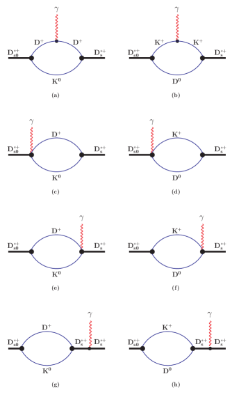
Figure 4: Diagrams contributing to the radiative transition $D_{s0}^{\ast+}\to D_{s}^{\ast+}+\gamma$.

Table 1. Coupling constant $g_{{}_{D_{s0}^{\ast}DK}}$.

The range of values for our results is due

to the variation of $\Lambda_{D_{s0}^{\ast}}$ from 1 to 2 GeV.

Approach	$g_{{}_{D_{s0}^{\ast}DK}}$ (GeV)
Ref. Nielsen:2006mi	2.5 - 3.8
Ref. Becirevic:1999fr	5.068
Ref. Colangelo:1995ph	5.5 $\pm$ 1.8
Ref. Wang:2006id	5.9${}^{+1.7}_{-1.6}$
Ref. Mehen:2004uj	6.0 - 7.8
Ref. Wang:2006bs	9.3${}^{+2.7}_{-2.1}$
Ref. Chow:1995ca	$<$ 9.86
Ref. Guo:2006fu	10.203
Our results:
NC case	9.90 $-$ 11.26
LC case	8.98
NCHQL case	11.52 $-$ 16.22
LCHQL case	11.52

Table 2. Decay width of $D_{s0}^{\ast}\to D_{s}\pi^{0}$.

The range of values for our results is due

to the variation of $\Lambda_{D_{s0}^{\ast}}$ from 1 to 2 GeV.

Approach	$\Gamma(D_{s0}^{\ast}\to D_{s}\pi^{0})$ (KeV)
Ref. Nielsen:2005zr	6 $\pm$ 2
Ref. Colangelo:2003vg	7 $\pm$ 1
Ref. Godfrey:2003kg	10
Ref. Fayyazuddin:2003dp	16
Ref. Bardeen:2003kt	21.5
Ref. Lu:2006ry	32
Ref. Wei:2005ag	39 $\pm$ 5
Ref. Ishida:2003gu	15 $-$ 70
Ref. Cheng:2003kg	10 $-$ 100
Ref. Azimov:2004xk	129 $\pm$ 43 (109 $\pm$ 16)
Our results:
Full case	46.7 $-$ 111.9
LO case	46.6 $-$ 112.6

Table 3. Decay width of $D_{s0}^{\ast}\to D_{s}^{\ast}\gamma\$.

The range of values for our results is due

to the variation of $\Lambda_{D_{s0}^{\ast}}$ from 1 to 2 GeV.

Approach	$\Gamma(D_{s0}^{\ast}\to D_{s}^{\ast}\gamma)\ \$ (KeV)
Ref. Fayyazuddin:2003dp	0.2
Ref. Colangelo:2003vg	0.85 $\pm$ 0.05
Ref. Close:2005se	1
Ref. Liu:2006jx	1.1
Ref. Wang:2006mf	1.3 $-$ 9.9
Ref. Azimov:2004xk	$\leq$ 1.4
Ref. Bardeen:2003kt	1.74
Ref. Godfrey:2003kg	1.9
Ref. Colangelo:2005hv	4 $-$ 6
Ref. Ishida:2003gu	21
Our results:
NC case	0.47 $-$ 0.63
LC case	0.66
NCHQL case	0.71 $-$ 1.17
LCHQL case	1.41

References

- (1) M. B. Voloshin and L. B. Okun, JETP Lett. 23, 333 (1976) [Pisma Zh. Eksp. Teor. Fiz. 23, 369 (1976)].
- (2) A. De Rujula, H. Georgi and S. L. Glashow, Phys. Rev. Lett. 38, 317 (1977).
- (3) S. F. Tuan, Phys. Rev. D 15, 3478 (1977); Phys. Lett. B 473, 136 (2000) [arXiv:hep-ph/9903342].
- (4) F. Gutbrod, G. Kramer and C. Rumpf, Z. Phys. C 1, 391 (1979).
- (5) J. D. Weinstein and N. Isgur, Phys. Rev. Lett. 48, 659 (1982); Phys. Rev. D 27, 588 (1983); Phys. Rev. D 41, 2236 (1990).
- (6) T. Barnes, Phys. Lett. B 165, 434 (1985).
- (7) T. Barnes, F. E. Close and H. J. Lipkin, Phys. Rev. D 68, 054006 (2003) [arXiv:hep-ph/0305025].
- (8) J. L. Rosner, Phys. Rev. D 74, 076006 (2006) [arXiv:hep-ph/0608102].
- (9) V. Baru, J. Haidenbauer, C. Hanhart, Yu. Kalashnikova and A. E. Kudryavtsev, Phys. Lett. B 586 (2004) 53 [arXiv:hep-ph/0308129]; C. Hanhart, Yu. S. Kalashnikova, A. E. Kudryavtsev and A. V. Nefediev, Phys. Rev. D 75, 074015 (2007) [arXiv:hep-ph/0701214].
- (10) E. van Beveren and G. Rupp, Phys. Rev. Lett. 91, 012003 (2003) [arXiv:hep-ph/0305035].
- (11) F. K. Guo, P. N. Shen, H. C. Chiang and R. G. Ping, Phys. Lett. B 641, 278 (2006) [arXiv:hep-ph/0603072].
- (12) F. K. Guo, P. N. Shen and H. C. Chiang, Phys. Lett. B 647, 133 (2007) [arXiv:hep-ph/0610008].
- (13) T. Barnes, S. Godfrey and E. S. Swanson, Phys. Rev. D 72, 054026 (2005) [arXiv:hep-ph/0505002].
- (14) B. Aubert et al. [BABAR Collaboration], Phys. Rev. Lett. 98, 012001 (2007) [arXiv:hep-ex/0603052].
- (15) X. G. He, X. Q. Li, X. Liu and X. Q. Zeng, arXiv:hep-ph/0606015.
- (16) B. Aubert et al. [BABAR Collaboration], Phys. Rev. Lett. 90, 242001 (2003) [arXiv:hep-ex/0304021].
- (17) D. Besson et al. [CLEO Collaboration], Phys. Rev. D 68, 032002 (2003) [arXiv:hep-ex/0305100].
- (18) Y. Mikami et al., Phys. Rev. Lett. 92 (2004) 012002 [arXiv:hep-ex/0307052].
- (19) P. Krokovny et al. [Belle Collaboration], Phys. Rev. Lett. 91, 262002 (2003) [arXiv:hep-ex/0308019].
- (20) B. Aubert et al. [BABAR Collaboration], Phys. Rev. Lett. 93, 181801 (2004) [arXiv:hep-ex/0408041].
- (21) W. M. Yao et al. [Particle Data Group], J. Phys. G 33, 1 (2006).
- (22) S. Godfrey, Phys. Lett. B 568, 254 (2003) [arXiv:hep-ph/0305122].
- (23) S. Godfrey and N. Isgur, Phys. Rev. D 32, 189 (1985); S. Godfrey and R. Kokoski, Phys. Rev. D 43, 1679 (1991).
- (24) M. A. Nowak, M. Rho and I. Zahed, Phys. Rev. D 48, 4370 (1993) [arXiv:hep-ph/9209272].
- (25) W. A. Bardeen and C. T. Hill, Phys. Rev. D 49, 409 (1994) [arXiv:hep-ph/9304265].
- (26) H. Y. Cheng and W. S. Hou, Phys. Lett. B 566, 193 (2003) [arXiv:hep-ph/0305038].
- (27) P. Colangelo and F. De Fazio, Phys. Lett. B 570, 180 (2003) [arXiv:hep-ph/0305140].
- (28) W. A. Bardeen, E. J. Eichten and C. T. Hill, Phys. Rev. D 68, 054024 (2003) [arXiv:hep-ph/0305049].
- (29) T. E. Browder, S. Pakvasa and A. A. Petrov, Phys. Lett. B 578, 365 (2004) [arXiv:hep-ph/0307054].
- (30) E. E. Kolomeitsev and M. F. M. Lutz, Phys. Lett. B 582, 39 (2004) [arXiv:hep-ph/0307133].
- (31) Fayyazuddin and Riazuddin, Phys. Rev. D 69, 114008 (2004) [arXiv:hep-ph/0309283].
- (32) S. Ishida, M. Ishida, T. Komada, T. Maeda, M. Oda, K. Yamada and I. Yamauchi, AIP Conf. Proc. 717, 716 (2004) [arXiv:hep-ph/0310061].
- (33) Y. I. Azimov and K. Goeke, Eur. Phys. J. A 21, 501 (2004) [arXiv:hep-ph/0403082].
- (34) M. Q. Huang, Phys. Rev. D 69, 114015 (2004) [arXiv:hep-ph/0404032].
- (35) D. S. Hwang and D. W. Kim, Phys. Lett. B 606, 116 (2005) [arXiv:hep-ph/0410301].
- (36) I. W. Lee, T. Lee, D. P. Min and B. Y. Park, Eur. Phys. J. C 49, 737 (2007) [arXiv:hep-ph/0412210].
- (37) Yu. A. Simonov and J. A. Tjon, Phys. Rev. D 70, 114013 (2004) [arXiv:hep-ph/0409361].
- (38) T. Mehen and R. P. Springer, Phys. Rev. D 70, 074014 (2004) [arXiv:hep-ph/0407181]; Phys. Rev. D 72, 034006 (2005) [arXiv:hep-ph/0503134].
- (39) P. Colangelo, F. De Fazio and A. Ozpineci, Phys. Rev. D 72, 074004 (2005) [arXiv:hep-ph/0505195].
- (40) F. E. Close and E. S. Swanson, Phys. Rev. D 72, 094004 (2005) [arXiv:hep-ph/0505206].
- (41) H. Kim and Y. Oh, Phys. Rev. D 72, 074012 (2005) [arXiv:hep-ph/0508251].
- (42) W. Wei, P. Z. Huang and S. L. Zhu, Phys. Rev. D 73, 034004 (2006) [arXiv:hep-ph/0510039].
- (43) M. Nielsen, Phys. Lett. B 634, 35 (2006) [arXiv:hep-ph/0510277].
- (44) X. Liu, Y. M. Yu, S. M. Zhao and X. Q. Li, Eur. Phys. J. C 47, 445 (2006) [arXiv:hep-ph/0601017].
- (45) J. Lu, X. L. Chen, W. Z. Deng and S. L. Zhu, Phys. Rev. D 73, 054012 (2006) [arXiv:hep-ph/0602167].
- (46) T. M. Aliev and M. Savci, Phys. Rev. D 73, 114010 (2006) [arXiv:hep-ph/0604002].
- (47) T. M. Aliev, K. Azizi and A. Ozpineci, arXiv:hep-ph/0608264.
- (48) H. Y. Cheng and C. K. Chua, Phys. Rev. D 74, 034020 (2006) [arXiv:hep-ph/0605073].
- (49) Z. G. Wang and S. L. Wan, Phys. Rev. D 73, 094020 (2006) [arXiv:hep-ph/0603007].
- (50) Z. G. Wang, Phys. Rev. D 75, 034013 (2007) [arXiv:hep-ph/0612225]; J. Phys. G 34, 753 (2007) [arXiv:hep-ph/0611271].
- (51) M. Nielsen, arXiv:hep-ph/0610320.
- (52) D. Gamermann, E. Oset, D. Strottman and M. J. V. Vacas, arXiv:hep-ph/0612179.
- (53) S. M. Zhao, X. Liu and S. J. Li, arXiv:hep-ph/0612008.
- (54) S. Weinberg, Phys. Rev. 130, 776 (1963); A. Salam, Nuovo Cim. 25, 224 (1962); K. Hayashi, M. Hirayama, T. Muta, N. Seto and T. Shirafuji, Fortsch. Phys. 15, 625 (1967).
- (55) G. V. Efimov and M. A. Ivanov, The Quark Confinement Model of Hadrons, (IOP Publishing, Bristol Philadelphia, 1993).
- (56) D. Lurie and A. J. Macfarlane, Phys. Rev. 136 (1964) B816; D. Lurie and G. B. Tupper, Phys. Rev. D 47 (1993) 3580; M. D. Scadron, Phys. Rev. D 57, 5307 (1998) [arXiv:hep-ph/9712425].
- (57) G. V. Efimov, M. A. Ivanov and V. E. Lyubovitskij, Sov. J. Nucl. Phys. 48, 126 (1988) [Yad. Fiz. 48, 198 (1988)]; Few Body Syst. 6, 17 (1989) [Acta Phys. Austriaca 6, 17 (1989)]; I. V. Anikin, M. A. Ivanov, N. B. Kulimanova and V. E. Lyubovitskij, Z. Phys. C 65, 681 (1995); Phys. Atom. Nucl. 57, 1021 (1994) [Yad. Fiz. 57, 1082 (1994)]; M. A. Ivanov, M. P. Locher and V. E. Lyubovitskij, Few Body Syst. 21, 131 (1996). M. A. Ivanov, V. E. Lyubovitskij, J. G. Körner and P. Kroll, Phys. Rev. D 56, 348 (1997) [arXiv:hep-ph/9612463]; M. A. Ivanov, J. G. Körner and V. E. Lyubovitskij, Phys. Lett. B 448, 143 (1999) [arXiv:hep-ph/9811370]; M. A. Ivanov, J. G. Körner, V. E. Lyubovitskij, M. A. Pisarev and A. G. Rusetsky, Phys. Rev. D 61, 114010 (2000) [arXiv:hep-ph/9911425]; M. A. Ivanov, J. G. Körner, V. E. Lyubovitskij and A. G. Rusetsky, Phys. Rev. D 60, 094002 (1999) [arXiv:hep-ph/9904421]; Phys. Lett. B 476, 58 (2000) [arXiv:hep-ph/9910342]; M. A. Ivanov and P. Santorelli, Phys. Lett. B 456, 248 (1999) [arXiv:hep-ph/9903446]; A. Faessler, T. Gutsche, M. A. Ivanov, J. G. Körner and V. E. Lyubovitskij, Phys. Lett. B 518, 55 (2001) [arXiv:hep-ph/0107205]; M. A. Ivanov, J. G. Korner and P. Santorelli, Phys. Rev. D 73, 054024 (2006) [arXiv:hep-ph/0602050]; A. Faessler, T. Gutsche, M. A. Ivanov, J. G. Korner, V. E. Lyubovitskij, D. Nicmorus and K. Pumsa-ard, Phys. Rev. D 73, 094013 (2006) [arXiv:hep-ph/0602193]; A. Faessler, T. Gutsche, B. R. Holstein, V. E. Lyubovitskij, D. Nicmorus and K. Pumsa-ard, Phys. Rev. D 74, 074010 (2006) [arXiv:hep-ph/0608015].
- (58) A. Faessler, T. Gutsche, M. A. Ivanov, V. E. Lyubovitskij and P. Wang, Phys. Rev. D 68, 014011 (2003) [arXiv:hep-ph/0304031].
- (59) G. V. Efimov and S. N. Nedelko, Phys. Rev. D 51, 176 (1995); Y. V. Burdanov, G. V. Efimov, S. N. Nedelko and S. A. Solunin, Phys. Rev. D 54, 4483 (1996) [arXiv:hep-ph/9601344].
- (60) I. V. Anikin, A. E. Dorokhov and L. Tomio, Phys. Part. Nucl. 31, 509 (2000) [Fiz. Elem. Chast. Atom. Yadra 31, 1023 (2000)].
- (61) J. V. Burdanov and G. V. Efimov, Phys. Rev. D 64, 014001 (2001) [arXiv:hep-ph/0009027].
- (62) P. L. Cho and M. B. Wise, Phys. Rev. D 49, 6228 (1994) [arXiv:hep-ph/9401301].
- (63) D. J. Gross, S. B. Treiman and F. Wilczek, Phys. Rev. D 19, 2188 (1979); J. Gasser and H. Leutwyler, Phys. Rept. 87, 77 (1982).
- (64) V. M. Belyaev, V. M. Braun, A. Khodjamirian and R. Ruckl, Phys. Rev. D 51, 6177 (1995) [arXiv:hep-ph/9410280].
- (65) A. Anastassov et al. [CLEO Collaboration], Phys. Rev. D 65, 032003 (2002) [arXiv:hep-ex/0108043].
- (66) M. B. Wise, Phys. Rev. D 45, R2188 (1992); G. Burdman and J. F. Donoghue, Phys. Lett. B 280, 287 (1992).
- (67) Z. G. Wang and S. L. Wan, Phys. Rev. D 74, 014017 (2006) [arXiv:hep-ph/0606002].
- (68) M. E. Bracco, A. J. Cerqueira, M. Chiapparini, A. Lozea and M. Nielsen, Phys. Lett. B 641, 286 (2006) [arXiv:hep-ph/0604167].
- (69) K. L. Haglin, Phys. Rev. C 61, 031902 (2000) [arXiv:nucl-th/9907034].
- (70) R. S. Azevedo and M. Nielsen, Phys. Rev. C 69, 035201 (2004) [arXiv:nucl-th/0310061].
- (71) S. Mandelstam, Annals Phys. 19, 1 (1962); J. Terning, Phys. Rev. D 44, 887 (1991).
- (72) D. Becirevic and A. L. Yaouanc, JHEP 9903, 021 (1999) [arXiv:hep-ph/9901431].
- (73) P. Colangelo, F. De Fazio, G. Nardulli, N. Di Bartolomeo and R. Gatto, Phys. Rev. D 52, 6422 (1995) [arXiv:hep-ph/9506207].
- (74) C. K. Chow and D. Pirjol, Phys. Rev. D 54, 2063 (1996) [arXiv:hep-ph/9512242].