Power Allocation for Discrete-Input Non-Ergodic Block-Fading Channels

Abstract

We consider power allocation algorithms for fixed-rate transmission over Nakagami-$m$ non-ergodic block-fading channels with perfect transmitter and receiver channel state information and discrete input signal constellations under short- and long-term power constraints. Optimal power allocation schemes are shown to be direct applications of previous results in the literature. We show that the SNR exponent of the optimal short-term scheme is given by the Singleton bound. We also illustrate the significant gains available by employing long-term power constraints. Due to the nature of the expressions involved, the complexity of optimal schemes may be prohibitive for system implementation. We propose simple sub-optimal power allocation schemes whose outage probability performance is very close to the minimum outage probability obtained by optimal schemes.

I Introduction

The non-ergodic block-fading channel introduced in [1] and [2] models communication scenarios where each codeword spans a fixed number of independently faded blocks. The block-fading channel is an accurate model for slowly-varying fading scenarios encountered with slow time-frequency hopping or orthogonal frequency division multiplexing (OFDM).

Since each codeword experiences a finite number of degrees of freedom, the channel is non-ergodic. Therefore, the channel has zero capacity under most common fading statistics. A useful measure for the channel reliability in non-ergodic channels is the outage probability, which is the probability that a given communication rate is not supported by the channel [1, 2]. The outage probability is the lowest possible word error probability for sufficiently long codes.

When knowledge of channel parameters, referred to as channel state information (CSI), is not available at the transmitter, transmit power is allocated uniformly over the blocks. When CSI is available at the transmitter, power allocation techniques can be used to increase the instantaneous mutual information, thus improving the outage performance. Optimal power allocation schemes, minimizing the outage probability, have been studied under various power constraints. For systems with short-term power constraints (per-codeword power constraint), water-filling is the optimal power allocation scheme [3]. In [4] the power allocation problem is solved under long-term power constraint, showing that remarkable gains are possible with respect to short-term power allocation. For channels with two or more fading blocks, zero outage can be obtained under long-term power constraint. In both cases, the optimal input distribution is Gaussian.

In [5], the authors propose the optimal short-term power allocation scheme to maximize the mutual information of parallel channels for arbitrary input distributions. Also, as mentioned in [5], optimal short-term power allocation for block-fading channels with discrete inputs is obtained directly from their results. Due to its complexity, the optimal solution in [5] does not provide much insight into the impact of the parameters involved, and may also prohibit the application to systems with strict memory and computational constraints.

In this paper, we study optimal short- and long-term power allocation schemes for fixed-rate transmission over discrete-input block-fading channels with perfect CSI at the transmitter and receiver. We consider non-causal CSI, namely, the channel gains corresponding to the transmission of one codeword are known to the transmitter and receiver. In practice, this non-causal assumption reflects the situation of OFDM, where the time-domain channel is estimated but the signals are transmitted in the frequency domain. In particular, we show that the SNR exponent for optimal short-term allocation is given by the Singleton bound [6, 7, 8]. Furthermore, we show that the results in [5] are instrumental in obtaining the optimal long-term solution. We further aim at reducing the complexity drawbacks of optimal schemes by proposing suboptimal short- and long-term power allocation schemes. The suboptimal schemes are simpler as compared to the corresponding optimal schemes, yet they suffer only negligible losses compared to the optimal performance. Proofs of all results can be found in [9].

II System Model

Consider transmission over an additive white Gaussian noise (AWGN) block-fading channel with $B$ blocks of $L$ channel uses each, in which, for $b=1,\ldots,B$, block $b$ is affected by a flat fading coefficient $h_{b}\in\mathbb{C}$. Let $\gamma_{b}=|h_{b}|^{2}$ be the power fading gain and assume that the fading gain vector $\mbox{\boldmath{$\gamma$}}=(\gamma_{1},\ldots,\gamma_{B})$ is available at both the transmitter and the receiver. The transmit power is allocated to the blocks according to the scheme $\mathbf{p}(\mbox{\boldmath{$\gamma$}})=(p_{1}(\mbox{\boldmath{$\gamma$}}),\ldots,p_{B}(\mbox{\boldmath{$\gamma$}}))$. Then, the complex baseband channel model can be written as

$$\mathbf{y}_{b}=\sqrt{p_{b}(\mbox{\boldmath{$\gamma$}})}h_{b}\mathbf{x}_{b}+\mathbf{z}_{b},\ \ b=1,\ldots,B,$$ (1)

where $\mathbf{y}_{b}\in\mathbb{C}^{L}$ is the received signal in block $b$, $\mathbf{x}_{b}\in\mathcal{X}^{L}\subset\mathbb{C}^{L}$ is the portion of the codeword being transmitted in block $b$, $\mathcal{X}\subset\mathbb{C}$ is the signal constellation and $\mathbf{z}_{b}\in\mathbb{C}^{L}$ is a noise vector with independent, identically distributed (i.i.d.) circularly symmetric Gaussian entries $\sim\mathcal{N}_{\mathbb{C}}(0,1)$. Assume that the signal constellation $\mathcal{X}$ is normalized in energy such that $\sum_{x\in\mathcal{X}}|x|^{2}=2^{M}$, where $M=\log_{2}|\mathcal{X}|$. Then, the instantaneous received SNR at block $b$ is given by $p_{b}(\mbox{\boldmath{$\gamma$}})\gamma_{b}$.

We consider block-fading channels where $h_{b}$ are realizations of a random variable $H$, whose magnitude is Nakagami-$m$-distributed and has a uniformly distributed phase. The fading magnitude has the following probability density function (pdf)

$$f_{|H|}(h)=\frac{2m^{m}h^{2m-1}}{\Gamma(m)}e^{-mh^{2}},$$ (2)

where $\Gamma(a)$ is the Gamma function, $\Gamma(a)=\int_{0}^{\infty}t^{a-1}e^{-t}dt$. The coefficients $\gamma_{b}$ are realizations of the random variable $|H|^{2}$ whose pdf is given by

$$f_{|H|^{2}}(\gamma)=\begin{cases}\frac{m^{m}\gamma^{m-1}}{\Gamma(m)}e^{-m\gamma},&\gamma\geq 0\\ 0,&{\rm otherwise}.\end{cases}$$ (3)

The Nakagami-$m$ distribution encompasses many fading distributions of interest. In particular, we obtain Rayleigh fading by letting $m=1$ and Rician fading with parameter $K$ by setting $m=(K+1)^{2}/(2K+1)$.

III Mutual Information and Outage Probability

For any given power fading gain realization $\gamma$ and power allocation scheme $\mathbf{p}(\mbox{\boldmath{$\gamma$}})$, the instantaneous input-output mutual information of the channel is given by

$$I_{B}(\mathbf{p}(\mbox{\boldmath{$\gamma$}}),\mbox{\boldmath{$\gamma$}})=\frac{1}{B}\sum_{b=1}^{B}I_{\mathcal{X}}(p_{b}\gamma_{b}),$$ (4)

where $I_{\mathcal{X}}(\rho)$ is the input-output mutual information of an AWGN channel with input constellation ${\mathcal{X}}$ received SNR $\rho$

$$I_{\mathcal{X}}(\rho)=M-\mathbb{E}_{X,Z}\left[\log_{2}\left(\sum_{x^{\prime}\in\mathcal{X}}e^{-|\sqrt{\rho}(X-x^{\prime})+Z|^{2}+|Z|^{2}}\right)\right].$$

Communication is in outage when the instantaneous input-output mutual information is less than the target rate $R$. For a given power allocation scheme $\mathbf{p}(\mbox{\boldmath{$\gamma$}})$, the outage probability at communication rate $R$ is given by [1, 2]

$$P_{\rm out}(\mathbf{p}(\mbox{\boldmath{$\gamma$}}),R) =\Pr(I_{B}(\mathbf{p}(\mbox{\boldmath{$\gamma$}}),\mbox{\boldmath{$\gamma$}})<R)$$

$$=\Pr\left(\frac{1}{B}\sum_{b=1}^{B}I_{\mathcal{X}}(p_{b}\gamma_{b})<R\right).$$ (5)

IV Short-Term Power Allocation

Short-term power allocation schemes are applied for systems where the transmit power of each codeword is limited to $BP$. A given short-term power allocation scheme $\mathbf{p(\mbox{\boldmath{$\gamma$}})}=(p_{1},\ldots,p_{B})$ must then satisfy $\sum_{b=1}^{B}p_{b}\leq BP$.

IV-A Optimal Power Allocation

The optimal short-term power allocation rule $\mathbf{p}^{\rm opt}(\mbox{\boldmath{$\gamma$}})$ is the solution to the outage probability minimization problem [4]. Mathematically we express $\mathbf{p}^{\rm opt}(\mbox{\boldmath{$\gamma$}})$ as

$$\mathbf{p}^{\rm opt}(\mbox{\boldmath{$\gamma$}})=\arg\min_{\begin{subarray}{c}{\mathbf{p}}\in\mathbb{R}^{B}_{+}\\ \sum_{b=1}^{B}p_{b}=BP\end{subarray}}P_{\rm out}(\mathbf{p(\mbox{\boldmath{$\gamma$}})},R).$$ (6)

For short-term power allocation, since the available power can only be distributed within one codeword, the power allocation scheme that maximizes the instantaneous mutual information at each channel realization also minimizes the outage probability. Formally, we have [4]

Lemma 1

Let $\mathbf{p}^{\rm opt}(\mbox{\boldmath{$\gamma$}})$ be a solution of the problem

$$\left\{\begin{array}[]{ll}{\rm Maximize}&\sum_{b=1}^{B}I_{\mathcal{X}}(p_{b}\gamma_{b})\\ {\rm Subject\ to}&\sum_{b=1}^{B}p_{b}\leq BP\\ &p_{b}\geq 0,b=1,\ldots,B.\end{array}\right.$$ (7)

Then $\mathbf{p}^{\rm opt}(\mbox{\boldmath{$\gamma$}})$ is a solution of $\eqref{eq:opt_short_prob}$.

From [5], the solution for problem (7) is given by

$$p^{\rm opt}_{b}(\mbox{\boldmath{$\gamma$}})=\frac{1}{\gamma_{b}}{\rm MMSE}_{\mathcal{X}}^{-1}\left(\min\left\{1,\frac{\nu}{\gamma_{b}}\right\}\right),$$ (8)

for $b=1,\dotsc,B$, where ${\rm MMSE}_{\mathcal{X}}(\rho)$ is the minimum mean-squared error (MMSE) for estimating the input based on the received signal over an AWGN channel with SNR $\rho$

$${\rm MMSE}_{\mathcal{X}}(\rho)=1-\frac{1}{\pi}\int_{\mathbb{C}}\frac{\left|\sum_{x\in\mathcal{X}}xe^{-|y-\sqrt{\rho}x|^{2}}\right|^{2}}{\sum_{x\in\mathcal{X}}e^{-|y-\sqrt{\rho}x|^{2}}}dy$$ (9)

and $\nu$ is chosen such that the power constraint is satisfied,

$$\sum_{b=1}^{B}p^{\rm opt}_{b}=BP.$$ (10)

The optimal short-term power allocation scheme improves the outage performance of block-fading systems. However, it does not increase the outage diversity compared to uniform power allocation, as shown in the following lemma.

Lemma 2

Consider transmission over the block-fading channel defined in (1) with the optimal power allocation scheme $\mathbf{p}^{\rm opt}(\mbox{\boldmath{$\gamma$}})$ given in (8). Assume input constellation size $|\mathcal{X}|=2^{M}$. Further assume that the power fading gains follow the distribution given in (3). Then, for large $P$ and some $\mathcal{K}_{\rm opt}>0$ the outage probability behaves as

$$P_{\rm out}(\mathbf{p^{\rm opt}}(\mbox{\boldmath{$\gamma$}}),R)\doteq\mathcal{K}_{\rm opt}P^{-md_{B}(R)},$$ (11)

where $d_{B}(R)$ is the Singleton bound given by

$$d_{B}(R)=1+\left\lfloor B\left(1-\frac{R}{M}\right)\right\rfloor$$ (12)

IV-B Suboptimal Power Allocation Schemes

Although the power allocation scheme in (8) is optimal, it involves an inverse MMSE function, which may be too complex to implement or store for specific low-cost systems. Moreover, the MMSE function provides little insight to the role of each parameter. In this section, we propose power allocation schemes similar to water-filling that tackle both drawbacks and perform very close to the optimal solution.

IV-B1 Truncated water-filling scheme

The complexity of the solution in (8) is due to the complex expression of $I_{\mathcal{X}}(\rho)$ in problem (7). Therefore, in order to obtain a simple suboptimal solution, we find an aproximation for $I_{\mathcal{X}}(\rho)$ in problem (7). The water-filling solution in [4] suggests the following approximation of $I_{\mathcal{X}}(\rho)$

$$I^{\rm tw}(\rho)=\left\{\begin{array}[]{ll}\log_{2}(1+\rho),&\rho\leq\beta\\ \log_{2}(1+\beta),&\rm{otherwise,}\end{array}\right.$$ (13)

where $\beta$ is a design parameter to be optimized for best performance. The resulting suboptimal scheme $\mathbf{p^{\rm tw}}(\mbox{\boldmath{$\gamma$}})$ is given as a solution of

$$\left\{\begin{array}[]{ll}\rm{Maximize}&\sum_{b=1}^{B}I^{\rm tw}(p_{b}\gamma_{b})\\ \rm{Subject\ to}&\sum_{b=1}^{B}p_{b}\leq BP\\ &p_{b}\geq 0,\ b=1,\ldots,B.\end{array}\right.$$ (14)

Lemma 3

A solution to the problem (14) is given by

$$p^{\rm tw}_{b}(\mbox{\boldmath{$\gamma$}})=\begin{cases}\frac{\beta}{\gamma_{b}},&{\rm if}\sum_{b=1}^{B}\frac{\beta}{\gamma_{b}}\leq BP\\ \min\left\{\frac{\beta}{\gamma_{b}},\left(\eta-\frac{1}{\gamma_{b}}\right)_{+}\right\},&{\rm otherwise}\end{cases}$$ (15)

for $b=1,\ldots,B$, where $\eta$ is chosen such that

$$\sum_{b=1}^{B}\min\left\{\frac{\beta}{\gamma_{b}},\left(\eta-\frac{1}{\gamma_{b}}\right)_{+}\right\}=BP.$$ (16)

Without loss of generality, assume that $\gamma_{1}\geq\ldots\geq\gamma_{B}$, then, similarly to water-filling, $\eta$ can be determined such that [4]

$$(k-l)\eta=BP-\sum_{b=1}^{l}\frac{\beta+1}{\gamma_{b}}+\sum_{b=1}^{k}\frac{1}{\gamma_{b}}$$ (17)

where $k,l$ are integers satisfying $\frac{1}{\gamma_{k}}<\eta<\frac{1}{\gamma_{k+1}}$ and $\frac{\beta+1}{\gamma_{l}}<\eta\leq\frac{\beta+1}{\gamma_{l+1}}$.

From Lemma 3, the resulting power allocation scheme is similar to water-filling, except for the truncation of the allocated power at $\frac{\beta}{\gamma_{b}}$. We refer to this scheme as truncated water-filling.

The outage performance obtained by the truncated water-filling scheme depends on the choice of the design parameter $\beta$. We now analyze the asymptotic performance of the outage probability, thus providing some guidance on the choice of $\beta$.

Lemma 4

Consider transmission over the block-fading channel defined in (1) with the truncated water-filling power allocation scheme $\mathbf{p}^{\rm tw}(\mbox{\boldmath{$\gamma$}})$ given in (15). Assume input constellation $\mathcal{X}$ of size $|\mathcal{X}|=2^{M}$. Further assume that the power fading gains follow the distribution given in (3). Then, for large $P$, the outage probability $P_{\rm out}(\mathbf{p^{\rm tw}}(\mbox{\boldmath{$\gamma$}}),R)$ is asymptotically upper bounded by

$$P_{\rm out}(\mathbf{p^{\rm tw}}(\mbox{\boldmath{$\gamma$}}),R)\dot{\leq}\mathcal{K}_{\beta}P^{-md_{\beta}(R)},$$ (18)

where

$$d_{\beta}(R)=1+\left\lfloor B\left(1-\frac{R}{I_{\mathcal{X}}(\beta)}\right)\right\rfloor,$$ (19)

and $I_{\mathcal{X}}(\beta)$ is the input-output mutual information of an AWGN channel with SNR $\beta$.

From the results of Lemmas 2 and 4, we note that $P_{\rm out}(\mathbf{p^{\rm tw}}(\mbox{\boldmath{$\gamma$}}),R)\geq P_{\rm out}(\mathbf{p^{\rm opt}(\mbox{\boldmath{$\gamma$}})},R)$, and we have that

$$P_{\rm out}(\mathbf{p^{\rm tw}}(\mbox{\boldmath{$\gamma$}}),R)\doteq\mathcal{K}_{\rm tw}P^{-md_{\rm tw}(R)},$$ (20)

where $d_{\rm tw}(R)$ satisfies that $d_{\beta}(R)\leq d_{\rm tw}(R)\leq d_{B}(R)$.

Therefore, the truncated water-filling scheme is guaranteed to obtain optimal diversity whenever $d_{\beta}(R)=d_{B}(R)$, or equivalently, when

$$B\left(1-\frac{R}{I_{\mathcal{X}}(\beta)}\right) \geq\left\lfloor B\left(1-\frac{R}{M}\right)\right\rfloor$$ (21)

$$I_{\mathcal{X}}(\beta) \geq\frac{BR}{B-\left\lfloor B\left(1-\frac{R}{M}\right)\right\rfloor}$$ (22)

which implies that

$$\beta\geq I_{\mathcal{X}}^{-1}\left(\frac{BR}{B-\left\lfloor B\left(1-\frac{R}{M}\right)\right\rfloor}\right)\triangleq\beta_{R}.$$

Therefore, the truncated water-filling power allocation scheme (15) becomes the classical water-filling algorithm for Gaussian inputs, and provides optimal outage diversity at any transmission rate by letting $\beta\rightarrow\infty$. For any rate $R$ that is not at the discontinuity points of the Singleton bound, i.e. $R$ such that $B\left(1-\frac{R}{M}\right)$ is not an integer, we can always design a truncated water-filling scheme that obtains optimal diversity by choosing $\beta\geq\beta_{R}$.

With the results above, we choose $\beta$ as follows. For a transmission rate $R$ that is not a discontinuity point of the Singleton bound, we perform a simulation to compute the outage probability at rate $R$ obtained by truncated water-filling with various $\beta\geq\beta_{R}$ and pick the $\beta$ that gives the best outage performance. The dashed line in Figure 1 illustrates the performance of the obtained schemes for block-fading channels with $B=4$, QPSK input under Rayleigh fading. At all rates of interest, the truncated water-filling schemes perform very close to the optimal scheme (solid line), especially at high SNR.

Figure 1: Outage performance of various short-term power allocation schemes for QPSK-input block-fading channels with $B=4$ and Rayleigh fading. The solid-line represents optimal scheme; the solid line with $\diamond$ represents uniform power allocation; the dashed line and dashed-dotted line represent truncated water-filling and its corresponding refinement, respectively; the dotted line represents classical water-filling scheme.

For rates at the discontinuous points of the Singleton bound, especially when operating at high SNR, $\beta$ needs to be relatively large in order to maintain diversity. However, large $\beta$ increases the gap between $I^{\rm tw}(\rho)$ and $I_{\mathcal{X}}(\rho)$, thus degrades the performance of the truncated water-filling scheme. For $\beta=15$, the gap is illustrated by the dashed lines in Figure 2. In the extreme case where $\beta\to\infty$, the truncated water-filling turns into the water-filling scheme, which exhibits a significant loss in outage performance as illustrated by the dotted lines in Figure 1. To reduce this drawback, we propose a better approximation to $I_{\mathcal{X}}(\rho)$, which leads to a refinement to the truncated water-filling scheme in the next section.

IV-B2 Refined truncated water-filling schemes

To obtain better approximation to the optimal power allocation scheme, we need a more accurate approximation to $I_{\mathcal{X}}(\rho)$ in (7). We propose the following approximation

$$I^{\rm ref}(\rho)=\left\{\begin{array}[]{ll}\log_{2}(1+\rho),&\rho\leq\alpha\\ \kappa\log_{2}(\rho)+a,&\alpha<\rho\leq\beta\\ \kappa\log_{2}(\beta)+a,&{\rm otherwise,}\end{array}\right.$$ (23)

where $\kappa$ and $a$ are chosen such that in dB scale, $\kappa\log_{2}(\rho)+a$ is a tangent to $I_{\mathcal{X}}(\rho)$ at a predetermined point $\rho_{0}$. Therefore $\alpha$ is chosen such that $\kappa\log_{2}(\alpha)+a=\log_{2}(1+\alpha)$, and $\beta$ is a design parameter. For QPSK input and $\rho_{0}=3$, we have $\kappa=0.3528,a=1.1327,\alpha=1.585$.

The optimization problem (7) is approximated by

$$\left\{\begin{array}[]{ll}{\rm Maximize}&\sum_{b=1}^{B}I^{\rm ref}(p_{b}\gamma_{b})\\ {\rm Subject\ to}&\sum_{b=1}^{B}p_{b}\leq BP\\ &p_{b}\geq 0,b=1,\ldots,B.\end{array}\right.$$ (24)

The refined truncated water-filling scheme $\mathbf{p^{\rm ref}}(\mbox{\boldmath{$\gamma$}})$ is given by the following lemma.

Lemma 5

A solution to problem (24) is

$$p^{\rm ref}_{b}=\frac{\beta}{\gamma_{b}},\,\,\,b=1,\ldots,B$$ (25)

if $\sum_{b=1}^{B}\frac{\beta}{\gamma_{b}}<BP$, and otherwise, for $b=1,\ldots,B$,

$$p^{\rm ref}_{b}=\begin{cases}\frac{\beta}{\gamma_{b}},&\eta\geq\frac{\beta}{\kappa\gamma_{b}}\\ \kappa\eta,&\frac{\alpha}{\kappa\gamma_{b}}\leq\eta<\frac{\beta}{\kappa\gamma_{b}}\\ \frac{\alpha}{\gamma_{b}},&\frac{\alpha+1}{\gamma_{b}}\leq\eta<\frac{\alpha}{\kappa\gamma_{b}}\\ \eta-\frac{1}{\gamma_{b}},&\frac{1}{\gamma_{b}}\leq\eta<\frac{\alpha+1}{\gamma_{b}}\\ 0,&{\rm otherwise,}\end{cases}$$ (26)

where $\eta$ is chosen such that

$$\sum_{b=1}^{B}p^{\rm ref}_{b}=BP.$$ (27)

The refined truncated water-filling scheme provides significant gain over the truncated water-filling scheme, especially when the transmission rate requires relatively large $\beta$ to maintain the outage diversity. The dashed-dotted lines in Figure 2 show the outage performance of the refined truncated water-filling scheme for block-fading channels with $B=4$, QPSK input under Rayleigh fading. The refined truncated water-filling scheme performs very close to the optimal case even at the rates where the Singleton bound is discontinuous, i.e. rates $R=0.5,1.0,1.5$. The performance gains of the refined scheme over the truncated water-filling scheme at other rates are also illustrated by the dashed-dotted lines in Figure 1.

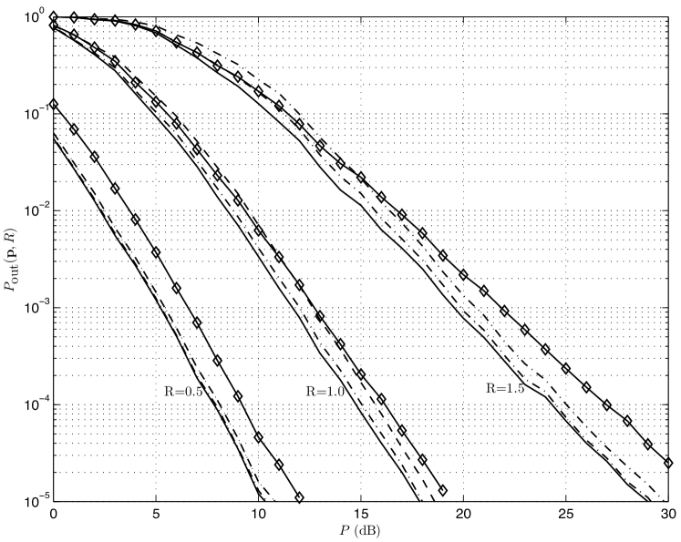
Figure 2: Outage performance of various short-term power allocation schemes for QPSK-input block-fading channels with $B=4$ and Rayleigh fading. The solid-line represents optimal scheme; the solid line with $\diamond$ represents uniform power allocation; the dashed line and dashed-dotted line correspondingly represent truncated water-filling and its refinement with $\beta=15$.

V Long-Term Power Allocation

We consider systems with long-term power constraints, in which the expectation of the power allocated to each block (over infinitely many codewords) does not exceed $P$. This problem has been investigated in [4] for block-fading channels with Gaussian inputs. In this section, we obtain similar results for channels with discrete inputs, and propose suboptimal schemes that reduce the complexity of the algorithm.

V-A Optimal Long-Term Power Allocation

Following [4], the problem can be formulated as

$$\left\{\begin{array}[]{ll}{\rm Minimize}&\Pr(I_{B}(\mathbf{p}_{\rm lt}(\mbox{\boldmath{$\gamma$}}),\mbox{\boldmath{$\gamma$}})<R)\\ {\rm Subject\ to}&\mathbb{E}\left[\langle\mathbf{p}_{\rm lt}(\mbox{\boldmath{$\gamma$}})\rangle\right]\leq P,\\ \end{array}\right.$$ (28)

where $\langle\mathbf{p}\rangle=\frac{1}{B}\sum_{b=1}^{B}p_{b}$.

The following theorem shows that the structure of the optimal long-term solution $\mathbf{p^{\rm opt}_{\rm lt}}(\mbox{\boldmath{$\gamma$}})$ of [4] for Gaussian inputs is generalized to the discrete-input case.

Theorem 1

Problem (28) is solved by $\mathbf{p^{\rm opt}_{\rm lt}}(\mbox{\boldmath{$\gamma$}})$ given by

$$\mathbf{p^{\rm opt}_{\rm lt}}(\mbox{\boldmath{$\gamma$}})=\left\{\begin{array}[]{ll}\mbox{\boldmath{$\wp$}}^{\rm opt}(\mbox{\boldmath{$\gamma$}}),&{\rm if\ }\mbox{\boldmath{$\gamma$}}\in\mathcal{R}(s^{\star})\\ 0,&{\rm if\ }\mbox{\boldmath{$\gamma$}}\notin\overline{\mathcal{R}}(s^{\star}),\end{array}\right.$$ (29)

while if $\mbox{\boldmath{$\gamma$}}\in\overline{\mathcal{R}}(s^{\star})\setminus\mathcal{R}(s^{\star})$ then $\mathbf{p^{\rm opt}_{\rm lt}}(\mbox{\boldmath{$\gamma$}})=\mbox{\boldmath{$\wp$}}(\mbox{\boldmath{$\gamma$}})$ with probability $w^{\star}$ and $\mathbf{p^{\rm opt}_{\rm lt}}(\mbox{\boldmath{$\gamma$}})=0$ with probability $1-w^{\star}$, where $\mbox{\boldmath{$\wp$}}(\mbox{\boldmath{$\gamma$}})$ is the solution of the following optimization problem

$$\left\{\begin{array}[]{ll}{\rm Minimize}&\langle\mbox{\boldmath{$\wp$}}\rangle\\ {\rm Subject\ to}&\sum_{b=1}^{B}I_{\mathcal{X}}(\wp_{b}\gamma_{b})\geq BR\\ &\wp_{b}\geq 0,b=1,\ldots,B,\end{array}\right.$$ (30)

and $\mathcal{R}(s),\overline{\mathcal{R}}(s),s^{\star},w^{\star}$ are defined as follows

$${\mathcal{R}}(s) =\{\mbox{\boldmath{$\gamma$}}\in\mathbb{R}_{+}^{B}:\langle\mbox{\boldmath{$\wp$}}^{\rm opt}(\mbox{\boldmath{$\gamma$}})\rangle<s\}$$ (31)

$$\overline{\mathcal{R}}(s) =\{\mbox{\boldmath{$\gamma$}}\in\mathbb{R}_{+}^{B}:\langle\mbox{\boldmath{$\wp$}}^{\rm opt}(\mbox{\boldmath{$\gamma$}})\rangle\leq s\}$$ (32)

$$s^{\star} =\sup\{s:P(s)<P\}$$ (33)

$$w^{\star} =\frac{P-P(s^{\star})}{\overline{P}(s^{\star})-P(s^{\star})}$$ (34)

where

$$P(s) =\mathbb{E}_{\mbox{\boldmath{$\gamma$}}\in\mathcal{R}(s)}\left[\langle\mbox{\boldmath{$\wp$}}^{\rm opt}(\mbox{\boldmath{$\gamma$}})\rangle\right]$$ (35)

$$\overline{P}(s) =\mathbb{E}_{\mbox{\boldmath{$\gamma$}}\in\overline{\mathcal{R}}(s)}\left[\langle\mbox{\boldmath{$\wp$}}^{\rm opt}(\mbox{\boldmath{$\gamma$}})\rangle\right]$$ (36)

and $\mbox{\boldmath{$\wp$}}^{\rm opt}(\mbox{\boldmath{$\gamma$}})$ is the solution of (30) given by

$$\wp^{\rm opt}_{b}=\left\{\begin{array}[]{ll}\frac{1}{\gamma_{b}}{\rm MMSE}_{\mathcal{X}}^{-1}\left(\frac{1}{\eta\gamma_{b}}\right),&\eta\geq\frac{1}{\gamma_{b}}\\ 0,&{\rm otherwise}\end{array}\right.$$ (37)

for $b=1,\ldots,B$, where $\eta$ is chosen such that

$$\sum_{b=1;\gamma_{b}\geq\frac{1}{\eta}}^{B}I_{\mathcal{X}}\left({\rm MMSE}_{\mathcal{X}}^{-1}\left(\frac{1}{\eta\gamma_{b}}\right)\right)=BR.$$ (38)

As in the Gaussian input case [4], the optimal power allocation scheme either transmits with the minimum power that enables transmission at the target rate, or turns off transmission (allocating zero power) when the channel realization is bad. Therefore, there is no power wastage on outage events.

The solid lines in Figure 3 illustrates the outage performance of optimal long-term power allocation schemes for transmission over 4-block block-fading channels with QPSK-input and Rayleigh fading. The simulation results suggest that for communication rates where $d_{B}(R)>1$, zero outage probability can be obtained with finite power. This agrees to the results obtained for block-fading channels with Gaussian inputs [4], where only for $B>1$ zero outage was possible.

V-B Suboptimal Long-Term Power Allocation

In the optimal long-term power allocation scheme $\mathbf{p}_{\rm lt}^{\rm opt}(\mbox{\boldmath{$\gamma$}})$ given in Theorem 1, $w^{\star},s^{\star}$ can be evaluated offline for any fading distribution. Therefore, given an allocation scheme $\mbox{\boldmath{$\wp$}}^{\rm opt}(\mbox{\boldmath{$\gamma$}})$, the complexity required to evaluate $\mathbf{p}_{\rm lt}^{\rm opt}(\mbox{\boldmath{$\gamma$}})$ is low. Thus, the complexity of the long-term power allocation scheme is mainly due to the complexity of evaluating $\mbox{\boldmath{$\wp$}}^{\rm opt}(\mbox{\boldmath{$\gamma$}})$, which requires the evaluation or storage of ${\rm MMSE}_{\mathcal{X}}(\rho)$ and $I_{\mathcal{X}}(\rho)$. In this section, we propose suboptimal long-term power allocation schemes by replacing $\mbox{\boldmath{$\wp$}}^{\rm opt}(\mbox{\boldmath{$\gamma$}})$ with simpler power allocation algorithms.

A long-term power allocation scheme $\mathbf{p}_{\rm lt}(\mbox{\boldmath{$\gamma$}})$ corresponding to an arbitrary $\mbox{\boldmath{$\wp$}}(\mbox{\boldmath{$\gamma$}})$ is obtained by replacing $\mbox{\boldmath{$\wp$}}^{\rm opt}(\mbox{\boldmath{$\gamma$}})$ in (29), (31)–(36) with $\mbox{\boldmath{$\wp$}}(\mbox{\boldmath{$\gamma$}})$. From (29), (31)–(36), the long-term power allocation scheme $\mathbf{p}_{\rm lt}(\mbox{\boldmath{$\gamma$}})$ satisfies

$$\mathbb{E}\left[\langle\mathbf{p}_{\rm lt}(\mbox{\boldmath{$\gamma$}})\rangle\right]= \mathbb{E}_{\mbox{\boldmath{$\gamma$}}\in\mathcal{R}(s^{\star})}\left[\langle\mathbf{p}_{\rm lt}(\mbox{\boldmath{$\gamma$}})\rangle\right]$$ (39)

$$+w^{\star}\mathbb{E}_{\mbox{\boldmath{$\gamma$}}\in\overline{\mathcal{R}}(s^{\star})\setminus\mathcal{R}(s^{\star})}\left[\mathbf{p}_{\rm lt}(\mbox{\boldmath{$\gamma$}})\right]$$ (40)

$$= P(s^{\star})+w^{\star}\left(\overline{P}(s^{\star})-P(s^{\star})\right)=P$$ (41)

Therefore, a long-term power allocation schemes corresponding to an arbitrary $\mbox{\boldmath{$\wp$}}(\mbox{\boldmath{$\gamma$}})$ is suboptimal with respect to $\mathbf{p}_{\rm lt}^{\rm opt}(\mbox{\boldmath{$\gamma$}})$. Following the transmission strategy in the optimal scheme, we consider the power allocation schemes $\mbox{\boldmath{$\wp$}}(\mbox{\boldmath{$\gamma$}})$ that satisfy the rate constraint $I_{B}(\mbox{\boldmath{$\wp$}}(\mbox{\boldmath{$\gamma$}}),\mbox{\boldmath{$\gamma$}})\geq R$ to avoid wasting power on outage events. These schemes are suboptimal solutions of problem (30). Based on the short-term schemes, two simple rules are discussed in the next subsections.

V-B1 Long-term truncated water-filling scheme

Similar to the short-term truncated water-filling scheme, we consider approximating $I_{\mathcal{X}}(\rho)$ in (30) by $I^{\rm tw}(\rho)$ in (13), which results in the following problem

$$\left\{\begin{array}[]{ll}{\rm Minimize}&\langle\mbox{\boldmath{$\wp$}}(\gamma)\rangle\\ {\rm Subject\ to}&\sum_{b=1}^{B}I^{\rm tw}(\wp_{b}\gamma_{b})\geq BR\\ &\wp_{b}\geq 0,b=1,\ldots,B\end{array}\right.$$ (42)

The solution of (42) is given by

$$\wp_{b}=\min\left\{\frac{\beta}{\gamma_{b}},\left(\eta-\frac{1}{\gamma_{b}}\right)_{+}\right\},b=1,\ldots,B,$$ (43)

where $\eta$ is chosen such that

$$\sum_{b=1}^{B}\log_{2}(1+\wp_{b}\gamma_{b})=BR.$$ (44)

Note that since $I^{\rm tw}(\rho)$ upperbounds $I_{\mathcal{X}}(\rho)$, $\mbox{\boldmath{$\wp$}}(\mbox{\boldmath{$\gamma$}})$ does not satisfy the rate constraint $I_{B}(\mbox{\boldmath{$\wp$}}(\mbox{\boldmath{$\gamma$}}),\mbox{\boldmath{$\gamma$}})\geq R$. By adjusting $\eta$, we can obtain a suboptimal $\mbox{\boldmath{$\wp$}}^{\rm tw}(\mbox{\boldmath{$\gamma$}})$ of $\mbox{\boldmath{$\wp$}}^{\rm opt}(\mbox{\boldmath{$\gamma$}})$ as follows

$$\wp^{\rm tw}_{b}=\min\left\{\frac{\beta}{\gamma_{b}},\left(\eta-\frac{1}{\gamma_{b}}\right)_{+}\right\},b=1,\ldots,B,$$ (45)

where $\eta$ is chosen such that

$$\sum_{b=1}^{B}I_{\mathcal{X}}(\wp^{\rm tw}_{b}\gamma_{b})=BR.$$ (46)

Using this scheme, we obtain a power allocation $\mathbf{p}_{\rm lt}^{\rm tw}(\mbox{\boldmath{$\gamma$}})$, which is the long-term power allocation scheme corresponding to the suboptimal $\mbox{\boldmath{$\wp$}}^{\rm tw}(\mbox{\boldmath{$\gamma$}})$ of $\mbox{\boldmath{$\wp$}}^{\rm opt}(\mbox{\boldmath{$\gamma$}})$. The performance of the scheme is illustrated by the dashed lines in Figure 3.

V-B2 Refinement of the long-term truncated water-filling

In order to improve the performance of the suboptimal scheme, we approximate $I_{\mathcal{X}}(\rho)$ by $I^{\rm ref}(\rho)$ given in (23). Replacing $I_{\mathcal{X}}(\rho)$ in (30) by $I^{\rm ref}(\rho)$, we have the following problem

$$\left\{\begin{array}[]{ll}{\rm Minimize}&\langle\mbox{\boldmath{$\wp$}}(\gamma)\rangle\\ {\rm Subject\ to}&\sum_{b=1}^{B}I^{\rm ref}(\wp_{b}\gamma_{b})\geq BR\\ &\wp_{b}\geq 0,b=1,\ldots,B\end{array}\right.$$ (47)

Following the same steps as in Section V-B1, the suboptimal $\mbox{\boldmath{$\wp$}}^{\rm ref}(\mbox{\boldmath{$\gamma$}})$ of $\mbox{\boldmath{$\wp$}}^{\rm opt}(\mbox{\boldmath{$\gamma$}})$ is given as

$$\wp^{\rm ref}_{b}=\left\{\begin{array}[]{ll}\frac{\beta}{\gamma_{b}},&\eta\geq\frac{\beta}{\kappa\gamma_{b}}\\ \kappa\eta,&\frac{\alpha}{\kappa\gamma_{b}}\leq\eta\leq\frac{\beta}{\kappa\gamma_{b}}\\ \frac{\alpha}{\gamma_{b}},&\frac{\alpha+1}{\gamma_{b}}\leq\eta\leq\frac{\alpha}{\kappa\gamma_{b}}\\ \eta-\frac{1}{\gamma_{b}},&\frac{1}{\gamma_{b}}\leq\eta\leq\frac{\alpha+1}{\gamma_{b}}\\ 0,&{\rm otherwise,}\end{array}\right.$$ (48)

where $\eta$ is chosen such that

$$\sum_{b=1}^{B}I_{\mathcal{X}}(\wp^{\rm ref}_{b}\gamma_{b})=BR.$$ (49)

The performance of the long-term power allocation corresponding to $\mbox{\boldmath{$\wp$}}^{\rm ref}(\mbox{\boldmath{$\gamma$}})$, $\mathbf{p}_{\rm lt}^{\rm ref}(\mbox{\boldmath{$\gamma$}})$, is illustrated by the dashed-dotted lines in Figure 3.

V-B3 Approximation of $I_{\mathcal{X}}(\rho)$

The suboptimal schemes in the previous sections perform close to optimality, and are simpler than the optimal scheme. However, the suboptimal schemes still require the implementation or storage of $I_{\mathcal{X}}(\rho)$ to compute $\eta$. This can be avoided by using approximations of $I_{\mathcal{X}}(\rho)$. Let $\tilde{I}_{\mathcal{X}}(\rho)$ be an approximation of $I_{\mathcal{X}}(\rho)$ and the rate error $\Delta R=\max_{\rho}\{\tilde{I}_{\mathcal{X}}(\rho)-I_{\mathcal{X}}(\rho)\}$. Then, for a suboptimal scheme $\mbox{\boldmath{$\wp$}}(\mbox{\boldmath{$\gamma$}})$, $\eta$ chosen such that

$$\sum_{b=1}^{B}\tilde{I}_{\mathcal{X}}(\wp_{b}\gamma_{b})=B(R+\Delta R)$$ (50)

satisfies the rate constraint since

$$\sum_{b=1}^{B}I_{\mathcal{X}}(\wp_{b}\gamma_{b})\geq\sum_{b=1}^{B}\tilde{I}_{\mathcal{X}}(\wp_{b}\gamma_{b})-B\Delta R=BR.$$ (51)

Following [10], we use the approximation for $I_{\mathcal{X}}(\rho)$

$$\tilde{I}_{\mathcal{X}}(\rho)=M\left(1-e^{-c_{1}\rho^{c_{2}}}\right)^{c_{3}}.$$ (52)

For channels with QPSK input, using numerical optimization to minimize the mean squared error between $I_{\mathcal{X}}(\rho)$ and $\tilde{I}_{\mathcal{X}}(\rho)$, we obtain $c_{1}=0.77,c_{2}=0.87,c_{3}=1.16$ and $\Delta R=0.0033$. Using this approximation to evaluate $\eta$ in subsections V-B1 and V-B2, we arrive at much less computationally demanding power allocation schemes with little loss in performance.

We finally illustrate in Figure 4 the significant gains achievable by the long-term schemes when compared to short-term. As remarked in [4], remarkable gains are possible with Gaussian inputs (11dB at $10^{-4}$). As shown in the figure, similar gains (12dB at $10^{-4}$) are also achievable by discrete inputs. Note that, due to the Singleton bound, the slope of the discrete-input short-term curves is not as steep as the slope of the corresponding Gaussian input curve.

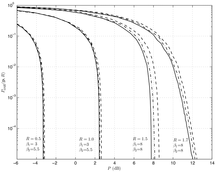
Figure 3: Outage performance of various long-term power allocation schemes for QPSK-input 4-block block-fading channels under Rayleigh fading. The solid-line represents optimal scheme; the dashed line and dashed-dotted line correspondingly represent long-term truncated water-filling ($\mathbf{p}_{\rm lt}^{\rm tw}(\mbox{\boldmath{$\gamma$}})$ with $\beta_{1}$) and its refinement ($\mathbf{p}_{\rm lt}^{\rm ref}(\mbox{\boldmath{$\gamma$}})$ with $\beta_{2}$).

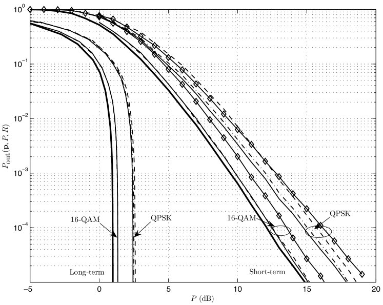
Figure 4: Outage performance of short- and long-term power allocation schemes in a block-fading channel with $B=4$, $R=1$ and Rayleigh fading. Diamonds correspond to uniform allocation, thick solid lines correspond to Gaussian input, thin solid-lines represent optimal schemes; the dashed and dashed-dotted lines represent long-term truncated water-filling ($\mathbf{p}_{\rm lt}^{\rm tw}(\mbox{\boldmath{$\gamma$}})$ with $\beta_{1}=3$) and its corresponding refinement ($\mathbf{p}_{\rm lt}^{\rm ref}(\mbox{\boldmath{$\gamma$}})$ with $\beta_{2}=5.5$), respectively.

VI Conclusion

We considered power allocation schemes for discrete-input block-fading channels with transmitter and receiver CSI under short- and long-term power constraints. We have studied optimal and low-complexity sub-optimal schemes, and have illustrated the corresponding performances, showing that minimal loss is incurred when using the sub-optimal schemes.

References

- [1] L. H. Ozarow, S. Shamai, and A. D. Wyner, “Information theoretic considerations for cellular mobile radio,” IEEE Trans. Veh. Tech., vol. 43, no. 2, pp. 359–378, May 1994.
- [2] E. Biglieri, J. Proakis, and S. Shamai, “Fading channels: Informatic-theoretic and communications aspects,” IEEE Trans. Inf. Theory, vol. 44, no. 6, pp. 2619–2692, Oct. 1998.
- [3] T. M. Cover and J. A. Thomas, Elements of Information Theory, 2nd ed. John Wiley and Sons, 2006.
- [4] G. Caire, G. Taricco, and E. Biglieri, “Optimal power control over fading channels,” IEEE Trans. Inf. Theory, vol. 45, no. 5, pp. 1468–1489, Jul. 2001.
- [5] A. Lozano, A. M. Tulino, and S. Verdú, “Opitmum power allocation for parallel Gaussian channels with arbitrary input distributions,” IEEE Trans. Inf. Theory, vol. 52, no. 7, pp. 3033–3051, Jul. 2006.
- [6] R. Knopp and P. A. Humblet, “On coding for block fading channels,” IEEE Trans. Inf. Theory, vol. 46, no. 1, pp. 189–205, Jan. 2000.
- [7] E. Malkamäki and H. Leib, “Coded diversity on block-fading channels,” IEEE Trans. Inf. Theory, vol. 45, no. 2, pp. 771–781, Mar. 1999.
- [8] A. Guillén i Fàbregas and G. Caire, “Coded modulation in the block-fading channel: Coding theorems and code construction,” IEEE Trans. Inf. Theory, vol. 52, no. 1, pp. 91–114, Jan. 2006.
- [9] K. D. Nguyen, A. Guillén i Fàbregas, and L. K. Rasmussen, “Power allocation for discrete-input delay-limited fading channels,” submitted to IEEE Trans. Inf. Theory. Available at arXiv:0706.2033.
- [10] F. Brännström, L. K. Rasmussen, and A. J. Grant, “Convergence analysis and optimal scheduling for multiple concatenated codes,” IEEE Trans. Inf. Theory, vol. 51, no. 9, pp. 3354–3364, Sep. 2005.