Displacement Detection with a Vibrating RF SQUID: Beating the Standard Linear Limit

Abstract

We study a novel configuration for displacement detection consisting of a nanomechanical resonator coupled to both, a radio frequency superconducting interference device (RF SQUID) and to a superconducting stripline resonator. We employ an adiabatic approximation and rotating wave approximation and calculate the displacement sensitivity. We study the performance of such a displacement detector when the stripline resonator is driven into a region of nonlinear oscillations. In this region the system exhibits noise squeezing in the output signal when homodyne detection is employed for readout. We show that displacement sensitivity of the device in this region may exceed the upper bound imposed upon the sensitivity when operating in the linear region. On the other hand, we find that the high displacement sensitivity is accompanied by a slowing down of the response of the system, resulting in a limited bandwidth.

I Introduction

Resonant detection is a widely employed technique in a variety of applications. A detector belonging to this class typically consists of a resonator, which is characterized by a resonance frequency $\omega_{0}$ and characteristic damping rates. Detection is achieved by coupling the measured physical parameter of interest, denoted as $x$, to the resonator in such a way that $\omega_{0}$ becomes effectively $x$ dependent, that is $\omega_{0}=\omega_{0}\left(x\right)$. In such a configuration $x$ can be measured by externally driving the resonator, and monitoring its response as a function of time by measuring some output signal $X\left(t\right)$. Such a scheme allows a sensitive measurement of the parameter $x$, provided that the average value of $X\left(t\right)$, which is denoted as $X_{0}$, strongly depends on $\omega_{0}$, and provided that $\omega_{0}$, in turn, strongly depends on $x$. These dependencies are characterized by the responsivity factors $R=\left|\partial X_{0}/\partial\omega_{0}\right|$ and $\left|\partial\omega_{0}/\partial x\right|$ respectively. Resonant detection has been employed before for mass detection Ekinci et al. (2004), quantum state readout of a quantum bit Wallraff et al. (2004); Lupascu et al. (2006); Johansson et al. (2006); Lee et al. (2007), detection of gravitational waves Barish and Weiss (1999), and in many other applications.

In general, any detection scheme employed for monitoring the parameter of interest $x$ can be characterized by two important figures of merit. The first is the minimum detectable change in $x$, denoted as $\delta x$. This parameter is determined by the above mentioned responsivity factors, the noise level, which is usually characterized by the spectral density of $X\left(t\right)$, and by the averaging time $\tau$ employed for measuring the output signal $X\left(t\right)$. The second figure of merit is the ring-down time $t_{\mathrm{RD}}$, which is a measure of the detector’s response time to a sudden change in $x$.

In general, the minimum detectable change $\delta x$ is proportional to the square root of the available bandwidth, namely, to $\left(2\pi/\tau\right)^{1/2}$. It is thus convenient to characterize the sensitivity by the minimum detectable change $\delta x$ per square root of bandwidth, which is given by $P_{x}=\delta x/\left(2\pi/\tau\right)^{1/2}$. Under some conditions, which will be discussed below in detail, the smallest possible value of $P_{x}$ is given by Ekinci et al. (2004); Cleland (2005)

$$P_{x}^{\mathrm{SLL}}=\left|\frac{\partial\omega_{0}}{\partial x}\right|^{-1}\left(\frac{\omega_{0}}{2Q}\frac{k_{B}T}{U_{0}}\frac{\hbar\omega_{0}}{2k_{B}T}\coth\frac{\hbar\omega_{0}}{2k_{B}T}\right)^{1/2}\ ,$$ (1)

where $k_{B}T$ is the thermal energy, $U_{0}$ is the energy stored in the resonator, and $Q$ is the quality factor of the resonator. One of the assumptions, which are made in order to derive Eq. (1), is that the response of the resonator is linear. We therefore refer to the value of $P_{x}$ given by Eq. (1) as the standard linear limit (SLL) of resonant detection. Under the same conditions and assumptions, the ring-down time is given by

$$t_{\mathrm{RD}}=\frac{Q}{\omega_{0}}\ .$$ (2)

As can be seen from Eq. (1), sensitivity enhancement can be achieved by increasing $Q$, however, this unavoidably will be accompanied by an undesirable increase in the ring-down time (see Eq. (2)), namely, slowing down the response of the system to changes in $x$. Moreover, Eq. (1) apparently suggests that unlimited reduction in $P_{x}$ can be achieved by increasing $U_{0}$ by means of increasing the drive amplitude. Note however that Eq. (1), which was derived by assuming the case of linear response, is not applicable in the nonlinear region. Thus, in order to characterize the performance of the system when nonlinear oscillations are excited by an intense drive, one has to generalize the analysis by taking nonlinearity into account Lupascu et al. (2006); Wang and Heinz (2002); Santamore et al. (2004a); Cleland (2005); Dykman and Krivoglaz (1984); Buks and Yurke (2006a).

In the present paper we theoretically study a novel configuration for resonant detection of displacement of a nanomechanical resonator Knobel and Cleland (2003); LaHaye et al. (2004), which is coupled to both, a radio frequency superconducting interference device (RF SQUID) and to a superconducting stripline resonator. Similar configurations have been studied recently in Zhou and Mizel (2006); Xue et al. (2007); Buks and Blencowe (2006); Buks et al. (2006); Blencowe and Buks (2007); Wang et al. (2007). We employ an adiabatic approximation and a rotating wave approximation (RWA) to simplify the analysis and calculate the displacement sensitivity. We first consider the case where the response of the stripline resonator is linear and reproduce Eqs. (1) and (2) in this limit. However, we find that the response becomes nonlinear at a relatively low input drive power. Next, we show that $P_{x}$ in the nonlinear region may become significantly smaller than the value given by Eq. (1), exceeding thus the SLL imposed upon the sensitivity when operating in the linear region. On the other hand, we find that the enhanced displacement sensitivity is accompanied by a slowing down of the response of the system, resulting in a limited bandwidth, namely, a ring-down time much longer than the value given by Eq. (2).

II The Device

The device, which is schematically shown in Fig. 1, consists of an RF SQUID inductively coupled to a stripline resonator. The loop of the RF SQUID, which has a self inductance $\Lambda$, is interrupted by a Josephson junction (JJ) having a critical current $I_{c}$ and a capacitance $C_{J}$. A perpendicularly applied magnetic field produces a flux $\Phi_{e}$ threading the loop of the RF SQUID. The stripline resonator is made of two identical stripline sections of length $l/2$ each having inductance $L_{T}$ and capacitance $C_{T}$ per unit length and characteristic impedance $Z_{T}=\sqrt{L_{T}/C_{T}}$. The stripline sections are connected by a doubly clamped beam made of a narrow strip, which is freely suspended and allowed to oscillate mechanically. We assume the case where the fundamental mechanical mode vibrates in the plane of the figure and denote the amplitude of this flexural mode as $x$. Let $m$ be the effective mass of the fundamental mechanical mode, and $\omega_{m}$ its angular resonance frequency. The suspended mechanical beam is assumed to have an inductance $L_{b}$ (independent of $x$) and a negligible capacitance to ground. The coupling between the mechanical resonator and the rest of the system originates from the dependence of the mutual inductance $M$ between the inductor $L_{b}$ and the RF SQUID loop on the mechanical displacement $x$, that is $M=M\left(x\right)$.

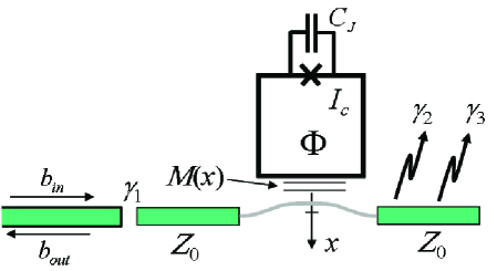
Figure 1: (Color online) The device consists of a nanomechanical resonator coupled to both, a radio frequency superconducting interference device (RF SQUID) and to a superconducting stripline resonator.

II.1 Transmission Line Resonator

The transmission line is assumed to extend from $y=-l/2$ to $y=l/2$, and the lumped inductance $L_{b}$ is located at $y=0$. Consider the case where only the fundamental mode of the resonator is driven. Disregarding all other modes we express the voltage $\mathcal{V}\left(y,t\right)$ and current $\mathcal{I}\left(y,t\right)$ along the transmission line as

$$\mathcal{V}\left(y,t\right) =\left\{\begin{array}[c]{cc}\dot{\varphi}\frac{L_{T}\cos\left[\kappa\left(y+\frac{l}{2}\right)\right]}{\kappa L_{b}\sin\frac{\kappa l}{2}}&y<0\\ -\dot{\varphi}\frac{L_{T}\cos\left[\kappa\left(y-\frac{l}{2}\right)\right]}{\kappa L_{b}\sin\frac{\kappa l}{2}}&y>0\end{array}\right.\;,$$ (5)

$$\mathcal{I}\left(y,t\right) =\left\{\begin{array}[c]{cc}\varphi\frac{\sin\left[\kappa\left(y+\frac{l}{2}\right)\right]}{L_{b}\sin\frac{\kappa l}{2}}&y<0\\ -\varphi\frac{\sin\left[\kappa\left(y-\frac{l}{2}\right)\right]}{L_{b}\sin\frac{\kappa l}{2}}&y>0\end{array}\right.\;,$$ (8)

where $\varphi$ represents the flux in the lumped inductor at $y=0$. The value of $\kappa$ is determined by applying Faraday’s law to the lumped inductor at $y=0$ Blencowe and Buks (2007)

$$\cot\frac{\kappa l}{2}=-\frac{\kappa l}{2}\frac{L_{b}}{L_{T}l}\;.$$ (9)

For the fundamental mode the solution is in the range $\pi\leq\kappa l\leq 2\pi$ (see Fig. 2).

II.2 Inductive Coupling

The total magnetic flux $\Phi$ threading the loop of the RF SQUID is given by

$$\Phi=\Phi_{e}+\Phi_{i}\ ,$$ (10)

where $\Phi_{i}$ represents the flux generated by both, the circulating current in the RF SQUID $I_{s}$ and by the current in the suspended mechanical beam $I_{b}$

$$\Phi_{i}=I_{s}\Lambda+MI_{b}\ ,$$ (11)

where $\Lambda$ is the self inductance of the loop. Similarly, the magnetic flux $\varphi$ in the inductor $L_{b}$ is given by

$$\varphi=I_{b}L_{b}+MI_{s}\ .$$ (12)

Inverting these relations yields

$$I_{s} =\frac{L_{b}\Phi_{i}-M\varphi}{\Lambda L_{b}\left(1-\alpha_{M}^{2}\right)}\ ,$$ (13)

$$I_{b} =\frac{\Lambda\varphi-M\Phi_{i}}{\Lambda L_{b}\left(1-\alpha_{M}^{2}\right)}\ ,$$ (14)

where

$$\alpha_{M}=\frac{M}{\sqrt{\Lambda L_{b}}}\;.$$ (15)

The gauge invariant phase across the Josephson junction $\theta$ is given by

$$\theta=2\pi n-\frac{2\pi\Phi}{\Phi_{0}}\ ,$$ (16)

where $n$ is an integer and $\Phi_{0}=h/2e$ is the flux quantum. We set $n=0$, since observable quantities do not depend on $n$.

II.3 Capacitive and Inductive Energies

Assuming that the only excited mode is the fundamental one, the capacitive energy stored in the stripline resonator is found using Eqs. (5) and (9)

$$\frac{C_{T}}{2}\int_{-l/2}^{l/2}\mathcal{V}^{2}\;\mathrm{d}y=\frac{C_{e}\dot{\varphi}^{2}}{2}\;,$$ (17)

where $C_{e}$, which is given by

$$C_{e}=\frac{C_{T}L_{T}}{2\kappa^{2}\vartheta L_{b}}\;,$$ (18)

represents the effective capacitance of the stripline resonator. The factor $\vartheta$, which is defined by

$$\vartheta=-\frac{\sin\left(\kappa l\right)}{\kappa l+\sin\left(\kappa l\right)}\ ,$$ (19)

can be calculated by solving numerically Eq. (9) (see Fig. 2).

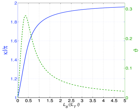
Figure 2: (color online) The factor $\kappa l$ (blue solid line) and $\vartheta$  (green dashed line) calculated using Eq. (9) as a function $L_{b}/L_{T}l$.

Similarly, the inductive energy stored in the resonator, excluding the energy stored in the lumped inductor $L_{b}$ at $y=0$, is found using Eqs. (8) and (9)

$$\frac{L_{T}}{2}\int_{-l/2}^{l/2}\mathcal{I}^{2}\;\mathrm{d}y=\frac{\varphi^{2}}{2L_{e}}\;,$$ (20)

where $L_{e}$, which is given by

$$\frac{1}{L_{e}}=C_{e}\omega_{e}^{2}+\frac{1}{L_{b}}\;,$$ (21)

represents the effective inductance of the stripline resonator excluding the lumped element at $y=0$, and where

$$\omega_{e}=\frac{\kappa}{\sqrt{L_{T}C_{T}}}\;.$$ (22)

The inductive energy stored in the RF SQUID loop and the lumped inductor $L_{b}$ is calculated using Eqs. (13) and (14)

$$\frac{1}{2}\left(\begin{array}[c]{cc}I_{s}&I_{b}\end{array}\right)\left(\begin{array}[c]{cc}\Lambda&M\\ M&L_{b}\end{array}\right)\left(\begin{array}[c]{c}I_{s}\\ I_{b}\end{array}\right)$$ (28)

$$=\frac{\varphi^{2}}{2L_{b}}+\frac{\left(\Phi-\Phi_{e}-\frac{M\varphi}{L_{b}}\right)^{2}}{2\Lambda\left(1-\alpha_{M}^{2}\right)}\;.$$

III Lagrangian and Hamiltonian of the Closed System

Here we derive a Lagrangian for the closed system consisting of the nanomechanical resonator, stripline resonator and the RF SQUID. The effect of damping will be later taken into account by introducing coupling to thermal baths. The Lagrangian of the closed system is expressed as a function of $x$, $\varphi$ and $\Phi$ and their time derivatives (denoted by overdot)

$$\mathcal{L}=\frac{m\dot{x}^{2}}{2}+\frac{C_{e}\dot{\varphi}^{2}}{2}+\frac{C_{J}\dot{\Phi}^{2}}{2}-U_{0}-U_{1}\ ,$$ (30)

where the potential terms are given by

$$U_{0} =\frac{m\omega_{m}^{2}x^{2}}{2}+\frac{C_{e}\omega_{e}^{2}\varphi^{2}}{2}\ ,$$ (31a)

$$U_{1} =\frac{\left(\Phi-\Phi_{e}-\frac{M\varphi}{L_{b}}\right)^{2}}{2\Lambda\left(1-\alpha_{M}^{2}\right)}-\frac{\Phi_{0}I_{c}\cos\frac{2\pi\Phi}{\Phi_{0}}}{2\pi}\ .$$ (31b)

Using Eqs. (10), (13), (14) and (15), the corresponding Euler - Lagrange equations can be expressed as

$$m\ddot{x}+m\omega_{m}^{2}x-I_{s}I_{b}\frac{\mathrm{d}M}{\mathrm{d}x} =0\ ,$$ (32a)

$$C_{e}\ddot{\varphi}+\frac{\varphi}{L_{e}}+I_{b} =0\ ,$$ (32b)

$$C_{J}\ddot{\Phi}+I_{s}+I_{c}\sin\frac{2\pi\Phi}{\Phi_{0}} =0\ .$$ (32c)

The interpretation of these equations of motion is straightforward. Eq. (32a) is Newton’s 2nd law for the mechanical resonator, where the force is composed of the restoring elastic force $$-m\omega_{m}^{2}x M x I_{b} C_{e} L_{e} I_{s} I_{c}\sin\theta C_{J}\dot{V}_{J} V_{J} V_{J}=\left(\Phi_{0}/2\pi\right)\dot{\theta}$$ and the term due to the dependence of on . Eq. (32b) relates the current in the suspended beam with the currents in the effective capacitor and the effective inductor . Eq. (32c) states that the circulating current equals the sum of the current through the JJ and the current through the capacitor, where the voltage across the JJ is given by the second Josephson equation .

The variables canonically conjugate to $x$, $\varphi$ and $\Phi$ are given by $p=m\dot{x}$, $q=C_{e}\dot{\varphi}$ and $Q=C_{J}\dot{\Phi}$ respectively. The Hamiltonian is given by

$$\mathcal{H}=p\dot{x}+q\dot{\varphi}+Q\dot{\Phi}-\mathcal{L}=\mathcal{H}_{0}+\mathcal{H}_{1}\ ,$$ (33)

where

$$\mathcal{H}_{0}=\frac{p^{2}}{2m}+\frac{q^{2}}{2C_{e}}+U_{0}\ ,$$ (34)

$$\mathcal{H}_{1}=\frac{Q^{2}}{2C_{J}}+U_{1}\ .$$ (35)

Quantization is achieved by regarding the variables $\left\{x,p,\varphi,q,\Phi,Q\right\}$ as Hermitian operators satisfying Bose commutation relations.

IV Adiabatic Approximation

As a basis for expanding the general solution we use the eigenvectors of the following Schrödinger equation

$$\mathcal{H}_{1}\left|n\left(x,\varphi\right)\right\rangle=\varepsilon_{n}\left(x,\varphi\right)\left|n\left(x,\varphi\right)\right\rangle\ ,$$ (36)

where $x$ and $\varphi$ are treated here as parameters (rather than degrees of freedom). The local eigen-vectors are assumed to be orthonormal

$$\left\langle m\left(x,\varphi\right)|n\left(x,\varphi\right)\right\rangle=\delta_{nm}\ .$$ (37)

The eigenenergies $\varepsilon_{n}\left(x,\varphi\right)$ and the associated wavefunctions $\varphi_{n}$ are found by solving the following Schrödinger equation

$$\left(-\beta_{C}\frac{\partial^{2}}{\partial\phi^{2}}+u\right)\varphi_{n}=\frac{\varepsilon_{n}}{E_{0}}\varphi_{n}\ .$$ (38)

where

$$u =\frac{\left(\phi-\phi_{0}\right)^{2}}{1-\alpha_{M}^{2}}+2\beta_{L}\cos\phi\ ,$$ (39)

$$\phi =\frac{2\pi\Phi}{\Phi_{0}}-\pi\ ,$$ (40)

$$\phi_{0} =\frac{2\pi\Phi_{e}}{\Phi_{0}}+\frac{2\pi M\left(x\right)\varphi}{\Phi_{0}L_{b}}-\pi\ ,$$ (41)

$$\beta_{L} =\frac{2\pi\Lambda I_{c}}{\Phi_{0}}\ ,$$ (42)

$$\beta_{C} =\frac{2e^{2}}{C_{J}E_{0}}\ ,$$ (43)

$$E_{0} =\frac{\Phi_{0}^{2}}{8\pi^{2}\Lambda}\ .$$ (44)

The total wave function is expanded as

$$\psi=\sum_{n}\xi_{n}\left(x,\varphi,t\right)\left|n\right\rangle\ .$$ (45)

In the adiabatic approximation Moody et al. (1989) the time evolution of the coefficients $\xi_{n}$ is governed by the following set of decoupled equations of motion

$$\left[\mathcal{H}_{0}+\varepsilon_{n}\left(x,\varphi\right)\right]\xi_{n}=i\hbar\dot{\xi}_{n}\ .$$ (46)

Note that in the present case the geometrical vector potential Moody et al. (1989) vanishes since the wavefunctions $\varphi_{n}\left(\phi\right)$ can be chosen to be real. The validity of the adiabatic approximation will be discussed below.

V Two level approximation

In what follows we focus on the case where $\left|\phi_{0}\right|\ll 1$ and $\beta_{L}\left(1-\alpha_{M}^{2}\right)>1$. In this case the adiabatic potential $u\left(\phi\right)$ given by Eq. (39) contains two wells separated by a barrier near $\phi=0$. At low temperatures only the two lowest energy levels contribute. In this limit the local Hamiltonian $\mathcal{H}_{1}$ can be expressed in the basis of the states $\left|\curvearrowleft\right\rangle$ and $\left|\curvearrowright\right\rangle$, representing localized states in the left and right well respectively having opposite circulating currents. In this basis, $\mathcal{H}_{1}$ can be expressed using Pauli’s matrices

$$\mathcal{H}_{1}\dot{=}\eta\phi_{0}\sigma_{z}+\Delta\sigma_{x}\ .$$ (47)

The real parameters $\eta$ and $\Delta$ can be determined by solving numerically the Schrödinger equation (38) Buks and Blencowe (2006). The eigenvectors and eigenenergies are denoted as $\mathcal{H}_{1}\left|\pm\right\rangle=\varepsilon_{\pm}\left|\pm\right\rangle$, where

$$\varepsilon_{\pm}=\pm\sqrt{\eta^{2}\phi_{0}^{2}+\Delta^{2}}\ .$$ (48)

VI Rotating Wave Approximation

Consider the case where $\Phi_{e}=\Phi_{0}/2$, that is

$$\phi_{0}=\frac{2\pi M\left(x\right)\varphi}{\Phi_{0}L_{b}}\;,$$ (49)

and assume that adiabaticity holds and that the RF SQUID remains in its lowest energy state. In this case, as can be seen from Eq. (48), expansion of $\varepsilon_{-}\left(x,\varphi\right)$ yields only even powers of $\varphi$. These even powers of $\varphi$ can be expressed in terms of the annihilation operator

$$A_{e}=\frac{e^{i\omega_{e}t}}{\sqrt{2\hbar}}\left(\sqrt{C_{e}\omega_{e}}\varphi+\frac{i}{\sqrt{C_{e}\omega_{e}}}q\right)\$$ (50)

and its Hermitian conjugate $A_{e}^{{\dagger}}$, yielding terms oscillating at frequencies $2n\omega_{e}$, where $n$ is integer. In the RWA such terms are neglected unless $n=0$ since the effect of the oscillating terms on the dynamics on a time scale much longer than a typical oscillation period is negligibly small Santamore et al. (2004b). Moreover, constant terms in the Hamiltonian are disregarded since they only give rise to a global phase factor. Displacement detection is performed by externally driving the fundamental mode of the stripline resonator. To study the effect of nonlinearity to lowest order we keep terms up to 4th order in $\varphi$. On the other hand, since the mechanical displacement is assumed to be very small, we keep terms up to 1st order only in $x$. Thus, in the RWA the Hamiltonian $\mathcal{H}_{0}+\varepsilon_{-}$ is given by

$$\mathcal{H}_{\mathrm{RWA}}=\hbar\omega_{m}N_{m}+\hbar\omega_{0}\left(x\right)N_{e}+\hbar KN_{e}^{2}\;,$$ (51)

where $N_{m}$ and $N_{e}=A_{e}^{{\dagger}}A_{e}$ are number operators of the mechanical and stripline resonators respectively,

$$K =\frac{3\Delta}{4\hbar}\left(\frac{\eta}{\Delta}\frac{2\pi M_{0}}{\Phi_{0}L_{b}}\sqrt{\frac{\hbar}{2C_{e}\omega_{e}}}\right)^{4}\;,$$ (52)

$$\omega_{0}\left(x\right) =\omega_{e}-\Omega_{2}\left(1+2\frac{\mathrm{d\log}M}{\mathrm{d}x}x\right)\;,$$ (53)

$$\Omega_{2} =\frac{\Delta}{\hbar}\left(\frac{\eta}{\Delta}\frac{2\pi M_{0}}{\Phi_{0}L_{b}}\sqrt{\frac{\hbar}{2C_{e}\omega_{e}}}\right)^{2}\;,$$ (54)

and $M_{0}=M\left(0\right)$.

VII Homodyne Detection

The stripline resonator is weakly coupled (with a coupling constant $\gamma_{1}$) to a semi infinite feedline, which guides the input and output RF signals. To model the effect of dissipation (both linear and nonlinear), we add two fictitious semi infinite transmission lines to the model, which allow energy escape from the resonator. The first transmission line is linearly coupled to the resonator with a coupling constant $\gamma_{2}$, and the second one is nonlinearly coupled with a coupling constant $\gamma_{3}$ Yurke and Buks (2006).

The dependence of $\omega_{0}$ on $x$ can be exploited for displacement detection. This is achieved by exciting the fundamental mode of the stripline resonator by launching into the feedline a monochromatic input pump signal having a real amplitude $b_{in}$ and an angular frequency $\omega_{p}$ close to the resonance frequency $\omega_{0}$. The output signal $c_{out}$ reflected off the resonator is measured using homodyne detection, which is performed by employing a balance mixing with an intense local oscillator having the same frequency as the pump frequency $\omega_{p}$, and an adjustable phase $\phi_{\mathrm{LO}}$. That is, the normalized (with respect to the amplitude of the local oscillator) output signal of the homodyne detector is given by

$$X_{\phi_{\mathrm{LO}}}=c_{out}^{\dagger}e^{-i\phi_{\mathrm{LO}}}+c_{out}e^{i\phi_{\mathrm{LO}}}\ .$$ (55)

To proceed, we employ below some results of Ref. Yurke and Buks (2006), which has studied a similar case of homodyne detection of a driven nonlinear resonator.

VII.1 Equation of Motion

Using the standard method of Gardiner and Collett Gardiner and Collett (1985), and applying a transformation to a reference frame rotating at angular frequency $\omega_{p}$

$$A_{e}=Ce^{-i\omega_{p}t}\ ,$$ (56)

yield the following equation for the operator $C$

$$\frac{\mathrm{d}C}{\mathrm{d}t}+\Theta=F\left(t\right)\ ,$$ (57)

where

$$\Theta\left(C,C^{\dagger}\right) =\left[\gamma+i\left(\omega_{0}-\omega_{p}\right)+\left(iK+\gamma_{3}\right)C^{\dagger}C\right]C$$

$$+i\sqrt{2\gamma_{1}}b_{in}e^{i\phi_{1}}\ ,$$

(58)

$\gamma=\gamma_{1}+\gamma_{2}$, $\phi_{1}$ is the (real) phase shift of transmission from the feedline into the resonator, and $F\left(t\right)$ is a noise term, having a vanishing average $\left\langle F\left(t\right)\right\rangle=0$, and an autocorrelation function, which is determined by assuming that the three semi-infinite transmission lines are at thermal equilibrium at temperatures $T_{1}$, $T_{2}$ and $T_{3}$ respectively.

VII.2 Linearization

Let $C=B+c$, where $B$ is a complex number for which

$$\Theta\left(B,B^{\ast}\right)=0\ ,$$ (59)

namely, $B$ is a steady state solution of Eq. (57) for the noiseless case $F=0$. When the noise term $F$ can be considered as small, one can find an equation of motion for the fluctuation around $B$ by linearizing Eq. (57)

$$\frac{\mathrm{d}c}{\mathrm{d}t}+Wc+Vc^{\dagger}=F\ ,$$ (60)

where

$$W=\left.\frac{\partial\Theta}{\partial C}\right|_{C=B}=\gamma+i\left(\omega_{0}-\omega_{p}\right)+2\left(iK+\gamma_{3}\right)B^{\ast}B\ ,$$ (61)

and

$$V=\left.\frac{\partial\Theta}{\partial C^{\dagger}}\right|_{C=B}=\left(iK+\gamma_{3}\right)B^{2}\ .$$ (62)

VII.3 Onset of Bistability Point

In general, for any fixed value of the driving amplitude $b_{in}$, Eq. (59) can be expressed as a relation between $\left|B\right|^{2}$ and $\omega_{p}$. When $b_{in}$ is sufficiently large the response of the resonator becomes bistable, that is $\left|B\right|^{2}$ becomes a multi-valued function of $\omega_{p}$. The onset of bistability point is defined as the point for which

$$\frac{\partial\omega_{p}}{\partial\left|B\right|^{2}} =0\ ,$$ (63)

$$\frac{\partial^{2}\omega_{p}}{\partial\left(\left|B\right|^{2}\right)^{2}} =0\ .$$ (64)

Such a point occurs only if the nonlinear damping is sufficiently small Yurke and Buks (2006), namely, only when the following condition holds

$$\left|K\right|>\sqrt{3}\gamma_{3}\ .$$ (65)

At the onset of bistability point the drive frequency and amplitude are given by

$$\left(\omega_{p}-\omega_{0}\right)_{c}=\gamma\frac{K}{\left|K\right|}\left[\frac{4\gamma_{3}|K|+\sqrt{3}\left(K^{2}+\gamma_{3}^{2}\right)}{K^{2}-3\gamma_{3}^{2}}\right]\ ,$$ (66)

$$\left(b_{in}\right)_{c}=\frac{8}{3\sqrt{3}}\frac{\gamma^{3}(K^{2}+\gamma_{3}^{2})}{\left(\left|K\right|-\sqrt{3}\gamma_{3}\right)^{3}}\ ,$$ (67)

and the resonator mode amplitude is

$$\left|B\right|_{c}^{2}=\frac{2\gamma}{\sqrt{3}\left(\left|K\right|-\sqrt{3}\gamma_{3}\right)}\ .$$ (68)

VII.4 Ring-Down Time

The solution of the equation of motion (60) can be expressed as Yurke and Buks (2006)

$$c\left(t\right)=\int_{-\infty}^{\infty}\mathrm{d}t^{\prime}G\left(t-t^{\prime}\right)\Gamma\left(t^{\prime}\right)\ ,$$ (69)

where

$$\Gamma\left(t\right)=\frac{\mathrm{d}F\left(t\right)}{dt}+W^{\ast}F\left(t\right)-VF^{\dagger}\left(t\right)\ .$$ (70)

The propagator is given by

$$G\left(t\right)=u\left(t\right)\frac{e^{-\lambda_{0}t}-e^{\lambda_{1}t}}{\lambda_{1}-\lambda_{0}}\ ,$$ (71)

where $u(t)$ is the unit step function, and the Lyapunov exponents $\lambda_{0}$ and $\lambda_{1}$ are the eigenvalues of the homogeneous equation, which satisfy

$$\lambda_{0}+\lambda_{1}=2W^{\prime}\ ,$$ (72)

$$\lambda_{0}\lambda_{1}=|W|^{2}-|V|^{2}\ ,$$ (73)

where $W^{\prime}$ is the real part of $W$. Thus one has

$$\lambda_{0,1}=W^{\prime}\left(1\pm\sqrt{1+\frac{|W|^{2}}{\left(W^{\prime}\right)^{2}}\left(\zeta^{2}-1\right)}\right)\ ,$$ (74)

where

$$\zeta=\left|\frac{V}{W}\right|\ .$$ (75)

We chose to characterize the ring-down time scale as

$$t_{\mathrm{RD}}=\lambda_{0}^{-1}+\lambda_{1}^{-1}=\frac{2W^{\prime}}{\left|W\right|^{2}\left(1-\zeta^{2}\right)}\ .$$ (76)

Note that in the limit $\zeta\rightarrow 1$ slowing down occurs and $t_{\mathrm{RD}}\rightarrow\infty$. This limit corresponds to the case of operating the resonator near a jump point, close to the edge of the bistability region. On the other hand, the limit $\zeta=0$ corresponds to the linear case, for which $t_{\mathrm{RD}}$ at resonance ($\omega_{p}=\omega_{0}$) is given by Eq. (2).

VIII Displacement Sensitivity

Consider a measurement in which $X_{\phi_{\mathrm{LO}}}\left(t\right)$ is monitored in the time interval $\left[0,\tau\right],$ and the average measured value is used to estimate the displacement $x$. Assuming the case where $\tau$ is much longer than the characteristic correlation time of $X_{\phi_{\mathrm{LO}}}\left(t\right)$, one finds that the minimum detectable displacement is given by Ekinci et al. (2004)

$$\delta x=\left|\frac{\partial X_{0}}{\partial x}\right|^{-1}\left(\frac{2\pi}{\tau}\right)^{1/2}P_{X}^{1/2}\left(0\right)\ .$$ (77)

Moreover, using Eq. (53), one finds the minimum detectable displacement per square root of bandwidth, which is defined as $P_{x}=\left(\tau/2\pi\right)^{1/2}\delta x$,  is given by

$$P_{x}=\left|2\Omega_{2}\frac{\mathrm{d\log}M}{\mathrm{d}x}\right|^{-1}R^{-1}P_{X}^{1/2}\left(0\right)\;,$$ (78)

where $R$ is the responsivity with respect to a change in $\omega_{0}$, namely $R=\left|\partial X_{0}/\partial\omega_{0}\right|$. To evaluate $P_{x}$ we calculate below the responsivity $R$ and the spectral density $P_{X}^{1/2}\left(0\right)$ using results, which were obtained in Ref. Yurke and Buks (2006).

VIII.1 Responsivity

In steady state, when input noise is disregarded, the amplitude of the fundamental mode of the stripline resonator is expressed as $Be^{-i\omega_{p}t}$, where the complex number $B$ is found by solving Eq. (59), and the average output signal is expressed as $b_{out}e^{-i\omega_{p}t}$ ($b_{out}$ is in general complex). The amplitude of the output signal in the feedline $b_{out}$ is related to the input signal $b_{in}$ and the mode amplitude $B$ by an input-output relation Gardiner and Collett (1985)

$$b_{out}=b_{in}-i\sqrt{2\gamma_{1}}e^{-i\phi_{1}}B\ .$$ (79)

Consider a small change in the resonance frequency $\delta\omega_{0}$. The resultant change in the steady state mode amplitude $\delta B$ can be calculated using Eq. (59)

$$i\left(\delta\omega_{0}\right)B+W\delta B+V\left(\delta B\right)^{\ast}=0\ .$$ (80)

The solution of this equation together with Eqs. (55) and (79) allows calculating the responsivity

$$R =\frac{2\sqrt{2\gamma_{1}}\left|B\right|}{\left|W\right|\left(1-\zeta^{2}\right)}\left|\sin\left(\phi_{t}+\phi_{C}\right)+\zeta\sin\left(\phi_{t}-\phi_{C}\right)\right|\ ,$$

where

$$\phi_{t} =\frac{2\phi_{\mathrm{LO}}-\phi_{W}+\phi_{V}-2\phi_{1}}{2}\;,$$ (82)

$$\phi_{C} =\frac{2\phi_{B}-\phi_{W}-\phi_{V}-\pi}{2}\;,$$ (83)

$e^{i\phi_{B}}=B/\left|B\right|$, $e^{i\phi_{W}}=W/\left|W\right|$ and $e^{i\phi_{V}}=V/\left|V\right|$.

VIII.2 Spectral Density

The zero frequency spectral density $P_{X}\left(0\right)$ was calculated in Ref. Yurke and Buks (2006)

$$P_{X}\left(0\right) =\left|\frac{2\gamma_{1}\left(1-\zeta e^{2i\phi_{t}}\right)}{\left|W\right|\left(1-\zeta^{2}\right)}-e^{-i\phi_{W}}\right|^{2}\coth\frac{\hbar\omega_{0}}{2k_{B}T_{1}}$$

$$+\frac{\gamma_{2}}{\gamma_{1}}\left|\frac{2\gamma_{1}\left(1-\zeta e^{2i\phi_{t}}\right)}{\left|W\right|\left(1-\zeta^{2}\right)}\right|^{2}\coth\frac{\hbar\omega_{0}}{2k_{B}T_{2}}$$

$$+\frac{2\gamma_{3}\left|B\right|^{2}}{\gamma_{1}}\left|\frac{2\gamma_{1}\left(1-\zeta e^{2i\phi_{t}}\right)}{\left|W\right|\left(1-\zeta^{2}\right)}\right|^{2}\coth\frac{\hbar\omega_{0}}{2k_{B}T_{3}}\ .$$

(84)

VIII.3 The Linear Case

In this case $K=\gamma_{3}=0$, $W=i\left(\omega_{0}-\omega_{p}\right)+\gamma$ and $V=0$, and consequently $\zeta=0$. Thus, the responsivity is given by

$$R=\frac{2\sqrt{2\gamma_{1}}\left|B\right|\left|\sin\left(\phi_{t}+\phi_{C}\right)\right|}{\left|W\right|}\ .$$ (85)

Moreover, for the case where $T_{1}=T_{2}$, Eq. (84) becomes

$$P_{X}\left(0\right)=\coth\frac{\hbar\omega_{0}}{2k_{B}T_{1}}\ .$$ (86)

The largest responsivity is obtained at resonance, namely when $\omega_{p}=\omega_{0}$, and when the homodyne detector measures the phase of oscillations, namely, when $\left|\sin\left(\phi_{t}+\phi_{C}\right)\right|=1$. For this case $P_{x}$ obtains its smallest value, which is denoted as $P_{x0}$, and is given by

$$P_{x0}=\left|2\Omega_{2}\frac{\mathrm{d\log}M}{\mathrm{d}x}\right|^{-1}\left(\frac{\gamma^{2}}{8\gamma_{1}\left|B\right|^{2}}\coth\frac{\hbar\omega_{0}}{2k_{B}T_{1}}\right)^{1/2}\;.$$ (87)

Note that this result coincides with the SLL value $P_{x}^{\mathrm{SLL}}$ given by Eq. (1) provided that the quality factor in Eq. (1) is taken to be given by $Q=2\omega_{0}\gamma_{1}/\gamma^{2}$. That is, $P_{x0}\simeq P_{x}^{\mathrm{SLL}}$ in the limit of strongly overcoupled resonator, namely when the damping of the resonator is dominated by the coupling to the feedline ($\gamma_{1}\simeq\gamma$).

The response of the stripline resonator is approximately linear only when $\left|B\right|$ is much smaller than the critical value corresponding to the onset of nonlinear bistability. Using this critical value $\left|B\right|_{c}$, which is given by Eq. (68), and using Eqs. (52) and (54), one finds that the smallest possible value of $P_{x0}$ in this regime is roughly given by

$$P_{x0,c}\simeq\frac{0.14\left|\frac{\mathrm{d\log}M}{\mathrm{d}x}\right|^{-1}}{\sqrt{\Delta/\hbar}}\sqrt{\frac{\gamma}{\gamma_{1}}\left(1-\frac{\sqrt{3}\gamma_{3}}{\left|K\right|}\right)\coth\frac{\hbar\omega_{0}}{2k_{B}T_{1}}}\;.$$ (88)

VIII.4 The General Case

The minimum detectable displacement per square root of bandwidth in the general case can be written as

$$P_{x}=P_{x}^{\mathrm{SLL}}g\left(\phi_{t}\right)\;,$$ (89)

where

$$g\left(\phi_{t}\right)=\frac{\frac{\left|W\right|}{\gamma}\left[\frac{\left(1-\zeta^{2}\right)^{2}P_{X}\left(0\right)}{\coth\frac{\hbar\omega_{0}}{2k_{B}T_{1}}}\right]^{1/2}}{\left|\sin\left(\phi_{t}+\phi_{C}\right)+\zeta\sin\left(\phi_{t}-\phi_{C}\right)\right|}\;,$$ (90)

and $P_{X}\left(0\right)$ is given by Eq. (84). The function $g\left(\phi_{t}\right)$ is periodic with a period $\pi$. Its minimum value is denoted as $g_{\min}$. Beating the SLL given by Eq. (1) is achieved when $g_{\min}$ is made smaller than unity.

IX Validity of Approximations

In this section we examine the conditions, which are required to justify the approximations made, and determine the range of validity of our results. Clearly, our analysis breaks down if the driving amplitude $b_{in}$ is made sufficiently large. In this case both the adiabatic approximation and the assumption that back-reaction effects are negligibly small will become invalid. The range of validity of the adiabatic approximation is examined below by estimating the rate of Zener transitions. Moreover, we study below the conditions under which back-reaction effects acting back on the mechanical resonator play an important role. Using these results we derive conditions for the validity of the above mentioned approximations. These conditions are then examined for the case where the system is driven to the onset of nonlinear bistability. This analysis allows us to determine whether the device can be operated in the regime of nonlinear bistability, where the effects of bifurcation amplification Wiesenfeld and McNamara (1986); Dykman et al. (1994); Kromer et al. (2000); Savel’ev et al. (2005); Chan and C.Stambaugh (2006); Almog et al. (2006a) and noise squeezing can be exploited Yurke and Buks (2006); Rugar and Grutter (1991); Almog et al. (2006b); Segev et al. (2006a), without, however, violating the adiabatic approximation and without inducing strong back-reaction effects.

IX.1 Adiabatic Condition

As before, consider the case where the externally applied flux is given by $\Phi_{e}=\Phi_{0}/2$, and the stripline resonator is driven close to the onset of nonlinear bistability, where the number of photons approaches the critical value given by Eq. (68), and assume for simplicity the case where $\gamma_{3}\ll\left|K\right|$. Using Refs. Buks and Blencowe (2006); Buks (2006) one finds that adiabaticity holds, namely Zener transitions between adiabatic states are unlikely, provided that

$$\frac{\pi\Delta^{2}}{\eta\hbar\Gamma_{c}}\gtrsim 1\ ,$$ (91)

where

$$\Gamma_{c}=\frac{2\pi M_{0}}{\Phi_{0}L_{b}}\sqrt{\frac{2\hbar\omega_{e}\left|B\right|_{c}^{2}}{C_{e}}}\ .$$ (92)

IX.2 Back Reaction

Back reaction of the driven stripline resonator results in a force noise acting on the mechanical resonator and a renormalization of the mechanical resonance frequency $\omega_{m}$ and the damping rate $\gamma_{m}$ Braginsky and Vyatchanin (2002); Dykman (1978). The renormalized values, denoted as $\omega_{m}^{\mathrm{eff}}$ and $\gamma_{m}^{\mathrm{eff}}$, are expressed using the renormalization factors $R_{\mathrm{f}}$ and $R_{\mathrm{d}}$

$$R_{\mathrm{f}} =\frac{\omega_{m}^{\mathrm{eff}}-\omega_{m}}{\gamma_{m}}\;,$$ (93a)

$$R_{\mathrm{d}} =\frac{\gamma_{m}^{\mathrm{eff}}-\gamma_{m}}{\gamma_{m}}\;,$$ (93b)

which where calculated in Ref. Blencowe and Buks (2007)

$$R_{\mathrm{f}} =\chi_{\mathrm{f}}Q_{m}R_{0}\;,$$ (94a)

$$R_{\mathrm{d}} =\chi_{\mathrm{d}}Q_{m}R_{0}\;,$$ (94b)

where $$Q_{m}=\omega_{m}/\gamma_{m}$$,

$$R_{0}=\frac{8\hbar\Omega_{2}^{2}\left|B\right|^{2}\left(\frac{\mathrm{d\log}M}{\mathrm{d}x}\right)^{2}}{m\omega_{m}^{3}}\;,$$ (95)

$$\chi_{\mathrm{f}} =\frac{\frac{1}{2}\frac{\Delta\omega}{\omega_{m}}\left[\left(\frac{\gamma}{\omega_{m}}\right)^{2}-1+\left(\frac{\Delta\omega}{\omega_{m}}\right)^{2}\right]}{\left[\left(\frac{\gamma}{\omega_{m}}\right)^{2}+\left(1+\frac{\Delta\omega}{\omega_{m}}\right)^{2}\right]\left[\left(\frac{\gamma}{\omega_{m}}\right)^{2}+\left(1-\frac{\Delta\omega}{\omega_{m}}\right)^{2}\right]}\;,$$ (96a)

$$\chi_{\mathrm{d}} =-\frac{\frac{\gamma}{\omega_{m}}\frac{\Delta\omega}{\omega_{m}}}{\left[\left(\frac{\gamma}{\omega_{m}}\right)^{2}+\left(1+\frac{\Delta\omega}{\omega_{m}}\right)^{2}\right]\left[\left(\frac{\gamma}{\omega_{m}}\right)^{2}+\left(1-\frac{\Delta\omega}{\omega_{m}}\right)^{2}\right]}\;,$$ (96b)

and

$$\Delta\omega=\omega_{e}-\Omega_{2}-\omega_{p}\;.$$ (97)

We now wish to examine whether backreaction effects are important when the stripline resonator is driven to the onset of nonlinear bistability. For simplicity we neglect nonlinear damping, that is we take $\gamma_{3}=0$. Using Eqs. (52), (54) and (68), one finds that the value of $R_{0}$ [Eq. (95)] at the onset of nonlinear bistability, which is denoted as $R_{0c}$, is given by

$$R_{0c}=\frac{\gamma}{\omega_{m}}\frac{64\Delta\left(\frac{\mathrm{d\log}M}{\mathrm{d}x}\right)^{2}}{3\sqrt{3}m\omega_{m}^{2}}\;.$$ (98)

It is straightforward to show that $\left|\chi_{\mathrm{f}}\right|<\omega_{m}/\gamma$ and $\left|\chi_{\mathrm{d}}\right|<\omega_{m}/\gamma$ for any value of $\Delta\omega$. Thus, back-reaction can be considered as negligible when

$$\frac{\omega_{m}^{2}}{\gamma\gamma_{m}}R_{0c}\ll 1\;.$$ (99)

X Example

We examine below an example of a device having the following parameters: $Z_{T}=50\operatorname{\Omega}$, $L_{b}/L_{T}l=1$, $\omega_{e}/2\pi=5\operatorname{GHz}$, $\omega_{e}/\gamma=10^{4}$, $\gamma_{2}=0.1\gamma_{1}$, and $\gamma_{3}=0.1K/\sqrt{3}$ for the stripline resonator, $m=10^{-16}\operatorname{kg}$, $\omega_{m}/2\pi=0.01\operatorname{GHz}$, and $\omega_{m}/\gamma_{m}=10^{4}$ for the nanomechanical resonator, $\Lambda=9.1\times 10^{-10}\operatorname{H}$, $C_{J}=0.86\times 10^{-14}\operatorname{F}$, and $I_{c}=0.44\operatorname{\mu A}$ for the RF SQUID, coupling terms $M_{0}/L_{b}=0.005$, $L_{b}/\Lambda=0.25$, $\left|\mathrm{d\log}M/\mathrm{d}x\right|^{-1}=100\operatorname{nm}$, and temperature $T=0.02\operatorname{K}$. These parameters for the stripline resonator Segev et al. (2006b), for the nanomechanical resonator Roukes (2000), and for the RF SQUID Friedman et al. (2000); Koch et al. (1981), are within reach with present day technology.

Using FastHenry simulation program (www.fastfieldsolvers.com) we find that the chosen value of $\Lambda$ corresponds, for example, to a loop made of Al (penetration depth $50\operatorname{nm}$), having a square shape with edge length of $190\operatorname{\mu m}$, line width of $1\operatorname{\mu m}$ and film thickness of $50\operatorname{nm}$. The values of $C_{J}$ and $I_{c}$ correspond to a junction having a plasma frequency of about $25\operatorname{GHz}$.

Using these values one finds $\beta_{L}=1.2$, $\beta_{C}=0.1$, and $E_{0}/\hbar=560\operatorname{GHz}$. The values of $\beta_{L}$, $\beta_{C}$ and $\alpha_{M}$ are employed for calculating numerically the eigenstates of Eq. (38) Buks and Blencowe (2006). From these results one finds the parameters in the two-level approximation of Hamiltonian $\mathcal{H}_{1}$ [Eq. (47)] $\eta=1.2E_{0}$ and $\Delta=0.073E_{0}$, and the nonlinear terms $\Omega_{2}/2\pi=1.3\operatorname{MHz}$ and $K/2\pi=0.19\operatorname{kHz}$.

The validity of the adiabatic approximation is confirmed by evaluating the factor in inequality (91)

$$\frac{\pi\Delta^{2}}{\eta\hbar\Gamma_{c}}=12\ ,$$ (100)

whereas, to confirm that back-reaction effects can be considered as negligible we evaluate the factor in inequality (99)

$$\frac{\omega_{m}^{2}}{\gamma\gamma_{m}}R_{0c}=1.4\times 10^{-4}\;.$$ (101)

Using Eq. (88) we calculate the smallest possible value of $P_{x0}$

$$P_{x0,c}=6.9\times 10^{-14}\frac{\operatorname{m}}{\sqrt{\operatorname{Hz}}}\;.$$ (102)

A significant sensitivity enhancement, however, can be achieved by exploiting nonlinearity. Figure (3) shows the dependence of the mode amplitude $\left|B\right|$, the factor $\zeta$, the reflection coefficient $\left|b_{out}/b_{in}\right|^{2}$, the enhancement factor $g_{\min}$, and the ring-down time $t_{\mathrm{RD}}$ on the pump frequency. Panel (a) represents the nearly linear case for which $b_{in}=0.001\left(b_{in}\right)_{c}$, panel (b) the critical case for which $b_{in}=\left(b_{in}\right)_{c}$, and panel (c) the over-critical case for which $b_{in}=1.5\left(b_{in}\right)_{c}$. As can be clearly seen from Fig. (3) a significant sensitivity enhancement $g_{\min}\ll 1$ can be achieved when driving the resonator close to a jump point. However, in the same region, slowing down occurs, resulting in a long ring-down time $t_{\mathrm{RD}}\gg 2/\gamma$.

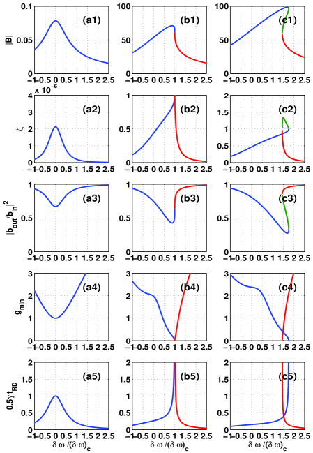
Figure 3: (Color online) Dependence of the mode amplitude $\left|B\right|$, the factor $\zeta$, the reflection coefficient $\left|b_{out}/b_{in}\right|^{2}$, the enhancement factor $g_{\min}$, and the ring-down time $t_{\mathrm{RD}}$ on the pump frequency. Panel (a) represents the nearly linear case for which $b_{in}=0.001\left(b_{in}\right)_{c}$, panel (b) the critical case for which $b_{in}=\left(b_{in}\right)_{c}$, and panel (c) the over-critical case for which $b_{in}=1.5\left(b_{in}\right)_{c}$.

XI Discussion and Conclusions

In the present paper we consider a resonant detection configuration, in which the response of the resonator is measured by monitoring an output signal in the feedline, which is reflected off the resonator. We show that operating in the regime of nonlinear response may allow a significant enhancement in the sensitivity by driving the stripline resonator near a jump point at the edge of the region of bistability. The factor $g_{\min}$, which represents this enhancement, can be made significantly smaller than unity in this limit. However, this result is not general to all resonance detectors. Consider an alternative configuration, in which, instead of measuring an output signal reflected off the resonator, the response is measured by directly homodyning the mode amplitude in the resonator. In the latter case, a similar analysis yields that the enhancement factor $g_{\min}$ cannot be made smaller than $0.5$ Buks and Yurke (2006b). Thus, to take full advantage of nonlinearity, it is advisable to monitor the response of the resonator by measuring a reflected off signal, rather than measuring an internal cavity signal.

As was discussed above, the largest sensitivity enhancement is obtained close to the edge of the region of bistability, where $1-\zeta\ll 1$. On the other hand, in the very same region, the perturbative approach, which we employ to study the response of the stripline resonator, becomes invalid since the fluctuation around steady state, which is assumed to be small, is strongly enhanced due to bifurcation amplification of input noise Yurke and Buks (2006). The integrated spectral density of the fluctuation, which was calculated in Eq. (80) of Ref. Buks and Yurke (2006b) (for the case $T_{1}=T_{2}=T_{3}$), can be employed to determine the range of validity of the perturbative approach

$$\frac{1}{1-\zeta}\coth\frac{\hbar\omega_{0}}{2k_{B}T_{1}}\ll\left|B\right|^{2}\;.$$ (103)

By applying this condition to the case of operating at the onset of bistability point [see panel (b) of Fig. (3)], one finds that the smallest value of $g_{\min}$ in the region where inequality (103) holds is $\simeq 10^{-3}$ for the set of parameters chosen in the above considered example . Thus a significant sensitivity enhancement is achieved even when the region close to the jump, where the perturbative analysis breaks down, is excluded. On the other hand, the perturbative analysis cannot answer the question what is the smallest possible value of $g_{\min}$. Further work is required in order to answer this question and to properly describe the system very close to the edge of the region of bistability, where nonlinear terms of higher orders become important.

In the present paper only the case where back-reaction effects do not play an important role is considered. Thus our results are inapplicable when the displacement sensitivity approaches the value corresponding to zero point motion of the mechanical resonator $\sqrt{\hbar/m\omega_{m}\gamma_{m}}$ ($1.6\times 10^{-15}\operatorname{m}/\sqrt{\operatorname{Hz}}$ for the above considered example), and consequently quantum back-reaction becomes important Caves (1982). Moreover, the results are valid only when inequality (99) is satisfied. To increase the range of applicability of the theory and to study back-reaction effects, a more general approach will be considered in a forthcoming paper Nation et al. (2007).

References

- Ekinci et al. (2004) K. L. Ekinci, Y. T. Yang, and M. L. Roukes, J. Appl. Phys. 95, 2682 (2004).
- Wallraff et al. (2004) A. Wallraff, D. I. Schuster, A. Blais, L. Frunzio, R.-S. Huang, J. Majer, S. Kumar, S. M. Girvin, and R. J. Schoelkopf, Nature 431, 162 (2004).
- Lupascu et al. (2006) A. Lupascu, E. F. C. Driessen, L. Roschier, C. J. P. M. Harmans, and J. E. Mooij, Phys. Rev. Lett. 96, 127003 (2006).
- Johansson et al. (2006) G. Johansson, L. Tornberg, V. S. Shumeiko, and G. Wendin, J. Phys.: Condens. Matter 18, S901 (2006).
- Lee et al. (2007) J. C. Lee, W. D. Oliver, K. K. Berggren, and T. P. Orlando, Phys. Rev. B 75, 144505 (2007).
- Barish and Weiss (1999) B. C. Barish and R. Weiss, Physics Today 52, 44 (1999).
- Cleland (2005) A. N. Cleland, New J. Phys. 7, 235 (2005).
- Wang and Heinz (2002) E. Wang and U. Heinz, Phys. Rev. D 66, 025008 (2002).
- Santamore et al. (2004a) D. H. Santamore, H.-S. Goan, G. J. Milburn, and M. L. Roukes, Phys. Rev. A 70, 052105 (2004a).
- Buks and Yurke (2006a) E. Buks and B. Yurke, Phys. Rev. A 73, 023815 (2006a).
- Dykman and Krivoglaz (1984) M. Dykman and M. Krivoglaz, Soviet Physics Reviews 5, 265 (1984).
- Knobel and Cleland (2003) R. G. Knobel and A. N. Cleland, Nature 424, 291 (2003).
- LaHaye et al. (2004) M. D. LaHaye, O. Buu, B. Camarota, and K. C. Schwab, Science 304, 74 (2004).
- Buks and Blencowe (2006) E. Buks and M. P. Blencowe, Phys. Rev. B 74, 174504 (2006).
- Zhou and Mizel (2006) X. Zhou and A. Mizel, quant-ph/0605017 (2006).
- Xue et al. (2007) F. Xue, Y. Wang, C.P.Sun, H. Okamoto, H. Yamaguchi, and K. Semba, New J. Phys. 9, 35 (2007).
- Buks et al. (2006) E. Buks, E. Segev, S. Zaitsev, B. Abdo, and M. P. Blencowe, arXiv: quant-ph/0610158 (2006).
- Blencowe and Buks (2007) M. P. Blencowe and E. Buks, arXiv: 0704.0457 (2007).
- Wang et al. (2007) Y. D. Wang, K. Semba, and H. Yamaguchi, arXiv:0704.2462 (2007).
- Moody et al. (1989) J. Moody, A. Shapere, and F. Wilczek, in Geometric Phases in Physics, edited by A. Shapere and F. Wilczek (World Scientific Publishing Co., Singapore, 1989), p. 160.
- Santamore et al. (2004b) D. H. Santamore, A. C. Doherty, and M. C. Cross, Phys. Rev. B 70, 144301 (2004b).
- Yurke and Buks (2006) B. Yurke and E. Buks, J. Lightwave Tech. 24, 5054 (2006).
- Gardiner and Collett (1985) C. W. Gardiner and M. J. Collett, Phys. Rev. A 31, 3761 (1985).
- Wiesenfeld and McNamara (1986) K. Wiesenfeld and B. McNamara, Phys. Rev. A 33, 629 (1986).
- Dykman et al. (1994) M. I. Dykman, D. G. Luchinsky, R. Mannella, P. V. E. McClintock, N. D. Stein, and N. G. Stocks, Phys. Rev. E 49, 1198 (1994).
- Kromer et al. (2000) H. Kromer, A. Erbe, A. Tilke, S. Manus, and R. Blick, Europhys. Lett. 50, 101 (2000).
- Savel’ev et al. (2005) S. Savel’ev, A. Rakhmanov, and F. Nori, Phys. Rev. E 72, 056136 (2005).
- Chan and C.Stambaugh (2006) H. B. Chan and C.Stambaugh, arXiv:cond-mat/0603037 (2006).
- Almog et al. (2006a) R. Almog, S. Zaitsev, O. Shtempluck, and E. Buks, Appl. Phys. Lett. 88, 213509 (2006a).
- Rugar and Grutter (1991) D. Rugar and P. Grutter, Phys. Rev. Lett. 67, 699 (1991).
- Almog et al. (2006b) R. Almog, S. Zaitsev, O. Shtempluck, and E. Buks, arXiv: cond-mat/0607055 (2006b), to be published in Phys. Rev. Lett.
- Segev et al. (2006a) E. Segev, B. Abdo, O. Shtempluck, and E. Buks, arXiv: quant-ph/0607262 (2006a), to be published in Phys. Lett. A.
- Buks (2006) E. Buks, J. Opt. Soc. Am. B 23, 628 (2006).
- Braginsky and Vyatchanin (2002) V. B. Braginsky and S. P. Vyatchanin, Phys. Lett. A 293, 228 (2002).
- Dykman (1978) M. Dykman, Soviet Physics - Solid State 20, 1306 (1978).
- Segev et al. (2006b) E. Segev, B. Abdo, O. Shtempluck, and E. Buks, IEEE Trans. Appl. Supercond. 16, 1943 (2006b).
- Roukes (2000) M. L. Roukes, arXiv: cond-mat/0008187 (2000).
- Friedman et al. (2000) J. R. Friedman, V. Patel, W. Chen, S. K. Tolpygo, and J. E. Lukens, Nature 406, 43 (2000).
- Koch et al. (1981) R. H. Koch, D. J. V. Harlingen, and J. Clarke, Phys. Rev. Lett. 47, 1216 (1981).
- Buks and Yurke (2006b) E. Buks and B. Yurke, Phys. Rev. E 74, 046619 (2006b).
- Caves (1982) C. M. Caves, Phys. Rev. D 26, 1817 (1982).
- Nation et al. (2007) P. Nation, M. P. Blencowe, and E. Buks (2007), in progress.