The stability of poloidal magnetic fields in rotating stars

The stability of large-scale magnetic fields in rotating stars is explored, using 3D numerical hydrodynamics to follow the evolution of an initial poloidal field. It is found that the field is subject to an instability, located initially on the magnetic equator, whereby the gas is displaced in a direction parallel to the magnetic axis. If the magnetic axis is parallel to the rotation axis, the rotation does not affect the initial linear growth of the instability, but does restrict the growth of the instability outside of the equatorial zone. The magnetic energy decays on a timescale which is a function of the Alfvén crossing time and the rotation speed, but short compared to any evolutionary timescale. No evidence is found for a possible stable end state to evolve from an initial axisymmetric poloidal field. The field of an oblique rotator is similarly unstable, in both cases regardless of the rotation speed.

1 Introduction

The question of the stability of large-scale fields in stars has accompanied the historical development of magnetohydrodynamics (MHD) right from the beginning. Over the same period, large-scale magnetic fields have been detected in a variety of stars – since their discovery in Ap stars (Babcock (1947)) they have also been observed (or their presence inferred) in white dwarfs, neutron stars, upper-main-sequence stars, central stars of planetary nebulae, etc. (e.g. Kemp et al. (1970), Angel et al. (1974), Henrichs et al. (2003), Jordan et al. (2005)). It seems implausible that these fields can be regenerated by a convective dynamo. This is because, in contrast to solar-type main sequence stars, these stars have either no significant convective zone, in the case of white dwarfs and neutron stars, or just a small convective core, in the case of upper-main-sequence stars. Any field produced in this convective core would struggle to rise to the surface on a sensible timescale (see, e.g. Moss (2001)). There is also the lack of one hallmark of dynamo activity – the correlation between rotation rate and magnetic field strength found in solar-type and some other stars (Borra & Landstreet (1980), Mathys et al. (1997)). For this reason there has been great interest in finding some magnetic field configuration which is stable on a sufficiently long timescale and which can therefore persist without recourse to a continuous generative mechanism.

By means of the following non-rigorous argument, one can see that it should be possible to construct a magnetic field in equilibrium, i.e. where the Lorentz, gravity and pressure forces cancel everywhere. Because of the zero-divergence constraint, the magnetic field, and therefore the Lorentz force, has two degrees of freedom. Luckily, we have two degrees of freedom in making adjustments to the thermodynamic state of the star, e.g. to the temperature and pressure fields. In this way, the net force on every fluid element can be brought to zero.

The next question is that of the stability of an equilibrium to an arbitrary perturbation. Tayler (1973) examined purely toroidal fields (i.e. having only the azimuthal component $B_{\phi}$) in non-rotating stars, finding necessary and sufficient conditions for stability. It is generally supposed that these stability conditions would be impossible to satisfy at every point in the star. The resulting instability, which is global in the azimuthal direction, will grow on the timescale given by the time taken for an Alfvén wave to travel across the star ($\sim 10$ years in a $1M_{\odot}$, $1R_{\odot}$ star with a field of $1$ kilogauss). Some properties of this instability have now been analysed numerically by Braithwaite (2006). It has also been shown that any purely poloidal field (i.e. having only components $B_{r}$ and $B_{\theta}$ in spherical polars; one example of a poloidal field is illustrated on the right-hand-side of fig. 1) is also unstable in a non-rotating star (Markey & Tayler 1973, 1974, Wright (1973), Braithwaite & Spruit (2006)). At least in a non-rotating setup, a stable field had therefore to be of a mixed toroidal-poloidal form, and Wright (1973) suggested that a toroidal field could indeed be stabilised by adding a poloidal field of comparable strength.

These previous studies described above worked by taking various field configurations and examining their stability, by either analytic or, in the case of Braithwaite & Spruit (2006), numerical means. A different approach is to take an arbitrary magnetic field, which one assumes will be not only not in stable equilibrium but not in any equilibrium, and to follow its evolution in time, to see if it eventually finds a stable equilibrium on its own. A study of this kind has now been done: following the evolution of an arbitrary initial field using numerical MHD, a stable equilibrium was found (Braithwaite & Spruit (2004), Braithwaite & Nordlund (2006)). This stable field is of a mixed poloidal-toroidal twisted-torus shape. Moreover, this was the only stable equilibrium found, starting from various different initial magnetic fields. It is illustrated qualitatively on the left-hand-side of fig. 1.

It seems likely therefore that in a non-rotating star, there is only one possible stable magnetic field configuration. The question of what is stable and unstable in a rotating star, however, has historically received less attention, largely because of the increased complexity of the problem. A useful method of demonstrating stability in a non-rotating system is to show that for all arbitrary perturbations, the energy of the system increases. If even only one perturbation can be found for which the energy decreases, the system is unstable. Unfortunately, this method does not work in a rotating system. To understand why, imagine trying to push a ball off the top of a hill. The potential energy of the ball falls as it moves further from the summit, and one could conclude that the equilibrium at the top of the hill is an unstable one. However, a Coriolis force will cause the ball to move in a curve and eventually to come back to where it started (on an idealised hill without friction).

Frieman & Rotenberg (1960) demonstrated that solid-body rotation would not have a significant effect on hydromagnetic instabilities unless the rotation velocity was at least comparable to the hydromagnetic velocity. This is the case for some, but not all, magnetic stars. [Indeed, within each group, including neutron stars, white dwarfs and upper main sequence stars, there are some slow rotators and some fast rotators; for instance, some neutron stars (magnetars) have an Alfvén crossing time and rotation timescale ($\Omega^{-1}$) of $0.1$s and $1$s respectively, while a typical radio pulsar might have corresponding timescales of $100$s and $0.1$s.] Pitts & Tayler (1985) looked at these faster rotating stars, concluding that instabilities in toroidal fields are unlikely to be stabilised entirely, rather the growth rate is merely reduced by a factor roughly equal to the ratio of rotation and hydromagnetic velocities, and that the instabilities in poloidal fields are unlikely to be suppressed, unless (perhaps) the magnetic axis is inclined at a large angle to the rotation axis.

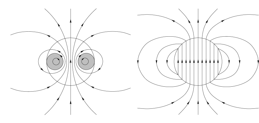
Figure 1: Two magnetic field configurations. On the left, the mixed poloidal-toroidal field (shading in diagram represents toroidal field) shown to be stable in a non-rotating star (Braithwaite & Spruit (2004)). On the right, a purely poloidal field. All purely poloidal fields are known to be unstable in a non-rotating star.

More recently, Geppert & Rheinhardt (2006) have used numerical MHD to look at the stability of poloidal fields in rotating stars, finding that if the star is rotating quickly enough, and if the field is roughly aligned to the rotation axis, the instability is suppressed. This is at odds with the results presented here; this difference is discussed in section 5.

In this study, I use numerical methods to investigate the stability of poloidal fields in rotating stars. The paper is organised as follows. In the next section, I review the form of the instability expected to be present in non-rotating stars. The model used in the investigation is outlined in section 3, as well as some of the technical and computational details. I present the results in section 4, and finish with a summary of the conclusions and a discussion of their implications in section 5.

2 The form of the instability in poloidal fields

In the results obtained so far with analytic methods, a distinction has been made between poloidal fields where some of the field lines are closed within the star and poloidal fields where all field lines pass through the stellar surface. However, the results (in the non-rotating case) have been the same: an instability whose growth rate is comparable to the Alfvén crossing time.

The cause of the instability (in at least the latter type of poloidal field) can be understood intuitively by means of the following line of reasoning (Flowers & Ruderman (1977)). Imagine the star as being composed of two solid halves, each containing a frozen-in magnetic field, and free to rotate about a common axis. The star now resembles two parallel bar magnets. The bar magnets will of course rotate until the north pole of one is next to the south pole of the other, and the star can do exactly the same. Thinking of this in energy terms, the magnetic energy stored in the star is unchanged but the energy in the atmosphere has fallen, providing energy to drive the instability. One difference between the bar magnets and the star is that while the bar magnets are only unstable to one mode of the instability (i.e. the azimuthal wavenumber $m=2$), the star is subject also to instability at higher wavenumbers.

Even when some of the field lines are closed within the star, the bar magnets analogy is still of some use, since rotating one half of the star by $180^{\circ}$ will still result in a decrease in magnetic energy outside of the star. Theoretically is it possible that all field lines are closed within the star, (it seems unlikely that a star born out of a molecular cloud could be completely cut off from the cloud’s field, but in some stars there could plausibly be a mechanism on the stellar surface to bury the magnetic field entirely from view as is sometimes described in models of accreting neutron stars,) and in this case (as in the other two cases just described) it is helpful to think in terms of the magnetic field loops exerting pressure on each other and there being a tendency for them to slip out of the equilibrium position (or in other words, be pushed out by pressure from the neighbours). Since the movement of these loops is restricted in the radial direction by the stable stratification of the star, they move in a direction parallel to the magnetic axis. This is illustrated in fig. 2.

It has been shown that a system of two bar magnets can indeed be stabilised by rotation (see Jones et al. (1997)). However, there is reason to believe that the analogy between bar magnets and stars does not hold here, because a star is fluid and has more degrees of freedom. More precisely, the magnetic field loops described in the last paragraph move parallel to the magnetic axis, and if this coincides with the rotation axis, the Coriolis force will have no effect, at least in the limit of small displacements.

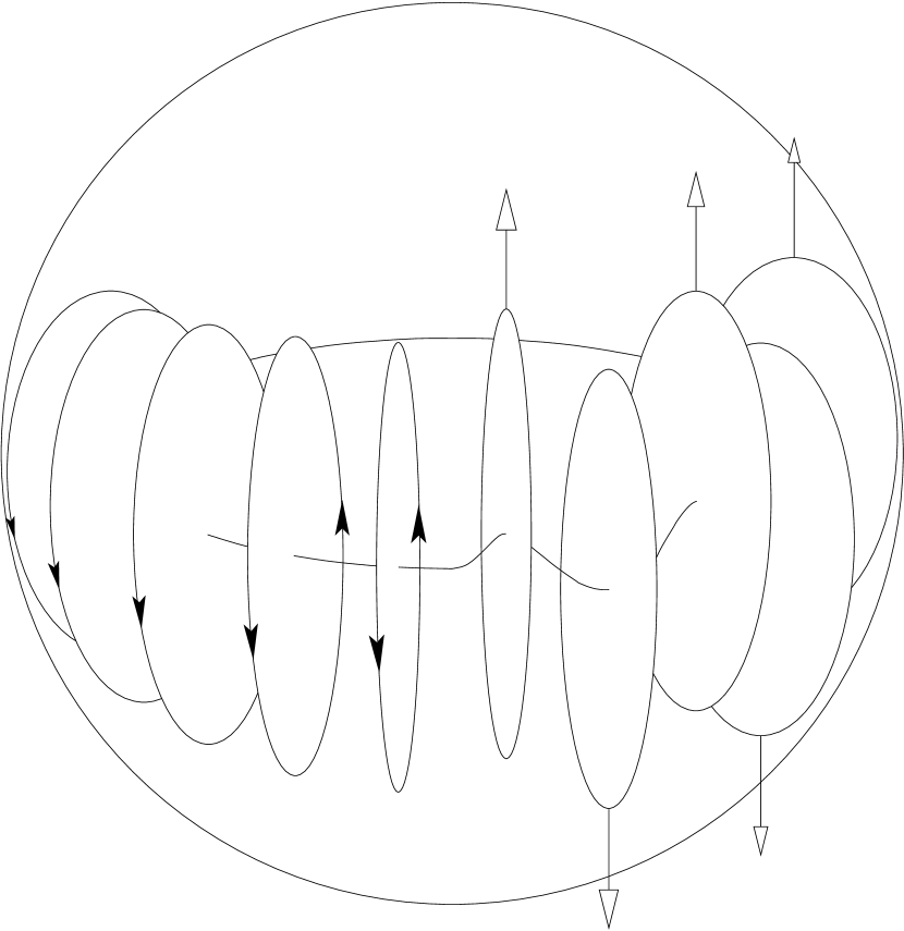
Figure 2: Loops of poloidal magnetic field in a star. The left-hand-side of the star is in equilibrium. On the right, the form of the instability is shown – displacements are essentially parallel to the magnetic axis and perpendicular to gravity. For clarity, a line is drawn connecting the centres of each field loop.

3 The numerical model

The numerical model used is identical to that described in Braithwaite & Nordlund (2006), to which the reader is referred for a fuller account. The only differences here are the initial magnetic field and the rotation, which are described in sections 3.1 and 3.2.

We use a three-dimensional MHD code developed by Nordlund & Galsgaard (1995), which uses Cartesian coordinates, sixth-order spatial derivatives and the third-order predictor-corrector time-stepping routine of Hyman (1979), The code has a numerical diffusion scheme which is designed to damp structure on scales near the Nyquist frequency whilst preserving structure on well-resolved length scales. In the simulations presented here, a resolution of $72^{3}$ was used. Tests were also performed at a lower resolution of $48^{3}$, and the results were not found to differ significantly, except at high azimuthal wavenumbers near the Nyquist frequency, as one would expect.

The fluid obeys the ideal gas equation of state $p=\rho RT$, and an energy equation is solved along with the mass and momentum conservation equations. The star is modelled as a self-gravitating ball of gas, stably stratified (we use a polytropic of index n=3), embedded in a computational cube of side $4.5R_{\ast}$ where $R_{\ast}$ is the radius of the star. Surrounding the star is a hot atmosphere of low electrical conductivity – a physical magnetic diffusion term was added, in contrast to the low-level artificial scheme already present. This causes the field in the atmosphere to relax to a potential (curl-free) field over a timescale of the order of $R_{\ast}^{2}/\eta\sim 30\Omega^{-1}_{\rm crit}$ (where $\Omega_{\rm crit}$ is the break-up spin of the star, roughly equal to the reciprocal of the sound crossing time). Boundary conditions are periodic.

3.1 Rotation

Instead of beginning the simulations with the star rotating inside the computational box, we transfer to the rotating frame by adding a Coriolis force. This avoids having shear flows at the boundaries, which would be problematic in any geometry but particularly so in a square computational box.

A strict transformation to the rotating frame would of course also require a centrifugal force, but I have not included this for the following three reasons. Firstly, it is not thought that the centrifugal force affects the stability of a magnetic field configuration, since, being a curl-free force, it can be balanced by pressure forces, resulting merely in an adjustment to the shape of the star, i.e. rotational oblateness. Secondly, comparison with analytic results will be more direct, as none of the earlier works included the centrifugal term. Thirdly, a practical reason – producing an initial equilibrium is easier with a spherical star (although it can in principle be done in a flattened star). Eventually, one might want to add a centrifugal force to look at phenomena unique to stars rotating close to break up.

3.2 Initial conditions

The non-magnetic aspect of the initial conditions is identical to that described in detail in section 5 of Braithwaite & Nordlund (2006). In the present study, we would like to create an equilibrium poloidal magnetic field to start the simulation with. There are several configurations to choose, and fortunately it is not expected that our choice will affect the overall result (but this is confirmed later – see section 4.3).

Figure 3: The initial equilibrium magnetic field, of the Roberts (1981) form. The surface of the star is represented by the thick line.

A first step towards finding an equilibrium field will be to find a configuration where the Lorentz force $\nabla\times\mathbf{B}\times\mathbf{B}$ is curl-free and can therefore be balanced more easily by the pressure force. One example of such a field is (Roberts (1981)):

$$\mathbf{B}_{r} = \frac{B_{0}}{2}\cos\theta(5-3a^{2}),$$

$$\mathbf{B}_{\phi} = 0,$$

$$\mathbf{B}_{\theta} = \frac{B_{0}}{2}\sin\theta(6a^{2}-5)$$

inside the star, and

$$\mathbf{B}_{r} = \frac{B_{0}\cos\theta}{a^{3}},$$

$$\mathbf{B}_{\phi} = 0,$$

$$\mathbf{B}_{\theta} = \frac{B_{0}\sin\theta}{2a^{3}}$$

outside the star, expressed in spherical coordinates where $a=r/R_{\ast}$, with $R_{\ast}$ being the stellar radius, and where $B_{0}$ is the field strength at the surface of the star at the magnetic poles. We shall use this configuration in the simulations. [This is the same field configuration as that used by Geppert & Rheinhardt (2006).] The field lines of this configuration are plotted in fig. 3. However, simply adding this field to the star will not produce an equilibrium. To reach a numerical equilibrium, the simulation is run for a short time whilst the magnetic field is held fixed, allowing the pressure (and density) field(s) in the star to adjust to the Lorentz force.

3.3 Units and timescales

The maximum angular velocity at which a star can rotate without breaking up is given by $\Omega_{\rm crit}=\sqrt{GM_{\ast}/R_{\ast}^{3}}$ (where $M_{\ast}$ and $R_{\ast}$ are the stellar mass and radius). The inverse of this, $\Omega_{\rm crit}^{-1}$ – which is roughly equal to the sound-crossing time – I use as the time unit in this paper. The mass and radius of the star are used as the mass and length units, the results in section 4 being expressed in this system of units. In these dimensionless units, the thermal energy of the star is equal to $0.55$ and the magnetic energy used here is initially $1.3\times 10^{-3}$.

The relevant frequencies (or inverse timescales) are the angular velocity of the star $\Omega$ (which obviously cannot exceed $1$ as this is the break-up velocity) and the Alfvén frequency $\omega_{\rm A}$, which is an average Alfvén speed divided by the stellar radius and is given by $\omega_{\rm A}=\sqrt{2E_{\rm mag}/M_{\ast}}/R_{\ast}$, where $E_{\rm mag}$ is the total magnetic energy of the star. We are expecting the growth rate of any instability present to be proportional and comparable to $\omega_{\rm A}$, or perhaps lower in the case of fast rotation (Pitts & Tayler (1985)).

From observations of real stars we know that almost always $\omega_{\rm A}\ll 1$, and that $\Omega$ may have any value from $10^{-8}$ (e.g. some white dwarfs) to $0.9$ or higher (e.g. Vega). In the simulations presented here, $\omega_{\rm A}=0.05$, which is high enough to be computationally practical whilst still satisfying the condition $\omega_{\rm A}\ll 1$ and making both the $\omega_{\rm A}\ll\Omega$ and $\omega_{\rm A}\gg\Omega$ regimes accessible.

4 Results

First I shall describe simulations with parallel rotation and magnetic axes ($\chi=0$), before coming to oblique rotators in section 4.2.

4.1 Aligned rotator with $\omega_{\rm A}=0.05$

To begin with, I run simulations with $\omega_{\rm A}=0.05$ and a variety of angular velocities $\Omega=0,0.125,0.25,0.5$ and $1$. In fig. 4 the radial component of the magnetic field $B_{r}$ on the surface of the star is plotted at different timesteps for two of the runs, $\Omega=0$ and $0.5$. Looking first at the left column of the figure, one can see the progress of the instability in the non-rotating case: at first there is a movement of gas both upwards and downwards, confined to the equatorial zone, and the instability then spreads to the whole star, the field losing its overall orientation. In the rotating case ($\Omega=10\omega_{\rm A}$) we see that the instability is at first not affected, but that instead of spreading unhindered to the whole star, it stays mainly in the equatorial zone, the amplitude falling towards the poles. It seems then that rotation does not stabilise the magnetic field, but merely restricts its growth.

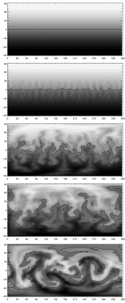
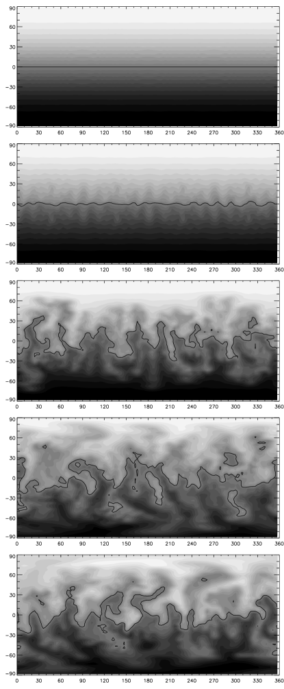
Figure 4: Maps of the radial component of the magnetic field, $B_{r}$, on the surface of the star. White indicates positive $B_{r}$ and black negative; the $B_{r}=0$ line is also plotted. Longitude on the horizontal axis and Latitude on the vertical. Maps are plotted from two runs, with $\Omega=0$ on the left and $\Omega=0.5$ on the right, at five times $t=0,40.1,64.9,92.8$ and $154.7$. Rotation has no obvious effect on the linear development of the instability, but at later times the rotation does restrict the instability away from the equator.

We shall now look at the linear growth phase of the instability in more detail. To do this, I first calculate the azimuthal Fourier components of the vertical component of the velocity field $v_{z}$ (in cylindrical coordinates). The other components of the velocity field, or indeed of the magnetic field, can also be examined in this way, but $v_{z}$ is the most suitable because the amplitudes are higher. The amplitude of the $m=13$ mode in the $\varpi$-$z$ plane at a time $t=30.4$ in the $\Omega=0.5$ case (before the second plot on the right of fig. 4) is plotted in fig. 5. This confirms our original picture of the instability as being strongest on the magnetic equator.

Figure 5: Contour plot of the amplitude of the vertical component of the velocity field $v_{z}$ in the $\varpi$-$z$ plane (on the horizontal and vertical axes respectively), for the $m=13$ mode at time $t=30.3$ in the case where $\Omega=0.5$. The dashed line represents the surface of the star. It can be seen that the instability is located on the equator of the star, just below the surface.

We can now integrate these azimuthal modes over an area in the $\varpi$-$z$ plane (from $\varpi=0.6$ to $0.9$ and from $z=-0.15$ to $+0.15$, i.e. where the velocity field is strongest), and the resulting amplitudes of five Fourier modes are plotted in fig. 6, along with their associated time derivatives, for the $\Omega=0$ and $0.5$ cases. It can be seen that after some initial fluctuations, the modes grow fairly steadily. All of the modes grow at roughly the same growth rate, around $0.28$ or $5.6\omega_{\rm A}$, with just the $m=5$ mode lagging behind; a little higher than we were expecting, but it is safe to assume that this is simply to do with our definition of $\omega_{\rm A}$: in the part of the star where the instability is strongest, the Alfvén velocity is higher than the average for the whole star. This is because the density is much lower there (by a factor $\sim 1000$) than in the centre of the star, more than making up for the somewhat weaker magnetic field. More importantly, there is very little difference between the non-rotating and rotating cases in this linear growth phase.

Figure 6: Above, amplitudes of five azimuthal modes for the non-rotating case (above left) and for the $\Omega=0.5$ case (above right). Aligned ($\chi=0$) case, Roberts initial field. These plots end at the time when the instability growth becomes non-linear. Below, the time derivatives of these log amplitudes, i.e. the growth rates of the various $m$ modes. It is clear that rotation has little effect on the linear stage.

Figure 7: Total magnetic energy against time for runs with different values of $\Omega$: $0,0.125,0.25,0.5$ and $1$. It can be seen that rotation merely slows the decay rather than stopping it altogether. Aligned ($\chi=0$) case, Roberts initial field.

Figure 8: Rate of decay of magnetic energy against time for $\Omega=0,0.125,0.25,0.5$ and $1$, i.e. (minus) the time derivative of (log) fig. 7.

Rotation therefore only affects the non-linear development of the instability, and it is this which is most interesting for applications in astrophysics because it is during the non-linear phase that the magnetic energy is lost. In fig. 7 the total magnetic energy in the star is plotted against time, for the five runs with $\Omega=0,0.125,0.25,0.5$ and $1$. One can see that in all cases, most of the energy is destroyed by the instability. However, it is not clear from this graph alone that the total magnetic energy is heading to zero. The rate at which magnetic energy is being lost, $-(1/E_{\rm mag})dE_{\rm mag}/dt$ is plotted in fig. 8, showing that the rate of energy loss reaches a peak and then declines. However as the instability, and therefore the rate of energy loss, operate at a speed dependent on the Alfvén frequency, we should of course expect the magnetic decay rate to decline.

It is possible to quantify the containment of the instability to the equatorial region by defining a new quantity as the fraction of the stellar surface over which the sign of $B_{\rm r}$ is not the same as at $t=0$. Evolution to a completely random field distribution would give a value around $0.5$, while a configuration like that in the lower-right of fig. 4 would have a smaller value. Fig. 9 is a graph of this quantity against time for the five runs with different angular velocities. It can be seen that in the four rotating runs, the value sinks gradually back down to zero. This is because the Alfvén frequency $\omega_{\rm A}$ falls, also falling in relation to the angular velocity $\Omega$. This in turn causes the more unstable region to shrink towards the magnetic equator, so there is the double effect of energy being lost both more slowly and in a smaller volume. Eventually, we would expect the quantity plotted in fig. 4 to fall to zero as the total magnetic energy falls to zero. Also, note that in numerical simulations, in practice the rate of energy loss from the instability will eventually fall below the energy loss rate from Ohmic dissipation of the global magnetic field, and the instability will no longer have much effect on the field’s evolution. In a real star, with much lower magnetic diffusivity than is accessible in simulations, this end-state will be reached only when the field has become vanishingly weak.

Figure 9: The fraction of the surface of the star where the radial component of the magnetic field $B_{r}$ is of opposite sign to that initially, for five runs with different rotation speeds. In the non-rotating case, this quantity stays close to $0.5$, but in all of the other cases, it sinks slowly back down to zero after the initial rise. This is because the instability is largely confined to a volume near the equatorial plane, and as the magnetic energy is destroyed there, $\omega_{\rm A}$ falls, and the thickness of this volume falls too.

Figs. 10 and 11 show azimuthal averages of the magnetic energy density and current density at different times in the non-rotating and rotating cases. It can be seen that the region of strongest field shrinks in both cases towards the centre of the star, and that the region where the magnetic energy is being lost (where the current density is high) is restricted in the rotating case to a ring around the equator. It is also possible to look at the energy balance between the equatorial region and the rest of the star. For the rotating case $\Omega=1$, figs. 12 and 13 show magnetic energy and integrated current density plotted against time, divided into two parts: the equatorial zone (defined as $-0.3R_{\ast}<z<0.3R_{\ast}$) and the rest of the star. These graphs show that although the equatorial zone accounts for the majority of magnetic energy loss, the energy outside of this zone decays just as fast or faster as inside the equatorial zone. From this we may infer the presence of some kind of transport process carrying energy from the polar regions towards the equator.

Figure 10: An azimuthal average in the $\varpi-z$ plane of the magnetic energy density $B^{2}/8\pi$, at time $t=0$ (left), at time $t=926$ in the $\Omega=0$ case (centre), and at time $t=926$ in the $\Omega=1$ case (right). The dotted line represents the stellar surface. Aligned ($\chi=0$) case, Roberts initial field.

Figure 11: An azimuthal average in the $\varpi-z$ plane of the current density $J^{2}$, at time $t=0$ (left), at time $t=926$ in the $\Omega=0$ case (centre), and at time $t=926$ in the $\Omega=1$ case (right). The dotted line represents the stellar surface. Aligned ($\chi=0$) case, Roberts initial field.

Figure 12: Magnetic energy inside the star, in two components: the volume within $0.3R_{\ast}$ (solid line) of the equator (i.e. $-0.3R_{\ast}<z<0.3R_{\ast}$) and the rest of the star (dotted line). Aligned ($\chi=0$) case, Roberts initial field, $\Omega=1$.

Figure 13: Integrated current density inside the star, in two components: the volume within $0.3R_{\ast}$ (solid line) of the equator (i.e. $-0.3R_{\ast}<z<0.3R_{\ast}$) and the rest of the star (dotted line). Aligned ($\chi=0$) case, Roberts initial field, $\Omega=1$.

4.2 The oblique rotator

If $\chi$ is the angle between the rotation axis and magnetic axis, we have seen that if $\chi=0$ the rotation is not able to stabilise the magnetic field. We shall now generalise to $\chi\not=0$. Identical simulations were run to the $\Omega=0.5$ run described in section 4.1, but with $\chi=45^{\circ}$ and $90^{\circ}$. The magnetic energy in these runs (along with the original $\chi=0^{\circ}$ run) is plotted in fig. 14. It is clear that the field is still not stabilised – in fact, the magnetic energy falls slightly more quickly than when the two axes are aligned.

Figure 14: Total magnetic energy against time for runs with different values of $\chi$: $0^{\circ},45^{\circ}$ and $90^{\circ}$. The magnetic field is unstable, regardless of the relative alignment of the magnetic and rotation axes. Roberts initial field, with $\Omega=0.5$.

4.3 Other poloidal field configurations

It is now necessary to repeat these simulations with some different poloidal field configurations, in case the field used so far is special in some way. We shall use two alternative poloidal fields. First, a field (the poloidal component of a field suggested by Kamchatnov, 1982; denoted as type A in figs. 15 and 16) given by:

$$\mathbf{B}_{r} = \frac{B_{0}\cos{\theta}}{(1+a^{2})^{2}},$$

$$\mathbf{B}_{\phi} = 0,$$

$$\mathbf{B}_{\theta} = \frac{B_{0}\sin{\theta}(a^{2}-1)}{(1+a^{2})^{3}}$$

where $a=r/R_{\rm m}$, with $R_{\rm m}$ being some radius less than the radius of the star. In the following simulations, I use $R_{\rm m}=0.25R_{\ast}$. Secondly, I use a magnetic field uniform in strength and direction inside the star attached to a curl-free field outside the star, as on the right-hand-side of fig. 1 (denoted as type B in figs. 15 and 16). This is the field configuration used to study the non-rotating case by Braithwaite & Spruit (2006). These two configurations were picked for the following reasons. The first of these fields has the property that most of the field lines close inside the star, in contrast to the field used up to now, where most of the field lines go through the surface of the star. Moreover, it is found that together with the toroidal component, as proposed by Kamchatnov, it can be stable (in conjunction with the right velocity field) and has basically the same form as the stable fields found in Braithwaite & Nordlund (2006). Indeed, simulations using the Kamchatnov field (with both poloidal and toroidal components) as the initial field do appear to show that the field is stable in a non-rotating star, or at least that the field quickly relaxes into a very similar-looking stable state. [This will be described in more detail in a forthcoming paper.] Note that the field as given by the equations above does contain a non-potential field in the atmosphere, which will quickly relax to curl-free at the beginning of the simulation. The second field was chosen because of its simple structure, because all field lines close outside the star, and because it has already been tested in non-rotating stars in Braithwaite & Spruit (2006).

The simulations described in section 4.1 were run again with these field configurations. The same instability was found, although the growth rates differed by some factors of order unity. Again, rotation failed to stabilise the field, merely restricting the non-linear development of the instability. The magnetic energy in some of these runs is plotted in fig. 15, and the fraction of the stellar surface over which the sign of $B_{r}$ has changed is plotted in fig. 16. Although the magnetic energy, and therefore $\omega_{\rm A}$ as defined in section 3.3, are the same (and the same as in previous runs), the instability grows faster in case B, probably because it is located near the stellar surface where the Alfvén speed is higher than nearer the centre of the star in case A. Owing to this higher growth rate, rotation has less effect on case B, or rather, a higher rotation speed is required to slow the field decay to the same extent as in case A, since it is the ratio of growth rate of the instability to the star’s rotation rate that determines the effect of the rotation.

Figure 15: Total magnetic energy of the star against time. Four runs, two with each kind of magnetic field configuration, of which one is non-rotating and one rotating at $\Omega=0.5$. Aligned ($\chi=0$) case. The magnetic energy falls right at the beginning as a numerical equilibrium is found, before the instability sets in to destroy more magnetic energy.

Figure 16: The fraction of the surface of the star where the radial component of the magnetic field $B_{r}$ is of opposite sign to that initially, for the four runs in fig. 15. It can be seen that the instability grows faster in case B. Aligned ($\chi=0$) case.

5 Conclusions and discussion

It had previously been established that a purely poloidal magnetic field in a non-rotating star is subject to a magnetohydrodynamic instability whose growth timescale is comparable to the Alfvén crossing time (Markey & Tayler 1973, 1974, Wright (1973), Braithwaite & Spruit (2006)). In this paper, I have examined the case of a poloidal magnetic field in a rotating star, by following the evolution of the magnetic field numerically. All three different poloidal configurations tried were unstable and did not reach a stable state, even when $\Omega=20\omega_{\rm A}$. There is no obvious reason to suppose that stabilisation is provided at even higher rotation speeds, since the rotation up to that level is shown to have no effect on the linear growth phase of the instability. Nor is there any reason to believe that some other kind of poloidal field from the three tried here would be stable. In addition, no stable state was found by changing the angle between the magnetic and rotation axes.

The result that the rotation has no effect at all on the linear growth rate of the instability is different to the corresponding result in toroidal fields, where rotation is generally expected to reduce the growth rate by a factor of order $\omega_{\rm A}/\Omega$ (Pitts & Tayler (1985)). This can be explained by thinking in terms of stable stratification, which prevents any significant displacements in the direction of the gravitational field, and the Coriolis force $-2\mathbf{\Omega}\times\mathbf{v}$. In poloidal fields aligned with the rotation axis, the instability is located on the equator, and gravity allows displacements in the $z$ direction (in cylindrical polar coordinates), which are not affected by the Coriolis term, and in the $\phi$ direction, which produce a Coriolis force in the $\varpi$ direction which can then be largely balanced by gravity. In the oblique rotator, there is still at least part of the (magnetic) equator where the Coriolis term has no effect. With a toroidal field where the magnetic and rotation axes are aligned, on the other hand, gravity and rotation are parallel on the magnetic axes, so the Coriolis force acts on all displacements allowed by the stratification (except those exactly on the equator). However, in the case where the toroidal magnetic axis and rotation axis are perpendicular, the rotation again has no effect. This is analogous to the absence of Coriolis effects in the equatorial part of the Earth’s atmosphere, where for example no high-pressure anticyclones are possible, only centrifugally-supported tropical typhoons.

The results should be of relevance to a variety of magnetic stars. In the case of Ap stars, we see a range of magnetic field strengths $300$ G to $30$ kG and periods $12$ hours to $100$ years. Calculating the ratio $\Omega/\omega_{\rm A}$ we find values of $0.3$ to $10^{5}$, assuming that the field strength on the surface is representative of that in the interior; if the field is stronger in the interior than on the surface, these values of $\Omega/\omega_{\rm A}$ would be lower. So some of the Ap stars (those with a ratio below 1) could never be stabilised by rotation anyway, but in the majority the rotation would be fast enough for stabilisation, if it were possible in principle. Magnetic white dwarfs have fields of $10^{5}$ to $10^{9}$ G, periods of a few minutes to $100$ years and $\Omega/\omega_{\rm A}$ ratios of $3\times 10^{-4}$ to $10^{5}$, so are even more clearly split between the fast and slow rotating regimes. So in both of these classes of object, some of the stars must have a stable field without rotational stabilisation. Also, since no fundamental difference in magnetic topology has been observed between the quickly and slowly rotating cases (see, e.g. Landstreet & Mathys (2000)), there is no evidence that rotation allows the existence of different field configurations. [However, since it is generally not possible to observe a toroidal field component, it cannot be ruled out that the field configurations of slow and fast rotating Ap stars and magnetic WDs do differ in their toroidal parts, although it seems unlikely that the poloidal components would show no difference in this case.] Of the neutron stars, the Anomalous X-ray Pulsars and Soft Gamma Repeaters (the “magnetar candidates”) with spindown-inferred fields of $10^{14}$ to $10^{15}$ gauss, are in the slowly rotating regime (at least at the ages at which we observe them – opinions differ as to possible spin periods at birth), while the radio pulsars are in the fast rotating regime. Neutron stars have the added complication of a solid crust which could in principle stabilise an otherwise unstable field. The strength of this crust is somewhat uncertain but is estimated to be strong enough to stabilise pulsar fields but not magnetar fields, although in pulsars one still has to deal with the issue of the time taken for the crust to freeze. In all examples of all three types of star, if the field were unstable and decayed on a timescale of $1/\omega_{\rm A}$ or even $\Omega/\omega_{\rm A}^{2}$, the field would decay on a timescale very short compared to the star’s lifetime, and we would not observe any magnetic field.

On the basis of these results, that there is no evidence for the existence of a stable poloidal field in a rotating star, and because we already know that purely toroidal fields are also unstable, we must look for fields of a mixed poloidal-toroidal geometry to explain observations of magnetic fields in stars not thought able to accommodate any regenerative dynamo process, even those stars where the rotational timescale $\Omega^{-1}$ is much shorter than the Alfvén crossing time.

Purely toroidal and purely poloidal fields have zero magnetic helicity. The mixed toroidal-poloidal torus field found in Braithwaite & Spruit (2004) and Braithwaite & Nordlund (2006) has non-zero helicity (in a sense helicity is the product of the toroidal and poloidal components) and is dynamically stable. It seems likely therefore that there is no simple configuration with zero helicity which is stable. If a stable zero-helicity configuration does exist, it is probably a composite of two or more parts, each with non-zero helicity. In this study it was only possible to follow the evolution of the magnetic field for a certain length of time, making it impossible to check the following mechanism. It is conceivable that during the decay of the field, some helicity leaks through the surface of the star, in a random manner. Despite contributions from different parts of the stellar surface largely cancelling each other out, especially when the dominant wavenumbers are high, the field inside the star could acquire a net magnetic helicity. This would enable the field to find its way into a stable configuration of mixed poloidal-toroidal form, instead of decaying indefinitely. However, the strength of this residual field would be extremely low compared to its initial strength.

This study finds that rotation has no effect on the linear growth of the instability in poloidal fields, and that its effect is limited to slowing (but not stopping entirely) the decay of the field in the non-linear phase – the amplitude away from the equator is much reduced. This result does not agree with those of Geppert & Rheinhardt (2006), who find that rotation can stabilise the field entirely. The origin of this contradiction is not certain. However, some possibilities spring to mind. First, they use different physics – an incompressible fluid, as opposed to a compressible fluid in this study. There is therefore no stable stratification, and one would normally expect the field to be less stable. Fig. 18 shows that the displacements are very nearly perpendicular to gravity, as one would expect in a stably stratified star – so it looks like the compressibility is not important here anyway. Another possible reason for the discrepancy is as follows. In the rotating case the instability has greatest amplitude in the equatorial zone, and as the field decays and the ratio $\Omega/\omega_{\rm A}$ increases this effect, of greater amplitude nearer the equator than further from the equator, also increases. As this happens, the amplitudes of the azimuthal $m>0$ modes decrease, and it is difficult to distinguish decay via instability from decay via Ohmic diffusion, due to insufficient separation of the two timescales in the simulation. This is illustrated in fig. 17, where $B_{r}$ on the stellar surface is plotted a long time after the instability has become unstable and most of the magnetic energy has been lost. Note also that if the ratio $\Omega/\omega_{\rm A}$ is very high from the beginning, it may not be possible to see very much happening if the diffusivity is too high. In a numerical simulation the diffusivity is often too high, as it is inevitably several orders of magnitude higher than in a real star, and so we may expect that in nature, the magnetic field of a star would decay to an extremely low level (on a timescale short compared to a stellar evolution timescale) before the decay rate from instability falls to that from global Ohmic diffusion.

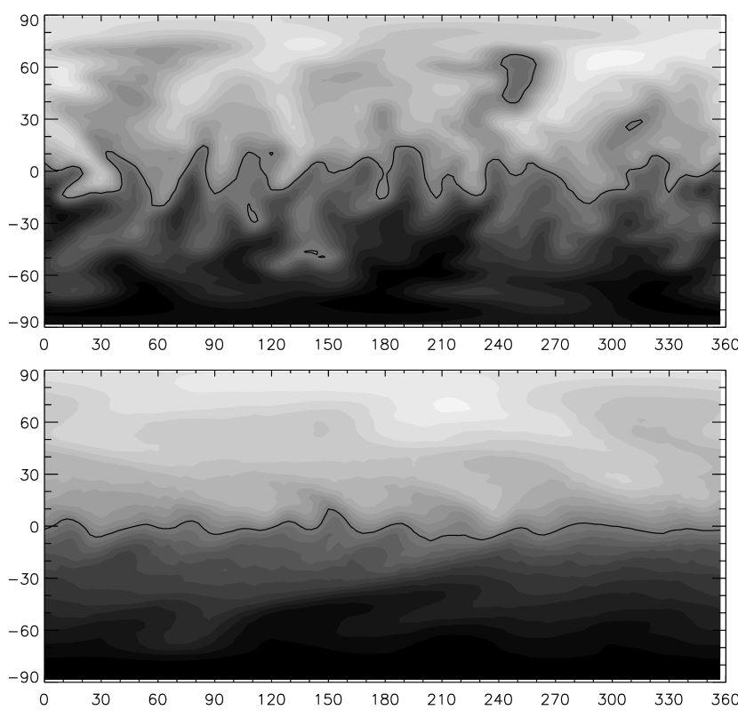
Figure 17: Maps of the radial component of the magnetic field, $B_{r}$, on the surface of the star (as fig. 4), in the aligned-rotator case, Roberts field, with $\Omega=0.5$, at two times: $t=386.9$ and $925.1$. Clearly, the amplitude of the instability away from the equator decreases as the field energy and therefore Alfvén frequency fall.

Figure 18: The fraction $|v_{r}|/\sqrt{v_{\phi}^{2}+v_{\theta}^{2}}$ (of the $m=13$ mode, integrated over the interior of the star in the $\theta,\phi$-plane) against time. It is clear that, after a short early phase, the radial (parallel to gravity) displacements are indeed much less than the horizontal (perpendicular to gravity) displacements.

Acknowledgements. The author would like to thank Henk Spruit for valuable discussions and suggestions, as well the the referee, Matthias Rheinhardt, for comments which led to significant improvements in the paper.

References

- Angel et al. (1974) Angel, J.R.P., Carswell, R., Strittmatter, P.A., Beaver, E.A. and Harms, R. 1974, ApJ, 194, L47.
- Babcock (1947) Babcock, H.W., 1947, Astrophys. J., 105, 105.
- Borra & Landstreet (1980) Borra, E.F. and Landstreet, J.D., 1980, ApJSuppl, 42, 421.
- Braithwaite (2006) Braithwaite, J., 2006, A&A, 453, 687.
- Braithwaite & Nordlund (2006) Braithwaite, J. and Nordlund, Å, 2006, A&A, 450, 1077.
- Braithwaite & Spruit (2004) Braithwaite, J. and Spruit, H.C., 2004, Nature, 431, 891.
- Braithwaite & Spruit (2006) Braithwaite, J. and Spruit, H.C., 2006, A&A, 450, 1097.
- Flowers & Ruderman (1977) Flowers, E. and Ruderman, M.A., 1977, ApJ, 215, 302.