Beyond Caustic Crossings: Properties of Binary Microlensing Light Curves

Abstract

Binary microlensing light curves have a variety of morphologies. Many are indistinguishable from point lens light curves. Of those that deviate from the point lens form, caustic crossing light curves have tended to dominate identified binary lens events. Other distinctive signatures of binary lenses include significant asymmetry, multiple peaks, and repeating events. We have quantified, using high resolution simulations, the theoretically expected relative numbers of each type of binary lens event, based on its measurable characteristics. We find that a microlensing survey with current levels of photometric uncertainty and sampling should find at least as many non-caustic crossing binary lens events as caustic crossing events; in future surveys with more sensitive photometry, the contribution of distinctive non-caustic crossing events will be even greater. To try to explain why caustic crossing light curves appear to be so dominant among the published binary lensing events, we investigate the influence of several physical effects, including blending, sampling rate, and various binary populations.

1. Introduction

1.1. Background

In gravitational microlensing, a lens and a more distant source pass near each other in the sky, causing an apparent brightening (or magnification) of the source that varies with time as the alignment changes. In the simplest case, when the source is a point source and the lens is a point mass, the light curves associated with these events are described by a simple formula (Einstein, 1936). Relative to this point lens form, the light curves produced by a binary lens, such as a binary star, are much more diverse.

General relativity is a non-linear theory, and binary lens light curves can therefore differ significantly from the sum of their two point lens components. Furthermore, although the shape of the light curve associated with any given event can be computed to arbitrary accuracy, there is no simple analytic formula for binary lens light curves. These light curves can be practically indistinguishable from point lens light curves, or they can be distinctive, as in the case of caustic crossing events, which exhibit spikes of divergent magnification. Other features not found in point lens light curves include asymmetry in time, multiple local maxima, and repeated events, which comprise two distinct brightenings separated by a return to baseline.

The distinctive events published to date by surveys such as MACHO and OGLE have tended to be dominated by caustic crossing events. The MACHO data contain 21 known binary lensing events, of which 14 were caustic crossing; toward the bulge, 12 out of 16 binary events showed caustic crossings (Alcock et al., 2000). The OGLE III 2002-2003 season produced 24 identified binary lensing events, of which 17 were caustic crossing (Jaroszynski et al., 2004), and the 2004 season produced 25 events, of which 22 were caustic crossing (Jaroszynski et al., 2006).

1.2. Smoothly perturbed events

Our main focus is on binary lensing events that differ significantly from the point lens form, but that do not exhibit caustic crossings. We call these events smoothly perturbed if they differ significantly from the best fit point lens model. The amount by which they must differ from the point lens form in order to be considered perturbed depends on the photometric uncertainty of a survey. Our main question is: for typical values of photometric uncertainty, how many such smoothly perturbed events are expected for each detected caustic crossing event? The answer to this and similar questions depends on the characteristics of the binary lens, specifically the mass ratio $q$ and the orbital separation $a$.

In §2, we introduce the binary lensing parameters, and explore the dependence of the rates of different types of light curves on these parameters. In §3 we describe the simulations we have used to calculate these relative rates numerically. In §4 we give the results for individual binary lenses over the ranges of our simulation, as characterized by a set of binary parameters. In §5 we give the results for typical populations of binary lenses and study the implications. We find that current surveys should identify significantly more smoothly perturbed binary lens event than surveys have until now.

2. Lensing geometry

2.1. Lensing formula

The magnification associated with a binary lens depends on the binary parameters and the relative locations of the source and of the lens components on the plane of the sky. As the relative positions change, we can compute the magnification at each time (Mao & Paczynski, 1991; Schneider et al., 1992; Petters et al., 2001).

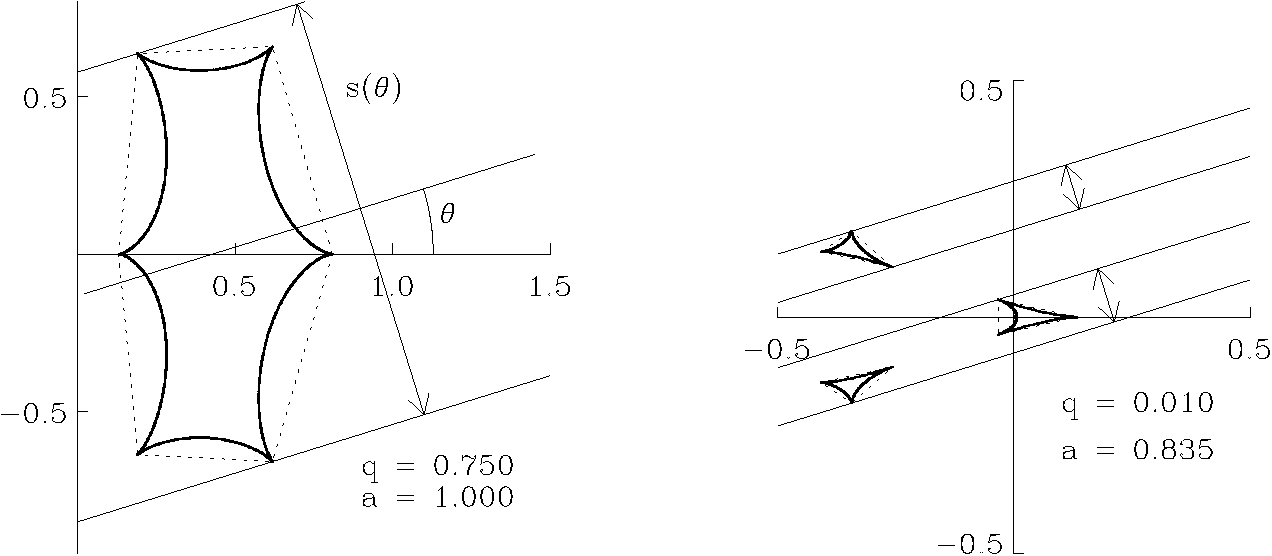
Figure 1.— Graphical depiction of $\langle s\rangle$ for caustic crossing events for two specific binaries. The left panel shows the binary $(q,a)=(0.750,1.000)$, which has a single connected caustic. The $x$-$y$ plane shown is the lens plane, with lengths measured in units of the Einstein angle $\theta_{E}$. For a given value of $\theta$, $s(\theta)$ is the width of the caustic region, as seen from that angle. The minimum bounding polygon (dashed) has a perimeter equal to $\pi$ times the average value of $s(\theta)$, that is, $\pi\langle s\rangle$. Since this polygon is defined by the positions of the cusps at the corners, we can calculate $\langle s\rangle$ from the cusp positions alone, and check the result against the simulation. The right panel shows the binary $(q,a)=(0.010,0.835)$, for which there are three disconnected caustics. In this case, $s(\theta)$ may be the sum of two or three widths. The diagram shows $s(\theta)$ for the same value of $\theta$ as the left diagram. Again it is possible to calculate $\langle s\rangle$ from the cusp positions alone.

It is convenient to express the angular positions and angular distances involved in units of the Einstein angle $\theta_{E}=\sqrt{\frac{4GM}{c^{2}}\frac{D_{S}-D_{L}}{D_{L}D_{S}}}$, where $M$ is the total mass of the lens, $D_{S}$ is the distance to the source, and $D_{L}$ is the distance to the lens. For a given $M$, the lens is described by two parameters, the mass ratio $q=M_{2}/M_{1}$ and the instantaneous angular separation $a$, which is measured in units of $\theta_{E}$. $M_{1}$ and $M_{2}$ are the mass of the primary and the secondary, and $M=M_{1}+M_{2}$.

To define the coordinate system, we place the primary at the origin and the secondary on the positive $x$-axis. A point source is completely described by its position $(x_{s},y_{s})$ in this coordinate system.

The formula for the magnification, $A(t)$, is simply a function of the binary parameters $(q,a)$ and the angular source position $(x_{s}(t),y_{s}(t))$: $A(q,a,x_{s}(t),y_{s}(t))$. We use as the units of time the Einstein angle crossing time $t_{E}=\theta_{E}/\omega$, where $\omega$ is the angular speed of the source relative to the fixed lens.

We consider only the case where the lens is static, so neither $a$ nor the binary’s orientation changes. The angular rotation of a binary lens over the course of an event is expected to be small. This is because, although binaries with a wide range of separations may act as lenses, the binary nature is only evident when the projected separation between the components is on the order of $\theta_{E},$ which is typically larger than an AU for stellar lenses. The orbital periods therefore tend to be longer than the event durations, which are on the order of weeks to months. Dominik (1998) gives more detailed criteria for when binary rotation is likely to be significant.

Thus we consider the source trajectory to be a straight line in the lens plane, defined by $b$, the angular distance of closest approach to the lens center of mass, and $\theta$, the angle the trajectory makes with the binary axis (defined to be the $x$-axis):

$$x_{s}(t) = -b\sin\theta+t\cos\theta+a_{1}$$ (1)

$$y_{s}(t) = b\cos\theta+t\sin\theta$$ (2)

Here $a_{1}=aM_{2}/M$ is the $x$-coordinate of the lens center of mass. Symmetry with respect to the binary axis, and symmetry with respect to time reversal, allow us to cover the complete parameter space by considering values of $\theta$ in the interval $(0,\pi/2)$.

2.2. The relative rate measure $\langle s\rangle$

We consider a light curve to contain an event if its maximum magnification is greater than a certain value, $A_{\rm cut}$. The rate for lensing events is given by $\sigma\,s\,\omega$, where $\sigma$ is the source density, and $s$ is the width of the lensing region, that is, the region bounded by the isomagnification contour in the lens plane corresponding to the cutoff magnification. Then for a point lens, with $A_{\rm cut}=1.34,$ the lensing region is a circle of radius $\theta_{E}$, and so $s=2\theta_{E}$. For a given binary lens, the lensing region is not circular, so $s$ depends on the angle of approach $\theta$. $s(\theta)$ is the linear size of the lensing region as seen from the angle $\theta$. The average value of $s(\theta)$, $\langle s\rangle,$ for a given binary represents the lensing region’s average angular width. If a large number of sources were to pass behind this binary, the event rate would be $\sigma\,{\langle s\rangle}\,\omega$. Since the only dependence on the intrinsic properties of the lens is through the factor ${\langle s\rangle}$, it is this quantity we will compute for different lenses. Taking $\sigma$ and $\omega$ to be the same for all potential lenses, the ratio of rates does not depend on them. We can therefore use the ratios of the values of $\langle s\rangle$ to compare relative average rates for the total numbers of events generated by different lenses.

For a given binary lens, different source paths produce light curves with different characteristics. For example, paths that cross the caustics produce light curves with distinctive wall-like structures, the so-called caustic crossing light curves. The rate of such events is determined by the dimensions (in angular units in the lens plane) of the caustics (see Figure 1). The value $s_{cc}(\theta)$ measures the extent of the caustics perpendicular to the direction of approach specified by $\theta$.

$\begin{array}[]{cc}\includegraphics[width=216.81pt]{nex.png}&\includegraphics[width=216.81pt]{asym.png}\end{array}$

Figure 2.— Peak count and asymmetry parameter in the light curve corresponding to a given $b$ and $\theta$, with $(q,a)=(1.0,1.0)$ held fixed. The graph is not shown in $x$-$y$ coordinates like in Figure 1; $b$ and $\theta$ are similar to the polar coordinates in that plane. The left panel shows the number of peaks color coded. Colors gray, red, yellow, orange, green, and blue correspond to 1, 2, 3, 4, 5, and 6 peaks, respectively. The right panel shows the asymmetry parameter $k$ (see §3.3.2), color coded logarithmically, with black the most symmetric ($k\approx 0$) and white the least symmetric ($k\approx 1$). In both panels, black sinusoidal curves show the $b$-value of the caustic cusps as a function of $\theta$; any trajectory with values of $b$ and $\theta$ between these black curves will produce a caustic crossing light curve. The black curves are easy to describe in terms of the cusp locations in the $x$-$y$ plane (see Figure 1), and so $\langle s\rangle$ for caustic crossings may be computed from them. For other light curve characteristics, however, $\langle s\rangle$ is more complicated. For instance, $\langle s\rangle$ for single-peaked events is given by $\frac{1}{\pi}$ times the area of the gray region in the left panel. That is, $\langle s\rangle=\frac{1}{\pi}\int_{0}^{\pi}\int_{-\infty}^{+\infty}N(b,\theta)\,db\,d\theta$, where $N(b,\theta)$ is 1 at any point in the gray region and 0 elsewhere. In the right panel, $\langle s\rangle$ for light curves with a certain amount of asymmetry corresponds to the size of a contour for a certain brightness. Any other $\langle s\rangle$ is similarly defined in terms of a region on the $b-\theta$ graph.

Even event types that do not correspond to crossing an easily defined region, such as smoothly perturbed events, may be thought of as having an effective width, which $s(\theta)$ measures. For a given $q$, $a$, and $\theta$, there is a range of values of $b$ that correspond to light curves with any property we choose to investigate, such as being smoothly perturbed. This range may be connected or disconnected, but generally, the bigger the size of the range (or the sum of the sizes of the parts), the more likely that a randomly chosen $b$ will correspond to a light curve with the given property. The size of this range, then, is $s(\theta)$. (In set-theoretic terms, $s(\theta)$ is the 1-D Lebesgue measure of the set of all values of $b$ that correspond to the property in question, for fixed $q$, $a$, and $\theta$.)

We can therefore compute $s(\theta)$ for any given property by generating many different source paths with incidence angle $\theta,$ and counting the fraction of all events in which the light curve exhibits that property. Specifically, we generate light curves for many values of $b$ for each value of $\theta$. For each such trajectory, we sample the magnification at a sequence of times $t_{i}$, compute the corresponding $A_{i}=A(t_{i})$, and examine the resulting light curve. The sampling rate $\Delta t$ is the difference between consecutive values of $t$. As a default we choose $0.01\theta_{E}$, but in §4.3 we explore how the results vary for different sampling rates.

Once we have determined $s(\theta)$, the next step is to average over the possible values of $\theta$: $\langle s\rangle=\frac{1}{2\pi}\int_{0}^{2\pi}s(\theta)\,d\theta$. For some event types, there is a simple expression for $s(\theta)$, so we may compute $\langle s\rangle$ analytically. Generally, however, no such simple expression exists, so we must perform the integration numerically with simulations.

From the values of $\langle s\rangle$ for various properties, we may compute the relative rates for light curves with those properties. For instance, suppose that for a fixed $q$ and $a$, the value for caustic crossing events is $\langle s_{cc}\rangle$, and the value for all events (i.e. light curves that exceed our minimum cutoff magnification $A_{\rm cut}$) is $\langle s_{e}\rangle$. Then, for this binary alone, the probability of an event being a caustic crossing event is $\langle s_{cc}\rangle/\langle s_{e}\rangle$, and this also eqquals the relative rates for caustic crossing events to all binary events. Realistically, however, there is a population of binary lenses described by a probability distribution function $P(q,a)$. In that case, the relative rate we seek is given by $\int\langle s_{cc}(q,a)\rangle P(q,a)\,dq\,da/\int\langle s_{e}(q,a)\rangle P(q,a)\,dq\,da$. Our results for individual binaries are given in §4.1, and our results for populations of binaries are given in §4.2.

2.3. Caustic crossing $\langle s\rangle$

For caustic crossing light curves, there is a simple analytic expression for $s(\theta)$ and thus for $\langle s\rangle$. This is because caustic crossing light curves are defined by whether the trajectory crosses the caustic region. We may therefore determine whether a trajectory corresponds to a caustic crossing light curve without generating the light curve itself. So for caustic crossings, $s(\theta)$ is the width of the caustic region as seen from the angle $\theta$ (see Figure 1), and $\langle s\rangle$ is the average width of this region.

It can be shown that the average width of any convex region (and thus $\langle s\rangle$ for any property that corresponds to crossing the region) is equal to $\frac{1}{\pi}$ times the region’s perimeter. For example, not surprisingly, for a circular region, $\langle s\rangle$ is $\frac{1}{\pi}$ times the circle’s circumference, that is, its diameter. For a concave region like a caustic region, we only need to draw the smallest convex shape that encloses the region, and then, since every trajectory that crosses this region will cross this convex shape and vice versa, $\langle s\rangle$ is equal to $\frac{1}{\pi}$ times the perimeter of this enclosing shape.

Caustics are everywhere concave except at a small nuber of points called cusps, so the bounding shape is a polygon (as shown in Figure 1), and $\langle s\rangle$ can be computed directly from the locations of the cusps. Specifically, it is:

$$s(\theta)=\frac{1}{\pi}\sum_{p=0}^{n-1}\sqrt{(x_{p+1}-x_{p})^{2}+(y_{p+1}-y_{p})^{2}}$$ (3)

Here the $(x_{p},y_{p})$ are the locations of the cusps that are vertices of the bounding polygon and $n$ is their count; for a single caustic region $n$ will be either 5 or 6 (and for simplicity of notation, let $(x_{n},y_{n})=(x_{0},y_{0})$). The cusp locations are given by the simultaneous roots of two polynomials of degree 11 and 10 (see Schneider et al. (1992) Eq. 6.23). These roots can be computed to sufficient precision with minimal difficulty in a program such as Mathematica.

For a binary lens, there are either one, two, or three separate caustics. The above analysis strictly applies only to binaries with a single caustic, but it can easily be made to apply to the other cases as well. For binaries with two caustics, we need only to compute $\langle s\rangle$ for trajectories that cross one or the other or both: if $s_{1}(\theta)$ corresponds to crossing the first caustic region, $s_{2}(\theta)$ corresponds to crossing the second, and $s_{12}(\theta)$ corresponds to crossing both, then corresponding to the overall feature of crossing one or the other or both is $s(\theta)=s_{1}(\theta)+s_{2}(\theta)-s_{12}(\theta)$ (because $s(\theta)$ is the measure of the intersection of the sets for which $s_{1}(\theta)$ and $s_{2}(\theta)$ are measures). Thus for caustic crossing events, $\langle s\rangle=\langle s_{1}\rangle+\langle s_{2}\rangle-\langle s_{12}\rangle$. The value $\langle s_{12}\rangle$ can also be expressed in terms of the concave bounding shapes of the two regions, so it may be computed analytically as well. A similar formula holds for binaries with three caustics.

Thus we can easily compute $\langle s\rangle$ for caustic crossing light curves to a high precision for all $q$ and $a$. While this does lend some degree of insight, we use it primarily to check the simulations that compute it and other values numerically.

2.4. The value of $\langle s\rangle$ for other light curve features

There are other type of events that lend themselves to analysis almost as simple as the analysis for caustic crossings. For instance, if we say a light curve contains an event when its maximum magnification is greater than a threshold value $A_{\rm cut}$, then $\langle s\rangle$ for events is $\frac{1}{\pi}$ times the perimeter of the smallest convex shape that bounds the isomagnification contour for $A_{\rm cut}$. For wide binaries, repeating events (those which dip below $A_{\rm cut}$ and back up) are another example (Di Stefano & Mao 1995). When the isomagnification contour for $A_{\rm cut}$ comprises two separate convex curves, as is the case with well separated binaries, $\langle s\rangle$ for repeating events can be determined as was done for disconnected caustics above, simply from the coordinates of the points in the isomagnification contour corresponding to $A_{\rm cut}$. For multipeaked events (those with two or more local maxima), even though there is not a simple expression for $\langle s\rangle$ in terms of the perimeter of a region, a sense of whether a given trajectory will generate a multipeaked light curve can be obtained by examining how it crosses the isomagnification contours.

In general, however, there is no easier way to compute $\langle s\rangle$ than numerically. For example, Figure 2 shows that $s(\theta)$ for multipeaked events and asymmetric events are more complicated than for caustic crossing events.

3. Simulation Specifications

Our simulation generates a set of light curves for a given $q$ and $a$ by selecting values of $b$ and $\theta$, one at a time. The light curve is defined by a discrete set of times $t_{i}$ and the corresponding amplifications $A_{i}=A(t_{i})$. If the light curve contains an event (${\rm max}(A_{i})>A_{\rm cut}$), certain light curve parameters are measured. Our default value of $A_{\rm cut}$ is 1.1, that is, a 10% magnification above baseline. (For comparison with such surveys as OGLE, $A_{\rm cut}=1.34$ may be more appropriate; see §4.3.) Among light curves with events, running totals of all light curves with certain parameter values and characteristics are kept.

3.1. Trajectory selection

We wish to select values of $b$ and $\theta$ in such a way as to mimic the way they are randomly “selected” in nature. This is done simply enough by realizing that the probability distribution function for the trajectories is uniform in both $b$ and $\theta$. We select 1600 equally spaced values for $\theta$ between 0 and $\pi/2$, and for each of these determine the set of values for $b$ that will completely cover the set of events. This set is all trajectories that cross the isomagnification contours of $A(x_{s},y_{s})=A_{\rm cut}$ in the lens plane, as shown in Figure 3.

Figure 3.— Coverage of sampling. The $x$-$y$ plane shown is the lens plane, measured in units of $\theta_{E}$, as in Figure 1. For $(q,a,\theta)=(0.562,4.217,0.400)$ (chosen as a typical example), each dashed line is a trajectory for a light curve that was generated, each with a different value of $b$. Solid lines correspond to the parts of the trajectory that were identified as events. Isomagnification contours corresponding to $A_{\rm cut}=1.1$ and locations of the caustics are also shown. The sampling in $b$ used in the simulations is 50-100 times denser than that shown in this figure.

Although it is essential to completely cover these isomagnification contours, it is desirable to limit the number of light curves generated that do not cross the contours. Starting with a given binary, defined by the values $(q,a)$, and considering an individual value of $\theta,$ there is a limited range of values of $b$ that yield events. For a given $\theta,$ we first identify a value of $b$ for which we know there is an event. We accomplish this by starting with the fact that, for any value of $A_{\rm cut},$ there are isomagnification contours that enclose caustics, as in Figure 3 with two separate contours, each containing one caustic. We therefore begin sampling $b$ by choosing a value that hits a caustic cusp. We then continue by choosing a sequence of values of $b$, separated by $\Delta b$, from the original one. We sample in both perpendicular directions (“up” and “down”) from the original trajectory, keeping $\theta$ fixed. Therefore, by starting at each caustic and moving in both directions by an amount $\Delta b$ (equal to 0.002 for most binaries in the simulation) for as long as events are generated, we can be sure to cover the entire contour, while limiting non-event light curves. (This corresponds to stopping when the white area is reached in the left panel of Figure 2.) The caustics, as mentioned in the previous section, are bounded by their cusps, which can be located to high precision before the simulation is run. Double sampling is avoided by maintaining a running list of the range of $b$ sampled so far.

For each event, as the source gets far enough away from the lens, the magnification drops toward 1, so for any trajectory there is a certain range of $t$ for which $A(t)>A_{\rm cut}$. The limits of $t$ should be chosen to at least cover this range, but because the tails with $A(t)<A_{\rm cut}$ are ignored, it is a good idea to reduce these limits as much as possible while still ensuring that all regions above $A_{\rm cut}$ are covered. Therefore, as with $b$, we chose to stop light curve generation when $A(t)<A_{\rm cut}$ and all the caustics have been passed (notice the rectangular shape of the dashed lines in Figure 3). Starting from $t=0$ and moving in both directions, this allows us to avoid computing many unneeded magnification values.

3.2. The magnification function

The time consuming part of light curve generation is determining the value of the magnitude function $A(q,a,x_{s},y_{s})$. To compute it, one determines the locations in the lens plane of the lensing images, from which $A$ can be computed analytically. The positions $(x_{i},y_{i})$ of the images, however, cannot be computed analytically. They are expressed in terms of the simulataneous roots of two polynomials in $x_{i}$ and $y_{i}$ of degree 5 and 4, or alternately in terms of a single complex polynomial of degree 5 (Erdl & Schneider, 1993).

The method we choose to determine these roots numerically is Newton’s Method with polynomial deflation (Press et al., 1992) on the real fifth-degree polynomial given in (Asada et al., 2004). Because it uses real (rather than complex) arithmetic, this method, combined with some other minor optimizations, allows for a great improvement in speed over root finding for the complex polynomial.

Finally, after up to several hundred calls to the function, the light curve is complete, and stored as an array of $t_{i}$ and $A_{i}$ values. We may then analyze it, and record its characteristics and statistical parameters.

3.3. Defined parameters

We seek to quantify the amount by which a binary lens light curve differs from a point lens light curve. To this end we define three parameters. For a point lens light curve, the value of each parameter is exactly zero, and light curves with more pronounced deviations from the point lens form have higher parameter values. Our three parameters relate to the least-squares fit of a point lens, the asymmetry of the curve, and whether the light curve exhibits more than one local maximum, i.e., whether it is multi-peaked.

3.3.1 Best fit $\sigma_{P}$

The most straightforward way to evaluate whether a light curve is consistent with a certain model is to fit it to that model using a least-squares fit. Therefore we begin by fitting each binary lens light curve with a standard 3-parameter point lens form, known as the Paczyński model. (We assume that in observations, the baseline can be determined arbitrarily well, so it is not considered a fit parameter.) As usual, we define the closest point lens model, $A_{\rm PL}(t)$, to be the one which minimizes the sum of the squared differences between the values of the simulated binary lens light curve, $A_{i},$ and the model.

$$\sum_{i=1}^{n}\Big{(}A_{i}-A_{\rm PL}(t_{i})\Big{)}^{2}$$ (4)

The binary lens light curve offers a certain amount of intrinsic deviation from the point lens model, characterized by this sum-of-squares quantity. In real observations, there will be additional deviation due to the photometric uncertainty. Roughly speaking, when the intrinsic deviation is larger than the photometric deviation, the binary nature of the light curve will be evident through least-squares fitting. When the intrinsic deviation is smaller, $A_{\rm PL}$ will provide an acceptable fit to the binary lens light curve.

Thus we define our first parameter, $\sigma_{P}$, as a measure of how large the photometric uncertainty would need to be in order for the observed light curve to be well fit by a point lens model. This parameter is given by the root-mean-squared difference between the simulation light curve and the best fit light curve:

$$\sigma_{P}=\Big{[}\frac{1}{n-3}\sum_{i=1}^{n}\Big{(}A_{i}-A_{\rm PL}(t_{i})\Big{)}^{2}\Big{]}^{1/2}$$ (5)

Note that $\sigma_{P}$ does not actually quantify the goodness of fit of a point lens model to a simulated binary lens light curve; since there are no uncertainties associated with the simulated light curve, such a statistic is meaningless. For an observed light curve with associated uncertainties, the goodness of fit is quantified by the reduced $\chi^{2}$ test statistic. Its formula is very similar to our formula for $\sigma_{P}$:

$$\chi^{2}=\frac{1}{n-3}\sum_{i=1}^{n}\frac{\big{(}A_{i}-A_{\rm PL}(t_{i})\big{)}^{2}}{\sigma_{i}^{2}}$$ (6)

The $t_{i}$, $A_{i}$, and $\sigma_{i}$ are the times, magnifications, and uncertainties of the observed light curve, of which there are $n$. $A_{\rm PL}(t)$ is the three parameter point lens fit chosen such that $\chi^{2}$ is minimized. For our purposes, we will assume that the uncertainties $\sigma_{i}$ are equal in magnitude space to a general survey parameter $\sigma_{phot}$ that quantifies the photometric uncertainty of the survey.

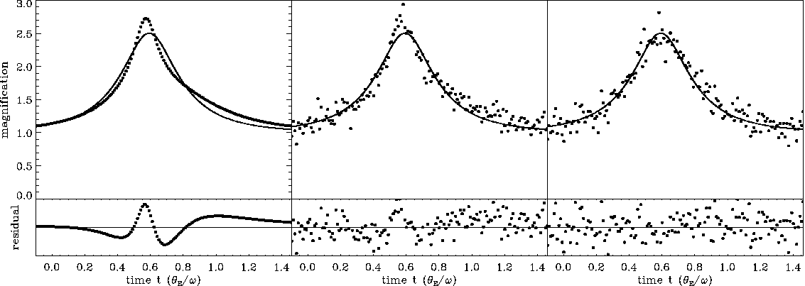
Figure 4.— Comparison of residuals for an asymmetric binary lens light curve and a point lens light curve. The binary lens light curve in the left panel (dots, corresponding to simulated observations) has a best fit point lens light curve as shown by the solid curve. It has a best fit parameter of $\sigma_{P}=0.09$, the root-mean-square deviation from this fit, but an asymmetry parameter of $k=0.21$. The center panel shows the same observations with $10\%$ Gaussian error added; if this light curve were fit assuming $10\%$ photometric uncertainty, the best fit test statistic would be $\chi^{2}<2$. The right panel shows the same best fit point lens, with enough Gaussian error added to give it a comparable $\chi^{2}$. Below each light curve are shown the residuals after subtracting out the best fit curve. Although the average size of the residuals is comparable in the two right panels, the residuals of the center panel show much more apparent structure, as expected.

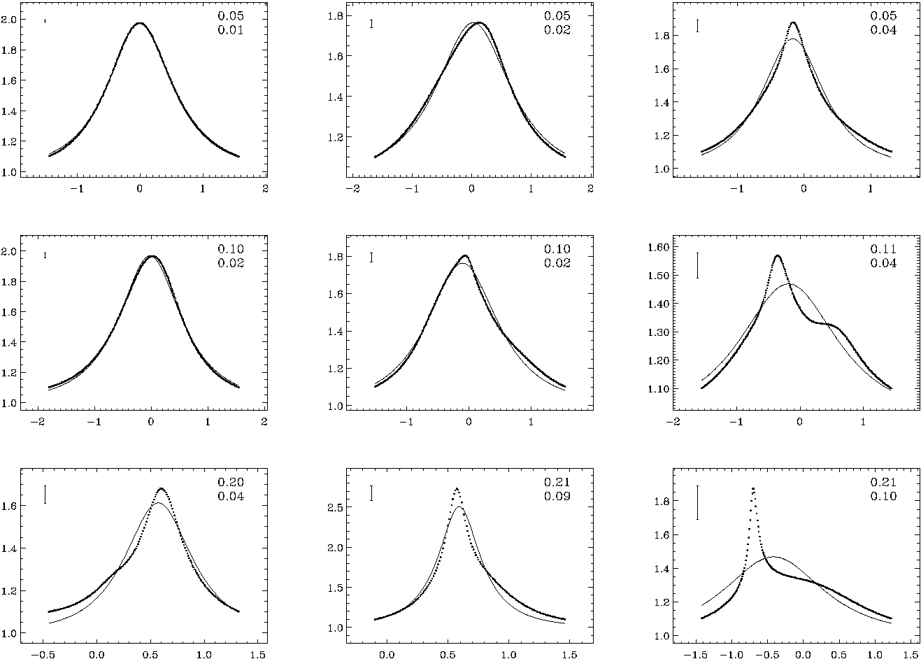
Figure 5.— A variety of binary lens light curves along with their best fit point lens models. In the upper right of each panel is shown the asymmetry parameter $k$ followed by the best fit parameter $\sigma_{P}$. The top, middle, and bottom rows show light curves with asymmetry parameter $k$ equal to approximately 5%, 10%, and 20%. The error bar in the upper left has a value of $2\sigma_{P}$; thus it is the size of the error bar necessary to make the best fit $\chi^{2}$ equal unity. Generally speaking, the greater the parameter values, the further the light curves are from their point lens models.

Thus, roughly speaking, for a given binary lens light curve, $\sigma_{P}$ is the critical value for the photometric uncertainty: if $\sigma_{phot}>\sigma_{P}$, the light curve will be well fit by a point lens model, and if $\sigma_{phot}<\sigma_{P}$, it will not. Strictly speaking, if a binary lens light curve with intrinsic deviation $\sigma_{P}$ is observed with uniform, uncorrelated, Gaussian random photometric errors with standard deviation $\sigma_{phot}$, and then fit with a point lens model, the reduced $\chi^{2}$ statistic will have an expected value (for $n\gg 1$) of $\chi^{2}=1+(\sigma_{P}/\sigma_{phot})^{2}$. Therefore, for $\sigma_{P}>\sigma_{phot}$, the expected value of $\chi^{2}$ exceeds 2, so the point lens model would probably be identified as a bad fit. This is the basis of our rule of thumb that a survey with an average photometric uncertainty of $\sigma_{phot}$ should discriminate as non-point lens a binary lens light curve with $\sigma_{P}>\sigma_{phot}$.

3.3.2 Asymmetry parameter $k$

Model fitting reveals how much a binary lensing light curve differs from the point lens model, but not in what way. Because point lens light curves are always symmetric in time, i.e., $A(t)$ is an even function, one obvious way in which we expect some binary lens light curves to differ is by exhibiting some asymmetry with respect to time reversal. Therefore we define an asymmetry parameter $k$ that is 0 for a symmetric light curve, and larger for more asymmetric ones. The parameter $k$ is based on the Chebyshev coefficients $T_{n}$, which are the convolution of the light curve function $A(t)$ with Chebyshev polynomials, as in Di Stefano & Perna (1997). For even $n$ the polynomial is an even function, and for odd $n$ the polynomial is an odd function. Therefore a function with even symmetry has $T_{n}=0$ for all odd $n$, and a function with some asymmetry must have $T_{n}$ significantly nonzero for some odd $n$. We then define the asymmetry parameter to be the ratio of the root-mean-square average of the odd coefficients to the even coefficients:

$$k=\Big{(}{\displaystyle\sum_{n=1}^{\infty}T_{2n+1}^{2}}\Big{/}{\displaystyle\sum_{n=1}^{\infty}T_{2n}^{2}}\Big{)}^{1/2}$$ (7)

One use of the asymmetry parameter is to characterize the way in which a particular light curve deviates from the point lens form. We note, however, that when we apply model fits to light curves with pronounced asymmetries, the residuals to the best point lens fit are not randomly distributed in time, but instead exhibit some structure. That is, the deviations from the point lens light curve are correlated, even when $\sigma_{P}$ is small. Thus the parameter $k$ can identify light curves with small but correlated residuals, whereas the parameter $\sigma_{P}$ cannot. An example of two light curves with identical $\chi^{2}$ but different $k$ is shown in Figure 4.

In this paper we identify light curves that are smoothly perturbed from a point lens form by their values of $\sigma_{P}.$ We note, however, that in future work it may be possible to use the asymmetry parameter to identify binary lens light curves, even if the best fit parameter fails to distinguish them from point lens events. Figure 5 shows typical light curves with various intermediate values of $\sigma_{P}$ and $k$. Extremely point lens-like or extremely perturbed events will easily stand out with any choice of statistics.

3.3.3 Multipeak parameter $p$

This parameter is identically 0 for any light curve with a single peak. For light curves with two peaks, it is the difference between the first peak and the intervening minimum, or the difference between the second peak and the intervening minimum, whichever is smaller. The idea is that if differences of less than $p$ were undetectable, the multipeaked nature of the light curve would go unnoticed. For light curves with three or more peaks, it is the largest such value for any of the minima in the light curve:

$$p={\rm Max}_{i}({\rm Min}(A_{{\rm max},i},A_{{\rm max},i+1})-A_{{\rm min},i})$$ (8)

where $A_{{\rm min},i}$ is the magnitude at the $i$th minimum and $A_{{\rm max},i}$ is the magnitude at the $i$th maximum.

4. Results

4.1. Results for individual binaries

Figure 6.— The relative rate measure $\langle s\rangle$ for various types of binary lensing events for certain fixed values of $q$. For each of the four values of $q$ as indicated in the left panels, $\langle s\rangle$ is plotted against $a$. The types of events identified are: caustic crossing events (orange dotted curve), smoothly perturbed events ($\sigma_{P}>0.1$, blue solid curve), point lens like events ($\sigma_{P}<0.1$, red dashed curve), and the total of these three categories (black solid curve). Note particularly that there are many values of $q$ and $a$ where the smoothly perturbed events outnumber the caustic crossing events. The right panels show the same data as the left panels, except on a logarithmic plot. The right panels also show the relative rates for two more types of events, repeating events ($A_{\rm min}<A_{\rm cut}$, solid yellow curve) and asymmetric events ($k>0.1$, dashed green curve). There is some overlap between these two categories, and between these categories and the others.

$\begin{array}[]{cc}\includegraphics[width=216.81pt]{contour-all.png}&\includegraphics[width=216.81pt]{contour-pll.png}\\ \includegraphics[width=216.81pt]{contour-unfit.png}&\includegraphics[width=216.81pt]{contour-cross.png}\\ \includegraphics[width=216.81pt]{contour-asymm.png}&\includegraphics[width=216.81pt]{contour-repeat.png}\end{array}$

Figure 7.— Contour plots of $\langle s\rangle$ vs. $q$ and $a$ for the entire range covered by our simulations. Each panel corresponds to a different type of event: all events ($A_{\rm max}>A_{\rm cut}$), point lens like events ($\sigma_{P}<10\%$), smoothly perturbed events ($\sigma_{P}>0.1$), multi-peaked events at 10% (multipeak $k>0.1$), and finally repeating events ($A_{\rm min}<A_{\rm cut}$). Consecutive contours are separated by 0.1 with dark contours every 0.5. Overwritten numbers show the same data in tabular form. Notice that generally there are more variations with varying $a$ than with varying $q$, and that the curves exhibiting binary signatures exist most in the “critical zone” around $a=1$. For a point lens light curve, $\langle s\rangle$ for the total number of curves would be 3.35.

Figures 6 and 7 depict the relative event rates $\langle s\rangle$ as a function of $q$ and $a$. Figure 6 plots these rates for several fixed values of $q$, and Figure 7 shows contour plots for the entire range of $q$ and $a$ covered by our simulation. The graphs in Figure 6 are vertical cross sections of the contour plots in Figure 7.

The total rate of events (light curves for which $A_{\rm max}>A_{\rm cut}$) is shown as the top, solid black curve (“all”) in each panel of Figure 6, and in the top left panel of Figure 7. The values we have computed can be checked analytically both for low values of $a,$ where the lens essentially acts as a single point lens, and for high values of $a,$ where the lens acts approximately as two independent point lenses. In the limit of small $a,$ the event rate is determined simply by our cutoff magnitude. For $A_{\rm cut}=1.34$, corresponding to $b\leq\theta_{E}$ (or $b\leq 1$ in our units) for a point lens, the rate would be $\langle s\rangle=2$. For our default value of $A_{\rm cut}=1.1$, this rate is $\langle s\rangle=3.35$. On the other hand, for $a$ very large, the masses act as two separate point lenses, each with its own Einstein radius proportional to the square root of its mass. Thus the event rate increases by a factor of $\frac{1+\sqrt{q}}{\sqrt{1+q}}$. This factor is maximized with a value of $1.414$ for $q=1$, producing an overall event rate of $\langle s\rangle=4.73$. This is the value approached, for large $a$, by the solid black curves in Figure 6.

The increase in event rate for large $a$ causes an interesting effect. Although the lensing optical depth depends only on the total mass of the lens and not on $a$, the event rate increases from the point lens value as $a$ increases. Thus a lens population consisting of equal total masses of binaries and single stars would produce more binary lens than single lens events, even though binaries and point lenses would contribute the same amount to the lensing optical depth. Note that most of the binary events would be indistinguishable from point lens events.

Also plotted are rates for the two main types of binary perturbations: non-caustic crossing but with $\sigma_{P}\geq 10\%$ (smoothly perturbed events), and caustic crossing. These are shown in Figure 6 with a dotted orange curve and a solid blue curve, respectively, and in the middle two panels of Figure 7. All events that are not perturbed in either of these two ways are shown as “point lens like” events, with a red dashed curve in Figure 6, and in the upper right panel of Figure 7. The rate for “all” events, that is, the total rate, is the sum of the rates for smoothly perturbed, caustic crossing, and point lens like events.

For all values of $q$, there are values of $a$ for which the smoothly perturbed events outnumber the caustic crossing events. In Figure 6, this is where the blue solid curve is above the orange dotted curve. In Figure 7, this can be seen by comparing the overlaid numbers at the top and bottom of the middle two panels. An increase or decrease in $a$ from $a=1$ results in the smoothly perturbed event rate exceeding the caustic crossing rate. The fact that it occurs on both sides of $a=1$ suggests that a binary distribution function weighted toward either high or low $a$ will not tend to favor caustic crossing events over smoothly perturbed events.

Binary perturbations are most frequent close to $a=1$ for all values of $q$, and there tends to be more variation of event rates over the range of $a$ covered by our simulation than over the range of $q$. This can be seen by the largely horizontal contours in Figure 7.

Small $q$ corresponds to a low mass secondary, approaching the planet in the limit $q\ll 1$. For the most part, for small $q$, both event characteristics and event rates approach those of point lenses. Nevertheless, there are two regions of parameter space where planetary systems can provide distinctive lensing signatures. The first is for values of $a$ close to unity. In this “resonant” regime (Mao & Paczynski, 1991; Gould & Loeb, 1992), the most obvious evidence of the existence of the planet is provided by caustic crossings, which punctuate an otherwise point lens like light curve. The second is for larger values of $a$, where asymmetry in otherwise point lens like events, and also repeating events provide evidence of the low mass companion (Di Stefano & Mao, 1996; Di Stefano & Scalzo, 1999a, b). In this paper we focus on the regime of binary stars. As $q$ increases from near $0$, binary signatures become more frequent and more pronounced, with relatively little effect for varying $q$ greater than $\sim 0.2$ (see Figure 7). Because values of $q$ near or larger than $0.2$ are favored by binary distributions, e.g., the distribution studied by Duquennoy & Mayor (1991), we expect the distribution in $a$ to have a more pronounced effects than the choice of realistic distribution in $q$.

Although the strongest binary signatures occur within an order of magnitude of $a=1$, there is a dip in binary signatures in the center of this range, very near to $a=1$. This can be seen in Figure 6 as a dip in total event rate and a smaller dip in caustic crossing event rate. This can be explained in terms of the geometric considerations of the lens plane from §2. When $a$ is very close to 1, the caustics (and thus the region of binary perturbations) are roughly equal in size in both dimensions. As $a$ increases or decreases, the caustics stretch in one dimension or the other, and so they have a larger extent in the lens plane. The caustic crossing event rate peaks just as the caustics transition from connected to disconnected, and the perturbed event count peaks farther from $a=1$, with the value of $a$ at the peak determined by the value of $A_{\rm cut}$.

Although our coverage in $a$ is not infinite, spanning two orders of magnitude from $a=0.1\theta_{E}$ to $a=10\theta_{E}$, it includes the range with significant binary signatures. For any value of $q$, all binary effects will go to 0 as $a$ becomes very large or very small. In Figure 6, this is seen in all panels, as all curves but the top two go to 0 in both directions. In Figure 7, this is seen in the lower four panels, as all tabulated values go to 0 at the top and bottom of the panel.

Repeating events (multipeaked events with $A_{\rm min}<A_{\rm cut}$), and asymmetric events ($k>0.10$) are shown in the right hand (log plot) panels of Figure 6, as gold solid curves and dashed green curves, respectively. Repeating events are one type of binary behavior that does not fall off with the size of the caustics for large $a$. Rather, two separated point lenses can still produce a significant number of repeating events. This can be computed analytically as in §2. If $R$ is the rate for a point lens of the same mass ($R=3.35$ for $A_{\rm cut}=1.1$), then to leading order in $R/a$, the rate for repeating events is approximately $\frac{1}{2\pi}{\rm sech}(\frac{1}{2}\ln(q))\frac{R^{2}}{a}$. This expression goes as $a^{-1}$ whereas the caustic crossing event rate goes as $a^{-2}$.

Although asymmetric and repeating events are significantly less frequent than caustic crossing events and smoothly perturbed events, they are expected to constitute a few percent of binary lens events. We should therefore find them in any large sample of binary lensing events.

4.2. Results for populations of binaries

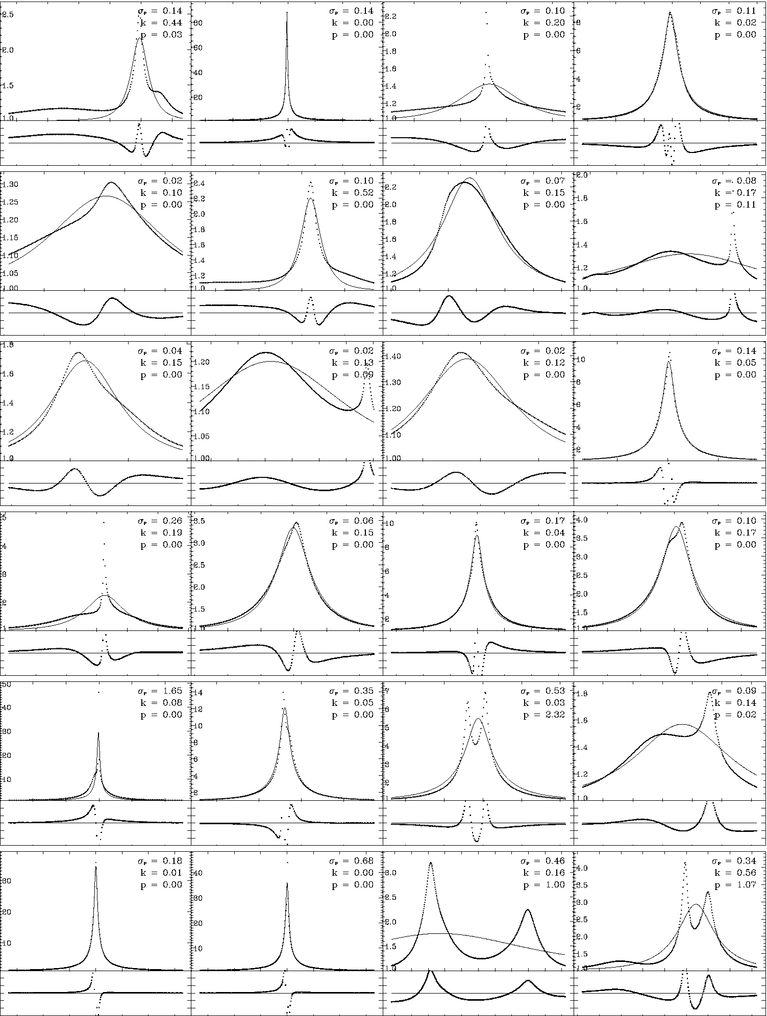
Figure 8.— Random sampling of non-caustic crossing, nonrepeating light curves perturbed at the 10% level. Each light curve is shown with its best fit point lens model. Residual plots below show the patterns of the differences between the light curve and the model. The three light curve parameters are shown in the upper right of each panel; these light curves were selected from the population that has at least one of these three parameters greater than 0.1. Horizontal (time) axis tick marks for each light curve are in units of 0.5 times the Einstein angle crossing time $\theta_{E}/\omega$. Vertical axis tick marks in the residual plots are in units of $\sigma_{P}$, and the axis ranges from $-3\sigma_{P}$ to $+3\sigma_{P}$. Our simultions show that typically, for every 13 caustic crossing events, there are 15 events that are smoothly perturbed with $\sigma_{P}>10\%$, and a total of 24 events for which at least one of the three parameters exceeds 0.10.

In order to use these results to make predictions for surveys, we must consider a population of binary lenses whose properties (mass ratios and projected orbital separations) are drawn from a realistic distribution given by a probability distribution function $P(q,a)$. Then, for instance, the overall relative rate for a given type of event is:

$$\langle s_{x}\rangle=\int\!\!\int P(q,a)\langle s_{x}(q,a)\rangle\,dq\,da$$ (9)

Note that previously we have used $\langle s\rangle$ to denote an average only over $b$ and $\theta$, but here and in subsequent sections, we use it to denote an average over all four binary parameters. As a default, we assume a distribution uniform in $q$ and log-uniform in $a$, but in §4.3 we explore how the results vary for different distributions.

For every caustic crossing light curve, there are a certain number of smoothly perturbed light curves, as shown in Figure 8. We want to find this ratio. Our default definition for smoothly perturbed events is $\sigma_{P}\geq 0.10$, but we vary this cutoff parameter value over a wide range, from 0.01 to 1.0, and show the ratio for all cutoff values.

Figure 9.— Curve showing the expected rate ratio of smoothly perturbed to caustic crossing events. The $y$-axis shows the rate $\langle s\rangle$ of events with $\sigma_{P}$ greater than the corresponding $x$-axis value, normalized to $\langle s\rangle$ for caustic crossing events. The horizontal solid line shows $\langle s\rangle$ for caustic crossing events. The horizontal solid line corresponds to equal rates of smoothly perturbed and caustic crossing events. Under our default assumptions, a survey with perfect detection efficiency of events perturbed at the $\sigma_{P}=15\%$ level would expect to find as many smoothly perturbed events as caustic crossing events. Shown as dashed horizontal lines are the ratios reported for MACHO (5.7 year data; Alcock et al. (2000); 4 perturbed events out of 16 binaries), OGLE III 2002-2003 season (Jaroszynski et al. (2004); 7 perturbed candidates out of 24 binary candidates), and OGLE III 2004 season (Jaroszynski et al. (2006); 3 perturbed events out of 25 binary candidates). Implicit in this graph are the default assumptions for our simulation, which are the selection criterion $A_{\rm cut}=1.10$, the sampling rate $\Delta t=0.01\theta_{E}$, the distribution function $P(q,a)$ uniform in $q$ and $\log(a)$, and the assumption of no blending. The following figures show how this graph is affected when these are changed.

Figure 9 shows the major results. For various cutoff $\sigma_{P}$ values, it shows the ratio of smoothly perturbed to caustic crossing events. For a cutoff value of $\sigma_{P}$ of 0.10, this ratio is slightly greater than unity. Roughly speaking, this means that a survey with $10\%$ photometry should detect more smoothly perturbed events than caustic crossing events. Naturally, the better the photometry, the larger this ratio should be. For $1\%$ photometry, the theoretical ratio is as high as 3. We can also answer the question: for what precision of photometry would the observed ratios ($4/12$ for MACHO, $7/17$ for OGLE in 2002-2003, and $3/25$ for OGLE in 2004) match the expected ratios? In Figure 9, this is the value of $\sigma_{P}$ where the dashed lines meet the curve, around $35\%$ or greater.

Thus there is a large discrepancy between the values of $\langle s_{sp}\rangle/\langle s_{cc}\rangle$ predicted by our calculations and the values measured by present surveys, too significant to be attributed to our use of $\sigma_{P}$ as an approximate measure of the photometry needed to detect an event. We want to determine whether this discrepancy can be explained in terms of the assumptions made in our simulations. While we did not assume any particular photometric precision, we did assume default values of the sampling rate and event detection threshold, values that are more ideal than could be expected of a current survey. It appears, however, that the most obvious such possible explanations cannot be responsible for the discrepancy. We may see this by determining the effect that modifying these assumptions has on the results.

$\begin{array}[]{c}\includegraphics[width=216.81pt]{sigma-cut-norm.pdf}\\ \end{array}$

Figure 10.— Event rate ratio for smoothly perturbed to caustic crossing events, but considering a variety of event detection thresholds. Starting with the top curve on the left and proceeding down are values of $A_{\rm cut}$ of ${1.1,1.2,1.34,1.5,2,3,5,10}$. The line for $A_{\rm cut}=1.1$ shows the same data as Figure 9.

$\begin{array}[]{c}\includegraphics[width=216.81pt]{sigma-sampling-norm.pdf}\\ \end{array}$

Figure 11.— Event rate ratio for smoothly perturbed to caustic crossing events, but considering a variety of light curve sampling rates. The curve for the default rate of $\Delta t=0.01\theta_{E}$ (showing the same data as Figure 9) is on bottom on the left of the plot, and each curve going up increases $\Delta t$ by a factor of 2.

4.3. Robustness of results

Ultimately, we are interested in the relative rates of smoothly perturbed and caustic crossing events. It is therefore important to note that, although we do not include the effects of binary lens rotation, parallax, binary source rotation, or finite source size, they all occur in nature. Each of these effects can significantly change the shape of the light curve, and they would preferentially perturb light curves away from rather than toward the point lens form. Only rarely, however, will they change the number of caustic crossing light curves. By ignoring these effects, we potentially compute values of the relative rates of smoothly perturbed events to caustic crossing events that are lower than the values that should be observed. Thus, if anything, our results are a lower limit on the relative rates of smoothly perturbed to caustic crossing events.

A binary source or an extended source would have a more complicated form, but we assume these complications to be negligibile. Only rarely is it necessary to invoke a binary source model to fit a binary lens event, and finite source sizes only significantly affect the shape of caustic crossings, without changing whether the event is caustic crossing or not.

Our simulation involved several assumptions, in the form of default parameter values, that were better than a realistic modern survey. Could one of these assumptions cause our simulations to produce unrealistic rate ratios? Here we consider variations of the four most significant assumptions by changing certain parameter values. Figure 9, showing the rate ratio versus the cutoff parameter value, as modified by these variations, is shown in a separate figure for each one. These variations are: event detection cutoff $A_{\rm cut}$ (Figure 10), sampling rate (Figure 11), binary population distribution function (Figure 12), and blending parameter (Figure 13).

Figure 12.— Event rate ratio of smoothly perturbed to caustic crossing events, considering eight different binary lens distribution functions $P(q,a)$. There are two distributions of $q$ considered, uniform and log-uniform, and four different distributions of $a$ considered, uniform, increasing power law ($a^{0.4}$), decreasing power law ($a^{-0.4}$), and Gaussian in log space (centered at $\log(a)=0$ with a standard deviation of 1 dex). Each of the eight $P(q,a)$ is a product of two of these. The curves are largely indistinguishable, as shown in the bottom panel, which is the residuals of the top panel divided by the default curve of uniform in $q$ and $\log(a)$. The lowermost curve in this panel represents the distribution uniform in $q$ and Gaussian in $\log(a)$.

Decreasing the sampling rate (Figure 11) and considering a different distribution of binary lenses from log-normal (Figure 12) will both affect the number of caustic crossing light curves detected as well as the number of perturbed non-caustic crossing light curves. Since we can only consider ratios of event types detected rather than absolute numbers, to evaluate the effects of these changes we must divide by the new rate of perturbed events by the new rate of caustic crossing events.

Figure 13.— Event rate ratio of smoothly perturbed to caustic crossing events, considering a variety of blending parameters. Each curve corresponds to a different value of $f$ as shown in the plot, varying from $f=1.0$ to $f=0.125$, with consecutive values separated by a factor of 0.707. Two curves, corresponding to $f=1.0$ and $f=0.354$, are shown with thicker lines for contrast. Although there is some overlap at small values of $\sigma_{P}$, for $\sigma_{P}>0.1$, decreasing $f$ (increasing the blending) systematically decreases the event rate ratio, as expected.

Increasing the event detection threshold $A_{\rm min}$ (Figure 10) and decreasing the blending parameter (Figure 13), on the other hand, selectively affect non-caustic crossing light curves. These both generally tend to weaken perturbations and decrease $\sigma_{P}$ for a given light curve. There are, however, some exceptions, such as a light curve that is more similar to a point lens on its wings than at its peak. Such light curves will actually produce worse least squares fits when the wings are cut off by blending or increasing the detection threshold, thus potentially changing their classification from point lens like to smoothly perturbed.

Figure 10 shows various event detection thresholds. $A_{\rm cut}=1.34$ is often used because for point lens light curves it corresponds to $b=1$. Other values to consider are $A_{\rm cut}=1.46$, corresponding to $b=0.75$, and $A_{\rm cut}=2.03$, corresponding to $b=0.3$. Only at very high thresholds, well above these values, does the event rate ratio become significantly different for $\sigma_{P}=10\%$.

Figure 11 shows what happens with a varying sampling rate. Again, at $\sigma_{P}=10\%$, the ratio changes very little for several factors of 2 away from our default assumption.

Figure 12 shows variations due to various binary lensing populations. Since being a binary has no effect for values of $a$ very far from unity, only the distribution in $a$ near unity matters for our rate ratio. So for instance, although a log-normal distribution in $a$ could not technically extend to infinity, for our simulation it does not matter where the lower and upper cutoffs are, as long as they include the orders of magnitude near unity. In addition to the log-normal distribution in $a$, we test two power law distributions, with power law exponents of 0.4 and -0.4. Generally, these have little to no effect on the rate ratios we predict. We also test a distribution designed to maximize caustic crossings, namely a distribution Gaussian in $\log(a)$, centered at $\log(a)=0$, with a standard deviation of 1. Even this unrealistic distribution (shown in the bottom curve of Figure 12) only lowers the rate ratio by a factor of about 0.8.

Finally, Figure 13 shows blending considerations. There is a significant difference in the rates when blendings is taken into account. Even for a particularly low blending parameter of $f=0.250$ (where $f$ is the fraction of baseline light from the lensed star), however, there are still expected to be as many non-caustic crossing light curves with $\sigma_{P}>10\%$ as caustic crossing curves. For any surveys that are able to counteract the effects of blending through image differencing techniques, this consideration should not be applicable, but it may explain a significant part of the discrepancy for MACHO.

$\begin{array}[]{c}\includegraphics[width=216.81pt]{parameters-norep-s.pdf}\\ \includegraphics[width=216.81pt]{parameters-norep-k.pdf}\\ \includegraphics[width=216.81pt]{parameters-norep-p.pdf}\\ \end{array}$

Figure 14.— Histograms showing the cumulative distribution function for the three parameters for non-repeating, non-caustic crossing light curves. For any particular value of a parameter, the graph shows the value $\langle s\rangle$ for all light curves with at least the given value. The data in the top panel are identical to Figure 9.

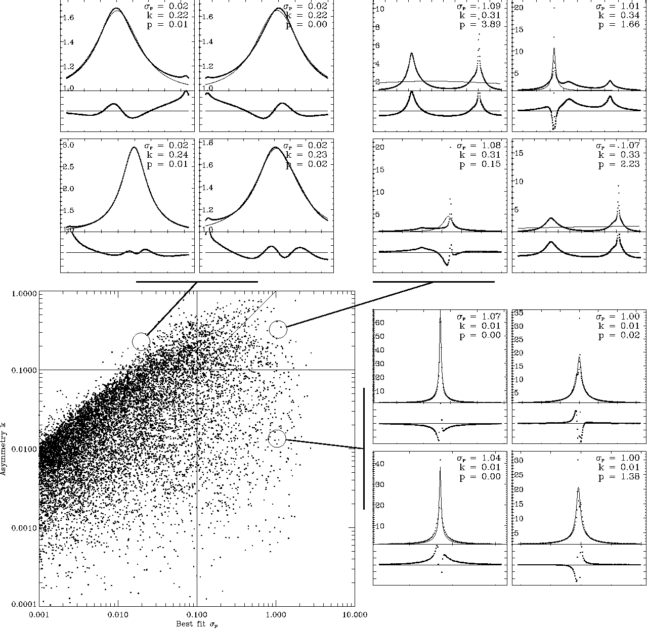
Figure 15.— Scatter plot showing the relative distribution of the best-fit parameter $\sigma_{P}$ and the asymmetry parameter $k$. Horizontal and vertical lines denote parameter values of 0.10, and along the diagonal line the two parameters are equal. Note that there are a significant number of light curves for which one parameter is greater than 0.10 but not the other. Sample light curves are shown to represent three different places in the parameter space: above are four curves with significant asymmetry but good point lens fits; right are four symmetric curves without good point lens fits; above and right are four curves with high values of both parameters. Beneath each light curve is shown the residual plot for the best point lens fit. For clarity, this scatter plot shows only one in every 10 points compared with the next two plots.

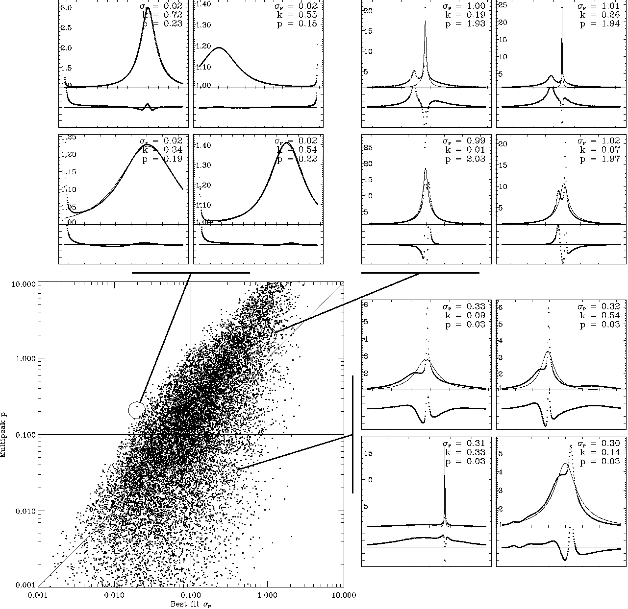
Figure 16.— Scatter plot showing the relative distribution of the best-fit parameter $\sigma_{P}$ and multipeak parameter $p$. Horizontal and vertical lines denote parameter values of 0.10, and along the diagonal line the two parameters are equal. Again, there are a significant number of light curves for which one parameter is greater than 0.10 but not the other. Sample light curves are shown to represent three different places in the parameter space: above are four curves with significant secondary peaks but good point lens fits; right are four curves with only very small secondary peaks, but without good point lens fits; above and right are four curves with high values of both parameters. Beneath each light curve is shown the residual plot for the best point lens fit. Single-peaked events have $p=0$ and so are not represented in this scatter plot.

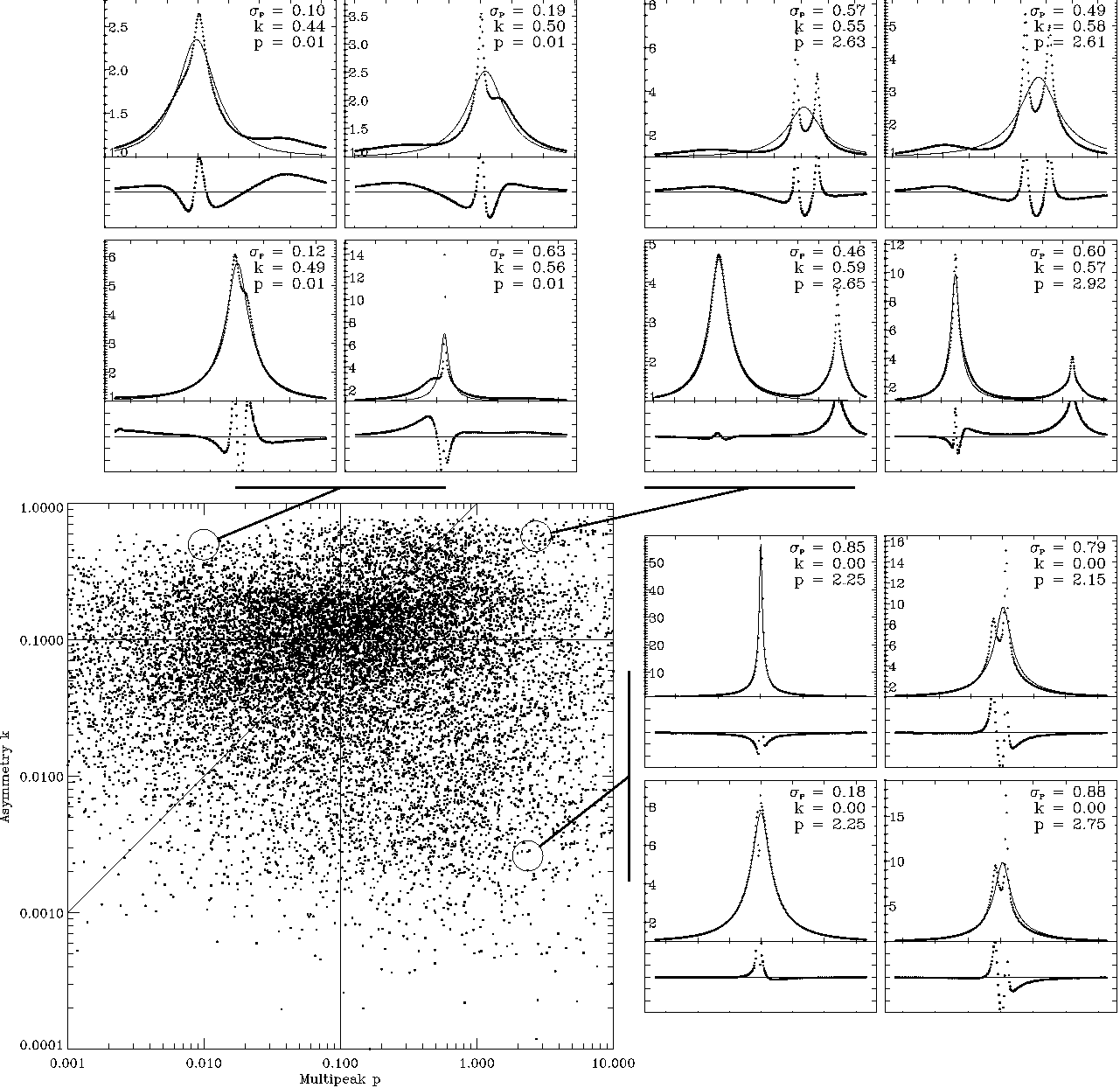
Figure 17.— Scatter plot showing the relative distribution of the multipeak parameter $p$ and the asymmetry parameter $p$. Horizontal and vertical lines denote parameter values of 0.10, and along the diagonal line the two parameters are equal. Again, there are a significant number of light curves for which one parameter is greater than 0.10 but not the other. Sample light curves are shown to represent three different places in the parameter space: above are four curves with very small secondary peaks but high asymmetry; right are four symmetric curves with significant secondary peaks; above and right are four curves with high values of both parameters. Beneath each light curve is shown the residual plot for the best point lens fit. Single-peaked events have $p=0$ and so are not represented in this scatter plot.

4.4. Additional ways to detect perturbations

In the work presented above we have used the value of $\sigma_{P}$ to determine whether a light curve should be viewed as smoothly perturbed from the point lens form. Other parameters, such as the asymmetry parameter, $k$, and the multipeak parameter, $p$ have been defined and calculated to provide ways of characterizing deviations from the point lens form. It is important to note, however, that by using $\sigma_{P},$ we are employing a measure of the deviation of the light curve as a whole. Light curves with short-lived deviations from the point lens form may not be characterized as smoothly perturbed for values of $\sigma_{P}\sim 0.1,$ even if current observational setups can detect the short-lived deviations at a high level of significance.

In other words, by using $\sigma_{P}$ to identify smoothly perturbed light curves, we are taking a conservative approach. This seems appropriate, given that it has so far been relatively difficult to identify smoothly perturbed light curves in real data sets. Nevertheless, in future work it may be appropriate to extend the definition of smoothly perturbed light curves to include some with small values of $\sigma_{P},$ but large values of $k$ or $p.$

We therefore consider the distribution of the three parameters $\sigma_{P}$, $k$, and $p$ that is produced by the default binary distribution in §4.2. We consider the parameters independently (Figure 14) and also in relation to one another (Figures 15 through 17). These figures suggest that it would be worthwhile to augment least squares fitting by considering other avenues of identifying binary lens events. If this is done, some events that would otherwise be classified as point lens like will instead be classified as smoothly perturbed. The predicted values of $\langle s_{sp}\rangle/\langle s_{cc}\rangle$ would then be even larger.

5. Conclusions

We have explored and categorized the full range of microlensing light curves produced by binary lenses. The three mutually exclusive categories of binary lens light curves we have studied are point lens like, smoothly perturbed, and caustic crossing. Smoothly perturbed light curves are defined to be those that exhibit continuous deviations from the point lens form; this naturally excludes caustic crossings. In this paper, smoothly perturbed light curves have been identified by their failure to be fit by a point lens model with a least squares metric. We have also determined whether each light curve we have computed exhibits asymmetry with respect to time reversal, and/or multiple peaks. For the purposes of this paper, we have used an asymmetry parameter and a multipeak parameter only to characterize the deviations from the point lens form, not to identify smoothly perturbed light curves.

Because we have sampled a wide range of binary separations, we have also covered repeating events (Di Stefano & Mao, 1996). Our simulation results are consistent with the analytically calculated rates (Di Stefano & Scalzo, 1999b) and predict that repeating events will form a significant part of data sets that are sensitive to deviations at the few percent level. The rate of repeating events increases with the size of the lensing region, and so it increasing significantly with improved photometric precision. The sensitivity of existing data sets should be enough for repeating events to constitute a few percent of binary lens events, so as the number of binary events approaches 100 and sensitivity continues to improve, repeating events become inevitable.

As with repeating events, other types of exotic events that are expected to constitute just a few percent of binary lens events will also become inevitable with growing data sets.

5.1. The missing smoothly perturbed light curves

Our most striking result relates to the relative number of caustic crossing events. We find that under most assumptions about the binary lens population and about the observational sampling, there should be more smoothly perturbed events than caustic crossing events. This is in contrast to the observational results to date, in which binary lens events are dominated by caustic crossing events.

To determine the reasons for this discrepancy, we have conducted a range of simulations. We find that the ratio is not very sensitive to changes in the binary population, specifically the distribution of binary parameters. The reason for the discrepancy must therefore be related to the observational setup or to the analysis. We also find, however, that the ratio is not very sensitive to changes in the cutoff magnification or sampling frequency. It is of course sensitive to changes in the photometric uncertainty, but it would have to be much larger than $10\%$ to account for the discrepancy. Note that we have considered only the case in which the fractional photometric uncertainties are constant. On the other hand, the observational uncertainties near peaks in magnification may tend to be smaller. If so, for a given value of the uncertainty at baseline, more deviations from the point lens form could be observed. This would further increase the fraction of events that are recognized as being smoothly perturbed.

Is it possible that some of the physical effects we have neglected in our simulations could produce more caustic crossing events and fewer smoothly perturbed events? The effects we have neglected include binary rotation, finite source size effects, binary sources, and parallax. All of these effects can produce perturbations from the point lens form. Only rotation is likely to lead to more caustic crossings, and this is expected to happen only rarely. Therefore, calculations that include all of the expected physical effects will likely produce even larger rate ratios.

Only one physical effect seems to have a significant influence, and that is blending. Blending cannot obscure the wall-like features that mark caustic crossings, but it can smooth out the distinctive features of a smoothly perturbed event, making it more likely that a point lens fit will be successful. Blending is therefore expected to decrease the ratio $\langle s_{sp}\rangle/\langle s_{cc}\rangle$. Nevertheless, blending would have to be severe, with only $\sim 12\%$ of the baseline light coming from the lens star, in order for blending to be responsible for the discrepancy between the predictions and the results derived so far. Furthermore, because the present generation of monitoring programs uses image differencing, which mitigates the effects of blending, this cannot explain why recent results still seem to favor caustic crossings (Jaroszynski et al., 2006).

5.2. Searching for the missing events

The discussion above indicates that the lensing programs are likely to have detected smoothly perturbed binary lens light curves, which were not identified as such. Instead, some smoothly perturbed events may have been identified and published as point lens light curves. If this were the case for all smoothly perturbed light curves, then the experimentally derived lensing event rate would be correct, but it would be difficult to assess the contributions of binary lenses.

On the other hand, the perturbations of some smooth binary lens light curves may be so pronounced that they have prevented the events from being identified as lensing candidates at all (Di Stefano & Perna, 1997). This was especially likely during the early phase of microlensing studies, when it was important for selection criteria to be conservative, to be certain that the selected events were truly associated with microlensing.

There are several important reasons to attempt to identify all binary lens events. The first is to make reliable measurements of the optical depth. Beyond the direct considerations of determining the rate of events, the interpretation of the events can help to determine the locations of significant populations of lenses. Already several binary lenses in the direction of the Magellanic clouds have been located by the caustic crossing events they caused. As these events with measurable lens distances are only a fraction of all events caused by the lens population, a large number of all lenses can be located indirectly. Di Stefano (2000) used this argument to demonstrate the possibility that most of the Magellanic Cloud events were caused by self-lensing. To confirm or refute this argument, we must be able to identify the smoothly perturbed binary lens light curves.

The second reason it is important to identify all binary lens events is to learn about the characteristics of the binary lens and planet lens populations. One important strength of microlensing planet searches is that, of all methods of planet and binary detection, microlensing alone can identify the locations and measure some of the properties of planets in distant stellar systems such as external galaxies. To conduct a genuine population study, however, we must be able to identify a wide range of events, and to understand the detection efficiencies for each type of event.

5.3. Future monitoring programs

The ability of monitoring programs to detect lensing events has increased dramatically since the first published events. The OGLE team now routinely identifies roughly 500 lensing events per year, compared with a total of 9 events identified in its first two years (Udalski et al., 1994). New monitoring projects will be focused on microlensing, while wide field monitoring conducted by Pan-STARRS (Kaiser et al., 2002) and LSST (Tyson, 2002) will identify thousands of events per year caused by lenses in the source galaxies, nearby lenses, and also by MACHOs, should they exist (Di Stefano, 2007). The photometric sensitivity of these projects will approach the level of $1\%$. As illustrated in Figure 9, this means that these programs should be able to identify about three times as many smoothly perturbed binary lens light curves as caustic crossing light curves, using least squares fitting alone. If, in addition, pronounced asymmetries or correlated residuals can be used to quantify the probability that some light curves with acceptable point lens fits were caused by binaries, smoothly perturbed light curves may play an even larger role in the data sets.

In order for future monitoring projects to place constraints on the form of dark matter in MACHOs and to study the underlying characteristics of each lens population, including planet lenses, methods to detect the full range of binary lens and planet light curves must be developed, and the relevant detection efficiencies must be quantified.

Acknowledgements: RD would like to thank Rosalba Perna and Nada Petrovic for conversations. Funded in part by NASA NAG5-10705, PHY05-51164, and a grant for SAO Internal Research & Development.

References

- Alcock et al. (2000) Alcock, C., Allsman, R. A., Alves, D., Axelrod, T. S., et al. 2000, ApJ, 541, 270
- Asada et al. (2004) Asada, H., Kasai, T., & Kasai, M. 2004, Progress of Theoretical Physics, 112, 241
- Di Stefano (2000) Di Stefano, R. 2000, ApJ, 541, 587
- Di Stefano (2007) Di Stefano, R. 2007, in preparation
- Di Stefano & Mao (1996) Di Stefano, R., & Mao, S. 1996, ApJ, 457, 93
- Di Stefano & Perna (1997) Di Stefano, R., & Perna, R. 1997, ApJ, 488, 55
- Di Stefano & Scalzo (1999a) Di Stefano, R., & Scalzo, R. A. 1999a, ApJ, 512, 564
- Di Stefano & Scalzo (1999b) —. 1999b, ApJ, 512, 579
- Dominik (1998) Dominik, M. 1998, A&A, 329, 361
- Duquennoy & Mayor (1991) Duquennoy, A., & Mayor, M. 1991, A&A, 248, 485
- Einstein (1936) Einstein, A. 1936, Science, 84, 506
- Erdl & Schneider (1993) Erdl, H., & Schneider, P. 1993, A&A, 268, 453
- Gould & Loeb (1992) Gould, A., & Loeb, A. 1992, ApJ, 396, 104
- Jaroszynski et al. (2006) Jaroszynski, M., Skowron, J., Udalski, A., Kubiak, M., et al. 2006, Acta Astronomica, 56, 307
- Jaroszynski et al. (2004) Jaroszynski, M., Udalski, A., Kubiak, M., Szymanski, M., et al. 2004, Acta Astronomica, 54, 103
- Kaiser et al. (2002) Kaiser, N., Aussel, H., Burke, B. E., Boesgaard, H., et al. 2002, in Presented at the Society of Photo-Optical Instrumentation Engineers (SPIE) Conference, Vol. 4836, Survey and Other Telescope Technologies and Discoveries. Edited by Tyson, J. Anthony; Wolff, Sidney. Proceedings of the SPIE, Volume 4836, pp. 154-164 (2002)., ed. J. A. Tyson & S. Wolff, 154–164
- Mao & Paczynski (1991) Mao, S., & Paczynski, B. 1991, ApJ, 374, L37
- Petters et al. (2001) Petters, A. O., Levine, H., & Wambsganss, J. 2001, Singularity theory and gravitational lensing (Singularity theory and gravitational lensing / Arlie O. Petters, Harold Levine, Joachim Wambsganss. Boston : Birkhäuser, c2001. (Progress in mathematical physics ; v. 21))
- Press et al. (1992) Press, W. H., Teukolsky, S. A., Vetterling, W. T., & Flannery, B. P. 1992, Numerical recipes in FORTRAN. The art of scientific computing (Cambridge: University Press, —c1992, 2nd ed.)
- Schneider et al. (1992) Schneider, P., Ehlers, J., & Falco, E. E. 1992, Gravitational Lenses (Gravitational Lenses, XIV, 560 pp. 112 figs.. Springer-Verlag Berlin Heidelberg New York. Also Astronomy and Astrophysics Library)
- Tyson (2002) Tyson, J. A. 2002, in Presented at the Society of Photo-Optical Instrumentation Engineers (SPIE) Conference, Vol. 4836, Survey and Other Telescope Technologies and Discoveries. Edited by Tyson, J. Anthony; Wolff, Sidney. Proceedings of the SPIE, Volume 4836, pp. 10-20 (2002)., ed. J. A. Tyson & S. Wolff, 10–20
- Udalski et al. (1994) Udalski, A., Szymanski, M., Stanek, K. Z., Kaluzny, J., et al. 1994, Acta Astronomica, 44, 165