Sterile neutrino oscillations after first MiniBooNE results
Abstract
In view of the recent results from the MiniBooNE experiment we revisit the global neutrino oscillation fit to short-baseline neutrino data by adding one or two sterile neutrinos with eV-scale masses to the three Standard Model neutrinos, and for the first time we consider also the global fit with three sterile neutrinos. Four-neutrino oscillations of the (3+1) type have been only marginally allowed before the recent MiniBooNE results, and become even more disfavored with the new data (at the level of ). In the framework of so-called (3+2) five-neutrino mass schemes we find severe tension between appearance and disappearance experiments at the level of more than , and hence no satistfactory fit to the global data is possible in (3+2) schemes. This tension remains also when a third sterile neutrino is added, and the quality of the global fit does not improve significantly in a (3+3) scheme. It should be noted, however, that in models with more than one sterile neutrino the MiniBooNE results are in perfect agreement with the LSND appearance evidence, thanks to the possibility of CP violation available in such oscillation schemes. Furthermore, if disappearance data are not taken into account (3+2) oscillations provide an excellent fit to the full MiniBooNE spectrum including the event excess at low energies.
I Introduction
Recently first results from the MiniBooNE (MB) experiment MB ; MB-talk at Fermilab have been released on a search for appearance with a baseline of 540 m and a mean neutrino energy of about 700 MeV. The primary purpose of this experiment is to test the evidence of transitions reported by the LSND experiment at Los Alamos Aguilar:2001ty with a very similar range. Reconciling the LSND signal with the other evidence for neutrino oscillations is a long-standing challenge for neutrino phenomenology, since it requires a mass-squared difference at the scale, at odd with the values needed to explain atmospheric sk-atm , long-baseline accelerator Aliu:2004sq ; Michael:2006rx , solar sol-radiochem ; SK-solar ; sno , and long-baseline reactor kamland neutrino data.
It turns out that introducing a fourth (sterile) neutrino sterile does not lead to a satisfactory description of all data in terms of neutrino oscillations Maltoni:2002xd ; strumia because of tight constraints from atmospheric sk-atm , solar sno , and null-result short-baseline (SBL) experiments karmen ; Astier:2003gs ; Dydak:1983zq ; Declais:1994su (see Ref. early for early four-neutrino analyses considering LSND, and Refs. Maltoni:2004ei ; Gonzalez-Garcia:2007ib for recent updates). So-called (2+2) schemes are ruled out by strong constraints on a sterile neutrino component in solar as well as in atmospheric neutrino oscillations sol-atm-4nu at high significance. Therefore, we will not consider such schemes in the following. Also (3+1) schemes suffer from a well-known tension between the LSND appearance signal and null-result SBL disappearance experiments Bilenky:1996rw ; Okada:1996kw ; Barger:1998bn ; Bilenky:1999ny ; Peres:2000ic ; Grimus:2001mn ; cornering . We will show that recent MB results further aggravate this tension and hence (3+1) schemes get even more disfavoured. In Ref. Sorel:2003hf a five-neutrino mass scheme of the (3+2) type has been considered, arguing that the disagreement between LSND and null-result experiments becomes somewhat relaxed compared to (3+1), see also Ref. Peres:2000ic . Here we reconsider this possibility in view of the recent MB data. Furthermore, we investigate the impact of adding a third sterile neutrino on the quality of the global fit. Since we know that there are three active neutrinos, the possibility of three sterile neutrinos is appealing for aesthetical reasons.
Apart from sterile neutrino oscillations, various more exotic explanations of the LSND signal have been proposed, for example, neutrino decay Ma:1999im ; Palomares-Ruiz:2005vf , CPT violation cpt ; strumia , violation of Lorentz symmetry lorentz , a lepton number violating muon decay LNV , CPT-violating quantum decoherence Barenboim:2004wu , mass-varying neutrinos MaVaN , or shortcuts of sterile neutrinos in extra dimensions Pas:2005rb .
In this work we concentrate on the oscillation framework including one or more sterile neutrinos at the eV scale. Such models do have an impact on cosmology Cirelli:2004cz . First, the sterile neutrinos will contribute to the effective number of neutrino species at Big Bang nucleosynthesis sterileBBN ; Okada:1996kw , and second, these models are subject to strong bounds on the sum of the neutrino masses in the sub-eV range from the combination of various cosmological data sets (see e.g., Ref. cosmo-bounds for recent analyses). In order to reconcile such neutrino schemes with cosmology some non-standard scenario has to be invoked, see for example Refs. L-asymm ; BBN-majoron ; Gelmini:2004ah .
The outline of the paper is as follows. In Sec. II we consider (3+1) four-neutrino schemes, and give some details on the used data and their analysis. Sec. III is devoted to (3+2) five-neutrino schemes, discussing the compatibility of LSND and MB in such schemes, as well as the problems of these models to reconcile appearance and disappearance experiments. In Sec. IV we extend the (3+2) scheme by adding a third sterile neutrino to a (3+3) six-neutrino model and investigate whether the global fit improves significantly. We summarise in Sec. V. In appendix A we discuss the mechanism to reconcile LSND and MB by CP violation in (3+2) schemes, appendix B contains a parameter counting of general sterile neutrino oscillation schemes, and in appendix C we consider details of the analysis of atmospheric neutrino data in such models.
II (3+1) four-neutrino mass schemes
The (3+1) four-neutrino spectra are a small perturbation to the standard three-active neutrino case. A cluster of three neutrino mass states accounts for the “solar” () and “atmospheric” () mass splittings. The fourth mass state is separated by an eV-scale mass gap to account for the LSND oscillations, and there is only small mixing of active neutrinos with this mass eigenstate.
II.1 Appearance data in (3+1) schemes
We start our discussion of the (3+1) mass scheme by considering the SBL appearance experiments in the (or ) channel, including the LSND Aguilar:2001ty evidence, the bounds from KARMEN karmen and NOMAD Astier:2003gs , and the recent MB MB data. A combined analysis of LSND and KARMEN can be found in Ref. Church:2002tc . In the approximation , the SBL appearance probability in (3+1) schemes is equivalent to the two-neutrino case, where the effective mixing angle is determined by . Therefore, the analysis performed by the MB collaboration MB ; MB-talk directly applies to (3+1) schemes. We comment only briefly on this case, with the main purpose to check our analysis against the official MB results.
For our re-analysis of LSND we fit the observed transition probability (total rate) plus 11 data points of the spectrum with free normalisation, both derived from the decay-at-rest data Aguilar:2001ty . For KARMEN the data observed in 9 bins of prompt energy as well as the expected background karmen is used in the fit. Further details of our LSND and KARMEN analyses are given in Ref. Palomares-Ruiz:2005vf . For NOMAD we fit the total rate using the information provided in Ref. Astier:2003gs ; our exclusion curve is in good agreement with the result presented in that reference.
The MB re-analysis is based on the neutrino flux, efficiencies, and energy resolution provided in Ref. MB-talk , folded with the charged-current quasi-elastic (CCQE) cross section, to obtain a prediction for the CCQE event excess from oscillations. We calibrate our simulation to the official MB analysis using the prediction for two example points provided in Ref. MB . For the fit the spectrum of excess events binned in reconstructed neutrino energy from Fig. 2 of Ref. MB is used, where the error bars include statistical errors and the uncertainty from the background prediction. Detailed technical information the MB oscillation analysis is available at the webpage Ref. MB-data , including efficiencies and error correlations. Our MB results are in good agreement with the official MB analysis as described in that webpage.
MB data are consistent with zero (no excess) above 475 MeV, whereas below this energy a excess of events is observed. Whether this excess comes indeed from transitions or has some other origin is under investigation MB . Lacking any explanation in terms of backgrounds or systematical uncertainties we take these data at face value, and in some cases we will use all 10 bins of the full energy range from 300 MeV to 3 GeV in the fit (“MB300”). However, as discussed in Refs. MB ; MB-talk , two-neutrino oscillations cannot account for the event excess at low energies. We confirm that the quality of the (3+1) MB fit drastically worsens when the two energy bins between 300 and 475 MeV are included in the fit. Therefore, we follow the strategy of the MB collaboration and restrict the (3+1) analysis to the energy range from 475 MeV to 3 GeV (“MB475”).
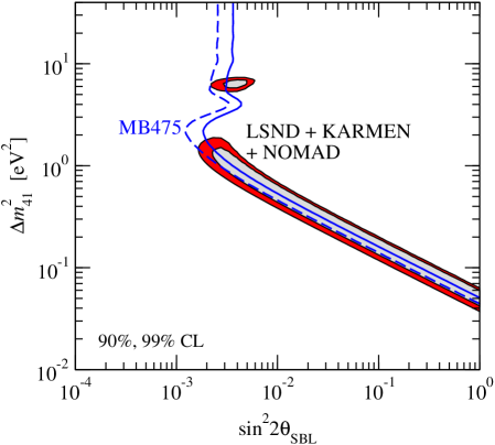
The bound from MB475 data is shown in Fig. 1 in comparison with the allowed region from the combined LSND, KARMEN, NOMAD data. In agreement with Refs. MB ; MB-talk we find that the 90% CL regions do not overlap. A marginal overlap appears if both data sets are stretched to the 99% CL. If all data are summed we find a best fit point with for degrees of freedom (dof). Although this leads to a very good nominal goodness-of-fit (gof), the figure clearly shows that there is significant tension between MB and LSND. A powerful tool to evaluate the compatibility of different data sets is the so-called parameter goodness-of-fit (PG) criterion discussed in Ref. Maltoni:2003cu . It is based on the function
| (1) |
where is the minimum of all data sets combined and is the minimum of the data set . This function measures the “price” one has to pay by the combination of the data sets compared to fitting them independently. It should be evaluated for the number of dof corresponding to the number of parameters in common to the data sets, see Ref. Maltoni:2003cu for a precise definition. Applying this test to check the compatibility of MB with the other SBL appearance data, we find (2 dof), corresponding to a PG of 2.5%. If we test the compatibility of the three data sets MB, LSND, and KARMEN+NOMAD we find (4 dof), and . In the latter case the slight tension between LSND and KARMEN also contributes to the , whereas in the first case this tension is removed since they are added into one single data set.
II.2 Global SBL data in (3+1) schemes
Now we proceed to the global four-neutrino analysis, adding also the information from disappearance experiments. We include the Bugey Declais:1994su , Chooz Apollonio:2002gd , and Palo Verde Boehm:2001ik reactor experiments, as well as the CDHS Dydak:1983zq disappearance experiment. Details of our Bugey and CDHS fits can be found in Ref. Grimus:2001mn . Furthermore, atmospheric neutrino data give an important constraint on the parameter Bilenky:1999ny ; cornering , which is equal to in (3+1) schemes, see Ref. MSV-4nu and appendices B, C. This information is crucial for the region of , where the bound from CDHS disappears. We use the updated atmospheric neutrino analysis from Ref. Gonzalez-Garcia:2007ib , which includes also recent K2K Aliu:2004sq and MINOS Michael:2006rx data, and include the bound on as one single data point in the SBL fit. The total number of data points in the (3+1) analysis is
| (2) |
It is well known that (3+1) schemes suffer from a tension between the LSND appearance signal and the bounds from disappearance experiments, see, e.g., Refs. Bilenky:1996rw ; Okada:1996kw ; Barger:1998bn ; Bilenky:1999ny ; Peres:2000ic ; Grimus:2001mn . Reactor experiments constrain the parameter , CDHS and atmospheric neutrinos limit , whereas the LSND oscillation amplitude is given by . Because of this tension (3+1) schemes have been already disfavoured before the recent MB results, see Ref. Maltoni:2004ei . Testing the compatibility of LSND with all the no-evidence experiments (NEV) without MB leads to a for 2 dof, which indicates an inconsistency at high CL. Since MB475 data is also in conflict with the LSND signal the new data adds to the tension and we find
| (3) |
Alternatively one may test the compatibility of the three data sets LSND, MB475+KARMEN+NOMAD (NEV-APP), and disappearance experiments, which gives
| (4) |
These numbers formally imply inconsistency at more than , and hence we conclude that (3+1) schemes are highly disfavoured by recent data. This level of incompatibility is already close to the one of solar and atmospheric neutrino data in (2+2) four-neutrino schemes Maltoni:2002xd ; Maltoni:2004ei ; Gonzalez-Garcia:2007ib with a (1 dof). Let us mention that the global best fit point of all data has for dof, which nominally gives an excellent gof. However, in the standard gof test the problems in the fit get diluted by the large number of data points, and the disagreement of different data sets becomes only visible when they are analysed separately and then compared to each other, see Ref. Maltoni:2003cu for a detailed discussion.

The bound from NEV data in comparison with the LSND region is shown in Fig. 2. Let us mention that the shape of the NEV bound does hardly change by adding MB data, however the of the global best fit point increases significantly (see above). Note also, that for our LSND analysis we use only the decay-at-rest data, where the appearance signal is most significant.111The LSND allowed region of Fig. 2 consists of a connected band, which shows that the fit is dominated by the total rate and the spectral information available to us is not strong enough to produce disconnected regions as obtained from an event-based likelihood analysis Church:2002tc . However, the location and size of our region are in very good agreement with Ref. Church:2002tc , and moreover, the regions of the parameter space which are relevant for the combination with NEV data are reproduced very well. If the global LSND data including also the decay-in-flight events are used, the LSND regions shift to slightly smaller values of and the disagreement with NEV gets somewhat less severe, see Ref. Maltoni:2002xd for a discussion of this issue.
III (3+2) five-neutrino mass schemes
Five-neutrino schemes of the (3+2) type are a straight-forward extension of (3+1) schemes. In addition to the cluster of the three neutrino mass states accounting for “solar” and “atmospheric” mass splittings now two states at the eV scale are added, with a small admixture of and to account for the LSND signal. In Ref. Sorel:2003hf it has been argued that in (3+2) schemes the tension between LSND and NEV data becomes significantly relaxed compared to the (3+1) case. Here we reconsider this possibility in the light of the new MB data.
III.1 Appearance data in (3+2) schemes
First we consider appearance data only (LSND, KARMEN, NOMAD, and MB). In the SBL approximation , the relevant appearance probability is given by
| (5) |
with the definitions
| (6) |
Eq. (5) holds for neutrinos (NOMAD and MB); for anti-neutrinos (LSND and KARMEN) one has to replace . Since Eq. (5) is invariant under the transformation and , we can restrict the parameter range to , or equivalently , without loss of generality. Note also that the probability Eq. (5) depends only on the combinations and , and therefore, the total number of independent parameters is 5 if only appearance experiments are considered.
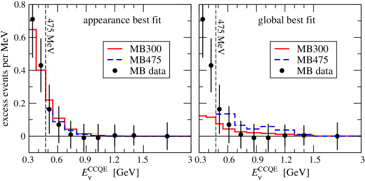
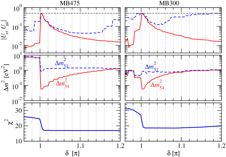
Non-trivial values of the complex phase lead to CP violation, and hence in (3+2) schemes much more flexibility is available to accommodate the results of LSND (anti-neutrinos) and MB (neutrinos).222The possibility to use CP violation to reconcile LSND with a possible null-result of MB neutrino data was pointed out in Ref. Palomares-Ruiz:2005vf in the framework of neutrino decay, and later in Ref. Karagiorgi:2006jf in relation with (3+2) oscillations. Indeed we find that MB is perfectly compatible with LSND in the (3+2) framework. In Fig. 3 (left) we show the prediction for MB at the best fit points in the combined MB, LSND, KARMEN, NOMAD analysis. Clearly MB data can be fitted very well by simultaneously explaining the LSND evidence; we have checked that the prediction for the LSND oscillation probability is within the range of the observed value. In this case also the low energy MB data can be explained, and therefore, in contrast to (3+1) schemes, (3+2) oscillations offer an appealing possibility to account for this excess. In the following we will present results from both MB data sets, MB475 as well as MB300. Note that for MB475 the number of data points used in our analysis is given in Eq. (2), whereas for the case of MB300 two more data points should be added to and . The parameter values and the minima at the best fit points are given in Tab. 1. In both cases, MB475 and MB300, a gof of 85% is obtained, showing that MB is in very good agreement with global SBL appearance data including LSND.
| data set | gof | ||||||||
|---|---|---|---|---|---|---|---|---|---|
| appearance (MB475) | 0.044 | 0.66 | 0.022 | 1.44 | 1.12 | 85% | |||
| appearance (MB300) | 0.31 | 0.66 | 0.27 | 0.76 | 1.01 | 85% | |||
| global data (MB475) | 0.11 | 0.16 | 0.89 | 0.12 | 0.12 | 6.49 | 1.64 | 63% | |
| global data (MB300) | 0.12 | 0.18 | 0.87 | 0.11 | 0.089 | 1.91 | 1.44 | 41% | |
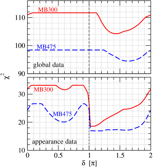
In Fig. 4 (bottom) the is shown as a function of the CP phase . The data prefer values in the range in order to reconcile LSND and MB. However, as visible in the figure no pronounced minimum appears and a rather broad range of values lead to a good fit, including also values rather close to the CP conserving value . For MB300 the best fit even occurs at , compare Tab. 1. In appendix A we give an explanation how LSND and MB can be reconciled with values of that close to . As discussed there, this mechanism is based on a delicate interplay of the three terms in the probability of Eq. (5), and a “tiny amount of CP violation” suffice to make LSND and MB compatible. However, this mechanism requires rather large values of the appearance amplitudes and , which are not compatible with disappearance data, and hence solutions with close to are not possible in the global fit (see upper panel of Fig. 4 and the discussion in the following subsection).
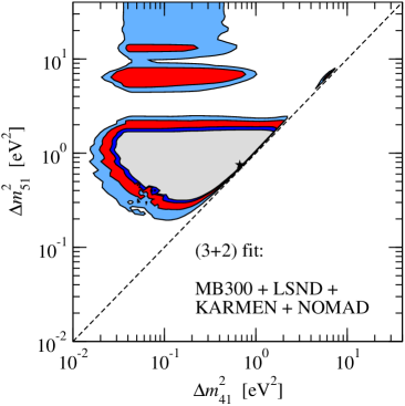
The allowed range in the plane of the two mass-squared differences is shown in Fig. 5. Again we observe that the solution is not particularly fine-tuned and a rather wide 90% CL region appears. The fit using MB300 is somewhat more constrained by the requirement to fit the low energy excess in MB. The fact that for MB300 the best fit occurs for is not statistically significant; the allowed region extends far into the hierarchical regime.
III.2 Global SBL data in (3+2) schemes
Now we proceed to the global analysis in (3+2) schemes, to see whether the successful description of all appearance data found in the previous sub-section can be reconciled also with the bounds from disappearance experiments. The (3+2) survival probability in the SBL approximation is given by
| (7) |
where is given in Eq. (6). Similar as in the (3+1) case, also for (3+2) schemes atmospheric neutrino data provide an important constraint on oscillations with sterile neutrinos. The five-neutrino atmospheric neutrino analysis is discussed in detail in the appendices B and C. It turns out that the same constraint as in the four-neutrino case applies, where now the definition has to be used (see appendix B).
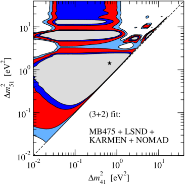
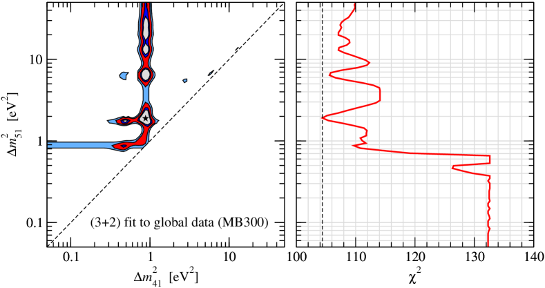
The results of our global (3+2) fit are summarised in the lower part of Tab. 1, where the parameter values, the and the gof of the best fit points are given, again for both MB options, MB475 and MB300. The allowed regions for the global fit in the plane of the mass-squared differences are shown in Figs. 6 and 7.
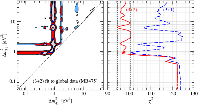
In the right panel of Fig. 6 we show the projections for (3+1) and (3+2) schemes. Comparing the two best fit points provides a method to assess the relative quality of the fit in the two models (likelihood ratio test). We find that introducing the second sterile neutrino leads to the relative improvement of the fit of
| (8) |
where the number of dof corresponds to the additional 4 parameters introduced by moving from (3+1) to (3+2). Hence, (3+1) can be rejected only at the 81% CL with respect to the (3+2) model. This explains also the “stripes” at and around , which appear at 99% CL in Fig. 6. They correspond to the (3+1) solution, which is always present as limiting case in (3+2). Also note, that in the case of appearance data alone we find
| (9) |
Comparing this number with Eq. (8) shows that the main improvement in (3+2) schemes is to reconcile LSND and MB, whereas it is not possible to evade efficiently the constraints from disappearance data. This result is somewhat in disagreement with the conclusion of Ref. Sorel:2003hf . A possible source of this different result might be the inclusion of atmospheric neutrino data in the fit, which is quite important to constrain sterile oscillations in the sector. Our results are in accordance with the arguments presented in the appendix of Ref. Peres:2000ic .
In the upper panel of Fig. 4 the of the global fit is shown as a function of the complex phase . One can see from that figure that the global data prefer values of close to “maximal” CP violation at . The best fit values are and for MB475 and MB300, respectively. As discussed in appendix A, reconciling MB and LSND with values of very close (as found for appearance data only) requires rather large values of the appearance amplitudes and , close to the upper bound from unitarity. Such large values are not compatible with disappearance data, and hence solutions with close to are not possible in the global fit.
From the values given in Tab. 1 it appears that the model provides a very good fit to the data. However, as in the (3+1) case the problem appears when the compatibility of different data sets is considered. Let us divide the global data into appearance and disappearance experiments and check their compatibility with the PG test Maltoni:2003cu according to Eq. (1). We find the following values, for global data without MB, with MB475, and with MB300:333We have tested this result explicitly with the “official” MB analysis available at Ref. MB-data . Using the MB from that source the PG test for appearance and disappearance data gives (MB475) and 24.6 (MB300), in good agreement with our results displayed in Eq. (10).
| PG | (10) | |||||
| PG | ||||||
| PG |
The PG values have been calculated for 4 dof Maltoni:2003cu . This number corresponds to the four independent parameter (combinations) , representing the minimal number of parameter (combinations) in common to the two data sets. From Eq. (10) we conclude that also in (3+2) schemes a severe tension exists between appearance and disappearance experiments. If MB475 is used the result is very similar to the situation without MB data implying inconsistency at about , whereas in case of the full MB data the tension becomes significantly worse (about ), since appearance data are more constraining because of the need to accommodate LSND as well as the MB excess at low energies.
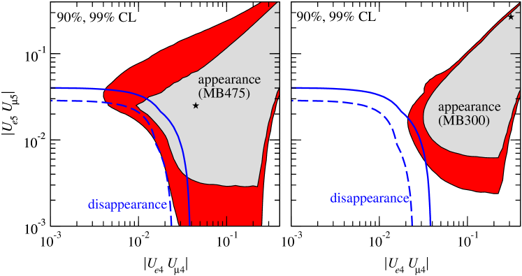
The tension between appearance and disappearance data is illustrated in Fig. 8, where we show the projections of the allowed regions in the plane of the appearance amplitudes and . The opposite trend of the two data sets is clearly visible, especially when the low energy excess in MB is included (right panel). Note that an overlap of the regions visible in that figure does not prove that there is indeed an overlap of the allowed regions in the full parameters space since only a projection is shown. The “common” values in the plane shown in the plot might correspond actually to different locations in the space of and . However, if no overlap is visible in that projection at a certain CL there is also no overlap at that CL in the full parameter space.
Comparing the numbers for MB475 and MB300 given in Eq. (10) it becomes obvious that the MB low energy excess is a severe problem in the global (3+2) fit, although a very good fit can be obtained for appearance data only. This is also apparent from the values given in Tab. 1: Adding the two additional MB data points at low energy leads to an increase of the best fit of about 10 units from 94.5 to 104.4. Indeed, using the global data the MB excess cannot be fitted, as visible in the right panel of Fig. 3, where we show the prediction for the MB spectrum at the global best fit point. The reason is that to explain the excess relatively large values of and are required (see Fig. 8, right), which are inconsistent with disappearance data.
Before closing this section we give the results of an alternative consistency test for the (3+2) model. Instead of dividing the global data into appearance and disappearance experiments, we now consider the two data sets LSND and all the remaining NEV data, similar as done in Eq. (3) and Fig. 2 for the (3+1) schemes. In case of (3+2) this analysis gives
| (11) |
Here 5 dof have been used, corresponding to the 5 parameters in common. Without MB we find in this case , . Hence, the PG test gives a disagreement between LSND and the remaining SBL data similar to the disagreement between appearance and disappearance data found in Eq. (10).
IV (3+3) six-neutrino mass schemes
Since there are three active neutrinos it seems natural to consider also the case of three sterile neutrinos. If all three additional neutrino states have masses in the eV range and mixings as relevant for the SBL experiments under consideration, such a model will certainly have severe difficulties to accommodate standard cosmology cosmo-bounds , and one has to refer to some non-standard cosmological scenario L-asymm ; BBN-majoron ; Gelmini:2004ah . Here we leave this problem aside and focus on neutrino oscillation data, investigating how much the fit improves with respect to the five-neutrino case.
The relevant oscillation probabilities are easily generalised to the (3+3) scheme:
| (12) |
with the definitions
| (13) |
Eq. (12) holds for neutrinos, for anti-neutrinos one has to replace . Note that only two phases are independent. The survival probability is given by
| (14) |
Atmospheric data is included in a similar way as in the previous cases, by using , where now we define , see appendix B. In general, one of the new mass-splittings could also fall into the atmospheric range of few eV2. We have not considered such degenerate situations, and we always assume that all , , with are infinite for the atmospheric neutrino analysis.
We have scanned the of global data in the 11 dimensional parameter space, where a grid of values for the mass-squared differences has been used, spaced logarithmically from 0.1 to 20 eV2. In each point of this grid the remaining 8 parameters have been minimised by a standard optimisation routine.

The results of our search are shown in Fig. 9, where we display the global as a function of . For comparison also the curves in the case of (3+2) and for MB475 also for (3+1) are shown. Note that different from Sec. III, here we do not impose any constraint on the ordering of the mass-squared differences, and the full -dimensional space is scanned for the (3+) scheme. This implies that the result is symmetric with respect to the mass-squared differences, and the functions projected onto any of the -axes () are identical. (Just for convenience we label the horizontal axis in Fig. 9 as , since it is available in all schemes.) Furthermore, as a consequence of this symmetry there are 2 (3) degenerate minima in the five (six) neutrino case, which corresponds to a re-labelling of the mass states. Note also, as it must be, the of the (3+()) model is the maximal value in (3+), since the (3+()) fit is always available as limiting case.
| gof | CL | ||||||
|---|---|---|---|---|---|---|---|
| MB475 | 0.46 | 0.83 | 1.84 | 57% | 20% | ||
| MB300 | 0.46 | 0.83 | 1.84 | 40% | 52% |
The global (3+3) best fit points are summarised in Tab. 2. From the table and Fig. 9 one can see that there is only a marginal improvement of the fit by 1.7 units in for MB475 (3.5 for MB300) with respect to (3+2), to be compared with 4 additional parameters in the model. Hence, we conclude that there are no qualitatively new effects in the (3+3) scheme. The conflict between appearance and disappearance data remains a problem, and the additional freedom introduced by four new parameters does not relax significantly this tension.
V Summary
We have considered the global fit to SBL neutrino oscillation data including the recent data from the MiniBooNE (MB) experiment MB in the framework of four-, five-, and six-neutrino oscillations. We have divided the global data into various sub-sets and tested their consistency within the sterile-neutrino oscillation framework. These results are summarised in Tab. 3 for the (3+1) and (3+2) schemes. Clearly, in all cases we find severe tension between different sub-samples of the data, with the only exception when LSND and the low-energy excess in MB are left out, and in this case indeed no sterile neutrinos are needed and the standard three active neutrino scheme (3+0) provides a perfect fit to the data.
| (3+1) | (3+2) | |||||
|---|---|---|---|---|---|---|
| /dof | /dof | PG | /dof | /dof | PG | |
| DIS vs K+N+L | 95.5/96 | 14.8/2 | 92.1/92 | 17.4/4 | ||
| DIS vs K+N+L+MB475 | 94.5/100 | 17.2/4 | ||||
| DIS vs K+N+L+MB300 | 104.4/102 | 25.1/4 | ||||
| DIS vs K+N+MB475 | 70.5/93 | 0.1/2 | 0.95 | 68.9/89 | 1.1/4 | 0.89 |
| DIS vs K+N+MB300 | 79.1/91 | 10.3/4 | ||||
| NEV vs L | 95.5/96 | 20.9/2 | 92.1/92 | 19.6/5 | ||
| NEV+MB475 vs L | 100.7/104 | 24.7/2 | 94.5/100 | 21.2/5 | ||
Let us summarise our findings:
-
1.
(3+1) four-neutrino schemes are strongly disfavoured because
-
(a)
recent MB data is incompatible with LSND at the 98% CL MB ,
-
(b)
the tension between LSND and NEV SBL data becomes more severe due to MB, there is no overlap of the allowed regions for NEV and LSND at 99% CL, and the PG test implies inconsistency at the level of ,
-
(c)
it is not possible to account for the low energy event excess in MB.
-
(a)
-
2.
(3+2) five-neutrino schemes
-
(a)
do provide a good fit to LSND and the recent MB data,
-
(b)
they can account for the low energy event excess in MB, however
-
(c)
there is significant tension between appearance and disappearance data (according to the PG test at the level of for MB475 and for MB300).
-
(a)
-
3.
(3+3) six-neutrino schemes do not offer qualitatively new effects, the global improves only by about 1.7 (3.5) units for MB475 (MB300) with respect to (3+2), and hence, the conflict between appearance and disappearance data remains.
The points 2a and 2b might be considered as an interesting hint in favour of (3+2) schemes. Since the combined fit of LSND and MB is based on a non-trivial complex phase which introduces a difference in neutrino and anti-neutrino oscillations, these results would represent the first indication of CP violation in neutrino oscillations. This hypothesis could be tested by MB anti-neutrino data, which is currently being accumulated. However, point 2c is a challenge for the (3+2) model. The conclusions of 2c and 3 strongly rely on the disappearance experiments Bugey and CDHS. A crucial check would be the confirmation of or disappearance at the scale. Hence, it might be worth to investigate the possibility to obtain such information at future reactor experiments reactor , from disappearance experiments based on low-energy neutrinos from radio-active sources low-energy , or at the near detector complex of up-coming long-baseline superbeam experiments LBL . A characteristic signal of sterile neutrino oscillations could be obtained at experiments exploring neutral-current detection Garvey:2005pn .
Acknowledgements.
We thank Michel Sorel for communication on the MiniBooNE experiment and useful comments on our analysis. MM is supported by MCYT through the Ramón y Cajal program, by CiCYT through the project FPA2006-01105 and by the Comunidad Autónoma de Madrid through the project P-ESP-00346.Appendix A Reconciling LSND and MB in (3+2) schemes
In this appendix we discuss in some detail how LSND and MB are reconciled in (3+2) schemes exploring CP violation in the appearance probability. In particular, it is intriguing that a very good fit can be obtained with a complex phase very close to the CP conserving value , compare Fig. 4. To understand this effect we show in Fig. 10 a zoom into the region around , and we display in addition to the also the values obtained for the oscillation parameters.
Let us consider the probability given in Eq. (5). A non-trivial possibility to suppress this probability can be obtained by requiring . Then one has
| (15) |
with the abbreviation . Hence, the probability is small for and . This is precisely the behaviour shown in Fig. 10: when approaches from above, becomes small and the approach each other. Writing one has , Eq. (15) is valid, and the oscillation probability is suppressed in MB.
Now the question arises whether large enough values for can be achieved in order to explain LSND. The difference of anti-neutrino and neutrino probabilities is given by
| (16) |
where in the last step has been used. Since and are small, the other factors have to be as large as possible in order to get a sufficient probability for LSND. Indeed, for eV2 one has , and also the grow for (see Fig. 10). Once the maximal values allowed by unitarity, , are reached the LSND probability is given roughly by , where we used (in order to explain MB) and (in order to have ). Using the experimental value one finds that a fit should be possible for , in agreement with our results.
The similar structure of the left and right panels of Fig. 10 suggests that this mechanism works equally well for MB475 and MB300, and fitting the low energy excess in MB does not affect these considerations. Obviously, this explanation is not valid for , since the CP asymmetry Eq. (16) has the wrong sign to reconcile LSND and MB. As visible in Fig. 10, the fit jumps into a quite different solution, which anyway gives a poor . Also, the local minimum around visible in Fig. 4 for MB475 requires a different explanation in order to obtain the correct sign of the CP asymmetry for these values of . Let us also mention that quite large values of and close to the unitarity bound do appear in the fit for , since only appearance experiments are used. Such large values are not possible if disappearance experiments are included, which basically require that each of the , , has to be small. This is one reason for the difficulties in reconciling appearance and disappearance data, in close analogy to (3+1).
Appendix B Oscillations with extra sterile states
In this appendix we discuss in some detail atmospheric and short-baseline neutrino oscillations involving extra sterile neutrino states. For definiteness, we will focus on (3+3) schemes; expressions for (3+2) and (3+1) models can be easily obtained by dropping all terms containing a redundant “6” or “5” index. Let us order the flavor eigenstates as and introduce the following parametrisation for the neutrino mixing:
| (17) |
where represents a complex rotation by an angle and a phase in the plane, while is an ordinary rotation by an angle . Note that rotations involving only sterile states (i.e., with both ) are unphysical, and therefore we have omitted them from Eq. (17). For the general case with sterile states, it is convenient to choose the rotations and as real, and the remaining ones as complex. The matrix then includes angles and phases.
A number of simplifying assumptions can be made in the analysis of short-baseline as well as atmospheric and long-baseline neutrino experiments. For short-baseline experiments one can neglect the solar and atmospheric mass splittings, and . In this approximation, the mixing angles , and disappear from the relevant probabilities. Furthermore, matter effects can be neglected. Since we do not consider neutral current interactions in our analysis, the neutrino is essentially indistinguishable from the sterile states, as it participates neither in the production nor in the detection processes. Therefore, all the angles also disappear. So for (3+3) models we are left with an effective mixing matrix
| (18) |
which contains six angles and two CP phases. In general, under our approximations SBL experiments depend on angles and phases. For example, in (3+2) models we have four angles (, , , ) and one phase (), and the matrix elements , , , , used in Sec. III are combinations of these five parameters.
For atmospheric and long-baseline experiments (K2K and MINOS) we neglect the mixing of with other neutrino states at the LSND mass-squared splittings, justified by the constraint from Bugey. This corresponds to setting all the angles with to zero. In this approximation, the complex phase can be dropped. Therefore, in (3+3) models we are left with an effective mixing matrix
| (19) |
which contains nine angles and four CP phases. As a general rule, in our approximation for ATM and LBL experiments the matrix contains angles and phases.
From Eqs. (18) and (19) it is straightforward to see that for any number of extra sterile states, , atmospheric and short-baseline experiments are connected only through the angles with (or, equivalently, through the parameters with ). Note that in our convention all the non-vanishing CP phases are “private” to either short-baseline (e.g., and ) or atmospheric (e.g., , , and ) experiments.
Let us now focus on the probabilities relevant for the analysis of atmospheric and long-baseline experiments. The Hamiltonian in the flavor basis is:
| (20) |
where is given in Eq. (19), , and . It is convenient to define and . Then we can write:
| (21) |
In order to further simplify the analysis, let us now assume that all the mass-squared differences involving the “heavy” states with can be considered as infinite: for any and . In leading order, the matrix takes the effective block-diagonal form:
| (22) |
where is the sub-matrix of corresponding to the first, second and third neutrino states, and is a diagonal matrix (the matter terms in this block are negligible in the limit of very large ). Consequently, the evolution matrix is:
| (23) |
We are interested only in the elements , , and . Taking into account the block-diagonal form of and the relations and , we obtain:
| (24) |
The expressions for the probabilities, , are straightforward. Defining
| (25) |
we note that and that for , so that . Therefore:
| (26) |
where we have used the fact that the terms containing a factor oscillate very fast, and therefore vanish once the finite energy resolution of the detector is taken into account. In the above expression is the effective probability derived from the Hamiltonian , which has an ordinary three-neutrino term (including the usual charged-current interaction term of the electron neutrino) plus a matter term arising from the sterile part of :
| (27) |
Eqs. (26) and (27) are valid for any number of extra sterile states.
Appendix C Robustness of the ATM+LBL bound on
As discussed in Refs. Bilenky:1999ny ; cornering , the contribution of atmospheric neutrino data to the disappearance data set plays a crucial role in rejecting sterile neutrino models. In this appendix we re-consider the bound on in (3+1) schemes, generalise it to the (3+) case, and investigate the impact of some of the adopted approximations.
C.1 Decoupling electron neutrinos

Let us begin by considering the simplified case and . In this limit, the electron neutrino state is completely decoupled, so that and .444Up to now this approximation has been always adopted in the literature, and in the following Sec. C.2 we are going to relax it for the first time. Eqs. (26) and (27) then reduce to an effective two-neutrino form in the sector:
| (28) | |||
| (29) |
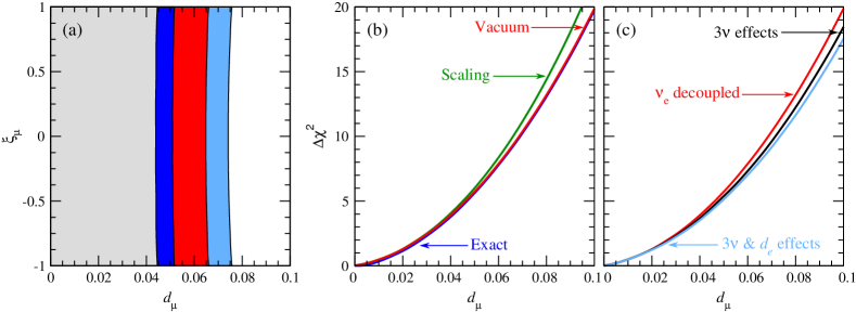
In the case of only one extra sterile state it is possible to perform a full numerical analysis. The details of such an analysis have been widely discussed in Refs. sol-atm-4nu ; MSV-4nu ; Maltoni:2004ei , and are summarised in Fig. 11. As can be seen from this figure, atmospheric and long-baseline neutrino data strongly prefer a pure two-neutrino oscillation scenario, disfavouring both a sterile neutrino contribution to the main oscillations (parametrised by ) and a mixing of with the heavy mass eigenstate (parametrised by ). In this work we are mainly interested in the bound on , since the other parameters are “private” to atmospheric and long-baseline data and can therefore be marginalised.
Let us now turn our attention to five-neutrino models. Even in this case it is possible to perform a full numerical analysis, presented in Fig. 12(a). As mentioned in appendix B, in principle atmospheric and long-baseline data constrain separately and , which we parametrise in terms of and . However, as can be seen from Fig. 12(a) the allowed region is practically independent of . Furthermore, comparing this figure with Fig. 11(c) it turns out that the bound on in four-neutrino and five-neutrino models is practically the same. In other words, the extra freedom which we have in schemes with respect to ones is essentially irrelevant for the constraint on .
In order to understand this result, let us go back to Eqs. (28) and (29) and consider the differences between and models. They arise from two facts:
-
•
In models we have , so that the “scaling” term and the “constant” term in Eq. (28) are related to each other. Conversely, in models , so that the two terms are independent.
-
•
The expression for is different in the two models, due to the different contributions to the sterile matter term in Eq. (29). Again, in five-neutrino models we have more freedom.
The relevance of these differences is illustrated in Fig. 12(b). All the lines correspond to four-neutrino models. The blue line (“Exact”) is the exact bound on from atmospheric and long-baseline data, and coincides with the one shown in Fig. 11(c). The red line (“Vacuum”) is obtained by neglecting the last term in Eq. (29), i.e. by considering only the vacuum part of . Finally, the green line (“Scaling”) is obtained by further neglecting the constant term in Eq. (28), thus setting . As can be seen, sterile-induced matter terms are completely irrelevant for what concerns the bound on , and the constant term in the expression for plays only a minor role. The real bound arises from the scaling term in , which is the same in four-neutrino and five-neutrino models. This explains why the differences between the two schemes are so small. Similarly, the weak dependence on in models arises from the constant term in Eq. (28); in particular, both Figs. 12(a) and 12(b) show that as this term is decreased the quality of the fit gets worse.
In summary, although in principle atmospheric and long-baseline data could constrain separately all the terms in models with extra sterile states, in practice they are only sensitive to the sum of these terms, . Furthermore, the bound on is essentially independent on the number of extra sterile states. The validity of this approximation is crucial for the analysis of (3+3) models, where an exact treatment would be very hard to do due to the large number of parameters involved.
C.2 Including electron neutrinos
In the previous section we have seen that the bound on reflects the ability of atmospheric and long-baseline data to effectively fix the total normalisation of -like events. This is possible in spite of the large normalisation errors (of the order of 20%) on the atmospheric neutrino fluxes and the neutrino-nucleon cross sections, since the accurate measurements of -like neutrino events provided by atmospheric data allows to effectively resolve these uncertainties. In other words, what really matters to determine the bound on is the relative normalisation of -like and -like neutrino events. This opens up the possibility that subleading effects modifying the distribution of electron neutrino data may have a sizable impact on the bound on . In this section we investigate in detail this possibility.
In the context of sterile neutrino schemes there are two types of contributions which affect -like events: (i) “usual” three-neutrino effects induced by or by , and (ii) genuine sterile- effects induced by non-zero (with ). The formalism to study the three-neutrino effects has been developed in appendix B. Following the results of Sec. C.1, we assume that the sterile-induced matter effects in Eq. (27) can be neglected, in which case the effective Hamiltonian and the corresponding probabilities reduce to the usual three-neutrino expressions. Note that again the relevant probabilities are related to the three-neutrino ones only through the parameter , and apart from the “constant” term in the expression for in Eq. (26) (see previous section) these formulas are completely independent from the number of extra sterile species. The results of our analysis are summarised in Fig. 12(c), where we compare the bound for the case when the electron is decoupled (red line) with the same bound including also three-neutrino effects due to and (black line). Note that the Chooz experiment is also included in the fit. As can be seen from this figure, an accurate treatment of subleading three-neutrino effects indeed weakens the bound on , however the effect is very small and has no impact on the conclusions of this work.
Let us now study effects induced by non-zero values of . Following the derivation of appendix B, it is easy to see that in this case and no longer vanish, in which case Eq. (26) should be replaced with expressions involving not only but also interference terms between different entries of . However, it is still true that , so that:
| (30) |
Motivated by this result, we approximate the effects of non-zero by introducing an independent scaling factor for electron events:
| (31) |
If is left free to vary without any constraint, the impact on the bound on is dramatic, since in this case electron events can no longer fix the flux and cross section normalisation uncertainties. However, the value of is strongly bounded by Bugey. We have performed a combined analysis of atmospheric+LBL and SBL data taking into account that both data samples depend on and (using the approximation described above). We find that the final result is practically the same as in our standard case, where the dependence of the ATM data on is neglected. To illustrate this we show in Fig. 12(c), light-blue line, also the bound on from ATM data by adding to the overall a term , which simulates roughly the constraint from Bugey, neglecting that it actually depends on . From this figure it becomes clear that once is limited by the data from Bugey its impact on atmospheric+LBL data is very small.
In conclusion, the atmospheric bound on is robust under our approximations. However, as clear from the above discussion it depends on the assumptions about uncertainties on quantities (like fluxes or cross sections) affecting the ratio of -like and -like atmospheric neutrino event normalisations.
References
- (1) A. A. Aguilar-Arevalo et al. [MiniBooNE Coll.], “A Search for Electron Neutrino Appearance at the Scale,” arXiv:0704.1500 [hep-ex].
-
(2)
W. Louis and J. Conrad [MiniBooNE Coll.], talk at Fermilab, April 11, 2007,
http://www-boone.fnal.gov/publicpages/First_Results.pdf. - (3) A. Aguilar et al. [LSND Coll.], “Evidence for neutrino oscillations from the observation of appearance in a beam,” Phys. Rev. D 64, 112007 (2001) [hep-ex/0104049].
- (4) Y. Fukuda et al. [Super-Kamiokande Coll.], “Evidence for oscillation of atmospheric neutrinos,” Phys. Rev. Lett. 81, 1562 (1998) [hep-ex/9807003]; Y. Ashie et al., “A measurement of atmospheric neutrino oscillation parameters by Super-Kamiokande I,” Phys. Rev. D 71, 112005 (2005) [hep-ex/0501064].
- (5) E. Aliu et al. [K2K Coll.], “Evidence for muon neutrino oscillation in an accelerator-based experiment,” Phys. Rev. Lett. 94, 081802 (2005) [hep-ex/0411038].
- (6) D. G. Michael et al. [MINOS Coll.], “Observation of muon neutrino disappearance with the MINOS detectors and the NuMI neutrino beam,” Phys. Rev. Lett. 97, 191801 (2006) [hep-ex/0607088].
- (7) B. T. Cleveland et al., “Measurement of the solar electron neutrino flux with the Homestake chlorine detector,” Astrophys. J. 496, 505 (1998); J.N. Abdurashitov et al. [SAGE Coll.], “Measurement of the solar neutrino capture rate by the Russian-American gallium solar neutrino experiment during one half of the 22-year cycle of solar activity,” J. Exp. Theor. Phys. 95 (2002) 181 [astro-ph/0204245]; M. Altmann et al. [GNO Coll.], “Complete results for five years of GNO solar neutrino observations,” Phys. Lett. B 616, 174 (2005) [hep-ex/0504037].
- (8) S. Fukuda et al. [Super-Kamkiokande Coll.], “Determination of solar neutrino oscillation parameters using 1496 days of Super-Kamiokande-I data,” Phys. Lett. B 539 (2002) 179 [hep-ex/0205075]; J. Hosaka et al., “Solar neutrino measurements in Super-Kamiokande-I,” Phys. Rev. D 73, 112001 (2006) [hep-ex/0508053].
- (9) Q. R. Ahmad et al. [SNO Coll.], “Direct evidence for neutrino flavor transformation from neutral-current interactions in the Sudbury Neutrino Observatory,” Phys. Rev. Lett. 89, 011301 (2002) [nucl-ex/0204008]; B. Aharmim et al., “Electron energy spectra, fluxes, and day-night asymmetries of B-8 solar neutrinos from the 391-day salt phase SNO data set,” Phys. Rev. C 72, 055502 (2005) [nucl-ex/0502021].
- (10) K. Eguchi et al. [KamLAND Coll.], “First results from KamLAND: Evidence for reactor anti-neutrino disappearance,” Phys. Rev. Lett. 90, 021802 (2003) [hep-ex/0212021]; T. Araki et al., “Measurement of neutrino oscillation with KamLAND: Evidence of spectral distortion,” Phys. Rev. Lett. 94, 081801 (2005) [hep-ex/0406035].
- (11) J. T. Peltoniemi, D. Tommasini and J. W. F. Valle, “Reconciling dark matter and solar neutrinos,” Phys. Lett. B 298, 383 (1993); J. T. Peltoniemi and J. W. F. Valle, “Reconciling dark matter, solar and atmospheric neutrinos,” Nucl. Phys. B 406, 409 (1993) [hep-ph/9302316]; D.O. Caldwell and R.N. Mohapatra, “Neutrino mass explanations of solar and atmospheric neutrino deficits and hot dark matter,” Phys. Rev. D 48, 3259 (1993).
- (12) M. Maltoni, T. Schwetz, M. A. Tortola and J. W. F. Valle, “Ruling out four-neutrino oscillation interpretations of the LSND anomaly?,” Nucl. Phys. B 643, 321 (2002) [hep-ph/0207157].
- (13) A. Strumia, “Interpreting the LSND anomaly: Sterile neutrinos or CPT-violation or…?,” Phys. Lett. B 539, 91 (2002) [hep-ph/0201134].
- (14) B. Armbruster et al. [KARMEN Coll.], “Upper limits for neutrino oscillations from muon decay at rest,” Phys. Rev. D 65, 112001 (2002) [hep-ex/0203021].
- (15) P. Astier et al. [NOMAD Coll.], “Search for oscillations in the NOMAD experiment,” Phys. Lett. B 570, 19 (2003) [hep-ex/0306037].
- (16) F. Dydak et al., “A Search For Muon-Neutrino Oscillations In The Range To ,” Phys. Lett. B 134, 281 (1984).
- (17) Y. Declais et al., “Search for neutrino oscillations at 15-meters, 40-meters, and 95-meters from a nuclear power reactor at Bugey,” Nucl. Phys. B 434, 503 (1995).
- (18) J. J. Gomez-Cadenas and M. C. Gonzalez-Garcia, “Future Tau-Neutrino Oscillation Experiments And Present Data,” Z. Phys. C 71, 443 (1996) [hep-ph/9504246]; S. Goswami, “Accelerator, reactor, solar and atmospheric neutrino oscillation: Beyond three generations,” Phys. Rev. D 55, 2931 (1997) [hep-ph/9507212].
- (19) M. Maltoni, T. Schwetz, M. A. Tortola and J. W. F. Valle, “Status of global fits to neutrino oscillations,” New J. Phys. 6, 122 (2004) [hep-ph/0405172 v5].
- (20) M. C. Gonzalez-Garcia and M. Maltoni, “Phenomenology with massive neutrinos,” arXiv:0704.1800 [hep-ph].
- (21) C. Giunti, M. C. Gonzalez-Garcia and C. Pena-Garay, “Four-neutrino oscillation solutions of the solar neutrino problem,” Phys. Rev. D 62, 013005 (2000) [hep-ph/0001101]; M. C. Gonzalez-Garcia, M. Maltoni and C. Pena-Garay, “Solar and atmospheric four-neutrino oscillations,” Phys. Rev. D 64, 093001 (2001) [hep-ph/0105269]; M. Maltoni, T. Schwetz, M. A. Tortola and J. W. F. Valle, “Constraining neutrino oscillation parameters with current solar and atmospheric data,” Phys. Rev. D 67, 013011 (2003) [hep-ph/0207227].
- (22) S. M. Bilenky, C. Giunti and W. Grimus, “Neutrino mass spectrum from the results of neutrino oscillation experiments,” Eur. Phys. J. C 1, 247 (1998) [hep-ph/9607372].
- (23) N. Okada and O. Yasuda, “A sterile neutrino scenario constrained by experiments and cosmology,” Int. J. Mod. Phys. A 12, 3669 (1997) [hep-ph/9606411].
- (24) V. D. Barger, S. Pakvasa, T. J. Weiler and K. Whisnant, “Variations on four-neutrino oscillations,” Phys. Rev. D 58, 093016 (1998) [hep-ph/9806328].
- (25) S. M. Bilenky, C. Giunti, W. Grimus and T. Schwetz, “Four-neutrino mass spectra and the Super-Kamiokande atmospheric up-down asymmetry,” Phys. Rev. D 60, 073007 (1999) [hep-ph/9903454].
- (26) O. L. G. Peres and A. Y. Smirnov, “(3+1) spectrum of neutrino masses: A chance for LSND?,” Nucl. Phys. B 599, 3 (2001) [hep-ph/0011054].
- (27) W. Grimus and T. Schwetz, “4-neutrino mass schemes and the likelihood of (3+1)-mass spectra,” Eur. Phys. J. C 20, 1 (2001) [hep-ph/0102252].
- (28) M. Maltoni, T. Schwetz and J. W. F. Valle, “Cornering (3+1) sterile neutrino schemes,” Phys. Lett. B 518, 252 (2001) [hep-ph/0107150].
- (29) M. Sorel, J. M. Conrad and M. Shaevitz, “A combined analysis of short-baseline neutrino experiments in the (3+1) and (3+2) sterile neutrino oscillation hypotheses,” Phys. Rev. D 70, 073004 (2004) [hep-ph/0305255].
- (30) E. Ma, G. Rajasekaran and I. Stancu, “Hierarchical four-neutrino oscillations with a decay option,” Phys. Rev. D 61, 071302 (2000) [hep-ph/9908489]; E. Ma and G. Rajasekaran, “Light unstable sterile neutrino,” Phys. Rev. D 64, 117303 (2001) [hep-ph/0107203].
- (31) S. Palomares-Ruiz, S. Pascoli and T. Schwetz, “Explaining LSND by a decaying sterile neutrino,” JHEP 0509, 048 (2005) [hep-ph/0505216].
- (32) H. Murayama and T. Yanagida, “LSND, SN1987A, and CPT violation,” Phys. Lett. B 520, 263 (2001) [hep-ph/0010178]; G. Barenboim, L. Borissov and J. Lykken, “CPT violating neutrinos in the light of KamLAND,” hep-ph/0212116; M. C. Gonzalez-Garcia, M. Maltoni and T. Schwetz, “Status of the CPT violating interpretations of the LSND signal,” Phys. Rev. D 68, 053007 (2003) [hep-ph/0306226]. V. Barger, D. Marfatia and K. Whisnant, “LSND anomaly from CPT violation in four-neutrino models,” Phys. Lett. B 576, 303 (2003) [hep-ph/0308299].
- (33) V. A. Kostelecky and M. Mewes, “Lorentz violation and short-baseline neutrino experiments,” Phys. Rev. D 70, 076002 (2004) [hep-ph/0406255]; A. de Gouvea and Y. Grossman, “A three-flavor, Lorentz-violating solution to the LSND anomaly,” Phys. Rev. D 74, 093008 (2006) [hep-ph/0602237]; T. Katori, A. Kostelecky and R. Tayloe, “Global three-parameter model for neutrino oscillations using Lorentz violation,” Phys. Rev. D 74, 105009 (2006) [hep-ph/0606154].
- (34) K. S. Babu and S. Pakvasa, “Lepton number violating muon decay and the LSND neutrino anomaly,” hep-ph/0204236; B. Armbruster et al. [KARMEN Coll.], “Improved limits on emission from decay,” Phys. Rev. Lett. 90, 181804 (2003) [hep-ex/0302017]; A. Gaponenko et al. [TWIST Coll.], “Measurement of the muon decay parameter delta,” Phys. Rev. D 71, 071101 (2005) [hep-ex/0410045].
- (35) G. Barenboim and N. E. Mavromatos, “CPT violating decoherence and LSND: A possible window to Planck scale physics,” JHEP 0501, 034 (2005) [hep-ph/0404014].
- (36) D. B. Kaplan, A. E. Nelson and N. Weiner, “Neutrino oscillations as a probe of dark energy,” Phys. Rev. Lett. 93, 091801 (2004) [hep-ph/0401099]; K. M. Zurek, “New matter effects in neutrino oscillation experiments,” JHEP 0410, 058 (2004) [hep-ph/0405141]; V. Barger, D. Marfatia and K. Whisnant, “Confronting mass-varying neutrinos with MiniBooNE,” Phys. Rev. D 73, 013005 (2006) [hep-ph/0509163].
- (37) H. Pas, S. Pakvasa and T. J. Weiler, “Sterile – active neutrino oscillations and shortcuts in the extra dimension,” Phys. Rev. D 72, 095017 (2005) [hep-ph/0504096].
- (38) M. Cirelli, G. Marandella, A. Strumia and F. Vissani, “Probing oscillations into sterile neutrinos with cosmology, astrophysics and experiments,” Nucl. Phys. B 708, 215 (2005) [hep-ph/0403158].
- (39) K. Enqvist, K. Kainulainen and M. J. Thomson, “Stringent cosmological bounds on inert neutrino mixing,” Nucl. Phys. B 373, 498 (1992); X. Shi, D. N. Schramm and B. D. Fields, “Constraints on neutrino oscillations from big bang nucleosynthesis,” Phys. Rev. D 48, 2563 (1993) [astro-ph/9307027]; S. M. Bilenky, C. Giunti, W. Grimus and T. Schwetz, “Four-neutrino mixing and big-bang nucleosynthesis,” Astropart. Phys. 11, 413 (1999) [hep-ph/9804421]; P. Di Bari, “Update on neutrino mixing in the early universe,” Phys. Rev. D 65, 043509 (2002); Addendum-ibid. D 67, 127301 (2003) [hep-ph/0108182].
- (40) S. Hannestad and G. G. Raffelt, “Neutrino masses and cosmic radiation density: Combined analysis,” JCAP 0611, 016 (2006) [astro-ph/0607101]; S. Dodelson, A. Melchiorri and A. Slosar, “Is cosmology compatible with sterile neutrinos?,” Phys. Rev. Lett. 97, 04301 (2006) [astro-ph/0511500].
- (41) R. Foot and R. R. Volkas, “Reconciling sterile neutrinos with big bang nucleosynthesis,” Phys. Rev. Lett. 75, 4350 (1995) [hep-ph/9508275]. Y. Z. Chu and M. Cirelli, “Sterile neutrinos, lepton asymmetries, primordial elements: How much of each?,” Phys. Rev. D 74, 085015 (2006) [astro-ph/0608206]; C. J. Smith, G. M. Fuller, C. T. Kishimoto and K. N. Abazajian, “Light element signatures of sterile neutrinos and cosmological lepton numbers,” Phys. Rev. D 74, 085008 (2006) [astro-ph/0608377].
- (42) K. S. Babu and I. Z. Rothstein, “Relaxing nucleosynthesis bounds on sterile-neutrinos,” Phys. Lett. B 275, 112 (1992); L. Bento and Z. Berezhiani, “Blocking active-sterile neutrino oscillations in the early universe with a Majoron field,” Phys. Rev. D 64, 115015 (2001) [hep-ph/0108064].
- (43) G. Gelmini, S. Palomares-Ruiz and S. Pascoli, “Low reheating temperature and the visible sterile neutrino,” Phys. Rev. Lett. 93, 081302 (2004) [astro-ph/0403323].
- (44) E. D. Church, K. Eitel, G. B. Mills and M. Steidl, “Statistical analysis of different searches,” Phys. Rev. D 66, 013001 (2002) [hep-ex/0203023].
-
(45)
Technical data on the MiniBooNE oscillation analysis
is available at the webpage
http://www-boone.fnal.gov/for_physicists/april07datarelease/ - (46) M. Maltoni and T. Schwetz, “Testing the statistical compatibility of independent data sets,” Phys. Rev. D 68, 033020 (2003) [hep-ph/0304176].
- (47) M. Apollonio et al., “Search for neutrino oscillations on a long base-line at the CHOOZ nuclear power station,” Eur. Phys. J. C 27, 331 (2003) [hep-ex/0301017].
- (48) F. Boehm et al., “Final results from the Palo Verde neutrino oscillation experiment,” Phys. Rev. D 64, 112001 (2001) [hep-ex/0107009].
- (49) M. Maltoni, T. Schwetz and J. W. F. Valle, “Status of four-neutrino mass schemes: A global and unified approach to current neutrino oscillation data,” Phys. Rev. D 65, 093004 (2002) [hep-ph/0112103].
- (50) G. Karagiorgi et al., “Leptonic CP violation studies at MiniBooNE in the (3+2) sterile neutrino oscillation hypothesis,” Phys. Rev. D 75, 013011 (2007) [hep-ph/0609177].
- (51) F. Ardellier et al. [Double Chooz Coll.], “Double Chooz: A search for the neutrino mixing angle ,” hep-ex/0606025; X. Guo et al. [Daya Bay Coll.], “A precision measurement of the neutrino mixing angle using reactor antineutrinos at Daya Bay,” hep-ex/0701029.
- (52) C. Giunti and M. Laveder, “Short-baseline active–sterile neutrino oscillations?,” hep-ph/0610352; C. Grieb, J. Link and R. S. Raghavan, “Probing active to sterile neutrino oscillations in the LENS detector,” hep-ph/0611178.
- (53) Y. Itow et al., “The JHF-Kamioka neutrino project,” hep-ex/0106019; D. S. Ayres et al. [NOvA Coll.], “NOvA proposal to build a 30-kiloton off-axis detector to study neutrino oscillations in the Fermilab NuMI beamline,” hep-ex/0503053.
- (54) G. T. Garvey et al., “Measuring active–sterile neutrino oscillations with a stopped pion neutrino source,” Phys. Rev. D 72, 092001 (2005) [hep-ph/0501013].