Chapter 1
Nonlinear Perturbations and Conservation Laws on Curved Backgrounds in GR and other Metric Theories

Abstract

In this paper we review the field-theoretical approach. In this framework perturbations in general relativity as well as in an arbitrary $D$-dimensional metric theory are described and studied. A background, on which the perturbations propagate, is a solution (arbitrary) of the theory. Lagrangian for perturbations is defined, and field equations for perturbations are derived from the variational principle. These equations are exact, equivalent to the equations in the standard formulation and have a form that permits an easy and natural expansion to an arbitrary order. Being covariant, the field-theoretical description is also invariant under gauge (inner) transformations, which can be presented both in exact and approximate forms. Following the usual field-theoretical prescriptions, conserved quantities for perturbations are constructed. Conserved currents are expressed through divergences of superpotentials — antisymmetric tensor densities. This form allows to relate a necessity to consider local properties of perturbations with a theoretical representation of the quasi-local nature of conserved quantities in metric theories. Properties of the conserved quantities under gauge transformations are established and analyzed, this allows to describe the well known non-localization problem in explicit mathematical expressions and operate with them. Applications of the formalism in general relativity for studying 1) the falloff at spatial infinity in asymptotically flat spacetimes, 2) linear perturbations on Friedmann-Robertson-Walker backgrounds, 3) a closed Friedmann world and 4) black holes presented as gravitationally-field configurations in a Minkowski space, are reviewed. Possible applications of the formalism in cosmology and astrophysics are also discussed. Generalized formulae for an arbitrary metric $D$-dimensional theory are tested to calculate the mass of a Schwarzschild-anti-de Sitter black hole in the Einstein-Gauss-Bonnet gravity.

PACS 04.20.Cv, 04.25.Nx, 04.50.+h, 11.30.-j.

1 Introduction and preliminaries

1.1 Perturbations in gravitational theories, cosmology and relativistic astrophysics

Much of research in general relativity (GR) is frequently carried out under the assumption that perturbations of different kinds propagate in a given (fixed) background spacetime (exact solution to the Einstein equations) [1] - [4]. A majority of cosmological and astrophysical problems are also studied in the framework of a perturbation approach. It is quite impossible to give a more or less full bibliography on this topic. Nevetherless, to stress the importance of such studies, we shall outline shortly some of the related directions.

Cosmological perturbations on Freidmann-Robertson-Walker (FRW) backgrounds have been considered beginning from the famous work by Lifshitz [5]. The Lifshitz principles were developed by many authors in a variety of approaches (see, e.g., the popular review [6], and a recent review [7]). As well known examples, one can note the following. The effect of amplification of gravitational waves in an isotropic world was discovered by Grishchuk [8]; the gauge invariant theory of perturbations was formulated by Lukash [9] and Bardeen [10]. Lately, non-trivial perturbations in FRW worlds are being considered more frequently. For example, note the recent papers [11, 12] where, using the quasi-isotropic expansions, the authors describe non-decreasing modes of adiabatic and isocurvature scalar perturbations, and gravitational waves close to cosmological singularity. Deviations of a space-time metric from the homogeneous isotropic background become large; while locally measurable quantities, like Riemann tensor components, are still close to their FRW values. An approach, where integrals of FRW models are presented in a time independent form both for “vacuum” and for “usual” matter, has been developed [13]. In the two last decades, cosmological perturbations are considered not only in the linear approximation, but including the second order also (see the recent review [14]).

The evolution of quantized fields, including gravitational and electromagnetic fields, is intensively studied on curved backgrounds of various general classes, such as globally hyperbolic, static with symmetry groups, etc. In this framework, exact solutions, like FRW, anti-de Sitter (AdS) and Bianchi of different types, are also exploited as backgrounds. As an example, note the theory which is being developed by Grishchuk (see the reviews [15, 16] and references there in). Relic gravitational waves and primordial density perturbations are generated by strong variable gravitational field of the early FRW universe. The generating mechanism is the parametric amplification of the zero-point quantum oscillations. These generated fields have specific statistical properties of squeezed vacuum quantum states. Cosmological perturbations at the early inflation stage [17] also continue to be studied (see, e.g., recent papers [18] - [20] and, e.g., reviews [21] - [23] and references there in). Separately, the great interest to AdS spaces has been initiated by the discovery of the present (not at the earlier inflation stage) accelerated cosmological expansion (see review [24]). To explain the acceleration new cosmological solutions are searched [25]. On backgrounds of such solutions perturbations are also to be considered.

Several black hole solutions [26], which could represent the neighborhoods of relativistic astrophysics objects, also play a role of backgrounds for evolution of different kinds of perturbations. Amplification and dispersion of metric perturbations (including gravitational waves), electromagnetic field and massless and mass scalar fields are studied on these backgrounds (see, e.g., resent works [27] - [33]).

The rapid development of the detecting technique stimulates a development of the gravitational-wave physics (see the recent detailed review [34] and references there in). Thus the theoretical study of propagation and interaction of gravitational waves becomes especially important. In the works by Alekseev (see [35, 36] and references there in), the monodromy transform approach was developed for constructing exact solutions of the Einstein equations with spacetime isometries. This method has been applied for exact solving the characteristic initial value problem of the collision and subsequent nonlinear interaction of plane gravitational or gravitational and electromagnetic waves with distinct wave fronts in a Minkowski space [37] - [39].

Currently, following an extraordinary interest with brane models, $D$-dimensional metric theories of gravitation have been examined more and more intensively. Fundamental works on brane worlds have appeared two decades ago (as we know the works by Rubakov and Shaposhnikov [40] and by Akama [41] are the first in this direction). Later, especially after the works by Randall and Sundrum [42, 43], the interest to these models has risen significantly (see, e.g., a review [44]). Perturbations, including gravitational waves, in the framework of $D$-dimensional metric theories and brane models are also studied intensively (see, e.g., [45] - [51] and references there in).

The list of directions, where perturbations on curved or flat backgrounds are studied, could be continued. Impressing results were obtained in this direction. However, we would like to note the problems associated with methods of such investigations, rather than the results. As a rule, these methods are restricted since they are constructed for examination of particular tasks only. Thus:

• Although the modern cosmic experimental and observable data require more detailed theoretical results, frequently studies are carried out in the linear approximation only, without taking into account the “back reaction”.

• Applying particular methods, one generally uses many additional assumptions. Thus. it is not clear: what results are more general and what results change under a change of these assumptions.

• It is difficult to understand: could an approach developed for a one concrete background be applied to other backgrounds. Frequently only simplified backgrounds are used; etc.

• In each particular case, considering perturbations, one needs to fix gauge freedoms. A concrete fixation is connected with a concrete mapping of a perturbed spacetime onto a background spacetime. It turns out, that it is not so simple to understand what gauge is “better”, or how to find a connection between different gauges, etc.

1.2 Conservation laws and their properties

Very important characteristics for studying perturbations are such quantities as energy-momentum, angular momentum, their densities, fluxes, etc. However, as is well known, the definition of energy and other conserved quantities in GR has principal problems, which are well described in many textbooks (see, e.g., [3]). We repeat some related issues to stress importance of these notions in a theoretical development of gravitational theory also.

It is useful to reconsider works by Einstein who paid special attention to conservation laws for “energy components” $t_{\mu}{}^{\nu}$ of the gravitational field. From the early stage, when the theory was not yet presented in a satisfactory form (its equations were $R_{\mu\nu}=\kappa T_{\mu\nu}$), he examined the conservation law $\partial_{\nu}(t_{\mu}{}^{\nu}+T_{\mu}{}^{\nu})=0$ [52, 53]. Then, the final form $R_{\mu\nu}=\kappa\left(T_{\mu\nu}-{\textstyle{1\over 2}}g_{\mu\nu}T_{\alpha}{}^{\alpha}\right)$ of the GR equations was given in the work [54]. Einstein himself explains this change [54] by saying that only the additional term $-{\textstyle{1\over 2}}g_{\mu\nu}T_{\alpha}{}^{\alpha}$ leads to a situation, when energy complexes both for the gravitational field, $t_{\mu}{}^{\nu}$, and for matter, $T_{\mu}{}^{\nu}$, enter the field equations in the same manner. Thus, historically the analysis of conserved quantities and conservation laws was crucial for constructing GR.

In the work [55], Einstein finally suggested the canonical energy-momentum complex for the gravitational field $t_{\mu}{}^{\nu}$. Later it was called as the Einstein pseudotensor. As an application, Einstein used $t_{\mu}{}^{\nu}$ to outline gravitational waves [56] - [58]. From the beginning he stressed that $t_{\mu}{}^{\nu}$ is a tensor only under linear transformations. Under the general coordinate transformations, $t_{\mu}{}^{\nu}$ can change and even be equal to zero. Einstein interpreted this as a “non-localization” of gravitational energy, which is a special property of the gravitational field, and not a defect of the theory. This was a reason for numerous criticism and discussions. Protecting his theory, Einstein himself was the first who gave physically reasonable arguments (see, e.g., [59]).

The criticism far from killing the theory, was a reason for the intensive study of properties of gravitational field in GR and its further development. Following Einstein, in next decades a great number of methods were suggested for defining conserved quantities in GR. As a result of these efforts, important theoretical tests, which restrict an ambiguity in the definition of conserved quantities, were elaborated. Thus, mathematical expressions have to give acceptable quantities for black hole masses, for angular momentum in the Kerr solution, for fluxes of energy and momentum in the Bondi solution; also, a positive energy density for weak gravitational waves. However, due to nontrivial peculiar properties of conserved quantities in GR, up to now:

• Frequently, it is very difficult to find a connection between different definitions; sometimes definitions even contradict one another; sometimes definitions (especially earlier) are not-covariant; etc.

• Sometimes definitions are not connected with perturbations.

Now, let us present the modern point of view on the non-localization problem. Considering the physical foundation of the theory it is clear that the non-localization is directly connected with the equivalence principle (see, e.g., [3]). On the other hand, the situation can be also explained by the fact that GR is a geometric theory where spacetime, in which all physical fields propagate, itself is a dynamical object. (Of course, the non-localization problem is related to all the metric theories of gravity, not only to GR.) Due to these objective reasons, sometimes the problem of conserved quantities in metric theories is presented as ill-defined. However, only the fact of non-localization cannot imply that these notions are meaningless. Without a doubt gravitational interaction contributes to the total energy-momentum of gravitating system [3]. Indeed, describing a binary star system one needs to consider gravitational energy as a binding energy; considering gravitational waves in an empty domain of space one finds a positive energy of this domain as a whole; etc. All of these are related to non-local characteristics. This conclusion is supported by the mathematical content of GR. Szabados [60] clearly expresses it as follows. “… the Christoffel symbols are not tensorial, but they do have geometric, and hence physical content, namely the linear connection. Indeed, the connection is a non-local geometric object, connecting the fibers of vector bundle over different points of the base manifold. Hence any expression of the connection coefficients, in particular the gravitational energy-momentum or angular momentum, must also be non-local. In fact, although the connection coefficients at a given point can be taken zero by appropriate coordinate/gauge transformation, they cannot be transformed to zero on an open domain unless the connection is flat.”

Thus the non-localization is natural and inevitable. However, up to now there is no simple and clear description of it. Therefore:

• It is important to give mathematical expressions, which constructively present the non-localization of conserved quantities in metric theories.

The non-localization has to be connected with gauge properties in the description of perturbations. Thus, a solution of this problem has to give a possibility to find reasonable assumptions for a gauge fixation, which allow to describe certain quantities as localized ones.

It is natural that due to the aforementioned peculiar properties of gravitational field much attention has been paid just to non-local characteristics. Thus the total energy-momentum and angular momentum of a gravitating system in whole spacetime were studied intensively. Such quantities are frequently called as global ones. In this context asymptotically flat spacetimes are considered in details (see, for example, earlier reviews [61, 62], also recent papers and reviews [63] - [67] and numerous references there in). One of the great achievements was the proof of the positivity of the total energy for an isolated system [70] - [73] (see also the review [74]). The global conserved quantities for asymptotically curved backgrounds (like AdS space and some others) are also studied intensively (see, e.g., [68] - [78]).

The aforementioned development has initiated a more intensive examination of the energy problem in GR. Conserved quantities became to be associated with finite spacetime domains. Such quantities are called as quasilocal ones and can give a more detailed information than the global quantities. In the last two-three decades the quasilocal approach has became very popular. It is not our goal to present it here, moreover, recently a nice review by Szabados [60] has appeared. Nevetherless, below we shortly outline some of important quasilocal methods.

The Brown and York approach [79] is based on the generalized Hamilton-Jacobi analysis. It considers a spatially restricted gravitating system on 3-dimensional spacelike section $\Sigma$. A history of the boundary is a 3-dimensional timelike surface $S$ (cylinder). It is assumed that a 3-metric $\gamma_{ij}$ on $S$ is fixed and plays a role of a time interval in the usual non-relativistic mechanics, which defines initial and final configurations. They define the energy-momentum tensor $\tau^{ij}$ on $S$, as a functional derivative of an action with respect to $\gamma_{ij}$. An intersection of $\Sigma$ with $S$ is a 2-sphere $B$ which is just a spatial boundary of the system. Normal and tangential projections of $\tau^{ij}$ onto $B$ give surface densities of energy, momentum and space tensions on $B$ which are quasi-local expressions. It is crucial to determine a reference flat space, which is uniquely defined by the isometric embedding $B$ (with a positive inner curvature) into a flat space. The Brown-York method received a significant development in the works by Brown, Lau and York [80] - [85] and in works of other authors (see review [60]). The recent work [86] could be considered as a mathematical textbook on this approach.

At the first stages of constructing the Hamiltonian dynamics of GR by Arnowitt, Deser and Misner [87] (ADM), surface integrals were neglected a priori and reappeared only after disregarding non-physical degrees of freedom. One of the way of developing the standard Hamiltonian description is the symplectic approach by Kijowski and Tulczyiew [88], where it is noted that surface integrals are not less important than the volume ones. Jezierski and Kijowski developed this approach in GR [89] - [91]. They use an “affine formulation”, where the connection coefficients $\Gamma^{\lambda}_{\mu\nu}$ are used rather, than the metric ones. The gravitational field is considered inside a closed tube, at a boundary of which some conditions are fixed to construct a closed Hamiltonian system. The Hamiltonian describes the full energy inside the boundary and has a quasilocal sense [90]. In the linear gravity, the requirement of positiveness of the Hamiltonian [89] leads to a “localization” of gravitational energy with unique boundary conditions. As an application, gravitational waves on the background of the Schwarzschild geometry were studied [91].

Based on the symplectic method Nester with co-authors [92] - [98] developed a so-called 4-covariant Hamiltonian formulation both for GR and for generalized geometrical gravitational theories. The Hamiltonian on-shell is a surface integral, which defines a quasilocal conserving quantity inside a closed volume. For this approach a displacement 4-vector constructed from the lapse and shift, and a flat space defined at the boundary of the volume are necessary. For the recent development and achievements of this fruitful approach see the review paper [97].

Returning to the discussion of the previous subsection, we recall again on a necessity to operate with local quantities in cosmological and astrophysical applications. Therefore, to conclude the subsection let us formulate also the next task:

• It is important to connect local conserved characteristics with non-local quantities, which appear in the theoretical considerations.

1.3 Goals of the review and plan of the presentation

Analyzing the problems accented in the previous subsections 1.1 and 1.2 a necessity in a generalized and universal approach for describing perturbations, both in GR and in generalized metric gravitational theories, becomes evident. A description, where perturbations in a geometrical theory are considered on a curved or flat background, in fact, converts this theory into the rank of a field theory, like electrodynamics in a fixed spacetime. A set of all the perturbations acquires the sense of the dynamic field configuration. Then, it is desirable to represent the perturbed gravitational metric theory in the field-theoretical form (or simply, field form) with all the properties of a field theory. We formulate these properties as the following requirements:

• The field-theoretical formulation has to be covariant.

• One can use an arbitrary curved background spacetimes (solutions to GR or another metric theory).

• The perturbed system has to be represented as a dynamic field configuration, which is associated with Lagrangian and corresponding action.

• The field equations (perturbation equations) have to be derivable from the action principle.

• The conserved quantities and conservation laws also have to be derivable using the variational principle.

• The field-theoretical formulation has to have gauge freedoms. Gauge transformations and their properties have to be connected with the action.

• In order not to have restrictions in the use of orders of perturbations, it is required to have an exact formulation for perturbed equations, conservation laws and gauge transformations.

• Lastly, it is desirable to have a simple and explicit form convenient for applications.

Only such a derivation will permit the required universality and give a full description of perturbations. Of course, the field-theoretical formulation has to be equivalent to the geometrical one, without changing the physical content of the theory.

Thus, the goal of the paper is to suggest an approach, which gives a possibility to present a perturbed metric (geometrical) gravitational theory in a field-theoretical form, which satisfies the above requirements (a) - (h). In last two decades, all the necessary elements of such an approach were developed in works by the author together with his co-authors, and in other works all of which will be cited later. Therefore, from one point of view, the present paper is a review of these works. On the other hand, the paper just unites these works into a generalized and universal approach. Our task is to give an outline of mathematical development of the approach with necessary mathematical expressions, to demonstrate possibilities of the approach and its advantages, and to outline some of its applications. Therefore we hope that the present work could be interesting both to the experts in gravitational physics, e.g., in conservation laws in GR, and to cosmologists and astrophysicists studying the evolution of perturbations on curved backgrounds. This paper is not a review of all the numerous perturbation approaches and methods developed during the history of GR. Therefore we apologize to the authors whose works are not referred here.

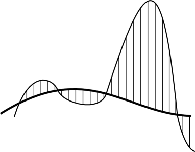
Figure 1: A symbolical connection between solutions of the same metric theory in the geometrical and field-theoretical forms.

Let us discuss some of important points. First, a possibility to use an arbitrary curved background means that any solution of the initial metric theory can be considered as a background. Thus, the background can be flat, curved vacuum, or even curved including background matter, i.e. it can be arbitrary. Second, as was accented, the field and geometrical formulations of the theory have to be equivalent. This means that a solution of the field formulation united together with a background solution have to be transformable into a solution of the geometric formulation (initial metric theory). Symbolically this situation is explained on the figure 1. Let the slightly sloping curve be related to a background and let the oscillating curve mean a solution in the geometrical form, then the difference between them symbolizes the solution in the field-theoretical form. Third, usually it is assumed that a perturbation of a quantity is less than a quantity itself. We do not impose this restriction here. A realization of the requirements (a) - (h) means that the field-theoretical formulation can be thought of as an independent exact field theory. Then, of course, the “amplitude” of an exact solution of the exact theory can be more than “amplitude” of the background (see, e.g., the right side of the figure 1).

At the earlier stage, Einstein was trying to construct a gravitational theory as a field theory in Minkowski space, in the framework of special relativity. However, step by step he had concluded that one needs to operate with curved spacetime only, Minkowski background space had disappeared from the consideration all together. The construction of the field-theoretical formulation in the framework of the geometrical theory is, in a definite sense, the revival of the special relativity view. Moreover, as we remarked above, the field-theoretical formulation really is an independent field theory and can be constructed by independent ways (see below the discussion in subsections 2.1 and 2.2). However, there is no contradiction here. The geometrical and field-theoretical formulations are two different formulations of the same theory with the same physical content. The background spacetime turns out non-observable and has a sense of only an auxiliary structure.

Up to now the Einstein theory retains its position as the most popular theory of gravity, leading in all the applications. Thus, in this paper we pay a significant attention to constructing the field-theoretical formulation for GR which is presented in detail. On the other hand, due to the rising precision of experiments and observables in cosmos and due to the great interest to the brane models, other metric theories generalizing GR become more and more popular and necessary. One of the main properties of the approach presented here is its universality. We use this advantage and develop the field theoretical approach applied to an arbitrary metric theory.

The paper is organized as follows. The next section 2 is devoted to the detail description of the field-theoretical formulation of GR on an arbitrary curved background, which have all the properties of a self-dependent field theory. The essential attention is paid to an invariance with respect to exact gauge transformations. The last do not effect both coordinates and background quantities in the field-theoretical formulation and are connected with the general covariance of GR.

In section 3, we construct conservation laws for perturbations in GR in the framework of the field-theoretical approach. Conserved currents and corresponding superpotentials are presented. As an important instruments we use the canonical Nœther method and the Belinfante symmetrization prescription. The conserved quantities and conservation laws are used for examination of asymptotically flat spacetime at spatial infinity, the closed Friedmann model, the Schwarzschild solution and linear perturbations on FRW backgrounds.

In section 4, we develop the field-theoretical approach to describe perturbations in an arbitrary $D$-dimensional metric theory of gravity on a fixed background. We construct generalized conserved currents and corresponding superpotentials with again the essential use of the Nœther and Belinfante methods. The conserved quantities are tested in the Einstein-Gauss-Bonnet gravity for calculating the mass of the Schwarzschild-anti-de Sitter black hole.

1.4 Notations

Here, we present notations, which will appear more frequently and which are more important. In the text, together with these notations, numerous other notations will be used, they will be outlined currently.

• Greek indexes numerate 4-dimensional spacetime coordinates as well as $D$-dimensional spacetime ones. Usually $x^{0}$ means a time coordinate, whereas small Latin indexes from the middle of alphabet $i,\,j,\,k,\,\ldots$ mean 3-dimensional space coordinates or $(D-1)$-dimensional hyperspace coordinates;

• Large Latin indexes $A,\,B,\,C,\,\ldots$ are used as generalized ones for an arbitrary set of tensor densities, for example, $Q^{A}=\{\sqrt{-g}g^{\mu\nu},\,\phi,\,T_{\alpha\beta}\}$;

• A dynamic metric of a metric theory is $g_{\mu\nu}$ ($g=\det g_{\mu\nu}$);

• Bar means that a quantity “$\overline{Q}^{A}$” is a background one;

• Thus, $\overline{g}_{\mu\nu}$ ($\overline{g}=\det\overline{g}_{\mu\nu}$) is a background metric. Indexes of all the quantities of a perturbed system are raised and lowered by the background metric;

• Many expressions are presented as densities of the weight +1. The reasons are as follows. First, all the Nœther identities, which are explored intensively, are such densities in the initial derivation. Second, conservation laws have to be covariant, however partial derivatives are crucial for application of the Gauss theorem. Divergences of both vector densities (conserved currents) and antisymmetric tensor densities (superpotentials) have this duality property. To accent these expressions we use “hats”, as more economical notations in this situation. Thus, a quantity “$\hat{Q}^{A}$” is such a density, it could be a tensor multiplied by $\sqrt{-g}$ or $\sqrt{-\overline{g}}$ (for example, $\hat{Q}^{\alpha\beta}{}_{\gamma}=\sqrt{-\overline{g}}Q^{\alpha\beta}{}_{\gamma}$), or $\hat{Q}^{A}$ could be be independent on these determinants, a situation will be clarified from the context;

• $\eta_{\mu\nu}$ is a Minkowskian metric in the Lorentzian coordinates; sometimes $\sqrt{-\eta}$ is used explicitly instead of $1$ to stress that a quantity, say $\hat{Q}^{\alpha\beta}{}_{\gamma}=\sqrt{-\eta}Q^{\alpha\beta}{}_{\gamma}$, is a density of the weight $+1$;

• $\hat{l}^{\mu\nu}=\hat{g}^{\mu\nu}-\overline{\hat{g}}^{\mu\nu}=\sqrt{-g}g^{\mu\nu}-\sqrt{-\overline{g}}\,\overline{g}^{\mu\nu}$ is a more important form of the metric perturbations;

• Partial derivatives are denoted by $({}_{,i}),\,({}_{,\alpha}),$ or $\partial_{i},\,\partial_{\alpha},$;

• $D_{\alpha}$ and $\overline{D}_{\alpha}$ are covariant derivatives with respect to $g_{\mu\nu}$ and $\overline{g}_{\mu\nu}$ with the Chistoffel symbols $\Gamma^{\alpha}_{\beta\gamma}$ and $\overline{\Gamma}^{\alpha}_{\beta\gamma}$, respectively;

• $\Delta^{\alpha}_{\beta\gamma}=\Gamma^{\alpha}_{\beta\gamma}-\overline{\Gamma}^{\alpha}_{\beta\gamma}$ is the tensor actively used in the paper;

• $\xi^{\alpha}$ is an arbitrary displacement vector, whereas $\lambda^{\alpha}$ is a Killing vector of a background;

• The Lie derivative is defined as

  $$\pounds_{\xi}Q^{A}=-\xi^{\alpha}\overline{D}_{\alpha}Q^{A}+\left.Q^{A}\right|^{\alpha}_{\beta}\overline{D}_{\alpha}\xi^{\beta}\,,$$

  note the opposite sign to the usual one, $\left.Q^{A}\right|^{\alpha}_{\beta}$ is defined by the transformation properties of $Q^{A}$;

• $\zeta_{\mu\nu}=-{\textstyle{1\over 2}}\pounds_{\xi}\overline{g}_{\mu\nu}$ is the tensor actively used in the paper;

• The Lagrangian derivative is defined as usual:

  $$\frac{\delta{Q^{A}(q^{B},\,q^{B}_{,\alpha},\,q^{B}_{,\alpha\beta},\,\ldots)}}{\delta q^{C}}=\frac{\partial Q^{A}}{\partial q^{C}}-\partial_{\alpha}\left(\frac{\partial Q^{A}}{\partial q^{C}_{,\alpha}}\right)+\partial_{\alpha\beta}\left(\frac{\partial Q^{A}}{\partial q^{C}_{,\alpha\beta}}\right)-\ldots$$

• $R^{\alpha}{}_{\mu\beta\nu}$, $R_{\mu\nu}$, $G_{\mu\nu}$, $T_{\mu\nu}$, $R$ and $\overline{R}^{\alpha}{}_{\mu\beta\nu}$, $\overline{R}_{\mu\nu}$, $\overline{G}_{\mu\nu}$, $\overline{T}_{\mu\nu}$,$\overline{R}$ are the Riemannian, Ricci, Einstein, matter energy-momentum tensors and the curvature scalar for the physical and background spacetimes.

• Usually index “L” means a linearization, for example, $G^{L}_{\mu\nu}$ and $\Phi^{L}_{\mu\nu}$ mean linearized pure gravitational and matter parts of the gravitational field equations;

• The conserved currents are defined in the framework of different approaches as follows. In the case of GR: $\hat{J}^{\mu}_{(c)}$ is defined with the use of the canonical Nœther procedure; $\hat{J}^{\mu}_{(s)}$ is defined with the use of the field-theoretical prescription, based on the symmetrical energy-momentum tensor; $\hat{J}^{\mu}_{(B)}$ is the canonical current corrected with the use of the Belinfante method. The correspondent superpotentials in GR are $\hat{J}^{\mu\nu}_{(c)}$, $\hat{J}^{\mu\nu}_{(s)}$ and $\hat{J}^{\mu\nu}_{(B)}$;

• Analogous currents in superpotentials in an arbitrary $D$-dimensional metric theory are respectively $\hat{\cal I}^{\mu}_{(c)}$, $\hat{\cal I}^{\mu}_{(s)}$, $\hat{\cal I}^{\mu}_{(B)}$ and $\hat{\cal I}^{\mu\nu}_{(c)}$, $\hat{\cal I}^{\mu\nu}_{(s)}$, $\hat{\cal I}^{\mu\nu}_{(B)}$;

• $(\alpha\beta)$, $(ik)$ and $[\alpha\beta]$, [ik] mean symmetrization and antisymmetrization;

• $\kappa$ — the “Einstein” constant both in GR and in an arbitrary metric theory.

2 The exact field-theoretical formulation of GR

2.1 Development of the field approach

The study of perturbations in GR, in fact, was begun by Einstein himself. However, as a separate field, the history of the field-theoretical approach in GR began in 40’s — 50’s of XX century. Perturbed Einstein equations are rewritten as follows. Define the metric perturbations on a flat background in the Lorentzian coordinates as $\hat{l}^{\mu\nu}=\hat{g}^{\mu\nu}-\sqrt{-\eta}\eta^{\mu\nu}$; $l^{\mu\nu}=(\sqrt{-\eta})^{-1}\hat{l}^{\mu\nu}$. The terms linear in metric perturbations are placed on the left hand side of the Einstein equations, whereas all the nonlinear terms are transported to the right hand side, and together with a matter energy-momentum tensor are treated as a total (effective) energy-momentum tensor $t^{(tot)}_{\mu\nu}$. Then Einstein equations are rewritten in the equivalent perturbed form as

$$G^{L}_{\mu\nu}=\kappa t^{(tot)}_{\mu\nu}\,$$ (2.1)

where, raising the indexes by $\eta^{\alpha\beta}$, one has the left hand side in the form:

$$G_{L}^{\mu\nu}\equiv{\textstyle{1\over 2}}(l^{\mu\nu,\alpha}{}_{,\alpha}+\eta^{\mu\nu}l^{\alpha\beta}{}_{,\alpha\beta}-l^{\alpha\mu,\nu}{}_{,\alpha}-l^{\alpha\nu,\mu}{}_{,\alpha})\,.$$ (2.2)

Its divergence identically is equal to zero: $\partial_{\nu}G_{L}^{\mu\nu}\equiv 0$. Then, one obtains directly the differential conservation law

$$\partial_{\nu}t_{(tot)}^{\mu\nu}=0\,.$$ (2.3)

This picture was developed in a form of a Lagrangian based field theory with self-interaction in a fixed background spacetime, where $t^{(tot)}_{\mu\nu}$ is obtained by variation of an action with respect to a background metric. Following the introduction in the Deser work [99], below, we shall present the main steps in this derivation, the corresponding bibliography can also be found in [99]. Assume that a field theory of gravity in a Minkowski space is constructed. By known observable tests (see, e.g., textbook [3]), the most preferable type of the gravitational field is the tensor field, say $l^{\mu\nu}$. The linear (approximate) equations have to have the form $G^{L}_{\mu\nu}=0$ and are defined by the quadratic Lagrangian ${\hat{\cal L}}_{(2)}^{g}$. Keeping a symmetrical energy-momentum tensor of matter fields $\phi^{A}$ as a source of $G^{L}_{\mu\nu}$ one obtains

$$G^{L}_{\mu\nu}(l)=\kappa T_{\mu\nu}(\phi,\eta)\,.$$ (2.4)

Identically $\partial_{\nu}G^{L\nu}_{\mu}\equiv 0$, therefore $\partial_{\nu}T^{\nu}_{\mu}=0$. However, there is a contradiction between the conservation law $\partial_{\nu}T^{\nu}_{\mu}=0$ and equations of motion for interacting fields $\phi^{A}$. How does one avoid this? The right hand side of Eq. (2.4) is to be obtained by variation (conventionally) both with respect to $\eta^{\mu\nu}$ and $l^{\mu\nu}$. Therefore one needs to make an exchange $\left\{\phi^{A},\eta^{\mu\nu}\right\}\rightarrow\left\{\phi^{A},\eta^{\mu\nu}+l^{\mu\nu}\right\}$ both in the matter Lagrangian and in the matter energy-momentum tensor. This just means the universality of gravitational interaction. Next, one has to include the gravitational self-interaction. Therefore one adds the symmetrical energy-momentum tensor of the gravitational field $t^{(2)g}_{\mu\nu}(l)$, corresponding to ${\hat{\cal L}}_{(2)}^{g}$, to the right hand side of (2.4) together with $T_{\mu\nu}(\phi,\eta+l)$. But the equations that include $t^{(2)g}_{\mu\nu}(l)$ can be obtained if a cubic Lagrangian is added, ${\hat{\cal L}}_{(2)}^{g}+{\hat{\cal L}}_{(3)}^{g}$. After this one needs to consider the next level, and so on. In the result, one obtains the final variant of the gravitational equations:

$$G^{L}_{\mu\nu}(l)=\kappa\left[T_{\mu\nu}(\phi,l+\eta)+\sum_{n=2}^{\infty}t^{(n)g}_{\mu\nu}(l)\right]\,.$$ (2.5)

It turns out that the equations (2.5) are exactly the Einstein equations, i.e. equations (2.1). After the identification $\sqrt{-\eta}\eta^{\mu\nu}+\hat{l}^{\mu\nu}\equiv\sqrt{-g}g^{\mu\nu}$ one has only the dynamical metric $g^{\mu\nu}$, whereas the background metric $\eta^{\mu\nu}$ and the field $l^{\mu\nu}$ completely disappear from the consideration.

Deser himself [99], unlike (2.5), has suggested the field formulation of GR without expansions. As dynamical variables he used the two independent tensor fields $l^{\mu\nu}$ and $\Delta^{\alpha}_{\mu\nu}$ of the 1-st order formalism. After variation of the corresponding action he derives the equations in the form:

$$G^{L}_{\mu\nu}(l)=\kappa\left[t^{g}_{\mu\nu}(l,\Delta)+t^{m}_{\mu\nu}\right]\,,$$ (2.6)

instead of (2.5). After identifications $\sqrt{-\eta}\eta^{\mu\nu}+\hat{l}^{\mu\nu}\equiv\sqrt{-g}g^{\mu\nu}$ and $\Delta^{\alpha}_{\mu\nu}\equiv\Gamma^{\alpha}_{\mu\nu}$ the equivalence with the Einstein equations is confirmed, but only in the Palatini form, where $g^{\mu\nu}$ and $\Gamma^{\alpha}_{\mu\nu}$ are used as independent variables.

In the work [100] we have generalized the Deser approach [99]. Instead of the background Minkowski space with the Lorenzian coordinates we consider an arbitrary curved background spacetime with a given metric $\overline{g}_{\mu\nu}$ and given matter fields $\overline{\Phi}^{A}$ satisfying the background Einstein gravitational and matter equations. We also use the 1-st order formalism. The gravitational equations get the generalized form:

$$\hat{G}^{L}_{\mu\nu}(l)+\hat{\Phi}^{L}_{\mu\nu}(l,\phi)=\kappa\left[\hat{t}^{g}_{\mu\nu}(l,\Delta)+\hat{t}^{m}_{\mu\nu}\right]\,$$ (2.7)

where the left hand side is linear in $\hat{l}^{\mu\nu}$ and $\phi^{A}$ and defined later in Eqs. (2.24) - (2.26). The term $\hat{\Phi}^{L}_{\mu\nu}$ appears due to $\overline{\Phi}^{A}$. Equivalence with GR in the ordinary derivation is stated after identifications: $\overline{\hat{g}}^{\mu\nu}+\hat{l}^{\mu\nu}\equiv\hat{g}^{\mu\nu}$, $\overline{\Gamma}^{\alpha}_{\mu\nu}+\Delta^{\alpha}_{\mu\nu}\equiv\Gamma^{\alpha}_{\mu\nu}$ and $\overline{\Phi}^{A}+\phi^{A}\equiv\Phi^{A}$. In the following years we have developed the principles of the work [100] and have used this approach in many applications. Our results are presented in the papers [101] - [121], on the basis of which, in a more part, the present review was written.

Elements of the field approach in gravity are also actively developing nowadays in other approaches. Thus, in [122], a requirement only of the first derivatives of metrical perturbations in the total symmetrical energy-momentum tensor has led to a new field formulation of GR in Minkowski spacetime, which is different from the formulation in [100]. The new total energy-momentum tensor is the source for the non-linear left hand side. On the basis of this new field formulation an interesting variant of the gravitational theory with non-zero masses of gravitons was developed [123]. A comparison and a connection of the works [100, 122, 123] are discussed in [124] in detail. In [125], the work [100] was developed to construct the total energies and angular momenta for $d+1$-dimensional asymptotically anti-de Sitter spacetime. The properties of the field approach [100] appear independently in many concrete problems. For example, in [126, 127] a consideration of linear perturbations on FRW backgrounds leads to the linear approximation of the exact field formulation of GR [100]. In [128], as a development of the field approach, a class of so-called “slightly bimetric” gravitation theories was constructed. In [129, 130], a behaviour of light cones in Minkowski space and effectively curved spacetimes was examined. Then, based on the causality principle, a special criterium was stated. In [131] this criterium was used to show that if spatially flat FRW big bang model is considered as a configuration on a flat background, then the cosmological singularity is banished to past infinity in Minkowski space. The references to earlier works and the theoretical foundation for the field approach can be found in the works [132] - [134]. To the best of our knowledge up to date bibliography related to the field approach in gravity can be found in [128] - [131].

2.2 Various directions in the construction

There are various possibilities to approach the field-theoretical formulation of GR, which are based on different foundations. Here, we shall discuss the well known and important ones. The principle used by Deser [99] could be formulated as follows:

• The source of the linear massless field of spin two (of gravitational field) in Minkowski space is to be the total symmetrical (metric) energy-momentum tensor of all the dynamical fields, including the gravitational field itself.

Using this principle Deser has constructed a corresponding Lagrangian and field equations and energy-momentum tensor following from it. We have generalized the Deser approach on arbitrary curved backgrounds [100]. His principle has been reformulated in a way that the linear left hand side of perturbed gravitational equations has to be of the form in Eq. (2.7), i.e. together with $\hat{G}^{L}_{\mu\nu}$ one has to include the, linear in matter perturbations, part $\hat{\Phi}^{L}_{\mu\nu}$. The analogous principle was suggested for perturbed matter equations.

The next known method was most clearly presented by Grishchuk [134] and shortly can be formulated as:

• A transformation from gravistatic (Newton law) to gravidynamics, i.e. to a relativistic theory of gravitational field (general relativity), equations of which (Einstein equations) describe gravitational waves.

Following this direction, one has to transform the Newton law $\Delta\phi=-4\pi G\rho$ into a special relativity description. To satisfy the relativistic requirement a) the mass density $\rho$ has to be generalized to 10 components of the matter stress-energy tensor $T_{\mu\nu}$; b) the single component $\phi$ should also be replaced by 10 gravitational potentials $l^{\mu\nu}$; c) the Laplace operator should be replaced by the d’Alembert operator; d) the gravitational field has to be nonlinear and, thus, has to be a source for itself. Following this reformations one obtains the generalized equations: ${\textstyle{1\over 2}}l^{~{}~{}~{},\alpha}_{\mu\nu~{}~{},\alpha}=\kappa(t^{g}_{\mu\nu}+T_{\mu\nu})$. They imply that the gauge condition $l^{\mu\nu}_{~{}~{}~{},\nu}=0$ is already chosen. e) To reconstruct the gauge invariance properties it is necessary to add to the left hand side the terms ${\textstyle{1\over 2}}\left(\eta_{\mu\nu}l^{\alpha\beta}_{~{}~{}~{},\alpha,\beta}-l^{\alpha}_{~{}\mu,\nu,\alpha}-l^{\alpha}_{~{}\nu,\mu,\alpha}\right)$. As a result, one obtains Eq. (2.1), which is just the Einstein equations.

The field formulation of GR can be also constructed based on the gauge properties (see our work [107]). This direction is analogous to the method in the gauge theories of the Yang-Mills type, which are constructed by localizing parameters of a gauge group. However, unlike usual, we postulate a non-standard way of localization, namely:

• A “localization” of Killing vectors of the background spacetime.

This assumes the existence of a fixed background spacetime with symmetries presented by a Killing vector field $\lambda^{\alpha}$, in which initial dynamic fields $\phi^{A}$ are propagated. It is noted that an action for the initial fields is invariant, up to a surface term, under the transformation $\phi^{A}\rightarrow\pounds_{\lambda}\phi^{A}$. Next, the Killing vector is changed for an arbitrary vector $\xi^{\alpha}$, that is localized. Then the invariance is destroyed. To restore it the compensating (gauge) field has to be included. In doing so the coordinates and the background metric do not change. The requirements to have the gauge field as an universal field and to have the simplest sought-for action for the free gauge field lead just to the field formulation of GR, developed in [100].

As a rule, a fixed background spacetime, in which perturbations are studied, is determined by the problem under consideration (see subsections 1.1 and 1.2 in Introduction). Thus the background could be assumed as a known solution to the Einstein equations. Then one has to study the perturbed (with respect to this background) Einstein equations. As already was noted above, this picture can be developed as a Lagrangian based field theory, where the first step is:

• The decomposition of dynamical variables of GR into background variables and dynamic perturbations.

This method is evident in itself and has the explicit connection with the ordinary geometrical formulation of GR. Namely this method is easily adopted for constructing the field-theoretical formulation in the framework of an arbitrary metric theory. In the next subsections, basing on the works [100, 103, 104], we present it in detail. However, although the construction was developed for both in the 1-st and in the 2-nd order formalisms, here, we use the 2-nd order formalism only since it is more convenient and suitable. To the best of our knowledge, Barnebey [135] was the first who suggested to use the 2-nd order formalism for an exact (without expansions) description of perturbations in GR.

2.3 A dynamical Lagrangian

Let us consider the Einstein theory and write out its action

$$S={1\over c}\int d^{4}x\hat{\cal L}^{E}\equiv-{1\over{2\kappa c}}\int d^{4}x\hat{R}(g_{\mu\nu})+{1\over c}\int d^{4}x\hat{\cal L}^{M}(\Phi^{A},~{}g_{\mu\nu})\,,$$ (2.8)

$\hat{\cal L}^{M}$ depends on $\Phi^{A}$ and their derivatives up to a finite order. Then, the gravitational and matter equations corresponding to the Lagrangain (2.8) are

$${{\delta{{\hat{\cal L}}}^{E}}\over{\delta\hat{g}^{\mu\nu}}}=-{1\over{2\kappa}}{{\delta\hat{R}}\over{\delta\hat{g}^{\mu\nu}}}+{{\delta{{\hat{\cal L}}}^{M}}\over{\delta\hat{g}^{\mu\nu}}} = 0\,,$$ (2.9)

$${{\delta{{\hat{\cal L}}}^{E}}\over{\delta\Phi^{A}}}={{\delta{\hat{\cal L}}^{M}}\over{\delta\Phi^{A}}} = 0\,.$$ (2.10)

The form of Eq. (2.9) corresponds to the form of the Einstein equations

$$R_{\mu\nu}-\kappa\left(T_{\mu\nu}-{\textstyle{1\over 2}}g_{\mu\nu}T^{\alpha}_{\alpha}\right)=0\,,$$ (2.11)

whereas a more customary form is

$$\sqrt{-g}\left({G}_{\mu\nu}-\kappa{T}_{\mu\nu}\right)\equiv{\hat{G}}_{\mu\nu}-\kappa{\hat{T}}_{\mu\nu}=0\,,$$ (2.12)

which is obtained by variation with respect to $g^{\mu\nu}$.

Next, let us define the metric and matter perturbations with the use of the decompositions:

$$\hat{g}^{\mu\nu}\equiv\overline{\hat{g}}^{\mu\nu}+\hat{l}^{\mu\nu}\,,$$ (2.13)

$$\Phi^{A}\equiv\overline{\Phi}^{A}+\phi^{A}\,.$$ (2.14)

It is assumed that the background quantities $\overline{\hat{g}}^{\mu\nu}$ and $\overline{\Phi}^{A}$ are known and satisfy the background (given) system, which is defined as follows. Its action is

$$\overline{S}={1\over c}\int{d^{4}x\overline{{{\hat{\cal L}}}^{E}}}\equiv-{1\over{2\kappa c}}\int{d^{4}x\overline{\hat{R}}}+{1\over c}\int{d^{4}x\overline{{{\hat{\cal L}}}^{M}}}\,.$$ (2.15)

The corresponding to the Lagrangian in (2.15) background gravitational and matter equations have the form of the barred equations (2.9) and (2.10):

$$-{1\over{2\kappa}}{{\delta\overline{\hat{R}}}\over{\delta\overline{\hat{g}}^{\mu\nu}}}+{{\delta\overline{{{\hat{\cal L}}}^{M}}}\over{\delta\overline{\hat{g}}^{\mu\nu}}} = 0\,,$$ (2.16)

$${{\delta\overline{{{\hat{\cal L}}}^{M}}}\over{\delta\overline{\Phi}^{A}}} = 0\,.$$ (2.17)

Frequently we use a Ricci-flat background with the background equations

$$\overline{\hat{G}}_{\mu\nu}=\overline{\hat{R}}_{\mu\nu}=0.$$ (2.18)

Now let us classify the perturbations $\hat{l}^{\mu\nu}$ and $\phi^{A}$ as independent dynamic variables, which present a field configuration on the background of the system (2.16) and (2.17). To describe this dynamical configuration we construct a corresponding Lagrangian called as a dynamical one [104]. After substituting the decompositions (2.13) and (2.14) into the Lagrangian ${\hat{\cal L}}^{E}$ of the action (2.8) and subtracting zero’s and linear in $\hat{l}^{\mu\nu}$ and $\phi^{A}$ terms of the functional expansion of the Lagrangian ${\hat{\cal L}}^{E}$ one has

$${{\hat{\cal L}}}^{dyn}={{\hat{\cal L}}}^{E}(\overline{g}+l,\,\overline{\Phi}+\phi)-\hat{l}^{\mu\nu}{{\delta\overline{{\hat{\cal L}}^{E}}}\over{\delta\overline{\hat{g}}^{\mu\nu}}}-\phi^{A}{{\delta\overline{{\hat{\cal L}}^{E}}}\over{\delta\overline{\Phi}^{A}}}-\overline{{\hat{\cal L}}^{E}}-{1\over{2\kappa}}\partial_{\alpha}\hat{k}^{\alpha}=-{1\over{2\kappa}}{\hat{\cal L}}^{g}+{\hat{\cal L}}^{m}\,.$$ (2.19)

As is seen, zero’s order term is the background Lagrangian, whereas the linear term is proportional to the left hand sides of the background equations (2.16) and (2.17).

In Eq. (2.19) a vector density $\hat{k}^{\alpha}$ is not concreted. However, consider $\hat{k}^{\alpha}$ defined as

$$\hat{k}^{\alpha}\equiv\hat{g}^{\alpha\nu}\Delta^{\mu}_{\mu\nu}-\hat{g}^{\mu\nu}\Delta^{\alpha}_{\mu\nu}\,$$ (2.20)

with $\Delta^{\rho}_{\mu\nu}$ presented as the perturbations of the Cristoffel symbols

$$\Delta^{\alpha}_{\mu\nu}\equiv\Gamma^{\alpha}_{\mu\nu}-\overline{\Gamma}^{\alpha}_{\mu\nu}={\textstyle{1\over 2}}g^{\alpha\rho}\left(\overline{D}_{\mu}g_{\rho\nu}+\overline{D}_{\nu}g_{\rho\mu}-\overline{D}_{\rho}g_{\mu\nu}\right)\,,$$ (2.21)

and depending on $\hat{l}^{\mu\nu}$ through the decomposition (2.13). Then a pure gravitational part in the Lagrangian (2.19) is presented in the form:

$${\hat{\cal L}}^{g} = \hat{R}(\overline{\hat{g}}^{\mu\nu}+\hat{l}^{\mu\nu})-\hat{l}^{\mu\nu}\overline{R}_{\mu\nu}-\overline{\hat{g}}^{\mu\nu}\overline{R}_{\mu\nu}+\partial_{\mu}\hat{k}^{\mu}\,$$ (2.22)

$$= -(\Delta^{\rho}_{\mu\nu}-\Delta^{\sigma}_{\mu\sigma}\delta^{\rho}_{\nu})\overline{D}_{\rho}\hat{l}^{\mu\nu}+(\overline{{\hat{g}}}^{\mu\nu}+\hat{l}^{\mu\nu})\left(\Delta^{\rho}_{\mu\nu}\Delta^{\sigma}_{\rho\sigma}-\Delta^{\rho}_{\mu\sigma}\Delta^{\sigma}_{\rho\nu}\right)\,.$$

It depends only on the first derivatives of the gravitational variables $\hat{l}^{\mu\nu}$. In the case of a flat background the Lagrangian (2.22) transfers to the covariant Lagrangian suggested by Rosen [136], which has been rediscovered in [137] and [101]. The matter part of (2.19) is

$${\hat{\cal L}}^{m}={{\hat{\cal L}}}^{M}\left(\overline{g}+l,\,\overline{\Phi}+\phi\right)-\hat{l}^{\mu\nu}{{\delta\overline{{\hat{\cal L}}^{M}}}\over{\delta\overline{\hat{g}}^{\mu\nu}}}-\phi^{A}{{\delta\overline{{\hat{\cal L}}^{M}}}\over{\delta\overline{\Phi}^{A}}}-\overline{{\hat{\cal L}}^{M}}\,.$$

2.4 The Einstein equations in the field formulation

The variation of the action with the Lagrangian (2.19) with respect to $\hat{l}^{\alpha\beta}$ and the contraction with $\sqrt{-\overline{g}}(\delta^{\alpha}_{\mu}\delta^{\beta}_{\nu}-{\textstyle{1\over 2}}\overline{g}_{\mu\nu}\overline{g}^{\alpha\beta})$ give the field equations in the form:

$$\hat{G}^{L}_{\mu\nu}+\hat{\Phi}^{L}_{\mu\nu}=\kappa\left({\hat{t}}^{g}_{\mu\nu}+{\hat{t}}^{m}_{\mu\nu}\right)\equiv\kappa{\hat{t}}^{(tot)}_{\mu\nu}\,.$$ (2.23)

They coincide with the form (2.7), only now in the 2-nd order formalism. The left hand side of Eq. (2.23) is linear in $\hat{l}^{\mu\nu}$ and $\phi^{A}$. It consists of the pure gravitational part

$$\hat{G}^{L}_{\mu\nu}(\hat{l})\equiv{\delta\over{\delta\overline{g}^{\mu\nu}}}\hat{l}^{\rho\sigma}{{\delta\overline{\hat{R}}}\over{\delta\overline{\hat{g}}^{\rho\sigma}}}$$ (2.24)

$$\equiv {\textstyle{1\over 2}}\left({\overline{D}_{\rho}}{\overline{D}^{\rho}}\hat{l}_{\mu\nu}+{\overline{g}_{\mu\nu}}{\overline{D}_{\rho}}{\overline{D}_{\sigma}}\hat{l}^{\rho\sigma}-{\overline{D}_{\rho}}{\overline{D}_{\nu}}\hat{l}_{\mu}^{~{}\rho}-{\overline{D}_{\rho}}{\overline{D}_{\mu}}\hat{l}_{\nu}^{~{}\rho}\right),$$ (2.25)

which is the covariantized expression (2.2), and of the matter part

$$\hat{\Phi}^{L}_{\mu\nu}(\hat{l},\phi)\equiv-2\kappa{\delta\over{\delta\overline{g}^{\mu\nu}}}\left(\hat{l}^{\rho\sigma}{{\delta\overline{{\hat{\cal L}}^{M}}}\over{\delta\overline{\hat{g}}^{\rho\sigma}}}+\phi^{A}{{\delta{\overline{{\hat{\cal L}}^{M}}}}\over{\delta{\overline{\Phi}^{A}}}}\right)\,.$$ (2.26)

It disappears for Ricci-flat backgrounds (2.18), and then Eq. (2.23) acquires the form of Eq. (2.1). The right hand side of Eq. (2.23) is the symmetrical energy-momentum tensor density

$${\hat{t}}^{(tot)}_{\mu\nu}\equiv 2{{\delta{{\hat{\cal L}}}^{dyn}}\over{\delta\overline{g}^{\mu\nu}}}\equiv 2{{\delta}\over{\delta\overline{g}^{\mu\nu}}}\left(-{1\over{2\kappa}}{\hat{\cal L}}^{g}+{\hat{\cal L}}^{m}\right)\equiv{\hat{t}}^{g}_{\mu\nu}+{\hat{t}}^{m}_{\mu\nu}.$$ (2.27)

The explicit form of the gravitational part is

$${\hat{t}}^{g}_{\mu\nu}={1\over\kappa}\left[\sqrt{-\overline{g}}\left(-\delta^{\rho}_{\mu}\delta^{\sigma}_{\nu}+{\textstyle{1\over 2}}\overline{g}_{\mu\nu}\overline{g}^{\rho\sigma}\right)\left(\Delta^{\alpha}_{\rho\sigma}\Delta^{\beta}_{\alpha\beta}-\Delta^{\alpha}_{\rho\beta}\Delta^{\beta}_{\alpha\sigma}\right)+\overline{D}_{\tau}\hat{Q}^{\tau}_{\mu\nu}\right]\,;$$ (2.28)

$$2\hat{Q}^{\tau}_{\mu\nu} \equiv -\overline{g}_{\mu\nu}\hat{l}^{\alpha\beta}\Delta^{\tau}_{\alpha\beta}+\hat{l}_{\mu\nu}\Delta^{\tau}_{\alpha\beta}\overline{g}^{\alpha\beta}-\hat{l}^{\tau}_{\mu}\Delta^{\alpha}_{\nu\alpha}-\hat{l}^{\tau}_{\nu}\Delta^{\alpha}_{\mu\alpha}+\hat{l}^{\beta\tau}\left(\Delta^{\alpha}_{\mu\beta}\overline{g}_{\alpha\nu}+\Delta^{\alpha}_{\nu\beta}\overline{g}_{\alpha\mu}\right)$$ (2.29)

$$+ \hat{l}^{\beta}_{\mu}\left(\Delta^{\tau}_{\nu\beta}-\Delta^{\alpha}_{\beta\rho}\overline{g}^{\rho\tau}\overline{g}_{\alpha\nu}\right)+\hat{l}^{\beta}_{\nu}\left(\Delta^{\tau}_{\mu\beta}-\Delta^{\alpha}_{\beta\rho}\overline{g}^{\rho\tau}\overline{g}_{\alpha\mu}\right)\,.$$

The matter part is expressed through the usual matter energy-momentum tensor density $\hat{T}_{\mu\nu}$ of the Einstein theory as

$$\hat{t}^{m}_{\mu\nu} = \hat{T}_{\mu\nu}-{{\textstyle{1\over 2}}}g_{\mu\nu}\hat{T}_{\alpha\beta}g^{\alpha\beta}-{{\textstyle{1\over 2}}}\overline{g}_{\mu\nu}\overline{g}^{\alpha\beta}\left(\hat{T}_{\alpha\beta}-{{\textstyle{1\over 2}}}g_{\alpha\beta}\hat{T}_{\pi\rho}g^{\pi\rho}\right)$$ (2.30)

$$-\,2{\delta\over{\delta\overline{g}^{\mu\nu}}}\left(\hat{l}^{\rho\sigma}{{\delta\overline{{\hat{\cal L}}^{M}}}\over{\delta\overline{\hat{g}}^{\rho\sigma}}}+\phi^{A}{{\delta{\overline{{\hat{\cal L}}^{M}}}}\over{\delta{\overline{\Phi}^{A}}}}\right)-\overline{\hat{T}}_{\mu\nu}\,.$$

Taking into account the definitions (2.26), (2.27) and (2.30) in the field equations (2.23) one can rewrite them in the form:

$$\hat{G}^{L}_{\mu\nu}=\kappa\left({\hat{t}}^{g}_{\mu\nu}+\delta{\hat{t}}^{M}_{\mu\nu}\right)=\kappa\hat{t}^{(eff)}_{\mu\nu}\,;$$ (2.31)

$$\delta{\hat{t}}^{M}_{\mu\nu}\equiv{\hat{t}}^{M}_{\mu\nu}-\overline{\hat{t}^{M}}_{\mu\nu}=\hat{T}_{\mu\nu}-{\textstyle{1\over 2}}g_{\mu\nu}g^{\rho\sigma}\hat{T}_{\rho\sigma}-{\textstyle{1\over 2}}\overline{g}_{\mu\nu}\overline{g}^{\rho\sigma}\left(\hat{T}_{\rho\sigma}-{\textstyle{1\over 2}}g_{\rho\sigma}g^{\lambda\tau}\hat{T}_{\lambda\tau}\right)-\overline{\hat{T}}_{\mu\nu}\,.$$ (2.32)

The equation (2.31) has the form of Eq. (2.1) even on arbitrary backgrounds. The price is that the effective source $\hat{t}^{(eff)}_{\mu\nu}$, including the matter part as $\delta{\hat{t}}^{M}_{\mu\nu}$, does not follow from the Lagrangian (2.19) directly. However, this matter part could be classified as a perturbation of

$${\hat{t}}^{M}_{\mu\nu}\equiv\frac{\delta{\hat{\cal L}}^{M}\left(\overline{\Phi}^{A}+\phi^{A};~{}\overline{\hat{g}}^{\mu\nu}+\hat{l}^{\mu\nu}\right)}{\delta\overline{g}^{\mu\nu}}\,.$$ (2.33)

Return to the equations (2.23) in the whole. Transfer the energy-momentum tensor density to the left hand side and use the definitions (2.24), (2.26) and (2.27) with (2.19):

$$\hat{G}^{L}_{\mu\nu}+\hat{\Phi}^{L}_{\mu\nu}-\kappa{\hat{t}}^{(tot)}_{\mu\nu}\equiv$$

$$-2\kappa{{\partial\overline{\hat{g}}^{\rho\sigma}}\over{\partial\overline{g}^{\mu\nu}}}{{\delta}\over{\delta{\hat{l}^{\rho\sigma}}}}\left[-{1\over{2\kappa}}\hat{R}\left(\overline{\hat{g}}^{\alpha\beta}+\hat{l}^{\alpha\beta}\right)+{{\hat{\cal L}}}^{M}\left(\overline{\Phi}^{A}+\phi^{A};~{}\overline{\hat{g}}^{\mu\nu}+\hat{l}^{\mu\nu}\right)\right]$$

$$+~{}2\kappa{{\delta}\over{\delta\overline{g}^{\mu\nu}}}\left(-{1\over{2\kappa}}\overline{\hat{R}}+\overline{{\hat{\cal L}}}^{M}\right)=0\,.$$ (2.34)

Because the second line contains the operator of the background Einstein equations in (2.16) one can assert that Eq. (2.23) is equivalent to the Einstein equations (2.9).

By the same way the perturbed matter equations are constructed. They have the form:

$$\Phi^{L}_{A}=t^{m}_{A}$$ (2.35)

where

$$\Phi^{L}_{A}(\hat{l},\phi) \equiv -{\delta\over{\delta\overline{\Phi}^{A}}}\left(\hat{l}^{\rho\sigma}{{\delta\overline{{\hat{\cal L}}^{M}}}\over{\delta\overline{\hat{g}}^{\rho\sigma}}}+\phi^{B}{{\delta{\overline{{\hat{\cal L}}^{M}}}}\over{\delta{\overline{\Phi}^{B}}}}\right)\,,$$ (2.36)

$$t^{m}_{A} \equiv {{\delta{\hat{\cal L}}^{m}}\over{\delta\overline{\Phi}^{A}}}\,.$$ (2.37)

2.5 Expansions

The methods of the exact field-theoretical formulation give a possibility to construct an approximate scheme easily and in clear expressions up to an arbitrary order in perturbations. Let us show this. Assuming enough smooth functions, expand the Lagrangian ${\hat{\cal L}}^{E}(\overline{g}+l,\,\overline{\Phi}+\phi)$ as

$${{\hat{\cal L}}}^{E} = \overline{{\hat{\cal L}}^{E}}+\hat{l}^{\rho\sigma}{{\delta\overline{{\hat{\cal L}}^{E}}}\over{\delta\overline{\hat{g}}^{\rho\sigma}}}+\phi^{B}{{\delta{\overline{{\hat{\cal L}}^{E}}}}\over{\delta{\overline{\Phi}^{B}}}}+$$ (2.38)

$$+ \frac{1}{2!}\hat{l}^{\alpha\beta}{{\delta}\over{\delta\overline{\hat{g}}^{\alpha\beta}}}\hat{l}^{\rho\sigma}{{\delta{{{\overline{{\hat{\cal L}}^{E}}}}}}\over{\delta\overline{\hat{g}}^{\rho\sigma}}}+\hat{l}^{\rho\sigma}{{\delta}\over{\delta\overline{\hat{g}}^{\rho\sigma}}}\phi^{A}{{\delta{{\overline{{\hat{\cal L}}^{E}}}}}\over{\delta\overline{\Phi}^{A}}}+\frac{1}{2!}\phi^{B}{{\delta}\over{\delta\overline{\Phi}^{B}}}\phi^{A}{{\delta{{\overline{{\hat{\cal L}}^{E}}}}}\over{\delta\overline{\Phi}^{A}}}+$$

$$+ \frac{1}{3!}\hat{l}^{\mu\nu}{{\delta}\over{\delta\overline{\hat{g}}^{\mu\nu}}}\hat{l}^{\alpha\beta}{{\delta}\over{\delta\overline{\hat{g}}^{\alpha\beta}}}\hat{l}^{\rho\sigma}{{\delta{{\overline{{\hat{\cal L}}^{E}}}}}\over{\delta\overline{\hat{g}}^{\rho\sigma}}}+\ldots+div\,.$$

Then the dynamical Lagrangian (2.19) acquires the form:

$${{\hat{\cal L}}}^{dyn}=\frac{1}{2!}\hat{l}^{\alpha\beta}{{\delta}\over{\delta\overline{\hat{g}}^{\alpha\beta}}}\hat{l}^{\rho\sigma}{{\delta{{{\overline{{\hat{\cal L}}^{E}}}}}}\over{\delta\overline{\hat{g}}^{\rho\sigma}}}+\hat{l}^{\rho\sigma}{{\delta}\over{\delta\overline{\hat{g}}^{\rho\sigma}}}\phi^{A}{{\delta{{\overline{{\hat{\cal L}}^{E}}}}}\over{\delta\overline{\Phi}^{A}}}+\frac{1}{2!}\phi^{B}{{\delta}\over{\delta\overline{\Phi}^{B}}}\phi^{A}{{\delta{{\overline{{\hat{\cal L}}^{E}}}}}\over{\delta\overline{\Phi}^{A}}}+\ldots+div\,.$$ (2.39)

First, note that a divergence in (2.39) is not so important because divergences vanish under the Lagrange derivative. Second, now we can explain why in the linear terms of the Lagrangian (2.19) the background equations are not taken into account before variation. Indeed, the Lagrangian ${\hat{\cal L}}^{E}(\overline{g}+l,\,\overline{\Phi}+\phi)$ in (2.19) contains the same linear terms with only the opposite sign not explicitly (the formula (2.38) shows this). Therefore, in fact, these linear terms are compensated, and the real lowest order in the expansion of ${\hat{\cal L}}^{dyn}$ is a quadratic one (2.39). In this relation, recall that in the usual geometrical description of GR the attempt to define the energy-momentum tensor through $\delta{\hat{\cal L}}^{E}/\delta g^{\mu\nu}$ leads to zero on the solutions of the Einstein equations. In contrast, ${\hat{t}}^{(tot)}_{\mu\nu}$ in (2.27) does not vanish on the field equations. The reason is just in the presence in the Lagrangian (2.19) of these linear terms.

Third, under necessary assumptions the series (2.39) can be interrupted at a corresponding order. Thus the approximate Lagrangian for the perturbed system can be obtained. Its variation gives both approximate field equations and energy-momentum tensor. For example, the quadratic approximation of (2.39) gives a possibility a) to construct the linear equations

$$-\frac{1}{2\kappa}\left(\hat{G}^{L}_{\mu\nu}(\hat{l},\phi)+\hat{\Phi}^{L}_{\mu\nu}(\hat{l},\phi)\right) \equiv {\delta\over{\delta\overline{g}^{\mu\nu}}}\left(\hat{l}^{\rho\sigma}{{\delta\overline{{\hat{\cal L}}^{E}}}\over{\delta\overline{\hat{g}}^{\rho\sigma}}}+\phi^{B}{{\delta{\overline{{\hat{\cal L}}^{E}}}}\over{\delta{\overline{\Phi}^{B}}}}\right)=0\,,$$ (2.40)

$$-\Phi^{L}_{A}(\hat{l},\phi) \equiv {\delta\over{\delta\overline{\Phi}^{A}}}\left(\hat{l}^{\rho\sigma}{{\delta\overline{{\hat{\cal L}}^{E}}}\over{\delta\overline{\hat{g}}^{\rho\sigma}}}+\phi^{B}{{\delta{\overline{{\hat{\cal L}}^{E}}}}\over{\delta{\overline{\Phi}^{B}}}}\right)=0\,,$$ (2.41)

b) to construct the quadratic energy-momentum tensor:

$$t^{(tot)}_{\mu\nu}=\frac{2}{\sqrt{\overline{g}}}\frac{\delta}{\delta\overline{g}^{\mu\nu}}\left(\frac{1}{2!}\hat{l}^{\alpha\beta}{{\delta}\over{\delta\overline{\hat{g}}^{\alpha\beta}}}\hat{l}^{\rho\sigma}{{\delta{{{\overline{{\hat{\cal L}}^{E}}}}}}\over{\delta\overline{\hat{g}}^{\rho\sigma}}}+\hat{l}^{\rho\sigma}{{\delta}\over{\delta\overline{\hat{g}}^{\rho\sigma}}}\phi^{A}{{\delta{{\overline{{\hat{\cal L}}^{E}}}}}\over{\delta\overline{\Phi}^{A}}}+\frac{1}{2!}\phi^{B}{{\delta}\over{\delta\overline{\Phi}^{B}}}\phi^{A}{{\delta{{\overline{{\hat{\cal L}}^{E}}}}}\over{\delta\overline{\Phi}^{A}}}\right)\,.$$ (2.42)

The cubic approximation of (2.39) gives a possibility a) to construct the field equations including quadratic terms (which are related to the energy-momentum tensor), and b) to construct the energy-momentum tensor, including quadratic and cubic parts, etc.

Fourth, the expansions, like (2.38) - (2.42), are used in quantum field theories [4] and called as functional expansions. As is seen, in the framework of the classic theory the functional expansions (2.39) - (2.41) give, in fact, the algorithm for constructing the approximate systems, thus an each order can be obtained automatically.

2.6 Gauge transformations and their properties

The important property of the field formulation is the gauge invariance. Usually gauge transformations in GR and other metric theories are connected with mapping a spacetime onto itself that is connected with differentiable coordinate transformations

$${x^{\prime}}^{\alpha}=f^{\alpha}(x^{\beta})\,.$$ (2.43)

These transformations can be connected with the smooth vector field $\xi^{\alpha}$:

$${x^{\prime}}^{\alpha}=x^{\alpha}+\xi^{\alpha}(x)+{1\over{2!}}~{}\xi^{\beta}\xi^{\alpha}_{~{}~{},\beta}+{1\over{3!}}~{}\xi^{\pi}(\xi^{\beta}\xi^{\alpha}_{~{}~{},\beta})_{,\pi}+{...}\,.$$ (2.44)

To map the spacetime onto itself one has to follow the standard way [138] - [140]. After the coordinate transformations (2.43) (or (2.44)) the metric density, for example, is transformed as ${\hat{g}}^{\mu\nu}(x)\rightarrow{\hat{g}}^{\prime\mu\nu}(x^{\prime})$. Then return to the points with quantities $x$ within a new frame $\left\{x^{\prime}\right\}$. After that one has to compare geometrical objects of the initial spacetime and of the mapped spacetime in the points with quantities $x$. The comparison can be carried out both without $\xi^{\alpha}$ in the terms of (2.43) and with $\xi^{\alpha}$ included in (2.44):

$${\hat{g}}^{\prime\mu\nu}(x) = \hat{g}^{\mu\nu}(x)+\delta_{f}\hat{g}^{\mu\nu}=\hat{g}^{\mu\nu}(x)+\sum^{\infty}_{k=1}{1\over{k!}}~{}\hbox{$\pounds$}_{\xi}^{k}{\hat{g}^{\mu\nu}}(x)\,,$$ (2.45)

$${\Phi}^{\prime A}(x) = \Phi^{A}(x)+\delta_{f}\Phi^{A}(x)=\Phi^{A}(x)+\sum^{\infty}_{k=1}{1\over{k!}}~{}\hbox{$\pounds$}_{\xi}^{k}{\Phi^{A}}(x)\,.$$ (2.46)

The next property is very useful. Assume that geometrical objects $\Psi^{B}$ are differentiable functions of other geometrical objects $\psi^{A}$ and their derivatives, but are not explicit functions of coordinates. Then it is clear that a simple substitution gives $\Psi^{B}(\psi^{\prime A})=\Psi^{\prime B}$, and one has

$$\Psi^{B}(\psi^{\prime A}(x))=\Psi^{B}(\psi^{A}(x))+\delta_{f}\Psi^{B}=\Psi^{B}(\psi^{A}(x))+\sum^{\infty}_{k=1}{1\over k!}{\pounds_{\xi}}^{k}\Psi^{B}\,.$$ (2.47)

Now let us define the gauge transformations for the dynamical variables in the framework of the field formulation of GR:

$${\hat{l}}^{\prime\mu\nu} = \hat{l}^{\mu\nu}+\delta_{f}\left(\overline{\hat{g}}^{\mu\nu}+\hat{l}^{\mu\nu}\right)=\hat{l}^{\mu\nu}+\sum^{\infty}_{k=1}{1\over{k!}}~{}\hbox{$\pounds$}_{\xi}^{k}\left(\overline{\hat{g}}^{\mu\nu}+\hat{l}^{\mu\nu}\right),$$ (2.48)

$${\phi}^{\prime A} = \phi^{A}+\delta_{f}\left(\overline{\Phi}^{A}+\phi^{A}\right)=\phi^{A}+\sum^{\infty}_{k=1}{1\over{k!}}~{}\hbox{$\pounds$}_{\xi}^{k}\left(\overline{\Phi}^{A}+\phi^{A}\right).$$ (2.49)

The assumptions above, in fact, state that the operators $\delta_{f}$ and $\sum^{\infty}_{k=1}{\textstyle{1\over{k!}}}~{}\hbox{$\pounds$}_{\xi}^{k}$ are equivalent. However, the operator $\delta_{f}$ could present a wider class of transformations, which cannot be expressed through infinite series. We conserve a possibility to consider such transformations, however more frequently we will use the sums, keeping in mind that they can be changed by $\delta_{f}$ also.

Now, let us substitute (2.48) and (2.49) into the dynamical Lagrangian (2.19). One finds that this substitution into ${{\hat{\cal L}}}^{E}(\overline{\hat{g}}+\hat{l},\overline{\Phi}+\phi)$ just permits to use the property (2.47). Then finally one obtains

$${{\hat{\cal L}}}^{\prime dyn} = {{\hat{\cal L}}}^{dyn}+\sum^{\infty}_{k=1}{1\over k!}{\pounds_{\xi}}^{k}{{\hat{\cal L}}}^{E}(\overline{\hat{g}}+\hat{l},\overline{\Phi}+\phi)-{1\over{2\kappa}}\partial_{\alpha}\left(\hat{k}^{\prime\alpha}-\hat{k}^{\alpha}\right)$$ (2.50)

$$-\left(\hat{l}^{\prime\mu\nu}-\hat{l}^{\mu\nu}\right){{\delta{\overline{{\hat{\cal L}}^{E}}}}\over{\delta\overline{\hat{g}}^{\mu\nu}}}-\left(\phi^{\prime A}-\phi^{A}\right){{\delta{\overline{{\hat{\cal L}}^{M}}}}\over{\delta\overline{\Phi}^{A}}}\,.$$

Because ${{\hat{\cal L}}}^{E}$ is the scalar density of the weight $+1$ all the terms under the sum in (2.50) are divergences. Thus ${{\hat{\cal L}}}^{dyn}$ is gauge invariant up to a divergence if the background equations (2.16) and (2.17) hold.

Considering the gauge invariance properties of the field equations we use their form (2.34). The substitution of (2.48) and (2.49) with the use of the property (2.47) gives

$$\left[\hat{G}^{L}_{\mu\nu}+\hat{\Phi}^{L}_{\mu\nu}-\kappa{\hat{t}}^{(tot)}_{\mu\nu}\right]^{\prime}=\left[\hat{G}^{L}_{\mu\nu}+\hat{\Phi}^{L}_{\mu\nu}-\kappa{\hat{t}}^{(tot)}_{\mu\nu}\right]$$ (2.51)

$$+ {{\partial\overline{\hat{g}}^{\rho\sigma}}\over{\partial\overline{g}^{\mu\nu}}}\sum^{\infty}_{k=1}{1\over k!}{\pounds_{\xi}}^{k}\left[{{\partial\overline{g}^{\delta\pi}}\over{\partial\overline{\hat{g}}^{\rho\sigma}}}\left(\hat{G}^{L}_{\delta\pi}+\hat{\Phi}^{L}_{\delta\pi}-\kappa{\hat{t}}^{(tot)}_{\delta\pi}\right)-2\kappa{{\delta{\overline{{\hat{\cal L}}^{E}}}}\over{\delta\overline{\hat{g}}^{\rho\sigma}}}\right]\,.$$

Thus the field equations are gauge invariant on solutions of themselves and with using the background equations (2.16) and (2.17). Analogous transformations could be presented for the matter equations (2.35).

Concerning the energy-momentum tensor, it is not gauge invariant. Even on the dynamical equations, as it follows from (2.51), under the transformations (2.48) and (2.49) one has

$$\kappa{{\hat{t}}}^{\prime(tot)}_{\mu\nu}=\kappa{\hat{t}}^{(tot)}_{\mu\nu}+\hat{G}^{L}_{\mu\nu}(l^{\prime}-l)+\hat{\Phi}^{L}_{\mu\nu}(l^{\prime}-l;\,\phi^{\prime}-\phi)\,.$$ (2.52)

The mathematical reason is that the background equations in the Lagrangian (2.50) cannot be taken into account before variation. In the case of the Ricci-flat backgrounds (2.18) one has $\hat{\Phi}^{L}_{\mu\nu}=0$, therefore the energy-momentum ${\hat{t}}^{(tot)}_{\mu\nu}$ is gauge invariant up to $\hat{G}^{L}_{\mu\nu}$ — covariant divergence (see (2.25)). Let us turn also to the equivalent form (2.31) of the field equations with the effective source ${\hat{t}}^{(eff)}_{\mu\nu}$. For the operator of the field equations $\hat{G}^{L}_{\mu\nu}-\kappa{\hat{t}}^{(eff)}_{\mu\nu}$ the form of the transformations (2.51) can be used without changing. Then on the field equations one has

$$\kappa{{\hat{t}}}^{\prime(eff)}_{\mu\nu}=\kappa{\hat{t}}^{(eff)}_{\mu\nu}+\hat{G}^{L}_{\mu\nu}(l^{\prime}-l)\,,$$ (2.53)

i.e. for all the kinds of backgrounds ${\hat{t}}^{(eff)}_{\mu\nu}$ is gauge invariant up to a covariant divergence. It is not surprising that both the energy-momentum tensors are not gauge invariant. It is a

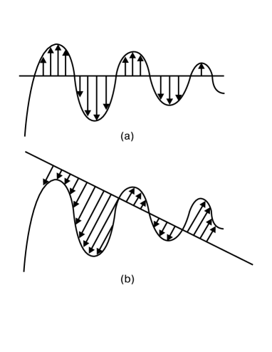
Figure 2: The perturbations (a) and (b) connected by the gauge transformations.

waited result. Indeed, this reflects the fact that energy and other conserved quantities in GR are not localized. Moreover, the formulae (2.52) and (2.53) are very useful because they give a quantitative and constructive description of the non-localization. See the discussion in subsection 1.2.

The transformations (2.48) and (2.49) are directly connected with a way of mapping a perturbed spacetime onto a given background spacetime (a perturbed solution onto a given solution). In the other words, they are connected with a definition of perturbations with respect to a given background. Let us consider a solution in the geometrical form $\hat{g}^{\mu\nu}(x)$. Next let us map a spacetime onto itself following the prescription at the beginning this subsection. Then we obtain $\hat{g}^{\prime\mu\nu}(x)$. After that we decompose both of the solutions into dynamic and background parts:

$$\hat{g}^{\mu\nu}(x) = \overline{\hat{g}}^{\mu\nu}(x)+\hat{l}^{\mu\nu}(x)\,,$$ (2.54)

$$(\hat{g}^{\prime\mu\nu})(x) = \overline{\hat{g}}^{\mu\nu}(x)+\hat{l}^{\prime\mu\nu}(x)\,.$$ (2.55)

The main property of (2.54) and (2.55) is that the background metric is the same. Then it turns out that $\hat{l}^{\mu\nu}(x)$ and $\hat{l}^{\prime\mu\nu}(x)$ are connected by the transformations in (2.48). This situation is interpreted as follows. The same background in (2.54) and (2.55) is chosen by different ways that symbolically is illustrated on the figure 2. The curves in both the cases (a) and (b) symbolize the same solution of GR in the geometrical form, whereas the straight lines present a background, say, a Minkowski space. The perturbations in the cases (a) and (b) are different, but they are solutions to the equations of the field formulation connected by the gauge transformations, and, thus, they are the same solution in different forms. In spite of that the gauge transformations in the field formulation have the evident geometrical origin, they can be interpreted as inner gauge transformations, like in standard gauge theories. Indeed, they act only onto the dynamical variables (perturbations), whereas the backgrounds variables and coordinates do not change.

As discussed in Introduction, in many of applications it is important to consider equations and gauge transformations in linear and quadratic approximations. Assume that perturbations and their derivatives are small: $\hat{l}^{\mu\nu}\ll\overline{\hat{g}}^{\mu\nu}$, $\phi^{A}\ll\overline{\Phi}^{A}$, $\hat{l}^{\mu\nu}\approx\partial_{\alpha}\hat{l}^{\mu\nu}\ldots$ and $\phi^{A}\approx\partial_{\alpha}\phi^{A}\approx\ldots~{}$. Assuming that the background equations (2.16) give a connection $\overline{\hat{g}}^{\mu\nu}\approx h(\kappa)\overline{\Phi}^{A}$ with a coefficient $h(\kappa)$ depending on the Einstein constant one has to set ${\hat{l}^{\mu\nu}}\approx h(\kappa){\phi^{A}}$, etc. Now, rewrite the equations (2.23) up to the second order in perturbations:

$$\hat{G}^{L}_{\mu\nu}(\hat{l})+\hat{\Phi}^{L}_{\mu\nu}(\hat{l},~{}\phi)-\kappa\hat{t}^{(tot2)}_{\mu\nu}(\hat{l}\hat{l},~{}\hat{l}\phi,~{}\phi\phi)=0\,.$$ (2.56)

Assuming iterations the perturbations can be expanded as $\hat{l}^{\mu\nu}=\hat{l}^{\mu\nu}_{1}+\hat{l}^{\mu\nu}_{2}+...~{}$, and $\phi^{A}=\phi^{A}_{1}+\phi^{A}_{2}+...~{}$. Then the linear equations acquire the form:

$$\hat{G}^{L}_{\alpha\beta}(\hat{l}_{1})+\hat{\Phi}^{L}_{\alpha\beta}(\hat{l}_{1},~{}\phi_{1})=0\,,$$ (2.57)

whereas the quadratic equations have the form:

$$\hat{G}^{L}_{\alpha\beta}(\hat{l}_{2})+\hat{\Phi}^{L}_{\alpha\beta}(\hat{l}_{2},~{}\phi_{2})-\kappa\left(\hat{t}^{(gr2)}_{\alpha\beta}(\hat{l}_{1}\hat{l}_{1})+\hat{t}^{(m2)}_{\alpha\beta}(\hat{l}_{1}\hat{l}_{1},~{}\hat{l}_{1}\phi_{1},~{}\phi_{1}\phi_{1})\right)=0\,.$$ (2.58)

Besides, assuming $\xi^{\mu}=\xi_{1}^{\mu}+\xi_{2}^{\mu}+...$ with $\xi_{1}^{\mu}\approx\partial_{\alpha}\xi_{1}^{\mu}\approx\ldots\approx\hat{l}^{\mu\nu}_{1}\approx h(\kappa)\phi^{A}_{1}$ and $\xi_{2}^{\mu}\approx\partial_{\alpha}\xi_{2}^{\mu}\approx\ldots\approx\hat{l}^{\mu\nu}_{2}\approx h(\kappa)\phi^{A}_{2}$, one has a linear version of (2.48) in the simple form:

$$\hat{l}^{\prime\mu\nu}_{1} = \hat{l}^{\mu\nu}_{1}+{{\hbox{$\pounds$}}}_{\xi_{1}}\overline{\hat{g}}^{\mu\nu}=\hat{l}^{\mu\nu}_{1}+\overline{D}^{\mu}\hat{\xi}_{1}^{\nu}+\overline{D}^{\nu}\hat{\xi}_{1}^{\mu}-\overline{\hat{g}}^{\mu\nu}~{}\overline{D}_{\rho}\xi_{1}^{\rho}\,,$$ (2.59)

$$\phi^{\prime A}_{1} = \phi^{A}_{1}+{{\hbox{$\pounds$}}}_{\xi_{1}}\overline{\Phi}^{A}.$$ (2.60)

Under these transformations the equations (2.57) are transformed as

$$\left[\hat{G}^{L}_{\mu\nu}+\hat{\Phi}^{L}_{\mu\nu}\right]^{\prime}=\left[\hat{G}^{L}_{\mu\nu}+\hat{\Phi}^{L}_{\mu\nu}\right]$$ (2.61)

$$+ \left(\sqrt{-\overline{g}}\delta^{\rho}_{\mu}\delta^{\sigma}_{\mu}-{\textstyle{1\over 2}}\overline{g}_{\mu\nu}\overline{\hat{g}}^{\rho\sigma}\right){{\hbox{$\pounds$}}}_{\xi_{1}}\left[\overline{R}_{\rho\sigma}-\kappa\left(\overline{T}_{\rho\sigma}-{\textstyle{1\over 2}}\overline{g}_{\rho\sigma}\overline{T}\right)\right]$$

and are, thus, gauge invariant on the background equations. In the simple case of the Ricci-flat background (2.18) the linear transformations have only the form (2.59), without (2.60). Then the formula (2.61) transfers to the formula $\hat{G}^{\prime L}_{\mu\nu}=\hat{G}^{L}_{\mu\nu}$, which expresses the gauge invariance of the linear field of spin 2. It is the well known gauge transformations in the linear gravity [1, 3].

The quadratic order of the gauge transformations has a form;

$$\hat{l}^{\prime\mu\nu}_{2} = \hat{l}^{\mu\nu}_{2}+{{\hbox{$\pounds$}}}_{\xi_{2}}\overline{\hat{g}}^{\mu\nu}+{1\over{2!}}{{\hbox{$\pounds$}}}^{2}_{\xi_{1}}\overline{\hat{g}}^{\mu\nu}+{{\hbox{$\pounds$}}}_{\xi_{1}}\hat{l}^{\mu\nu}_{1}$$

$$\phi^{\prime A}_{2} = \phi^{A}_{2}+{{\hbox{$\pounds$}}}_{\xi_{2}}\overline{\Phi}^{A}+{1\over{2!}}{{\hbox{$\pounds$}}}^{2}_{\xi_{1}}\overline{\Phi}^{\mu\nu}+{\hbox{$\pounds$}}_{\xi_{1}}\phi^{A}_{1}\,.$$ (2.62)

Substitution of Eqs. (2.59) and (2.62) into (2.58) give

$$\left[\hat{G}^{L}_{\mu\nu}(\hat{l}_{2})+\hat{\Phi}^{L}_{\mu\nu}(\hat{l}_{2},~{}\phi_{2})-\kappa\hat{t}^{(tot2)}_{\mu\nu}\right]^{\prime}=\left[\hat{G}^{L}_{\mu\nu}(\hat{l}_{2})+\hat{\Phi}^{L}_{\mu\nu}(\hat{l}_{2},~{}\phi_{2})-\kappa\hat{t}^{(tot2)}_{\mu\nu}\right]$$ (2.63)

$$+ {{\partial\overline{\hat{g}}^{\rho\sigma}}\over{\partial\overline{g}^{\mu\nu}}}\left({\hbox{$\pounds$}}_{\xi_{2}}+{1\over 2!}{\hbox{$\pounds$}}^{2}_{\xi_{1}}\right)\left[\overline{R}_{\rho\sigma}-\kappa\left(\overline{T}_{\rho\sigma}-{\textstyle{1\over 2}}\overline{g}_{\rho\sigma}\overline{T}\right)\right]+$$

$$+ {{\partial\overline{\hat{g}}^{\rho\sigma}}\over{\partial\overline{g}^{\mu\nu}}}{\hbox{$\pounds$}}_{\xi_{1}}\left[{{\partial\overline{g}^{\delta\pi}}\over{\partial\overline{\hat{g}}^{\rho\sigma}}}\left[\hat{G}^{L}_{\delta\pi}(\hat{l}_{1})+\hat{\Phi}^{L}_{\delta\pi}(\hat{l}_{1},~{}\phi_{1})\right]\right].$$

Thus, equations (2.58) are gauge invariant on the background equations (2.16) and on the linear equations (2.57). Of course, the procedure can be continued in the next orders.

In this subsection, we were based on the exact theory of gauge transformations developed in our works [100, 104]. Together with this, for the presentation we have used some of details given in [101, 112, 113]. An arising interest to cosmological perturbations stimulates their more detailed study including a second order approximation [14]. Thus it turns out necessary to examine the gauge transformations up to a second order also. Such studies (independently on ours, but repeating them in main properties) were carried out, for examples, in [141, 142].

2.7 Differential conservation laws on special backgrounds

The energy-momentum tensor is the one of important objects of a field theory in Minkowski space. Its differential conservation together with symmetries of the Minkowski space permit to construct integral conserved quantities (see subsection 3.2). The field formulation of GR has also the conserved energy-momentum in Minkowski space with the same properties (2.3). In this short subsection we demonstrate that the conservation law, like (2.3), also has a place on curved backgrounds, which are important in many applications. Although conservation laws and conserved quantities are constructed and studied in the next section 3 in detail, by the logic of the presentation we include this subsection here.

Firstly, consider Ricci-flat (including flat) backgrounds (2.18), which have an independent meaning. This means that $\overline{\Phi}^{A}\equiv 0$ and $\overline{{\hat{\cal L}}^{M}}\equiv 0$. Then the Lagrangian (2.19) is simplified to

$${{\hat{\cal L}}}^{dyn}=-{1\over{2\kappa}}{\hat{\cal L}}^{g}+{\hat{\cal L}}^{m}=-{1\over{2\kappa}}{\hat{\cal L}}^{g}+{{\hat{\cal L}}}^{M}\left(\phi^{A};~{}\overline{\hat{g}}^{\mu\nu}+\hat{l}^{\mu\nu}\right).$$ (2.64)

The field equations (2.23) transform into the form

$$\hat{G}^{L}_{\mu\nu}=\kappa\left({\hat{t}}^{g}_{\mu\nu}+{\hat{t}}^{m}_{\mu\nu}\right)\equiv\kappa{\hat{t}}^{(tot)}_{\mu\nu}\,.$$ (2.65)

For (2.18) one has identically $\overline{D}_{\nu}{\hat{G}}^{L\nu}_{\mu}\equiv 0$ and, thus, a divergence of Eq. (2.65) leads to the differential conservation law:

$$\overline{D}_{\nu}{\hat{t}}^{(tot)\nu}_{\mu}=0\,.$$ (2.66)

Now consider backgrounds presented by Einstein spaces in Petrov’s definition [143], then the background equations are

$$\overline{R}_{\mu\nu}=\Lambda\overline{g}_{\mu\nu}\,$$ (2.67)

where $\Lambda$ is a constant. Ricci-flat and AdS backgrounds are particular cases of Einstein’s spaces. The Lagrangian of the background system has the form:

$$\overline{{\hat{\cal L}}^{E}}=-{1\over{2\kappa}}\overline{\hat{R}}+\overline{{\hat{\cal L}}^{M}}=-{1\over{2\kappa}}\left(\overline{\hat{R}}-2\Lambda\sqrt{-\bar{g}}\right)\,.$$ (2.68)

Here, the constant $\Lambda$ is rather interpreted as ‘degenerated’ matter. Then, the dynamical Lagrangian (2.19) transforms into

$${{\hat{\cal L}}}^{dyn}=-{1\over{2\kappa}}{\hat{\cal L}}^{g}+{\hat{\cal L}}^{m}=-{1\over{2\kappa}}{\hat{\cal L}}^{g}+\left[{{\hat{\cal L}}}^{M}\left(\phi^{A};~{}\overline{\hat{g}}^{\mu\nu}+\hat{l}^{\mu\nu}\right)-\hat{l}^{\mu\nu}{{\delta\overline{{\hat{\cal L}}^{M}}}\over{\delta\overline{\hat{g}}^{\mu\nu}}}-{\overline{{\hat{\cal L}}^{M}}}\right]$$ (2.69)

and leads to the field equations (2.23) in the simple form:

$$\hat{G}^{L}_{\mu\nu}+\Lambda\hat{l}^{\mu\nu}=\kappa\left({\hat{t}}^{g}_{\mu\nu}+{\hat{t}}^{m}_{\mu\nu}\right)\equiv\kappa{\hat{t}}^{(tot)}_{\mu\nu}\,.$$ (2.70)

Taking into account the background equations (2.67) one has identically

$$\overline{D}_{\nu}\left(\hat{G}^{L\nu}_{\mu}+\Lambda\hat{l}_{\mu}^{\nu}\right)\equiv 0.$$ (2.71)

Thus, the differentiation of Eq. (2.70) gives the same conservation law (2.66). In heuristic form the differential conservation law on AdS and de Sitter (dS) backgrounds was used in [68]; in the Lagrangian description it was shortly noted in [100]; and, in the paper [144], it was studied in more detail.

2.8 Different definitions of metric perturbations

In GR, the metric perturbations can be defined by different decompositions:

$$g_{\mu\nu} = \overline{g}_{\mu\nu}+h_{\mu\nu},$$

$$\hat{g}^{\mu\nu} = \overline{\hat{g}}^{\mu\nu}+\hat{l}^{\mu\nu},$$

$$g^{\mu\nu} = \overline{g}^{\mu\nu}+r^{\mu\nu},$$

$$\ldots = \ldots+\ldots\,,$$ (2.72)

not only by (2.13). Denoting components of metrical densities in the united way

$$g^{a}=\left\{g^{\mu\nu},~{}g_{\mu\nu},~{}\sqrt{-g}g^{\mu\nu},~{}\sqrt{-g}g_{\mu\nu},~{}(-g)g^{\mu\nu},~{}\ldots\right\}$$ (2.73)

we rewrite the action of GR as

$$S={1\over c}\int d^{4}x{\hat{\cal L}}^{E(a)}\equiv-{1\over{2\kappa c}}\int d^{4}x\hat{R}(g^{a})+{1\over c}\int d^{4}x{\hat{\cal L}}^{M}(\Phi^{A},~{}g^{a})\,.$$ (2.74)

After its variation the Einstein equations take the generalized form:

$$-{1\over 2\kappa}{{\delta\hat{R}}\over{\delta g^{a}}}+{{\delta{\hat{\cal L}}^{M}}\over{\delta g^{a}}}=0\,.$$ (2.75)

The background action and equations have the corresponding to (2.74) and (2.75) barred form. After that we present the united form for decompositions (2.72)

$$g^{a}=\overline{g}^{a}+h^{a}\,,$$ (2.76)

and, following the rules of (2.19), construct the generalized dynamical Lagrangian:

$${{\hat{\cal L}}}^{dyn}_{(a)}=-{1\over{2\kappa}}\hat{R}\left(\overline{g}^{a}+h^{a}\right)+{{\hat{\cal L}}^{M}}\left(\overline{\Phi}^{A}+\phi^{A};~{}\overline{g}^{a}+h^{a}\right)$$ (2.77)

$$- h^{a}\left(-{1\over{2\kappa}}{{\delta\overline{\hat{R}}}\over{\delta\overline{g}^{a}}}+{{\delta{\overline{{\hat{\cal L}}^{M}}}}\over{\delta\overline{g}^{a}}}\right)-\phi^{A}{{\delta{\overline{{\hat{\cal L}}^{M}}}}\over{\delta\overline{\Phi}^{A}}}-\left(-{1\over{2\kappa}}\overline{\hat{R}}+{\overline{{\hat{\cal L}}^{M}}}\right)-{1\over{2\kappa}}\partial_{\nu}\hat{k}^{\nu}.$$

The total symmetrical energy-momentum tensor density is defined as usual:

$${\hat{t}}^{(tot~{}a)}_{\mu\nu}\equiv 2{{\delta{\hat{\cal L}}^{dyn}_{(a)}}\over{\delta\overline{g}^{\mu\nu}}}\,.$$ (2.78)

After substituting the expression (2.77) into this definition (identity) and taking into account Eq. (2.75) and the barred Eq. (2.75) we obtain the Einstein equations in the form (2.23):

$$\hat{G}^{L(a)}_{\mu\nu}+\hat{\Phi}^{L(a)}_{\mu\nu}=\kappa{\hat{t}}^{(tot~{}a)}_{\mu\nu}\,.$$ (2.79)

Here, the linear left hand side is defined by the same operators (2.24) - (2.26), only now with independent variables

$$\hat{l}^{\mu\nu}_{(a)}\equiv h^{a}{{\partial\overline{\hat{g}}^{\mu\nu}}\over{\partial\overline{g}^{a}}}\,.$$ (2.80)

However, a choice of two different arbitrary decompositions as $g^{a}_{1}=\overline{g}^{a}_{1}+h^{a}_{1}$ and $g^{a}_{2}=\overline{g}^{a}_{2}+h^{a}_{2}$, gives the difference

$$\hat{l}^{\mu\nu}_{(a2)}-\hat{l}^{\mu\nu}_{(a1)}=\hat{\beta}^{\mu\nu}_{(a)12}\,,$$ (2.81)

which is not less than quadratic in perturbations. Because differences enter the linear expressions of equations (2.79) the energy-momentum tensor densities ${\hat{t}}^{(tot~{}1a)}_{\mu\nu}$ and ${\hat{t}}^{(tot~{}2a)}_{\mu\nu}$ have the same differences too. For the case of flat backgrounds this ambiguity was noted by Boulware and Deser [145]. Later we [104] have examined it for arbitrary curved backgrounds and arbitrary metric theories. However, only in our works [116, 118] this ambiguity has been resolved, and we present this solution in subsection 3.5.

3 Conservation laws in GR

3.1 Classical pseudotensors and superpotentials

During many decades after constructing GR pseudotensors and superpotentials were main objects in constructing conservation laws and conserved quantities. In the framework of the field-theoretical approach these notions and quantities, in a definite sense, are developed and generalized. Therefore in this subsection we give a short review describing classical pseudotensors and superpotentials, only which are necessary in our own presentation. On their examples we outline the general properties of such objects, their problems and some of modern applications.

Let us present the general way for constructing pseudotensors and superpotentials. Using the metric and its derivations construct an arbitrary quantity $\hat{\cal U}^{\mu\alpha}_{\nu}$, satisfying the condition

$$\partial_{\mu\alpha}\hat{\cal U}^{\mu\alpha}_{\nu}\equiv 0\,.$$ (3.1)

Next, define the complex

$$\hat{\theta}^{\mu}_{\nu}\equiv\partial_{\alpha}\hat{\cal U}^{\mu\alpha}_{\nu}-\frac{1}{\kappa}\hat{G}^{\mu}_{\nu}\,,$$ (3.2)

which usually is called as an energy-momentum pseudotensor of gravitational field. Using the Einstein equations one obtains

$$\hat{T}_{\nu}^{\mu}+\hat{\theta}_{\nu}^{\mu}=\partial_{\alpha}\hat{\cal U}^{\mu\alpha}_{\nu}\,$$ (3.3)

where $\hat{\cal U}^{\mu\alpha}_{\nu}$ plays the role of a superpotential. Thus Eq. (3.3) is another form of the Einstein equations. Due to (3.1) one has a differential conservation law

$$\partial_{\mu}\left(\hat{T}_{\nu}^{\mu}+\hat{\theta}_{\nu}^{\mu}\right)=0\,.$$ (3.4)

Concerning the physical sense, it is the 4-dimensional continuity equation, which is the differential conservation law derived directly from the field equations. As is seen, the above construction has problems. First, it is an ambiguity in a definition of $\hat{\theta}_{\nu}^{\mu}$ and $\hat{\cal U}^{\mu\alpha}_{\nu}$, second, these expressions are not covariant in general.

The presented picture, as a generalization, has been formulated after prolonged history of constructing pseudotensors and superpotentials in GR (see a review [146]). Below we recall constructing some of well known expressions. In the work [55], following the standard rules Einstein had suggested his famous pseudotensor. Firstly, a non-covariant Lagrangian

$${\hat{\cal L}}^{cut}=-\frac{1}{2\kappa}\hat{g}^{\mu\nu}\left(\Gamma^{\sigma}_{\mu\rho}\Gamma^{\rho}_{\sigma\nu}-\Gamma^{\rho}_{\mu\nu}\Gamma^{\sigma}_{\rho\sigma}\right)$$ (3.5)

had been suggested. It differs from the covariant Hilbert Lagrangian

$${\hat{\cal L}}^{H}=-\frac{1}{2\kappa}\hat{R}$$ (3.6)

by a divergence and leads to the same field equations (2.12). Next, the corresponding to (3.5) canonical complex had been constructed:

$$\hat{t}_{\nu}^{E\mu}={\frac{\partial{\hat{\cal L}}^{cut}}{\partial(\partial_{\mu}g_{\alpha\beta})}}\partial_{\nu}g_{\alpha\beta}-\delta^{\mu}_{\nu}{\hat{\cal L}}^{cut}\,,$$ (3.7)

which is just the Einstein pseudotensor. Both the Lagrangian (3.5) and the pseudotensor (3.7) depend on the metric $g_{\mu\nu}$ and only its first derivatives. Combining (3.7) and the field equations Einstein had obtained the conservation law

$$\partial_{\mu}\left(\hat{T}_{\nu}^{\mu}+\hat{t}_{\nu}^{E\mu}\right)=0\,,$$ (3.8)

which is a variant of (3.4).

Later Tolman [147] had found the quantity $\hat{\cal T}^{\mu\alpha}_{\nu}$ with a property (3.1), and for which, as a particular case of (3.3), one has $\hat{T}_{\nu}^{\mu}+\hat{t}_{\nu}^{E\mu}\equiv\partial_{\alpha}\hat{\cal T}^{\mu\alpha}_{\nu}$. From here the conservation law (3.8) follows directly. However, $\hat{\cal T}^{\mu\alpha}_{\nu}$ is not antisymmetrical in $\alpha$ and $\beta$, whereas the use of antisymmetrical superpotentials ${\cal U}^{\mu\alpha}_{\nu}=-{\cal U}^{\alpha\mu}_{\nu}$ is more reasonable because it makes explicit the identity (3.1) and presents less difficulties under covariantization, etc. Assuming an antisymmetry Freud [148] had found out the superpotential

$$\hat{\cal F}^{\mu\alpha}_{\nu}\equiv\frac{1}{2\kappa}\frac{g_{\nu\rho}}{\sqrt{-g}}\partial_{\lambda}\left[(-g)\left(g^{\mu\rho}g^{\alpha\lambda}-g^{\mu\lambda}g^{\alpha\rho}\right)\right]\,,$$ (3.9)

such that

$$\hat{T}_{\nu}^{\mu}+\hat{t}_{\nu}^{E\mu}=\partial_{\alpha}\hat{\cal F}^{\mu\alpha}_{\nu},$$ (3.10)

and connected with the Tolman one by $\hat{\cal F}^{\mu\alpha}_{\nu}\equiv\hat{\cal T}^{\mu\alpha}_{\nu}+\partial_{\beta}\hat{\Phi}^{\mu\alpha\beta}_{\nu}$; $\partial_{\alpha\beta}\hat{\Phi}^{\mu\alpha\beta}_{\nu}\equiv 0.$

Many authors (see, e.g., more known publications [149] - [151] and the review [146]) considered the problem of an ambiguity in definition of conserved quantities described in (3.1) - (3.4). It has turned out that some of pseudotensors and superpotentials are directly connected with a Lagrangian through the Nœther procedure. This restricts some ambiguities in their definitions. Naturally, the Eienstein pseudotensor is defined by the Lagrangian (3.5) which, being generally non-covariant, is covariant with respect to linear coordinate transformations. Then for translations $\lambda^{\mu}_{(\alpha)}=\delta^{\mu}_{\alpha}$ one can write out the Nœther identity:

$${\pounds}_{\lambda}{\hat{\cal L}}^{cut}+\partial_{\mu}\left(\lambda^{\mu}_{(\alpha)}{\hat{\cal L}}^{cut}\right)\equiv 0\,.$$ (3.11)

Direct calculations lead to $\partial_{\mu}\left({\kappa}^{-1}\hat{G}_{\nu}^{\mu}+\hat{t}_{\nu}^{E\mu}\right)\equiv 0$ with the definition (3.7) that after using Eq. (2.12) gives the conservation law (3.8). The general conclusion is formulated as follows.

• In the sense of the Nœther procedure the pseudotensor (3.7) is uniquely defined by the Lagrangian (3.5); other Lagrangians ${\hat{\cal L}}={\hat{\cal L}}^{cut}+div$ lead to other pseudotensors.

Thus the identity (3.11) with the Hilbert Lagrangian (3.6) leads to

$$\hat{T}_{\nu}^{\mu}+\hat{\cal M}_{\nu}^{\mu}=\partial_{\alpha}\hat{\chi}^{\mu\alpha}_{\nu}\,,$$ (3.12)

instead of (3.10), where the Møller [151] superpotential

$$\hat{\chi}^{\mu\alpha}_{\nu}\equiv{1\over 2\kappa}\sqrt{-g}g^{\mu\beta}g^{\alpha\rho}\left(\partial_{\beta}g_{\nu\rho}-\partial_{\rho}g_{\nu\beta}\right)$$ (3.13)

is used. The components $\hat{\cal M}^{0}_{\nu}(x^{\alpha})$ of the pseudotensor in Eq. (3.12) are transformed as a 4-dimensional vector density under transformations $x^{\prime k}=f^{k}(x^{l})$, $x^{\prime 0}=x^{0}+g(x^{l})$ [151]. In contrary, the corresponding components of the Einstein pseudotensor (3.7) do not. This property of $\hat{\cal M}^{0}_{\nu}(x^{\alpha})$, in a part, improves the general non-covariant picture.

The other problem is in a definition of angular momentum of a system. Both Einsten’s and Mœller’s pseudotensors themselves, as canonical Nœther complexes, cannot define it. One needs to modify these expressions or to construct new ones (see the review [146]). One of methods to construct angular momentum, using unique energy-momentum complex, is to construct symmetrical pseudotensors. Thus, Landau and Lifshitz have suggested a such expression [1]. Their famous symmetrical pseudotensor ${{t}}_{LL}^{\mu\nu}$, like $\hat{t}_{\mu}^{E\nu}$, has only the first derivatives, and is expressed through Einstein’s (3.7) and the Freud’s (3.9) expressions: ${}{{t}}_{LL}^{\mu\nu}=\hat{g}^{\mu\sigma}_{~{}~{},\rho}\hat{\cal F}^{[\nu\rho]}_{\sigma}+\hat{g}^{\mu\rho}{}\hat{t}_{\rho}^{E\nu}$. However, as is seen, it has an anomalous weight $+2$, unlike expressions in (3.10) and (3.12) with the weight $+1$. Goldberg [150] generalized the Landau-Lifshitz approach, suggesting a symmetrical pseudotensor of an arbitrary weight.

Concerning symmetrical expressions, return also to the the equation (2.1) and the expression (2.2). The last can be rewritten as

$$\hat{G}_{L}^{\mu\nu} \equiv \kappa\partial_{\beta}\hat{\cal P}^{\mu[\nu\beta]}\,,$$ (3.14)

$$\hat{\cal P}^{\mu[\nu\beta]} \equiv \frac{1}{\kappa}\partial_{\alpha}\left(\hat{l}^{\nu[\mu}\eta^{\alpha]\beta}-\hat{l}^{\beta[\mu}\eta^{\alpha]\nu}\right)\,.$$ (3.15)

One can find that $\hat{\cal P}^{\mu[\nu\beta]}$ is the well known superpotential by Papapetrou [152]; in the linear approximation it is Weinberg’s superpotential [153]; and, up to factor $\sqrt{-\eta}$, it coincides also with the linear version of the Landau-Lifshitz superpotential [1]. Then the equation (2.1) can be rewritten as

$$\hat{t}_{(tot)}^{\mu\nu}=\partial_{\beta}\hat{\cal P}^{\mu[\nu\beta]}\,.$$ (3.16)

This means that the conservation law (2.3) can be interpreted by the same way as the conservation law (3.4), i.e. in the framework of the superpotential approach.

It was a problem to relate modified superpotentials to Lagrangians, like it was done for Freud’s (3.9) and Møller’s (3.13) ones. Only recently with the use of a covariant Hamiltonian formalism [94] (see subsection 1.2) Chang, Nester and Chen [95] closed this gap. They describe GR by Hamiltonians with different surface terms corresponding to different boundary conditions under variation. For each of known (covariantized) superpotentials one can find its own Hamiltonian. Thus, the Dirichlet conditions correspond to the Freud superpotential (3.9), Neuman’s ones — to Møller’s superpotential (3.13). All the other superpotentials require more complicated boundary conditions. Recently Babak and Grishchuk [122] suggested a special Lagrangian including additional terms with Lagrangian multipliers, which leads to a covariantized Landau-Lifshitz pseudotensor of normal weight $+1$.

Of course, a non-covariance of pseudotensors and superpotentials lead to the evident problems described in all the textbooks. In this relation, return to the Hilbert Lagrangian (3.6) recalling that it is generally covariant. Thus, for constructing conservation laws one can use arbitrary diplacement vectors $\xi^{\mu}$, not just the linear translations $\lambda^{\mu}_{(\alpha)}$, like in (3.11). Hence there has to exist a generally covariant energy-momentum complex and superpotential. Such quantities were found by Komar [154], his superpotential is

$$\hat{\cal K}^{[\mu\alpha]}={{\sqrt{-g}}\over 2\kappa}\left(D^{\mu}\xi^{\alpha}-D^{\alpha}\xi^{\mu}\right)={{\sqrt{-g}}\over\kappa}D^{[\mu}\xi^{\alpha]}={{1}\over\kappa}D^{[\mu}\hat{\xi}^{\alpha]}\,.$$ (3.17)

With $\xi^{\mu}=\rm const$ it goes to the Møller superpotential (3.13). However, in spite of the advantage with covariance, there are problems. The superpotential (3.17) does not make a correct ratio of angular momentum to mass in the Kerr solution (see, e.g., [137, 140]).

The mentioned above problems could be neglected if resonable assumptions are made. Then many classical pseudotensors and superpotentials could be useful for a description of differerent physical systems. In this sense it is useful to return to Einstein’s arguments. First, in spite of that the local conservation laws (3.8) are not covariant they have the same form in every coordinate system. Being the continuity equations they give a balance between a loss and a gain of a density of particularly defined physical quantities, and hence they state the equilibrium of a system. The second remarkable Einstein’s example [59] is related to masses connected by a rigid rod. Tensions in the road (which exist because $\hat{T}^{\mu}_{\nu}$ is present in (3.8)) can be interpreted only as a compensation to tensions of gravitational field included in $t_{\mu}{}^{E\nu}$. Third, Einstein had suggested also a simple method for the “localization” [58], when an isolated system is considered as placed into “Galileian space”, and “Galileian coordinates” are used for description. Finally, he had used his energy-momentum complex to describe weak gravitational waves as metric perturbations with respect to a Mikowski metric [56] - [58].

At reasonable assumptions, pseudotensors and superpotentials are left useful nowadays too. Thus, usually quantities of global energy-momentum and angular momentum for asymptotically flat spacetimes are calculated. For example, Bergmann-Tomson’s and Landau-Lifshitz’s complexes give the same expressions for global angular momentum in an isolated system [155]. In [156, 157], with the use of the Einstein, Tolman and Landau-Lifshitz complexes reasonable energy and momentum densities of cylindrical gravitational waves were obtained. Recently, in the work [158] with a careful set of assumptions it was shown that a tidal work in GR calculated for different non-covariant energy-momentum complexes is the same and unambiguous. Authors frequently use pseudotensors and superpotentials to describe many popular exact solutions of GR (see [159] - [166] and references there in). Particulary, it was shown that in many cases different pseudotensors give the same energy distribution for the same solution.

However, in spite of some successes in applying pseudotensors and superpotentials, it is clear that more universal and unambiguous quantities are more preferable. The next subsection is devoted to possible ways in improving properties of the classical complexes.

3.2 Requirements for constructing conservation laws on curved backgrounds

From the beginning we recall how conservation laws are constructed in a field theory in a Minkowski space. These principles are useful both to understand how classical pseudotensors and superpotentials could be modified to avoid their problems and to better describe and explain conservation laws in the field-theoretical formulation.

Consider an arbitrary theory of fields $\psi^{A}$ in the Minkowski space in curved coordinates with the Lagrangian

$${\hat{\cal L}}_{(\psi)}={\hat{\cal L}}_{(\psi)}\left(\psi^{A},\overline{D}_{\alpha}\psi^{A},\overline{g}_{\mu\nu}\right)\,.$$ (3.18)

For the sake of simplicity assume that it contains the first derivatives only. The symmetrical (metric) energy-momentum tensor density is defined as usual:

$$\hat{t}_{(s)\alpha\beta}\equiv 2{{\delta{\hat{\cal L}}_{(\psi)}}\over{\delta\overline{g}^{\alpha\beta}}}\,.$$ (3.19)

The density of the canonical energy-momentum tensor has the form:

$$\hat{t}^{\alpha}_{(c)\sigma}\equiv{{\partial{\hat{\cal L}}_{(\psi)}}\over{\partial\left(\overline{D}_{\alpha}\psi^{A}\right)}}\overline{D}_{\sigma}\psi^{A}-{\hat{\cal L}}_{(\psi)}\delta^{\alpha}_{\sigma}\,.$$ (3.20)

Both of them are differentially conserved

$$\overline{D}_{\alpha}\hat{t}^{\alpha}_{(s)\sigma} = 0\,,$$ (3.21)

$$\overline{D}_{\alpha}\hat{t}^{\alpha}_{(c)\sigma} = 0\,,$$ (3.22)

on the field equations. To construct integral conserved quantities it is necessary to use Killing vectors of the Minkowski space. Contracting $\hat{t}^{\alpha}_{(s)\sigma}$ with an each of the 10 Killing vectors $\lambda^{\nu}$ one obtains the currents

$$\hat{I}^{\mu}_{(s)}(\lambda)\equiv\hat{t}^{\mu}_{(s)\nu}\lambda^{\nu}\,,$$ (3.23)

which are conserved differentially

$$\overline{D}_{\alpha}\hat{I}^{\alpha}_{(s)}(\lambda)\equiv\partial_{\alpha}\hat{I}^{\alpha}_{(s)}(\lambda)=0\,.$$ (3.24)

The other situation with the canonical energy-momentum $\hat{t}^{\alpha}_{(c)\sigma}$. If one tries to contract it with the 4-rotation Killing vectors, then the correspondent currents, like (3.23), are not conserved. The reason is that $\hat{t}^{\alpha\sigma}_{(c)}$ is not symmetrical in general. A one of the ways to construct differentially conserved currents is

$$\hat{I}^{\alpha}_{(c)}(\lambda)\equiv\hat{t}^{\alpha}_{(c)\sigma}\lambda^{\sigma}+\hat{\sigma}^{\alpha\beta}_{(\psi)}{}_{\sigma}\overline{D}_{\beta}\lambda^{\sigma}\,$$ (3.25)

where

$$\hat{\sigma}^{\alpha\beta}_{(\psi)}{}_{\sigma}\equiv-{{\partial{\hat{\cal L}}_{(\psi)}}\over{\partial\left(\overline{D}_{\alpha}\psi^{A}\right)}}\left.\psi^{A}\right|^{\beta}_{\sigma}\,$$ (3.26)

is a spin density. Another way follows the Belinfante symmetrization [167], who has introduced the antisymmetric in $\alpha$ and $\beta$ expression

$$\hat{S}^{\alpha\beta\gamma}_{(\psi)}=\hat{\sigma}^{\gamma[\alpha\beta]}_{(\psi)}+\hat{\sigma}^{\alpha[\gamma\beta]}_{(\psi)}-\hat{\sigma}^{\beta[\gamma\alpha]}_{(\psi)}\,$$ (3.27)

and has defined the new (symmetrized) energy-momentum tensor density as follows

$$\hat{t}^{\alpha}_{(B)\sigma}=\hat{t}^{\alpha}_{(c)\sigma}+\overline{D}_{\beta}\hat{S}^{\alpha\beta}_{(\psi)\sigma}.$$ (3.28)

It is also conserved, $\overline{D}_{\alpha}\hat{t}^{\alpha}_{(B)\sigma}=0$, on the equations of motion. Besides, it is symmetrical on the equations of motion. Then the symmetrized current

$$\hat{I}^{\alpha}_{(B)}(\lambda)\equiv\hat{t}^{\alpha}_{(B)\sigma}\lambda^{\sigma}\,$$ (3.29)

is also conserved for all the Killing vectors, i.e. one can use the unique object $\hat{t}^{\alpha}_{(B)\sigma}$ without additional quantities, like the spin tensor in (3.25).

For the Minkowski background it is easy to show

$$\hat{t}_{(s)\sigma}^{\alpha}=\hat{t}^{\alpha}_{(c)\sigma}+\overline{D}_{\beta}\hat{S}^{\alpha\beta}_{(\psi)\sigma}=\hat{t}^{\alpha}_{(B)\sigma}\,$$ (3.30)

on the field equations. Thus the metric energy-momentum (3.19) is equivalent to the Belinfante symmetrized quantity (3.28) (in this relation see also [168]), i.e. $\hat{I}^{\mu}_{(s)}=\hat{I}^{\mu}_{(B)}$. Note also that $\hat{I}^{\mu}_{(s)}$ differs from $\hat{I}^{\mu}_{(c)}$ by a divergence. One can see that the Belinfante procedure suppresses the spin term in the current (3.25). Classical electrodynamics has just the Lagrangian of the type (3.18), and is a good illustration of the above.

The first example where the Belinfante method was used in GR is the paper by Papapertrou [152]. He has symmetrized the Einstein pseudotensor and obtained his remarkable superpotential. By the original definition [167] it is necessary to use a background metric. Thus, Papapetrou used an auxiliary Minkowski metric. Later Berezin [169], in the framework of the field approach in GR on a flat background, has shown that effective energy-momentum tensor can be constructed by the Belinfante method. Applications of the Belinfante method in GR to the pseudotensors without using an auxiliary background

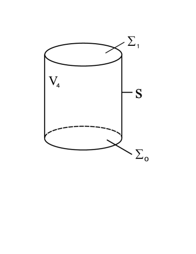
Figure 3: 4-dimensional volume $V_{4}$ restricted by a truncated cylinder.

metric [168, 170] lead uniquely to the Einstein tensor. It is important and interesting result. However, this cannot be useful for description of energy characteristics, e.g., in vacuum case. Recently Borokhov [171] generalized the Belinfante method for an arbitrary field theory on arbitrary backgrounds, with arbitrary Killing vectors and with non-minimal coupling. With simplification to minimal coupling his model goes to the standard description [60, 168, 170].

Denoting $\hat{I}^{\mu}_{(\psi)}=\left\{\hat{I}^{\mu}_{(s)},\,\hat{I}^{\mu}_{(c)}\right\}$ consider 4-dimensional volume $V_{4}$ in the Mikowski space, the boundary of which consists of timelike “wall” $S$ (cylinder) and two spacelike sections: $\Sigma_{0}:=t_{0}=\rm const$ and $\Sigma_{1}:=t_{1}=\rm const$ (see figure 3). Because the conservation laws, like (3.24), are presented by the scalar densities, they can be integrated through the 4-volume: $\int_{V_{4}}\partial_{\mu}\hat{I}^{\mu}_{(\psi)}(\lambda)d^{4}x=0\,.$ The generalized Gauss theorem gives

$$\int_{\Sigma_{1}}\hat{I}^{0}_{(\psi)}(\lambda)d^{3}x-\int_{\Sigma_{0}}\hat{I}^{0}_{(\psi)}(\lambda)d^{3}x+\oint_{S}\hat{I}^{\mu}_{(\psi)}(\lambda)dS_{\mu}=0\,$$ (3.31)

where $dS_{\mu}$ is the element of integration on $S$. If in Eq. (3.31)

$$\oint_{S}\hat{I}^{\mu}_{(\psi)}(\lambda)dS_{\mu}=0\,,$$ (3.32)

then the quantity

$${\cal P}_{(\psi)}(\lambda)=\int_{\Sigma}\hat{I}^{0}_{(\psi)}(\lambda)d^{3}x\,$$ (3.33)

is conserved on $\Sigma$ restricted by $\partial\Sigma$ — intersection of $\Sigma$ with $S$. If the equality (3.32) does not hold, then Eq. (3.31) describes changing the quantity (3.33), i.e. its flux trough $\partial\Sigma$. Due to the difference between $\hat{I}^{\mu}_{(s)}$ and $\hat{I}^{\mu}_{(c)}$ the quantities ${\cal P}_{(s)}(\lambda)$ and ${\cal P}_{(c)}(\lambda)$ differ one from another by surface integrals. However, as a rule, boundary conditions suppress these surface terms, and then ${\cal P}_{(s)}(\lambda)={\cal P}_{(c)}(\lambda)$.

Now let us return to pseudotenors and superpotentials. To avoid some problems they have to be covariantized. Usually a covariantization is carried out by including an auxiliary metric of a Minkowski space. After that partial derivatives are related to Lorentzian coordinates of this flat spacetime. In arbitrary coordinates, partial derivatives naturally transform into covariant ones. Thus, one can keep in mind that in usual expressions, like (3.3) in general form, already there exist the Minkowski metric $\eta_{\mu\nu}$ and its determinant $\eta\equiv\det{\eta_{\mu\nu}}=-1$. For constructing integral conservation laws based on covariantized pseudotensors it is also natural to use the Killing vectors of the Minkowski space.

Let us present the program of the covariantization in detail. Consider the generalized conservation law (3.4) and rewrite it in the equivalent form:

$$\partial_{\mu}\left[\sqrt{-\eta}\left(({\hat{\theta}^{\mu}_{\rho}}+{\hat{T}^{\mu}_{\rho}})/{\sqrt{-\eta}}\right)\lambda^{\rho}_{(\nu)}\right]=0\,.$$ (3.34)

Here, the left hand side is a scalar density. The translation Killing vector $\lambda^{\rho}_{(\nu)}$ of the background Minkowski space is expressed in the Lorentzian coordinates, therefore one has $\lambda^{\rho}_{(\nu)}=\delta^{\rho}_{\nu}$ (the lower index is not coordinate one). Thus, in (3.34) the differentially conserved vector density (current)

$$\hat{\cal J}^{\mu}(\lambda) \equiv \sqrt{-\eta}\left(({\hat{\theta}^{\mu}_{\rho}}+{\hat{T}^{\mu}_{\rho}})/{\sqrt{-\eta}}\right)\lambda^{\rho}_{(\nu)}\,,$$ (3.35)

$$\overline{D}_{\mu}\hat{\cal J}^{\mu}(\lambda) \equiv \partial_{\mu}\hat{\cal J}^{\mu}(\lambda)=0\,$$ (3.36)

is presented. Here, one has to accent that if $\hat{\theta}^{\mu\nu}$ is symmetrical, then the conservation law (3.36) could be extended for 4-rotation Killing vectors. However, if $\hat{\theta}^{\mu\nu}$ is not symmetrical, then the simple and direct covariantization is restricted to using only translation Killing vectors.

Next, as is seen, the programm of constructing integral quantities (3.31) - (3.33) can be repeated for the covariantized current (3.35). The superpotential in Eq. (3.3) can also be rewritten in the covariantized form:

$$\hat{\cal J}^{\mu\alpha}(\lambda)=\sqrt{-\eta}\left({\hat{\cal U}^{\mu\alpha}_{\rho}}/{\sqrt{-\eta}}\right)\lambda^{\rho}_{(\nu)}\,.$$ (3.37)

Thus the expression (3.3) can be rewritten in a fully covariant form:

$$\hat{\cal J}^{\mu}(\lambda)=\partial_{\alpha}\hat{\cal J}^{\mu\alpha}(\lambda)\equiv\overline{D}_{\alpha}\hat{\cal J}^{\mu\alpha}(\lambda)$$ (3.38)

that has a sense of the conservation law because $\hat{\cal J}^{\mu\alpha}(\lambda)$ is an antisymmetric tensor density. Due to antisymmetry of the superpotential (3.37), the 4-momentum presented in the volume form, like (3.33), is expressed as a surface integral

$${\cal P}(\lambda)=\oint_{\partial\Sigma}\hat{\cal J}^{0k}(\lambda)ds_{k}$$ (3.39)

where $ds_{k}$ is the element of integration on $\partial\Sigma$.

Up to now in constructing conservation laws we considered Killing vectors of a background only. However, other displacement vectors can be used also. Let us give two examples. First, for study of perturbations on FRW backgrounds a so-called notion of an integral constraint, which connects a volume integral of only matter perturbations with a surface integral of only metric perturbations, frequently is very important [172]. With the use of such constraints, e.g., measurable effects of the cosmic background radiation were analyzed [173]. In the definition of integral constraints integral constraint vectors, not necessarily Killing vectors, play a crucial role [172]. Second, in [174], a new conserved energy-momentum pseudotensor was found and used in an effort to integrate Einstein’s equations with scalar perturbations and topological defects on FRW backgrounds for a sign of spatial curvature $k=0$. In [175] it was realized that these conservation laws might be associated with the conformal Killing vector of time translation, and can be also generalized for $k=\pm 1$.

Taking into account the above we formulate the generalized requirements for constructing conservation laws for perturbations on curved backgrounds as follows.

• Expressions have to be covariant on a chosen background and valid for arbitrary curved backgrounds.

• One has to construct differentially conserved currents (vector densities) $\hat{\cal J}^{\mu}(\xi)$, such that $\partial_{\mu}\hat{\cal J}^{\mu}(\xi)=0$, and which are defined by the canonical Nœther procedure applied to a Lagrangian of a perturbed system.

• The currents have to be expressed through corresponding superpotentials $\hat{\cal J}^{\mu\nu}$ (antisymmetric tensor densities), such that $\partial_{\mu\nu}\hat{\cal J}^{\mu\nu}(\xi)\equiv 0$, by the way $\hat{\cal J}^{\mu}(\xi)=\partial_{\nu}\hat{\cal J}^{\mu\nu}(\xi)$.

• There has to be a possibility to use arbitrary displacement vectors $\xi^{\mu}$, not only Killing vectors of the background.

• Applications of suggested conserved quantities and conservation laws have to satisfy the known tests (see discussion in subsection 1.2).

3.3 The Katz, Bičák and Lynden-Bell conservation laws

Katz, Bičák and Lynden-Bell [176] (later we call as KBL) have satisfied the requirements at the end of previous subsection. They describe a perturbed system by the Lagrangian:

$${\hat{\cal L}}_{KBL}=\hat{\cal L}^{E}-\overline{{\hat{\cal L}}^{E}}-{1\over 2\kappa}\partial_{\alpha}\hat{k}^{\alpha}\,,$$ (3.40)

see notations in (2.8) and (2.15). In fact they use bimetric formalism, where $g_{\mu\nu}$ and $\overline{g}_{\mu\nu}$ are thought as independent metric coefficients. The gravitational part of (3.40) is

$${\hat{\cal L}}_{G}=-{1\over 2\kappa}\left(\hat{R}-\overline{\hat{R}}+\partial_{\alpha}\hat{k}^{\alpha}\right)\,.$$ (3.41)

Here, for the physical scalar curvature density $\hat{R}$ an external background metric $\overline{g}_{\mu\nu}$ is introduced with the use of the presentation for the curvature tensor:

$$R^{\lambda}{}_{\tau\rho\sigma}=\overline{D}_{\rho}\Delta^{\lambda}_{\tau\sigma}-\overline{D}_{\sigma}\Delta^{\lambda}_{\tau\rho}+\Delta^{\lambda}_{\rho\eta}\Delta^{\eta}_{\tau\sigma}-\Delta^{\lambda}_{\sigma\eta}\Delta^{\eta}_{\tau\rho}+\overline{R}^{\lambda}{}_{\tau\rho\sigma}\,.$$ (3.42)

It is also very important to note that $\hat{k}^{\alpha}$ is defined in (2.20).

For the Lagrangian (3.41), as for a scalar density, one has the identity:

$${\pounds_{\xi}}{\hat{\cal L}}_{G}+\partial_{\mu}\left(\xi^{\mu}{\hat{\cal L}}_{G}\right)\equiv 0\,.$$ (3.43)

It is a generalization of Eq. (3.11) for arbitrary displacement vectors $\xi^{\mu}$. Consequent identical transformations give:

$$\partial_{\mu}\hat{\jmath}^{\mu} \equiv 0\,,$$ (3.44)

$$\hat{\jmath}^{\mu} \equiv \left[{{\partial{\hat{\cal L}}_{G}}\over{\partial\left(\overline{D}_{\mu}g_{\rho\sigma}\right)}}\overline{D}_{\nu}g_{\rho\sigma}-{\hat{\cal L}}_{G}\delta^{\mu}_{\nu}\right]\xi^{\nu}-{{\partial{\hat{\cal L}}_{G}}\over{\partial\left(\overline{D}_{\mu}g_{\rho\sigma}\right)}}\left.g_{\rho\sigma}\right|^{\rho}_{\lambda}\bar{g}^{\lambda\sigma}\overline{D}_{\rho}\xi_{\sigma}$$ (3.45)

$$- {{\delta{{\hat{\cal L}}_{G}}}\over{\delta g_{\rho\sigma}}}\left.{g_{\rho\sigma}}\right|^{\mu}_{\nu}\xi^{\nu}-{{\delta{{\hat{\cal L}}_{G}}}\over{\delta\overline{g}_{\rho\sigma}}}\left.{\overline{g}_{\rho\sigma}}\right|^{\mu}_{\nu}\xi^{\nu}+\hat{Z}^{\mu}_{(c)}\equiv 0\,.$$

Note that here

$$-{{\delta{{\hat{\cal L}}_{G}}}\over{\delta g_{\rho\sigma}}}\left.{g_{\rho\sigma}}\right|^{\mu}_{\nu}\xi^{\nu}\equiv{1\over{\kappa}}{\hat{G}^{\mu}_{\nu}}\xi^{\nu}\,,\qquad-{{\delta{{\hat{\cal L}}_{G}}}\over{\delta\overline{g}_{\rho\sigma}}}\left.{\overline{g}_{\rho\sigma}}\right|^{\mu}_{\nu}\xi^{\nu}\equiv-{1\over{\kappa}}{\overline{\hat{G}}^{\mu}_{\nu}}\xi^{\nu}\,.$$ (3.46)

Then substituting the Einstein equations (2.12) and their barred version into Eq. (3.44) one obtains the differential conservation law

$$\partial_{\mu}\hat{J}^{\mu}_{(c)}(\xi) = 0\,,$$ (3.47)

$$\hat{J}^{\mu}_{(c)}(\xi) \equiv \hat{\Theta}^{\mu}_{(c)\nu}\xi^{\nu}+\hat{\sigma}^{\mu\rho\sigma}\overline{D}_{\rho}\xi_{\sigma}+\hat{Z}^{\mu}_{(c)}(\xi)\,.$$ (3.48)

The first term in (3.48), the generalized total energy-momentum tensor density, is

$$\hat{\Theta}^{\mu}_{(c)\nu}=\hat{t}^{\mu}_{\nu}+\left(\hat{T}^{\mu}_{\nu}-\overline{\hat{T}}^{\mu}_{\nu}\right)+{1\over 2\kappa}\hat{l}^{\rho\sigma}\overline{R}_{\rho\sigma}\delta^{\mu}_{\nu}\,,$$ (3.49)

with $\hat{l}^{\rho\sigma}=\hat{g}^{\rho\sigma}-\overline{\hat{g}}^{\rho\sigma}$. The first term in Eq. (3.49) is the canonical energy-momentum tensor density of the gravitational field:

$$2\kappa\hat{t}^{\mu}_{\nu} = \hat{g}^{\rho\sigma}\left(\Delta^{\lambda}_{\rho\lambda}\Delta^{\mu}_{\sigma\nu}+\Delta^{\mu}_{\rho\sigma}\Delta^{\lambda}_{\lambda\nu}-2\Delta^{\mu}_{\rho\lambda}\Delta^{\lambda}_{\sigma\nu}\right)$$ (3.50)

$$- \hat{g}^{\rho\sigma}\left(\Delta^{\eta}_{\rho\sigma}\Delta^{\lambda}_{\eta\lambda}-\Delta^{\eta}_{\rho\lambda}\Delta^{\lambda}_{\eta\sigma}\right)\delta^{\mu}_{\nu}+\hat{g}^{\mu\lambda}\left(\Delta^{\sigma}_{\rho\sigma}\Delta^{\rho}_{\lambda\nu}-\Delta^{\sigma}_{\lambda\sigma}\Delta^{\rho}_{\rho\nu}\right)\,,$$

the second term in Eq. (3.49) is a perturbation of the matter energy-momentum, the third term describes an interaction with the background. The second term in (3.48) is the spin tensor density:

$$2\kappa\hat{\sigma}^{\mu\rho\sigma}\equiv - 2\kappa{{\partial{\hat{\cal L}}_{G}}\over{\partial\left(\overline{D}_{\mu}g_{\rho\sigma}\right)}}\left.g_{\rho\sigma}\right|^{\rho}_{\lambda}\bar{g}^{\lambda\sigma}=(\hat{g}^{\mu\rho}\overline{g}^{\sigma\nu}+\overline{g}^{\mu\sigma}\hat{g}^{\rho\nu}-\hat{g}^{\mu\nu}\overline{g}^{\rho\sigma})\Delta^{\lambda}_{\nu\lambda}$$ (3.51)

$$- (\hat{g}^{\nu\rho}\overline{g}^{\sigma\lambda}+\overline{g}^{\nu\sigma}\hat{g}^{\rho\lambda}-\hat{g}^{\nu\lambda}\overline{g}^{\rho\sigma})\Delta^{\mu}_{\nu\lambda}\,.$$

If one simplifies to a Minkowski background then it is the quantity presented by Papapetrou [152] to construct angular momentum with the use of the Einstein pseudotensor. The last term in (3.48) has the form:

$${\hat{Z}^{\mu}_{(c)}(\xi)}={1\over 2\kappa}\left[\hat{l}^{\mu\lambda}\partial_{\lambda}\zeta^{\rho}_{\rho}+\hat{l}^{\rho\sigma}\left(\overline{D}^{\mu}\zeta_{\rho\sigma}-2\overline{D}_{\rho}\zeta^{\mu}_{\sigma}\right)\right],$$ (3.52)

with $2\zeta_{\rho\sigma}=-{\pounds}_{\xi}\overline{g}_{\rho\sigma}=2\overline{D}_{(\rho}\xi_{\sigma)}$. It, thus, disappears if $\xi^{\mu}=\lambda^{\mu}$ is a Killing vector of the background spacetime. Besides, in this case the part of the second term in (3.48): $\hat{\sigma}^{\mu\rho\sigma}\overline{D}_{(\rho}\lambda_{\sigma)}$ disappears also.

Because Eq. (3.44) is the identity then the quantity $\hat{\jmath}^{\mu}(\xi)$ must be presented through a superpotential $\hat{J}^{\mu\nu}_{(c)}(\xi)$, thus indeed

$$\hat{\jmath}^{\mu}(\xi) \equiv \partial_{\nu}\hat{J}^{\mu\nu}_{(c)}(\xi)\,,$$ (3.53)

$${\hat{J}^{\mu\nu}_{(c)}(\xi)} \equiv {1\over\kappa}\big{(}{D^{[\mu}\hat{\xi}^{\nu]}}-\overline{D^{[\mu}\hat{\xi}^{\nu]}}\big{)}+{1\over\kappa}\hat{\xi}^{[\mu}k^{\nu]}\,.$$ (3.54)

This superpotential has been found earlier independently by Katz for flat backgrounds [137] and by Chruściel for Ricci-flat backgrounds [177]. However, as it turns out, it has the same form (3.54) for generally curved backgrounds. Note that the expression (3.54) modifies the Komar superpotential (3.17). With the use of the Einstein equations, the identity (3.53) transforms into

$$\hat{J}^{\mu}_{(c)}(\xi)=\partial_{\nu}\hat{J}^{\mu\nu}_{(c)}(\xi)\,,$$ (3.55)

that is another form of the conservation law (3.47).

Now, let us compare the KBL expressions with the Einstein prescription. For the simplification $\bar{g}_{\mu\nu}\rightarrow\eta_{\mu\nu}$ the KBL Lagrangian ${\hat{\cal L}}_{G}$ transforms into the Einstein Lagrangian (3.5), and the KBL gravitational energy-momentum $\hat{t}^{\mu}_{\nu}$ transforms into the Einstein pseudotensor (3.7). Next, if $\overline{g}_{\mu\nu}\rightarrow\eta_{\mu\nu}$ and $\xi^{\nu}\rightarrow\lambda^{\nu}=\delta^{\nu}_{(\mu)}$, then the KBL current ${\hat{J}^{\mu}_{(c)}(\xi)}$ goes to $\hat{t}^{E\mu}_{\nu}+\hat{T}^{\mu}_{\nu}$ in (3.8), the KBL superpotential ${\hat{J}^{\mu\nu}_{(c)}(\xi)}$ transforms into the Freud superpotential (3.9). That is generally Eq. (3.55) transforms into Eq. (3.10). However, both the current and superpotential in Eq. (3.55) are not a simple direct covariantization of the quantities (3.7) and (3.9). Indeed, first, the KBL expressions hold on arbitrary curved backgrounds, not only on flat backgrounds in curved coordinates. Second, $\hat{J}^{\mu}_{(c)}$ includes the spin term (3.51) analogous to the quantity (3.26). It plays its crucial role because then rotation Killing vectors can be used giving a reasonable definition of angular momentum. Thus the KBL current gives the right ratio of mass to angular momentum for rotating black hole solutions.

The KBL approach received a significant development in applications. Thus, in [178, 179] the problem of localization was considered. In [180], the conserved quantities and their fluxes at null infinity for an isolated sysytem were studied in detail. In the works [175, 181] perturbations on FRW backgrounds and conservation laws for them were examined. At last, recently [182] the approach was developed for constructing the conserved charges in Gauss-Bonnet 5-dimensional cosmology.

The KBL quantities were also checked from the point of view of the problem of uniqueness. Thus, Julia and Silva [183, 184], and independently Chen and Nester [94], stated that the KBL quantities are uniquely defined as associated with the Dirichlet boundary conditions, under which the action with the Lagrangian (3.41) is variated. This gives evident advantages. Both the Lagrangian (3.41) and the energy-momentum (3.50) have only the first derivatives. Thus, the Cauchy problem is stated simply.

Keeping in mind successes presented by the KBL approach it is necessary to note the next generic problem related to the canonical derivation. If one chooses different boundary conditions, adding different divergences to the Lagrangian, different expressions both for currents and for superpotentials appear by the Nœther procedure. On the one hand, such a situation could be useful and interesting in gravitational theory, when analogies, e.g., with thermodynamics are carried out [95]. On the other hand, it is evident that unique expressions independent on boundary consditions are necessary. As examples, the symmetric energy-momentum tensor in classical electrodynamics is such a quantity. The expressions in the field-theoretical formulation of GR are also independent on boundary conditions (see section 2). In the next subsection we just construct conserved currents and superpotentials in the framework of the field approach.

3.4 Conserved quantities in the field-theoretical formulation

Already the form of Eq. (3.16) indicates that there is a possible to construct currents and superpotentials in the framework of the field approach. Recall that for backgrounds presented by an Einstein space the conservation law (2.66) has a place. Then if the Einstein space has Killing vectors $\lambda^{\alpha}$ one can construct the conserved currents by the same way as in the usual field theory (3.23). At the same time the left hand sides both of Eq. (2.65) and of Eq. (2.70) contracted with $\lambda^{\mu}$ are presented as divergences of superpotentials [68, 100, 144]. However, in the general case of a curved background the conservation law (2.66) has no a place. The reason is that there is no an identical conservation both in Eq. (2.23): $\overline{D}_{\nu}\left(\hat{G}^{L\nu}_{\mu}+\hat{\Phi}_{\mu}^{L\nu}\right)\neq 0$ and in Eq. (2.31): $\overline{D}_{\nu}\hat{G}^{L\nu}_{\mu}\neq 0$. The physical reason is that the system (2.19) interacts with a complicated background geometry defined by the background matter fields $\overline{\Phi}^{A}$.

To construct conserved quantities in the general case we [118] combine the technique of previous subsection with the results [100]. Therefore, in the framework of the field approach, we are going to the KBL independent variables of the bimetrical approach by changing $\hat{l}^{\mu\nu}\rightarrow\hat{g}^{\mu\nu}-\overline{\hat{g}}^{\mu\nu}$. Then the dynamical Lagrangian ${\hat{\cal L}}^{g}$ (2.22) transforms into $2\kappa{\hat{\cal L}}_{G2}$. After that we connect it with the KBL Lagrangian ${\hat{\cal L}}_{G}$ (3.41):

$${\hat{\cal L}}_{G2}\equiv{\hat{\cal L}}_{G}-{\hat{\cal L}}_{G1}\equiv{1\over 2\kappa}{{\hat{g}}^{\mu\nu}}\left(\Delta^{\rho}_{\mu\nu}\Delta^{\sigma}_{\rho\sigma}-\Delta^{\rho}_{\mu\sigma}\Delta^{\sigma}_{\rho\nu}\right)$$ (3.56)

where ${\hat{\cal L}}_{G1}=-(2\kappa)^{-1}(\hat{g}^{\mu\nu}-\overline{\hat{g}}^{\mu\nu})\overline{R}_{\mu\nu}$. Returning to the comparison with the Rosen Lagrangian ${\hat{\cal L}}_{R}$ [136] we note that ${\hat{\cal L}}_{G2}$ is a direct generalization of ${\hat{\cal L}}_{R}$ to arbitrary backgrounds, whereas ${\hat{\cal L}}_{G}$ is reduced to ${\hat{\cal L}}_{R}$ for the Ricci-flat backgrounds.

Now, consider the identity

$${\pounds_{\xi}}{\hat{\cal L}}_{G2}+\partial_{\mu}(\xi^{\mu}{\hat{\cal L}}_{G2})\equiv{\rm 0}\,$$ (3.57)

for the Lagrangian (3.56) and transform it identically to

$$\left[{{\partial{\hat{\cal L}}_{G2}}\over{\partial\left(\bar{D}_{\mu}g_{\rho\sigma}\right)}}\overline{D}_{\nu}g_{\rho\sigma}-{\hat{\cal L}}_{G2}\delta^{\mu}_{\nu}\right]\xi^{\nu}-{{}^{2}\!}{\hat{S}}^{~{}\mu\rho}_{\lambda}\overline{g}^{\sigma\lambda}\overline{D}_{\rho}\xi_{\sigma}$$

$$-{{\delta{\hat{\cal L}}_{G2}}\over{\delta g_{\rho\sigma}}}\left.g_{\rho\sigma}\right|^{\mu}_{\nu}\xi^{\nu}-{{\delta{\hat{\cal L}}_{G2}}\over{\delta\overline{g}_{\rho\sigma}}}\left.\overline{g}_{\rho\sigma}\right|^{\mu}_{\nu}\xi^{\nu}\equiv\overline{D}_{\nu}\left[-{{}^{2}\!}{\hat{S}}^{~{}\mu\nu}_{\lambda}\xi^{\lambda}\right]\,.$$ (3.58)

The quantity

$${{}^{2}\!}\hat{S}^{~{}\mu\nu}_{\lambda}\equiv{{\partial{\hat{\cal L}}_{G2}}\over{\partial\left({\overline{D}_{\mu}}g_{\rho\sigma}\right)}}\left.{g_{\rho\sigma}}\right|^{\nu}_{\lambda}+{{\partial{\hat{\cal L}}_{G2}}\over{\partial\left({\partial_{\mu}}\overline{g}_{\rho\sigma}\right)}}\left.{\overline{g}_{\rho\sigma}}\right|^{\nu}_{\lambda}\,$$ (3.59)

is antisymmetric in $\mu$ and $\nu$. Thus on the right hand side of (3.58) the quantity $[-{{}^{2}\!}{\hat{S}}^{~{}\mu\nu}_{\lambda}\xi^{\lambda}]$ plays the role of a superpotential. Besides, the expression (3.59) is connected with the spin term (3.51) as

$${{}^{2}\!}\hat{S}^{~{}\mu\nu}_{\lambda}\overline{g}^{\lambda\rho}=\hat{\sigma}^{\rho[\mu\nu]}+\hat{\sigma}^{\mu[\rho\nu]}-\hat{\sigma}^{\nu[\rho\mu]}\,.$$ (3.60)

One has also to note that in (3.58)

$${{\delta{\hat{\cal L}}_{G2}}\over{\delta\overline{g}_{\rho\sigma}}}\left.{\overline{g}}_{\rho\sigma}\right|^{\mu}_{\nu}\equiv{1\over{\kappa}}\hat{G}^{L\mu}_{\nu}\,,$$ (3.61)

it is exactly the expression defined in (2.24) and (2.25).

Now, substitute ${\hat{\cal L}}_{G2}\equiv{\hat{\cal L}}_{G}-{\hat{\cal L}}_{G1}$ into Eq. (3.58) and subtract it from the identity (3.53) where $\hat{\jmath}^{\mu}$ is defined in (3.45). Returning to the variables $\hat{l}^{\mu\nu}$: $\hat{g}^{\mu\nu}-\overline{\hat{g}}^{\mu\nu}\rightarrow\hat{l}^{\mu\nu}$, one obtains the new identity:

$${1\over{\kappa}}\hat{G}^{L\mu}_{\nu}\xi^{\nu}+{1\over\kappa}\hat{l}^{\mu\lambda}\overline{R}_{\lambda\nu}\xi^{\nu}+\hat{Z}_{(s)}^{\mu}\equiv{\overline{D}_{\nu}}\hat{J}^{\mu\nu}_{(s)}\,$$ (3.62)

with the new superpotential connected with the KBL superpotential $\hat{J}^{\mu\nu}_{(c)}$ given in (3.54) as

$$\hat{J}^{\mu\nu}_{(s)} \equiv \hat{J}^{\mu\nu}_{(c)}+{{}^{2}\!}{\hat{S}}^{~{}\mu\nu}_{\lambda}\xi^{\lambda}$$ (3.63)

$$= {1\over\kappa}\hat{l}^{\rho[\mu}\overline{D}_{\rho}\xi^{\nu]}+\hat{\cal P}^{\mu\nu}{{}_{\rho}}\xi^{\rho}$$ (3.64)

$$= {1\over\kappa}\left(\hat{l}^{\rho[\mu}\overline{D}_{\rho}\xi^{\nu]}+\xi^{[\mu}\overline{D}_{\sigma}\hat{l}^{\nu]\sigma}-\bar{D}^{[\mu}\hat{l}^{\nu]}_{\sigma}\xi^{\sigma}\right).$$ (3.65)

For $\overline{g}_{\mu\nu}\rightarrow\eta_{\mu\nu}$ and $\xi^{\rho}\rightarrow\lambda^{\rho}=\delta^{\rho}_{(\alpha)}$ the superpotential $\hat{J}^{\mu\nu}_{(s)}$ transforms into the the Papapetrou superpotential (3.15) (see the form (3.64)). The last term on the left hand side of Eq. (3.62) is connected with the expression (3.52) as

$$2\kappa\hat{Z}_{(s)}^{\mu} \equiv 2\kappa\left({{}^{2}\!}{\hat{S}}^{~{}\mu\nu}_{\tau}\overline{g}^{\tau\lambda}+{{\partial{\hat{\cal L}}_{G}}\over{\partial\left(\bar{D}_{\mu}g_{\rho\sigma}\right)}}\left.g_{\rho\sigma}\right|^{\nu}_{\tau}\overline{g}^{\lambda\tau}\right)\zeta_{\nu\lambda}+2\kappa\hat{Z}^{\mu}_{(c)}$$ (3.66)

$$= 2\left(\zeta^{\rho\sigma}\overline{D}_{\rho}\hat{l}^{\mu}_{\sigma}-\hat{l}^{\rho\sigma}\overline{D}_{\rho}\zeta^{\mu}_{\sigma}\right)-\left(\zeta_{\rho\sigma}\overline{D}^{\mu}\hat{l}^{\rho\sigma}-\hat{l}^{\rho\sigma}\overline{D}^{\mu}\zeta_{\rho\sigma}\right)$$

$$+ \left(\hat{l}^{\mu\nu}\overline{D}_{\nu}\zeta^{\rho}_{\rho}-\zeta^{\rho}_{\rho}\overline{D}_{\nu}\hat{l}^{\mu\nu}\right).$$

The way of constructing (3.56) - (3.62) is natural, but a cumbersome one. Formally, one concludes that the final identity (3.62) is a result of a difference between identities (3.43) and (3.57). Thus, the Nœther procedure could be applied directly to the difference ${\hat{\cal L}}_{G}-{\hat{\cal L}}_{G2}={\hat{\cal L}}_{G1}$. Indeed, recalculating the identity

$${\pounds_{\xi}}{\hat{\cal L}}_{G1}+\partial_{\mu}(\xi^{\mu}{\hat{\cal L}}_{G1})\equiv{\rm 0}\,$$ (3.67)

one obtains directly the identity (3.62). The result is not degenerated because ${\hat{\cal L}}_{G1}$ contains derivatives of the background metric up to the second order.

After substituting the field equations (2.23) into the identity (3.62) one obtains the conservation law in the form:

$$\hat{J}^{\mu}_{(s)}\equiv\hat{\Theta}^{\mu}_{(s)\nu}\xi^{\nu}+\hat{Z}_{(s)}^{\mu}={\partial_{\nu}}\hat{J}^{\mu\nu}_{(s)}\,$$ (3.68)

where the conserved current $\hat{J}^{\mu}_{(s)}$ is expressed through the superpotential $\hat{J}^{\mu\nu}_{(s)}$. The generalized total energy-momentum tensor density is

$$\hat{\Theta}^{\mu}_{(s)\nu}=\hat{t}^{(tot)\mu}_{\nu}+{1\over\kappa}\left(\hat{l}^{\mu\lambda}\overline{R}_{\lambda\nu}-\hat{\Phi}^{L\mu}_{\nu}\right)\,.$$ (3.69)

The role of interaction with the background is played by the term $(\kappa)^{-1}(\hat{l}^{\mu\lambda}\overline{R}_{\lambda\nu}-\hat{\Phi}^{L\mu}_{\nu})$. Next, if one uses the form of the field equations (2.31), then (3.69) looks as

$$\hat{\Theta}^{\mu}_{(s)\nu}=\hat{t}^{(eff)\mu}_{\nu}+{1\over\kappa}\hat{l}^{\mu\lambda}\overline{R}_{\lambda\nu}\,,$$ (3.70)

and one needs to consider $\hat{t}^{(eff)\mu}_{\nu}$ as the energy-momentum of perturbations and $(\kappa)^{-1}\hat{l}^{\mu\lambda}\overline{R}_{\lambda\nu}$ as the interacting term. It is interesting to note that the form of the energy-momentum (3.70) is more close to the form of the KBL energy-momentum (3.49). The other point is that the general term $\sim\hat{l}^{\mu\lambda}\overline{R}_{\lambda\nu}$ destructs the symmetry of $\hat{\Theta}^{\mu\nu}_{(s)}$.

Let us present also gauge invariance properties of the presented current. Substituting (2.48) and (2.49) into (3.68) and using the identity (3.62) one obtains for $\xi^{\alpha}=\lambda^{\alpha}$:

$$\hat{J}^{\prime\mu}_{(s)}(\lambda)=$$ (3.71)

$$\hat{J}^{\mu}_{(s)}(\lambda)+{1\over\kappa}\partial_{\nu}\left[\hat{(}l^{\prime\rho[\mu}-l^{\rho[\mu})\overline{D}_{\rho}\lambda^{\nu]}+\lambda^{[\mu}\overline{D}_{\rho}(\hat{l}^{\prime\nu]\rho}-\hat{l}^{\nu]\rho})-\overline{D}^{[\mu}(\hat{l}^{\prime\nu]\rho}-\hat{l}^{\nu]\rho})\lambda_{\rho}\right]$$

$$- {1\over\kappa}\lambda^{\nu}\overline{g}^{\mu\lambda}{{\partial\overline{\hat{g}}^{\rho\sigma}}\over{\partial\overline{g}^{\lambda\nu}}}\sum^{\infty}_{k=1}{1\over k!}{\pounds_{\xi}}^{k}\left[{{\partial\overline{g}^{\delta\pi}}\over{\partial\overline{\hat{g}}^{\rho\sigma}}}\left(\hat{G}^{L}_{\delta\pi}+\hat{\Phi}^{L}_{\delta\pi}-\kappa{\hat{t}}^{(tot)}_{\delta\pi}\right)-2\kappa{{\delta\overline{{\hat{\cal L}}^{E}}}\over{\delta\overline{\hat{g}}^{\rho\sigma}}}\right]\,,$$

thus $\hat{J}^{\mu}_{(s)}$ is gauge invariant up to a divergence on the dynamic and background equations.

Conserved quantities in Eq. (3.68), like the KBL quantities, satisfy all the requirements of subsection 3.2. Besides, the field-theoretical derivation has some advantages. First, the quantities in Eq. (3.68) do not depend on divergences in the dynamical Lagrangian. Second, the current in Eq. (3.68) is defined by the unique quantity, the generalized energy-momentum $\Theta^{\mu}_{(s)\nu}$, without a spin term. Third, the conservation law (3.68) explicitly describes perturbations.

However, the currents and superpotentials in the framework of the field approach bring in themselves the Boulware-Deser ambiguity defined for the total energy-momentum tensor in subsection 2.8. Let us outline this problem in detail. Basing on the Lagrangian (2.77) one can write out the identity:

$${1\over{\kappa}}\hat{G}^{L(a)\mu}_{\nu}\xi^{\nu}+{1\over\kappa}\hat{l}^{\mu\lambda}_{(a)}\overline{R}_{\lambda\nu}\xi^{\nu}+\hat{Z}^{\mu}_{(sa)}\equiv{\partial_{\nu}}\hat{J}^{\mu\nu}_{(sa)}\,.$$ (3.72)

Substituting the field equations (2.79) one obtains

$$\hat{J}^{\mu}_{(sa)}=\left[\hat{t}_{\nu}^{(tot~{}a)\mu}+{\kappa}^{-1}\left(\hat{l}^{\mu\lambda}_{(a)}\overline{R}_{\lambda\nu}-\hat{\Phi}^{L\mu}_{(a)\nu}\right)\right]\xi^{\nu}+\hat{Z}^{\mu}_{(sa)}={\partial_{\nu}}\hat{J}^{\mu\nu}_{(sa)}$$ (3.73)

where $\hat{Z}^{\mu}_{(sa)}$ is defined in (3.66) with exchanging $\hat{l}^{\mu\nu}$ by $\hat{l}^{\mu\nu}_{(a)}$ (see the definition (2.80)). The generalized superpotential is

$$\hat{J}^{\mu\nu}_{(sa)}={1\over\kappa}\left(\hat{l}^{\rho[\mu}_{(a)}\overline{D}_{\rho}\xi^{\nu]}+\xi^{[\mu}\overline{D}_{\sigma}\hat{l}^{\nu]\sigma}_{(a)}-\bar{D}^{[\mu}\hat{l}^{\nu]}_{(a)\sigma}\xi^{\sigma}\right).$$ (3.74)

Thus, taking into account the difference in perturbations (2.81) one obtains an analog of the Boulware-Deser ambiguity in the definition of the superpotentials:

$$\Delta\hat{J}^{\mu\nu}_{(sa)12}={1\over\kappa}\left(\hat{\beta}^{\rho[\mu}_{(a)12}\overline{D}_{\rho}\xi^{\nu]}+\xi^{[\mu}\overline{D}_{\sigma}\hat{\beta}^{\nu]\sigma}_{(a)12}-\bar{D}^{[\mu}\hat{\beta}^{\nu]\sigma}_{(a)12}\xi_{\sigma}\right)\,.$$ (3.75)

In the next subsection we present arguments to resolve this ambiguity.

3.5 The Belinfante procedure on curved backgrounds

Returning to the problems of the canonical approach (see the end of subsection 3.3) we remark that the classical Belinfante method resolves analogous problems in a canonical field theory in Minkowski space. Indeed, the Belinfante corrected current (3.29), unlike the current (3.25), is presented without a spin term. At the same time the Belinfante symmetrized energy-momentum is equal to the symmetrical (metric) energy momentum (3.30), and thus it does not depend on divergences in Lagrangian. Of course, a perturbed system on a curved background in GR is a more complicated case. However, the KBL model [176] looks an appropriate one for an application of the Belinfante procedure. Indeed, for a Killing vector the current $\hat{J}^{\mu}_{(c)}$ in (3.48) has the form (3.25) with the correspondent energy-momentum $\hat{\Theta}^{\mu}_{(c)\nu}$ and spin term $\hat{\sigma}^{\mu\rho\sigma}$. Thus, it is anticipated that the Belinfante procedure could 1) resolve the problems of the KBL approach, 2) connect it with the field-theoretical approach and, consequently, 3) resolve problems of the last also. Therefore, in this subsection, we generalize the Belinfante method for constructing conservation laws in the perturbed GR on arbitrary curved backgrounds and following the papers [115, 116] apply it to the KBL model.

Thus, for the spin tensor density (3.51) with the rules (3.27) we construct the quantity:

$$\hat{S}^{\mu\nu\rho}=-\hat{S}^{\nu\mu\rho}=\hat{\sigma}^{\rho[\mu\nu]}+\hat{\sigma}^{\mu[\rho\nu]}-\hat{\sigma}^{\nu[\rho\mu]}\,$$ (3.76)

and present the KBL conservation law (3.53) in the equivalent form:

$$\hat{J}^{\mu}_{(c)}+\partial_{\nu}\left(\hat{S}^{\mu\nu\rho}\xi_{\rho}\right)=\partial_{\nu}\left(\hat{J}^{\mu\nu}_{(c)}+\hat{S}^{\mu\nu\rho}\xi_{\rho}\right).$$ (3.77)

Defining the left hand side as a symmetrized current $\hat{J}^{\mu}_{(B)}$ and the right hand side as a divergence of a superpotential $\hat{J}^{\mu\nu}_{(B)}$, we rewrite (3.77) in the form:

$$\hat{J}^{\mu}_{(B)}=\hat{\Theta}^{\mu}_{(B)\nu}\xi^{\nu}+\hat{Z}^{\mu}_{(B)}=\partial_{\nu}\hat{J}^{\mu\nu}_{(B)}.$$ (3.78)

Here, the spin term is absent; if $\xi^{\mu}$ is a Killing vector of the background $Z$-term disappears; the symmetrized energy-momentum tensor density has the form:

$$\hat{\Theta}^{\mu}_{(B)\nu}=\hat{\Theta}^{\mu}_{(c)\nu}+\overline{D}_{\rho}\hat{S}^{\mu\rho}_{~{}~{}~{}\nu}\,.$$ (3.79)

Now, consider properties of Belinfante symmetrized quantities. The symmetrized energy-momentum tensor density (3.79) has the structure

$$\hat{\Theta}^{\mu\nu}_{(B)}=\hat{t}^{\mu\nu}_{B}+(\hat{T}^{(\mu}_{\rho}\overline{g}^{\nu)\rho}-\overline{\hat{T}}^{\mu\nu})+{1\over 2\kappa}\hat{l}^{\rho\sigma}\overline{R}_{\rho\sigma}\overline{g}^{\mu\nu}+{1\over\kappa}{\hat{l}}^{\lambda[\mu}\overline{R}^{\nu]}_{\lambda}.$$ (3.80)

Here, the first term is the symmetrical energy-momentum tensor density for the free gravitational field:

$$\kappa\hat{t}^{\mu\nu}_{B} = {\textstyle{1\over 2}}\left(\hat{l}^{\mu\nu}\overline{g}^{\rho\sigma}-\overline{g}^{\mu\nu}\hat{l}^{\rho\sigma}\right)\overline{D}_{\sigma}\Delta^{\lambda}_{\rho\lambda}$$ (3.81)

$$+ \left(\hat{l}^{\rho\sigma}\overline{g}^{\lambda(\mu}-\overline{g}^{\rho\sigma}\hat{l}^{\lambda(\mu}\right)\overline{D}_{\sigma}\Delta^{\nu)}_{\lambda\rho}$$

$$+ \overline{g}^{\rho\sigma}\left({\textstyle{1\over 2}}\hat{g}^{\mu\nu}\Delta^{\lambda}_{\rho\lambda}\Delta^{\eta}_{\sigma\eta}+\hat{g}^{\lambda\eta}\Delta^{(\mu}_{\lambda\rho}\Delta^{\nu)}_{\eta\sigma}\right)$$

$$+ \overline{g}^{\rho\sigma}\left(\Delta^{\lambda}_{\sigma\eta}\Delta^{(\mu}_{\lambda\rho}\hat{g}^{\nu)\eta}-2\Delta^{\lambda}_{\sigma\lambda}\Delta^{(\mu}_{\eta\rho}\hat{g}^{\nu)\eta}\right)$$

$$+ {\textstyle{1\over 2}}\hat{g}^{\lambda\eta}\overline{g}^{\mu\nu}\Delta^{\sigma}_{\rho\lambda}\Delta^{\rho}_{\sigma\eta}$$

$$+ \hat{g}^{\lambda\eta}\left(\Delta^{\sigma}_{\rho\sigma}\Delta^{(\mu}_{\lambda\eta}-\Delta^{\sigma}_{\lambda\eta}\Delta^{(\mu}_{\rho\sigma}-\Delta^{\sigma}_{\lambda\rho}\Delta^{(\mu}_{\eta\sigma}\right)\overline{g}^{\nu)\rho}.$$

The second term in (3.80) is the perturbation of the matter energy-momentum, the third and fourth terms describe the interaction with the background geometry.

Because the fourth term in (3.80) is antisymmetric, the energy-momentum is symmetric: $\hat{\Theta}^{\mu\nu}_{(B)}=\hat{\Theta}^{\nu\mu}_{(B)}$ if and only if $\overline{R}_{\mu\nu}=\overline{\Lambda}\overline{g}_{\mu\nu}$, i.e., for the cases when backgrounds are Einstein spaces in Petrov’s terminology [143]. Thus, the Belinfante symmetrization is restricted in the sense of constructing really symmetric quantities. Similary, the differential conservation law $\overline{D}_{\nu}\hat{\Theta}^{\mu\nu}_{(B)}=0$ has also a place if and only if backgrounds are Einstein spaces. However, even on arbitrary curved backgrounds for Killing vectors $\lambda^{\mu}$ the current is defined, like in (3.29): $\hat{J}^{\mu}_{(B)}=\hat{\Theta}^{\mu}_{(B)\nu}\lambda^{\nu}$, and is conserved: $\partial_{\mu}\left(\hat{\Theta}^{\mu}_{(B)\nu}\lambda^{\nu}\right)=0$. Thus both “defects” compensate one another. This could be useful, e.g., for constructing angular momenta of relativistic astrophysical objects on a FRW background, which is not an Einstein space, but which has rotating Killing vectors.

Unlike the KBL quantities, second derivatives of $g_{\mu\nu}$ appear in the energy-momentum tensor density (3.81). This needs some comments also. The canonical energy-momentum $\hat{t}^{\mu}_{\nu}$, see (3.50), is quadratic in first order derivatives, and this is the normal behaviour of a conserved quantity relating to initial conditions. Consider the local quantities $\hat{J}^{\mu}_{(B)}$ in (3.77) and (3.78). Suppose that initial conditions are defined on a hypersurface at a given time coordinate $x^{0}=\rm const$. Then it is important to examine initial conditions for zero’s component $\hat{J}^{0}_{(B)}=\hat{J}^{0}_{(c)}+\partial_{k}(\hat{S}^{0k\sigma}\xi_{\sigma})$ only, see Eq. (3.33). Such a form is because $\hat{S}^{\mu\nu\sigma}$ is anti-symmetric in the first two indices, see (3.76). Thus since $\hat{J}^{0}_{(c)}$ and $\hat{S}^{0k\sigma}\xi_{\sigma}$ contain only first order time derivatives, $\hat{J}^{0}_{(B)}$ itself contains only first order time derivatives of the metric and therefore has the normal behaviour with respect to initial conditions. Thus, this requirement may be unnecessarily restrictive.

Now let us discuss the properties of the quantities in (3.78). Comparing the expressions in Eqs. (3.60) and (3.76) and definitions in Eqs. (3.63) and (3.77) we find out that the superpotentials are identical. The same conclusion is related to $Z$-terms, thus

$$\hat{J}^{\mu\nu}_{(B)} = \hat{J}^{\mu\nu}_{(s)}\,,$$ (3.82)

$$\hat{Z}^{\mu}_{(B)} = \hat{Z}_{(s)}^{\mu}\,.$$ (3.83)

Next, taking into account these relations and comparing (3.68) with (3.78) we conclude that $\hat{J}^{\mu}_{(B)}=\hat{J}^{\mu}_{(s)}$ and, consequently it has to be

$$\hat{\Theta}^{\mu}_{(B)\nu}=\hat{\Theta}^{\mu}_{(s)\nu}\,.$$ (3.84)

Although the structure of these generalized energy-momenta are different, direct calculations with the use of the field equations also assert the claim (3.84). Thus, on arbitrary curved background one cannot use separately the energy-momentum of the free gravitational field neither $\hat{t}^{B}_{\mu\nu}$, nor $\hat{t}^{g}_{\mu\nu}$. One needs to use the total energy-momentum tensor density, which is the same, as is seen from in (3.84).

From all of these one concludes

• The construction of the conservation laws for perturbations on arbitrary curved backgrounds in GR with the use of the generalized Belinfante symmetrization transforms the conservation laws of the canonical system into the ones of the field-theoretical approach. Thus, the Belinfante method is a “bridge” between the canonical Nœther and the field-theoretical approaches.

In spite of that Eq. (3.84) is an analog of the relation (3.30) in a simple field theory (3.18), this conclusion is not so evident. Indeed, we cannot apply the Belinfante method only in the framework of the KBL bimetric system (3.40) because we cannot define a symmetrical energy-momentum analogously to (3.19). Really, the variation of the Lagrangian (3.40) with respect to the background metric gives only the background Einstein equations, whereas the variation of the Lagrangian (3.41) gives only the non-dynamical background Einstein tensor. Only a non-trivial connection with the field approach turns out fruitful leading to (3.82) - (3.84).

Relations (3.82) - (3.84) solve the aforementioned problems of the canonical construction. Indeed the quantities $\hat{\Theta}^{\mu}_{(B)\nu}$, $\hat{Z}^{\mu}_{(B)}$ and $\hat{J}^{\mu\nu}_{(B)}$ are, in fact, the quantities in the field-theoretical frame and therefore they do not depend on divergences in the Lagrangian. A direct mathematical substantiation is given in subsection 4.1. Thus we have arrived a one of desirable results.

Now, return to the ambiguity of the field approach in currents and superpotentials noted at the end of subsection 3.4. Remark that the KBL approach and the Belinfante symmetrization do not depend on a choice of the variables, like $g^{\mu\nu},~{}g_{\mu\nu},~{}\sqrt{-g}g^{\mu\nu},~{}\ldots$, and uniquely lead to the conservation law (3.78). On the other hand, it coincides uniquely with conservation law (3.68) defined by the second decomposition in (2.72). Thus it is a theoretical argument in favor of a choice $\hat{l}_{(a)}^{\mu\nu}=\hat{l}^{\mu\nu}$ in (2.80). To support this theoretical conclusion below we present a useful test. Recall that differences between superpotentials in the family (3.84) appear in the second order. Just the second order is crucial, e.g., in calculations of energy and its flux [185] at null infinity. As it was checked in [116], only the superpotential (3.65) from the family (3.75) gives the standard result [185], whereas all the others, e.g., the superpotential corresponding to the first decomposition in (2.72) and defined in [68], do not.

3.6 Applications

The above presented formalism, its technique and expressions (in particular, the energy-momentum tensor ${\hat{t}}^{(tot)}_{\mu\nu}$ and its properties, including gauge invariance ones) were used in various applications in GR. Shortly we note that ${\hat{t}}^{(tot)}_{\mu\nu}$ was used in development of quantum mechanics with non-classical gravitational self-interaction [108, 109], in the framework of which inflation scenario was analyzed [110, 111]. Some other applications are reviewed below in more detail.

3.6.1 The weakest falloff at spatial infinity

The proof of the positive-energy theorem in [70] - [73] has renewed a great interest to asymptotically flat spacetimes in GR. In particular, these investigations showed that the standard asymptotic conditions at spatial infinity ($1/r$ falloff in metric) can be significantly relaxed (see, e.g., [186] - [189] and references there in). These models are very appropriate for applications in the framework of the field approach. Indeed, asymptotically a background is just chosen naturally, it is a Minkowski space at spatial infinity. Gravitational field at spatial infinity is weak metrical perturbations with respect to this background. We have done such applications: both in Lagrangian [112] and in Hamiltonian [113] derivation we examine the weakest asymptotic behaviour at spatial infinity. We consider so-called real isolated systems, for which all the physical fields are effectively concentrated in a confined space at finite time intervals, and a falloff of which is invariant under asymptotic Poincaré transformations.

As an initial falloff we use the standard one: $1/r$. Then choosing a background spacetime as the Minkowski space we evaluate a field configuration in the framework of the field approach. For simplicity it is assumed that a manifold, which globally supports the physical metric, supports also the auxiliary flat metric. To search for the weakest falloff global conserved quantities of the isolated system (integrals of motion) are examined. We construct them in the form of the surface integrals (3.39) with the use of the superpotential defined in (3.65) and the ten Killing vectors of the Minkowski space.

To find the weakest falloff conditions one uses the gauge invariance properties of the field formulation of GR in section 2.6. Taking into account the general formula (3.71) for the current (3.68) we conclude that the integrals of motion are gauge invariant up to surface term on the solutions of the field equations. Then we search for the weakest falloff for the gauge potentials $\xi^{\alpha}$ and their derivatives which ensure vanishing the non-invariant terms. After that we find out the weakest falloff for the gravitational potentials:

$${l}^{\mu\nu}=O^{+}(r^{-\varepsilon})+O^{-}(r^{-\delta})\,;\qquad\varepsilon+\delta>2\,,~{}~{}1\geq\varepsilon>{1\over 2}\,,~{}~{}\delta>1\,$$ (3.85)

where $(+)$ and $(-)$ mean even and odd functions with respect to changing sign of the 3-vector ${\vec{n}}={x^{k}}/r$. To obtain the simple conclusion that the falloff can be weakened up to $r^{-1/2}$ one needs to examine energy and momentum only (see, e.g., [187, 188]). To obtain the more detailed falloff (3.85) one has to study all the ten integrals of motion. In this relation we remark also the works [186, 189]. In [186] the algebra of asymptotic Poincaré generators is studied, and in [189] the finiteness of the ADM definition of angular momentum is examined. The result (3.85) based on the gauge invariance requirement coincides with the results in [186] corrected not significantly, and with the results in [189], if the last are adopted by some natural requirements (see [112, 113]). Thus the three different approaches give the same weakest falloff.

Historically, among the ten integrals of motion, not enough attention was payed to the Lorentzian momentum. In this relation the paper by Regge and Teitelboim [190] who included the falloff of odd and even parity, and the paper by Beig and ÓMurchadha [191] who improved the results of the work [190] were the most important earlier works. Currently this gap is closing [117], [192] - [194]. In [117] we demonstrate that the quasi-local Brown-York [79] center of mass integral asymptotically agrees with the one given in [191] and with the one expressed by the curvature integrals, e.g., in [195]. In [192] the falloff of the gravitational potentials is analyzed in $n+1$ dimensions with special attention to the Lorenzian momentum and matter variables. In [117] and [192] (for $n=3$) the falloff exploited by Beig and ÓMurchadha [191] is used. It is $r^{-1}$ for the even parity first term and $r^{-\delta},~{}\delta>1$, for the next of arbitrary parity term. Comparing with the spectrum of the conditions (3.85) one finds that this condition corresponds to $\varepsilon=1$ and $\delta>1$ in the full spectrum (3.85). As an example, the other end of the spectrum is $\varepsilon>1/2$ and $\delta\geq 3/2$. In [193] and [194], in the framework of the covariant Hamiltonian approach [94] the quasi-local center of mass integral in the teleparallel gravity and GR is considered. This approach gives quasi-local 4-momentum, angular momentum and center of mass integral in the framework of an unique relativistic invariant (Poincaré invariant) description.

3.6.2 Closed worlds as gravitational fields

In the paper [101], we show how a closed-world geometry can be viewed as a gravitational field configuration, superposed on a topologically trivial geometrically flat spacetime. As seems, it is not very natural. However, we do this without contradictions. The space components of this configuration corresponds to a so-called stereographic projection of 3-sphere $S^{3}$ onto a flat 3-space $E^{3}$, when the “south” pole corresponds to the origin of the coordinate system, whereas the “north” pole is identified with all the points at infinity of $E^{3}$. Thus, to make the full identification the “north” pole is “knocked out” of the sphere $S^{3}$ to simplify its topology.

The background Minkowski space has an auxiliary character, as it has to be. Formally, the field configuration is specified in an infinite volume. However, with the use of the physically reasonable measurements examining light signals in gravitational fields one finds the standard volume for $S^{3}$ (see [1]). By considering the metric relations established through the physical measurements an observer will infer that homogeneity, an equivalence of observers at all points of space, has a place.

A picture when topological and geometrical properties are replaced by the properties of an effective field propagated in a trivial spacetime could be interesting and useful. Thus, Rubakov and Shaposhnikov [40] have shown that not too energetic scalar particles could become effectively trapped in a potential well even in a topologically trivial universe, although nontrivial classical solutions would have to be present to play a role of an external field.

The field configuration presenting the closed world is static and has an asymptotic behaviour $1/r^{2}$. This ensures zero energy, momentum and angular momentum of the system, which then could be treated as a microuniverse. Indeed, such characteristics are true for a Minkowski vacuum where classical fields and particles are absent, and thus an idea of quantum birth of the universe could be supported.

3.6.3 A point particle in GR

The Schwarzschild solution is the one of the most popular models in GR. Frequently, in spite of a complicated geometry, it is treated as a point mass solution in GR [1]; currently the interest to this viewpoint is renewed [196] - [199]. However, if one considers GR in the usual geometrical description, then this interpretation meets conceptual difficulties (see, for example, [200] and also [114]).

Except a pure theoretical interest the point particle description could be interesting and useful for experimental gravity problems. Gravitational wave detectors such as LIGO and VIRGO will definitely discover gravitational waves from coalescing binary systems comprising of compact relativistic objects. Therefore it is necessary to derive equations of motion of such components, e.g., two black holes. As a rule, at an initial step the black holes are modeled by point-like particles presented by Dirac’s $\delta$-function. Then consequent post-Newtonian approximations are used (see, for example, [201, 202] and references therein).

The aforementioned difficulties [200], at least, do not appear in Newtonian gravity. To describe a point particle one has to assume that the mass distribution has the form $\rho({\bf r})=m\delta({\bf r})$ where $\delta$-function satisfies the ordinary Poisson equation, which in spherical coordinates is

$$\nabla^{2}\left({1\over r}\right)\equiv\left({{d^{2}}\over{dr^{2}}}+{2\over r}\,{d\over{dr}}\right){1\over r}=-4\pi\delta({\bf r})\,.$$ (3.86)

Then, the Newtonian potential $\phi=m/r$ satisfies the Newtonian equation in the whole space including the point $r=0$. Besides, the whole mass of the system is defined by the unique expression $\int_{\Sigma}dx^{3}\rho({\bf r})$ where both the usual regular distribution and the point particle density can be integrated providing the standard mass $m$.

In [114]) we show that, analogously to the Newtonian prescription, the point mass in GR can be described in a non-contradictory manner in the framework of the field formulation. The Schwarzschild solution was presented as a gravitational field configuration in a background Minkowski space described in the standard spherical Schwarzschild (static) coordinates. The concept of Minkowski space was extended from spatial infinity (frame of reference of a distant observer) up to the horizon $r=r_{g}$, and even under the horizon including the worldline $r=0$ of the true singularity. The configuration satisfies the Einstein equations at all the points of the Minkowski space, including $r=0$, if the operations with the generalized functions [203] are valid. The energy-momentum tensor was constructed. Its components are presented by expressions proportional to $\delta({\bf r})$ and by free gravitational field outside $r=0$. The picture is clearly interpreted as a point particle distribution in GR. Indeed, the configuration is essentially presented by $\delta$-function, one can use the volume integration over the whole Minkowski space and obtain the total energy $mc^{2}$ in the natural way. However at $r=r_{g}$ the energy density and other characteristics have discontinuities. A“visible” boundary between the regions outside and inside the horizon exists and does not allow to consider an evolution of events continuously.

However, it is not a real singularity. In the field formulation this situation is interpreted as a “bad” fixing of gauge freedom, which can be improved. That is the break at $r=r_{g}$ can be countered with the use of an appropriate choice of a flat background, which is determined by related coordinates for the Schwarzschild solution. At least, the use of the coordinates without singularities at the horizon could resolve the problem locally at neighborhood of $r=r_{g}$. Next, it would be natural to describe the true singularity by the world line $r=0$ of the chosen polar coordinates. Besides, it is desirable to have appropriate coordinates, in which the Schwarzschild solution conserves the form of an asymptotically flat spacetime.

Recently Pitts and Schieve [130] defined and studied properties of a so-called “$\eta$-causality”. Its fulfilment means that the physical light cone is inside the flat light cone at all the points of the Minkowski space. It is necessary to avoid interpretation difficulties under the field-theoretical presentation of GR. By this requirement all the causally connected events in the physical spacetime are described by the right causal structure of the Minkowski space. A related position of the light cones is not gauge invariant. We consider this requirement only to construct a more convenient in applications and interpretation field configuration for the Schwarzschild solution. The requirement of the $\eta$-causality can be strengthened by the requirement of a “stable $\eta$-causality” [130]. The last means that the physical light cone has to be strictly inside the flat light cone, and this is important when quantization problems are under consideration. Indeed, in the case of tangency a field is on the verge of $\eta$-causality violation. Returning to the presentation in the Schwarzschild coordinates in [114] we note that it does not satisfy the $\eta$-causality requirement.

In the paper [120], taking into account the above requirements we have found a desirable description. A more appropriate gauge fixing corresponds to the stationary (not static) coordinates presented in [105, 106] and recently improved in [130]. We consider also the contracting Eddingtom-Finkenstein coordinates in stationary form [3]. These two coordinate systems belong to a parameterized family where all of systems satisfies all the above requirements. The transformation

$$ct^{\prime}=ct+r_{g}\ln\left|\left(\frac{r}{r_{g}}-1\right)\left(\frac{r_{g}}{r}\right)^{\alpha}\right|$$ (3.87)

gives just the parameterized by $\alpha\in[0,2]$ family of metrics. The cases $\alpha=1$ and $\alpha=0$ correspond to the first and to the second examples above. The stable $\eta$-causality is not satisfied with $\alpha=0$ at $0\leq r\leq\infty$. Thus, all the configurations $\alpha\in(0,2]$ are appropriate for the study both classical and quantum problems, whereas the case $\alpha=0$ could not be useful for the study quantized fields. Properties of field configurations corresponding to $\alpha\in(0,2]$ qualitatively are the same as for $\alpha=1$. In the terms of the field approach [100], all the field configurations for $\alpha\in[0,2]$ are connected by gauge transformations and are physically equivalent.

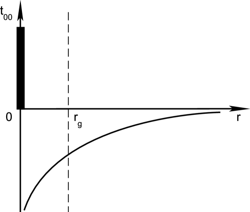
Figure 4: The energy distribution for the field configuration associated with the Schwarzschild solution. The case: $\alpha\in(0,\,2]$.

Both the gravitational potentials and the components of the total energy-momentum tensor for the field configurations with $\alpha\in[0,2]$ have no a break at $r=r_{g}$. The energy distribution is described by the $00$-component of the energy-momentum tensor, and for $\alpha\in(0,2]$ qualitatively is presented on the figure 4. Then the total energy of the system can be calculated both by the volume integration and by the surface integration over the 2-sphere with $r\rightarrow\infty$ giving $mc^{2}$. For the case $\alpha=0$ the components of the total energy-momentum tensor for the field configuration have the simplest form:

$$t^{tot}_{00} = mc^{2}\delta({\bf r})\,,$$

$$t^{tot}_{11} = -mc^{2}\delta({\bf r})\,,$$

$$t^{tot}_{AB} = -{\textstyle{1\over 2}}\overline{g}_{AB}\,mc^{2}\delta({\bf r})\,.$$ (3.88)

This energy-momentum is concentrated only at $r=0$, see the energy distribution on the figure 5. The other component $t^{tot}_{11}$ and the angular ones $t^{tot}_{AB}$ formally could be interpreted as related to the “inner” properties of the point. Indeed, they are proportional only to $\delta({\bf r})$ and, thus, describe the point “inner radial” and “inner tangent” pressure. At last, again the total energy for (3.88) is $mc^{2}$.

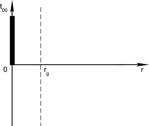
Figure 5: The energy distribution for the field configuration associated with the Schwarzschild solution. The case: $\alpha=0$.

The field configurations for $\alpha\in[0,2]$ satisfy the Einstein equations (2.65) at all the points of the Minkowski space including $r=0$. Then, keeping in mind the presentations on the figures 4 and 5 one can conclude that an appropriate description of a point particle in GR is approached. It is directly and simply continues the Newtonian derivation and, at the same time, does not contradict GR corresponding its principles.

3.6.4 Integral constraints in FRW models

In this subsection we consider the linear perturbations on FRW backgrounds from the point view of the conservation laws (3.78), or the same (3.68), for the detail calculations see [116]. Write the background metric $d\overline{s}^{2}$ in dimensionless coordinates $x^{0}=\eta,x^{k}$ as follows [153]:

$$d\overline{s}^{2}=\overline{g}_{\mu\nu}dx^{\mu}dx^{\nu}=a^{2}(\eta)(d\eta^{2}-f_{kl}dx^{k}dx^{l})=a^{2}(\eta)e_{\mu\nu}dx^{\mu}dx^{\nu},$$ (3.89)

$a(\eta)$ is the scale factor, $f_{kl}=\delta_{kl}+k{{\delta_{km}\delta_{ln}x^{m}x^{n}}}(1-kr^{2})^{-1}$, $f=det\,f_{kl}=(1-kr^{2})^{-1}$, $k=0$ or $\pm 1$, and $r^{2}=\delta_{kl}x^{k}x^{l}$. We define the perturbations by $g_{\mu\nu}=a^{2}(e_{\mu\nu}+\tilde{h}_{\mu\nu})$ as often used in cosmology (see, e.g., [126, 204]), which are connected with the the usual definition (2.13) in linear approximation:

$$\hat{l}^{\mu\nu}=a^{2}\sqrt{f}(-e^{\mu\rho}e^{\nu\sigma}+{{\textstyle{1\over 2}}}e^{\mu\nu}e^{\rho\sigma})\tilde{h}_{\rho\sigma}\,.$$ (3.90)

Because the FRW spacetimes are conformal to Minkowski space the conformal Killing vectors of FRW spacetimes are thus those of Minkowski space written in $\eta,\,x^{k}$ coordinates (see [205] - [207]). There are 15 conformal Killing vectors, ${\xi}_{A}$, $A=1,\,2,\,\ldots,\,15$, some of which are pure Killing ones.

These vectors we use as displacement vectors in the expression (3.78). Next, we make linear combinations of $\xi_{A}$’s with functions of $\eta$, say $c^{A}(\eta)\xi_{A}$. In general the $c^{A}\xi_{A}$’s are not conformal Killing vectors but some linear combinations turn out to be rather simple with clear physical interpretations in appropriate gauge conditions. Integrating the conservation law (3.78) we construct the integral relations connecting perturbations inside of a volume with perturbations at its surface. Thus we consider a sphere $r=\rm const$ at constant time $\eta$ and integrate zero components of (3.78) $\hat{J}^{0}_{(B)}=\partial_{l}\hat{J}^{0l}_{(B)}$ over such a ball. After cumbersome calculations for perturbations (3.90) one has 15 volume integrals connected with surface integrals.

Besides the matter perturbations $\delta T^{0}_{\mu}$ the volume integrands contain two field quantities ${\cal Q}=\delta(-D_{\mu}n^{\mu})$ — the perturbation of the external curvature scalar of $\eta=\rm const$, and $\tilde{h}^{m}_{m}$ — the space trace of the metric petrurbations. There are four linear combinations which do not involve $\tilde{h}^{m}_{m}$; they are associated with some linear combinations of the conformal Killing vectors, which are just Traschen’s [172] “integral constraint vectors”.

Of course, we must still impose four gauge conditions to fix the mapping of the perturbed spacetime onto the background. One gauge condition that simplifies almost all volume integrands is the “uniform Hubble expansion” gauge ${\cal Q}=0$ discussed, e.g., by Bardeen [10]. Then, 14 of the 15 volume integrands reduce to linear combinations of $\delta T^{0}_{\mu}$ only, and thus the 14 relations present “integral constraints”, among which the 4 are new. The integrals represent momenta of the matter energy-momentum tensor of order 0, 1 and 2 in powers of $x^{a}$ when $k=0$ and with similar interpretations when $k=\pm 1$. There remains one integral that contains both $\delta T^{0}_{\mu}$ and $\tilde{h}^{m}_{m}$: it is related to so-called conformal time translations for $k=\pm 1$ or to so-called time accelerations for $k=0$.

Another gauge condition often used (see, e.g., [204]) is $\nabla_{l}\vtop{{\hbox{$\tilde{h}^{l}_{k}$}} \vskip-7.0pt{\hbox{$\scriptscriptstyle T$}}}=0$ in which $\tilde{h}^{l}_{k}$ $\scriptscriptstyle T$ is the traceless part of $\tilde{h}^{l}_{k}$; these gauges remove the longitudinal modes of the gravitational waves. Combining $\nabla_{l}\vtop{{\hbox{$\tilde{h}^{l}_{k}$}} \vskip-7.0pt{\hbox{$\scriptscriptstyle T$}}}=0$ with ${\cal Q}=0$ one finds four relations that are independent of the gravitational radiation.

4 $D$-dimensional metric theories of gravity

As was discussed in Introduction, multidimensional gravitational models become more and more popular, their solutions (for example, generalized $p$-branes and brane-world black hole solutions [208] - [211]) induce an arising interest. Other generalizations, say, scalar-tensor theories of gravity [212], are developed intensively also. In this section, keeping in mind such generalizations we construct a perturbed scheme and conservation laws for perturbations in a generic metric theory. The presentation is based on the works [103, 104, 119, 121]. Besides, here the approach is presented in the united scheme, and more details are given.

4.1 The main identities

In this subsection, we present necessary identities and stress their important properties. Let the system of fields, set of tensor densities $Q^{A}$, be described by the Lagrangian

$${\hat{\cal L}}={\hat{\cal L}}(Q^{A};Q^{A}{}_{,\alpha};Q^{A}{}_{,\alpha\beta})$$ (4.1)

including derivatives up to the second order. We assume that it is an arbitrary metric theory of gravity in $D$ dimensions with the generalized gravitational variables $(g^{a},\Psi^{B})$ and the matter sources $\Phi^{C}$. Thus $Q^{A}=\{(g^{a},\Psi^{B}),\,\Phi^{C}\}$; the variables $\Psi^{B}$ are included keeping in mind, say, scalar-tensor or vector-tensor theories; the metric variables $g^{a}$ are thought as defined in (2.73), only in $D$ dimensions. Then we include $\overline{g}_{\mu\nu}$ as usual. The ordinary derivatives $\partial_{\alpha}$ are rewritten over the covariant $\overline{D}_{\alpha}$ ones by changing $Q_{B,\tau}\equiv\overline{D}_{\tau}Q_{B}-\overline{\Gamma}^{\sigma}_{\tau\rho}\left.Q_{B}\right|_{\sigma}^{\rho}$. Then the Lagrangian (4.1) takes an explicitly covariant form:

$${\hat{\cal L}}={\hat{\cal L}}_{c}={{\hat{\cal L}}}_{c}(Q_{B};\overline{D}_{\alpha}Q_{B};\overline{D}_{\beta}\overline{D}_{\alpha}Q_{B})\,.$$ (4.2)

After that indexes are shifted by $\overline{g}_{\mu\nu}$ and $\overline{g}^{\mu\nu}$.

Now we use the standard technique (see, for example, [140]). For the Lagrangian (4.2), as a scalar density, we write out again the identity: ${\pounds}_{\xi}{\hat{\cal L}}_{c}+(\xi^{\alpha}{\hat{\cal L}}_{c}){}_{,\alpha}\equiv 0$, which can be rewritten in the form:

$$-\left[{{\delta{\hat{\cal L}}_{c}}\over{\delta Q_{B}}}\overline{D}_{\alpha}Q_{B}+\overline{D}_{\beta}\left({{\delta{\hat{\cal L}}_{c}}\over{\delta Q_{B}}}\left.Q_{B}\right|^{\beta}_{\alpha}\right)\right]\xi^{\alpha}+\overline{D}_{\alpha}\left[\hat{u}^{\alpha}_{\sigma}\xi^{\sigma}+\hat{m}^{\alpha\tau}_{\sigma}\overline{D}_{\tau}\xi^{\sigma}+\hat{n}^{\alpha\tau\beta}_{\sigma}\overline{D}_{\beta}\overline{D}_{\tau}\xi^{\sigma}\right]\equiv 0\,.$$ (4.3)

In (4.3), the coefficients are defined by the Lagrangian in unique way:

$$\hat{u}^{\alpha}_{\sigma} \equiv {\hat{\cal L}}_{c}\delta^{\alpha}_{\sigma}+{{\delta{\hat{\cal L}}_{c}}\over{\delta Q_{B}}}\left.Q_{B}\right|^{\alpha}_{\sigma}-\left[{{\partial{\hat{\cal L}}_{c}}\over{\partial(\overline{D}_{\alpha}Q_{B})}}-\overline{D}_{\beta}\left({{\partial{\hat{\cal L}}_{c}}\over{\partial(\overline{D}_{\beta}\overline{D}_{\alpha}Q_{B})}}\right)\right]\overline{D}_{\sigma}Q_{B}$$ (4.4)

$$- {{\partial{\hat{\cal L}}_{c}}\over{\partial(\overline{D}_{\beta}\overline{D}_{\alpha}Q_{B})}}\overline{D}_{\sigma}\overline{D}_{\beta}Q_{B}-\hat{n}^{\alpha\tau\beta}_{\lambda}\overline{R}^{\lambda}_{~{}\tau\beta\sigma}\,,$$

$$\hat{m}^{\alpha\tau}_{\sigma} \equiv \left[{{\partial{\hat{\cal L}}_{c}}\over{\partial(\overline{D}_{\alpha}Q_{B})}}-\overline{D}_{\beta}\left({{\partial{\hat{\cal L}}_{c}}\over{\partial(\overline{D}_{\beta}\overline{D}_{\alpha}Q_{B})}}\right)\right]\left.Q_{B}\right|^{\tau}_{\sigma}$$ (4.5)

$$- {{\partial{\hat{\cal L}}_{c}}\over{\partial(\overline{D}_{\tau}\overline{D}_{\alpha}Q_{B})}}\overline{D}_{\sigma}Q_{B}+{{\partial{\hat{\cal L}}_{c}}\over{\partial(\overline{D}_{\beta}\overline{D}_{\alpha}Q_{B})}}\overline{D}_{\beta}(\left.Q_{B}\right|^{\tau}_{\sigma})\,,$$

$$\hat{n}^{\alpha\tau\beta}_{\sigma}\equiv{\textstyle{1\over 2}}\left[{{\partial{\hat{\cal L}}_{c}}\over{\partial(\overline{D}_{\beta}\overline{D}_{\alpha}Q_{B})}}\left.Q_{B}\right|^{\tau}_{\sigma}+{{\partial{\hat{\cal L}}_{c}}\over{\partial(\overline{D}_{\tau}\overline{D}_{\alpha}Q_{B})}}\left.Q_{B}\right|^{\beta}_{\sigma}\right].$$ (4.6)

The coefficient at $\xi^{\sigma}$ in the first term in (4.3) is identically equal to zero (generalized Bianchi identity). Thus the identity (4.3) has the form of the differential conservation law:

$$\overline{D}_{\alpha}\hat{\imath}^{\alpha}\equiv\partial_{\alpha}\hat{\imath}^{\alpha}\equiv 0$$ (4.7)

with a generalized current

$$\hat{\imath}^{\alpha}\equiv-\left[\hat{u}^{\alpha}_{\sigma}\xi^{\sigma}+\hat{m}^{\alpha\tau}_{\sigma}\overline{D}_{\tau}\xi^{\sigma}+\hat{n}^{\alpha\tau\beta}_{\sigma}\overline{D}_{\beta}\overline{D}_{\tau}\xi^{\sigma}\right]\,.$$ (4.8)

We also use the helpful form:

$$\hat{\imath}^{\alpha}\equiv-\left[(\hat{u}^{\alpha}_{\sigma}+\hat{n}^{\alpha\beta\gamma}_{\lambda}\overline{R}^{\lambda}_{~{}\beta\gamma\sigma})\xi^{\sigma}+\hat{m}^{\alpha\beta}_{\sigma}\bar{g}^{\sigma\rho}\partial_{[\beta}\xi_{\rho]}+\hat{z}^{\alpha}\right]$$ (4.9)

with $z$-term defined as

$$\hat{z}^{\alpha}(\xi)\equiv\hat{m}^{\alpha\beta}_{\sigma}\zeta^{\sigma}_{\beta}+\hat{n}^{\alpha\beta\gamma}_{\sigma}\overline{g}^{\sigma\rho}\left(2\overline{D}_{\gamma}\zeta_{\beta\rho}-\overline{D}_{\rho}\zeta_{\beta\gamma}\right)\,.$$ (4.10)

Again, if $\xi^{\alpha}=\lambda^{\alpha}$, then $\hat{z}^{\alpha}=0$ and the current (4.9) is determined by the energy-momentum $(u+n\overline{R})$-term and the spin $m$-term. Opening the identity (4.7) and, since $\xi^{\sigma}$, $\partial_{\alpha}\xi^{\sigma}$, $\partial_{\beta\alpha}\xi^{\sigma}$ and $\partial_{\gamma\beta\alpha}\xi^{\sigma}$ are arbitrary at every world point, equating independently to zero the coefficients at $\xi^{\sigma}$, $\overline{D}_{\alpha}\xi^{\sigma}$, $\overline{D}_{(\beta\alpha)}\xi^{\sigma}$ and $\overline{D}_{(\gamma\beta\alpha)}\xi^{\sigma}$ we get a “cascade” (in terminology by Julia and Silva [183]) of identities:

$$\overline{D}_{\alpha}\hat{u}^{\alpha}_{\sigma}+{\textstyle{1\over 2}}\hat{m}^{\alpha\rho}_{\lambda}\overline{R}^{~{}\lambda}_{\sigma~{}\rho\alpha}+{\textstyle{1\over 3}}\hat{n}^{\alpha\rho\gamma}_{\lambda}\overline{D}_{\gamma}\overline{R}^{~{}\lambda}_{\sigma~{}\rho\alpha}\equiv 0,$$

$$\hat{u}^{\alpha}_{\sigma}+\overline{D}_{\lambda}\hat{m}^{\lambda\alpha}_{\sigma}+\hat{n}^{\tau\alpha\rho}_{\lambda}\overline{R}^{~{}\lambda}_{\sigma~{}\rho\tau}+{\textstyle{2\over 3}}\hat{n}^{\lambda\tau\rho}_{\sigma}\overline{R}^{\alpha}_{~{}\tau\rho\lambda}\equiv 0,$$

$$\hat{m}^{(\alpha\beta)}_{\sigma}+\overline{D}_{\lambda}\hat{n}^{\lambda(\alpha\beta)}_{\sigma}\equiv 0,$$

$$\hat{n}^{(\alpha\beta\gamma)}_{\sigma}\equiv 0.$$ (4.11)

The above constructions are the generalization to arbitrary curved backgrounds of the expressions given by Mitzkevich [140].

Since Eq. (4.7) is identically satisfied, the current (4.9) must be a divergence of a superpotential $\hat{\imath}^{\alpha\beta}$, for which $\partial_{\beta\alpha}\hat{\imath}^{\alpha\beta}\equiv 0$, that is

$$\hat{\imath}^{\alpha}\equiv\overline{D}_{\beta}\hat{\imath}^{\alpha\beta}\equiv\partial_{\beta}\hat{\imath}^{\alpha\beta}.$$ (4.12)

Indeed, substituting $\hat{u}^{\alpha}_{\sigma}$ and $\hat{m}^{\alpha\beta}_{\sigma}$ from Eqs. (4.11) directly into the current and using algebraic properties of $n^{\alpha\beta\gamma}_{\sigma}$ and $\overline{R}^{\alpha}_{~{}\beta\rho\sigma}$, and the third identity in Eqs. (4.11) we reconstruct (4.9) into the form (4.12) where the superpotential is

$$\hat{\imath}^{\alpha\beta}\equiv\left({\textstyle{2\over 3}}\overline{D}_{\lambda}\hat{n}^{[\alpha\beta]\lambda}_{\sigma}-\hat{m}^{[\alpha\beta]}_{\sigma}\right)\xi^{\sigma}-{\textstyle{4\over 3}}\hat{n}^{[\alpha\beta]\lambda}_{\sigma}\overline{D}_{\lambda}\xi^{\sigma}.$$ (4.13)

It is explicitly antisymmetric in $\alpha$ and $\beta$. Of course, Eq. (4.12) has also a sense of the differential conservation law Eq. (4.7).

Let us find contributions into currents and superpotentials from a divergence in the Lagrangian $\delta_{d}{\hat{\cal L}}_{c}=div=\hat{d}^{\nu}{}_{,\nu}$. For the scalar density $\hat{d}^{\nu}{}_{,\nu}$ one has the identity $({\pounds_{\xi}}\hat{d}^{\alpha}+\xi^{\alpha}\hat{d}^{\nu}{}_{,\nu})_{,\alpha}\equiv 0$, which gives contributions $\delta_{d}\hat{\imath}^{\alpha}$ into the current (4.8) and $\delta_{d}\hat{\imath}^{\alpha\beta}$ into the superpotential (4.13). The additional quantities are

$$\delta_{d}\hat{u}^{\alpha}_{\sigma} = 2\overline{D}_{\beta}(\delta^{[\alpha}_{\sigma}\hat{d}^{\beta]})\,,$$ (4.14)

$$\delta_{d}\hat{m}^{\alpha\beta}_{\sigma} = 2\delta^{[\alpha}_{\sigma}\hat{d}^{\beta]}\,,$$ (4.15)

$$\delta_{d}\hat{n}^{\alpha\beta\gamma}_{\sigma} = 0\,,$$ (4.16)

$$\delta_{d}\hat{\imath}^{\alpha\beta} = -2\xi^{[\alpha}\hat{d}^{\beta]}\,.$$ (4.17)

Then, for ${\hat{\cal L}}_{c}\rightarrow{\hat{\cal L}}_{c}+\delta_{d}{\hat{\cal L}}_{c}$ Eq. (4.12) changes as

$$\hat{\imath}^{\alpha}+\delta_{d}\hat{\imath}^{\alpha}\equiv\overline{D}_{\beta}\left(\hat{\imath}^{\alpha\beta}+\delta_{d}\hat{\imath}^{\alpha\beta}\right),$$ (4.18)

where the changes do not depend on a structure of $\hat{d}^{\nu}$.

Next, using the general Belinfante rule (3.27) we define a tensor density

$$\hat{s}^{\alpha\beta\sigma}\equiv-\hat{s}^{\beta\alpha\sigma}\equiv-\hat{m}^{\sigma[\alpha}_{\lambda}\bar{g}^{\beta]\lambda}-\hat{m}^{\alpha[\sigma}_{\lambda}\bar{g}^{\beta]\lambda}+\hat{m}^{\beta[\sigma}_{\lambda}\bar{g}^{\alpha]\lambda}\,,$$ (4.19)

add $\overline{D}_{\beta}(\hat{s}^{\alpha\beta\sigma}\xi_{\sigma})$ to both sides of (4.12), and obtain a new identity:

$$\hat{\imath}^{\alpha}_{B}\equiv\overline{D}_{\beta}\hat{\imath}^{\alpha\beta}_{B}\equiv\partial_{\beta}\hat{\imath}^{\alpha\beta}_{B}.$$ (4.20)

This modification cancels the spin term from the current (4.9):

$$\hat{\imath}^{\alpha}_{B}\equiv\left(-\hat{u}^{\alpha}_{\sigma}-\hat{n}^{\alpha\beta\gamma}_{\lambda}\overline{R}^{\lambda}_{~{}\beta\gamma\sigma}+\overline{D}_{\beta}\hat{s}^{\alpha\beta}{}_{\sigma}\right)\xi^{\sigma}+\hat{z}^{\alpha}_{B}(\xi)\equiv\hat{u}_{B\sigma}^{\alpha}\xi^{\sigma}+\hat{z}^{\alpha}_{B}(\xi),$$ (4.21)

and a new $z$-term disappears also on Killing vectors of the background:

$$\hat{z}^{\alpha}_{B}(\xi)=\left(\bar{g}^{\lambda\tau}\hat{m}^{\beta\alpha}_{\lambda}+\hat{m}^{\alpha\tau}_{\lambda}\bar{g}^{\beta\lambda}-\hat{m}^{\tau\beta}_{\lambda}\bar{g}^{\alpha\lambda}\right)\zeta_{\tau\beta}+\hat{n}^{\alpha\tau\beta}_{\lambda}\left(2\overline{D}_{(\beta}\zeta_{\tau)}^{\lambda}-\overline{D}_{\sigma}\zeta_{\beta\tau}\bar{g}^{\lambda\sigma}\right)\,.$$ (4.22)

Thus, the current $\hat{i}^{\alpha}_{B}$ is defined, in fact, by the modified energy-momentum tensor density $\hat{u}_{B\sigma}^{\alpha}$. Because the new superpotential depends on the $n$-coefficients only:

$$\hat{i}^{\alpha\beta}_{B}\equiv 2\left({\textstyle{1\over 3}}\overline{D}_{\rho}\hat{n}^{[\alpha\beta]\rho}_{\sigma}+\overline{D}_{\tau}\hat{n}^{\tau\rho[\alpha}_{\lambda}\bar{g}^{\beta]\lambda}\bar{g}_{\rho\sigma}\right)\xi^{\sigma}-{\textstyle{4\over 3}}\hat{n}^{[\alpha\beta]\lambda}_{\sigma}\overline{D}_{\lambda}\xi^{\sigma},$$ (4.23)

then due to the definition (4.6) it vanishes for Lagrangians with only the first order derivatives. On the other hand, the superpotential (4.23) is well adapted to theories with second derivatives in Lagrangians, like GR or the Einstein-Gauss-Bonnet gravity. It is also important to note that for the superpotentials (4.13) and (4.23) their forms do not depend explicitly on a dimension $D$; the same property is related to the Deser and Tekin superpotentials [75].

It is important to note that the Belinfante procedure applied to (4.18) cancels the quantities $\delta_{d}\hat{\imath}^{\alpha}$ and $\delta_{d}\hat{\imath}^{\alpha\beta}$ and gives again (4.20). Let us show this. The quantity (4.19) constructed for $\delta_{d}\hat{m}^{\alpha\beta}_{\sigma}$ in (4.15) gives

$$\delta_{d}\hat{s}^{\alpha\beta\sigma}\xi_{\sigma}=2\xi^{[\alpha}\hat{d}^{\beta]}\,.$$ (4.24)

Then, adding $\overline{D}_{\beta}(\hat{s}^{\alpha\beta\sigma}\xi_{\sigma}+\delta_{d}\hat{s}^{\alpha\beta\sigma}\xi_{\sigma})$ to Eq. (4.18) one cancels completely the spin term and suppresses $\delta_{d}\hat{u}^{\alpha}_{\sigma}$ and $\delta_{d}\hat{\imath}^{\alpha\beta}$. Indeed, combining (4.14) and (4.17) with (4.24) one has $\delta_{d}\hat{u}^{\alpha}_{\sigma}-\overline{D}_{\beta}(\delta_{d}\hat{s}^{\alpha\beta\rho}\bar{g}_{\rho\sigma})=0$ and  $\delta_{d}\hat{\imath}^{\alpha\beta}+\delta_{d}\hat{s}^{\alpha\beta\sigma}\xi_{\sigma}=0$ for an arbitrary $\hat{d}^{\nu}$. This just supports the claim that $\hat{J}^{\mu}_{(B)}$, $\hat{\Theta}^{\mu}{}_{(B)\nu}$ and $\hat{J}^{\mu\nu}_{(B)}$ in (3.78) are independent on divergences.

4.2 The field-theoretical formulation for perturbations

In this subsection, following the method of section 2 we develop a perturbed derivation. The field equations corresponding to the system (4.1) are derived as usual:

$${\delta{\hat{\cal L}}}/{\delta Q^{A}}=0\,.$$ (4.25)

Let us decompose $Q^{A}$ onto the background part $\overline{Q}^{A}$ and the dynamic part $q^{A}$:

$$Q^{A}=\overline{Q}^{A}+q^{A}\,.$$ (4.26)

The background fields satisfy the background equations

$${\delta\overline{\hat{\cal L}}}/{\delta\overline{Q}^{A}}=0\,$$ (4.27)

where $\overline{\hat{\cal L}}={\hat{\cal L}}(\overline{Q})$. Taking into account the form of the Lagrangian (2.19) (or (2.77)) we will describe the perturbed system by the Lagrangian

$${\hat{\cal L}}^{dyn}(\overline{Q},q)={\hat{\cal L}}(\overline{Q}+q)-q^{A}\frac{\delta\overline{\hat{\cal L}}}{\delta\overline{Q}^{A}}-\overline{\hat{\cal L}}+div$$ (4.28)

instead of the original Lagrangian ${\hat{\cal L}}(Q)={\hat{\cal L}}(\overline{Q}+q)$. As before, the background equations should not be taken into account before variation of ${\hat{\cal L}}^{dyn}(\overline{Q},q)$ with respect to $\overline{Q}^{A}$. Using the evident property ${\delta{\hat{\cal L}}(\overline{Q}+q)}/{\delta\overline{Q}^{A}}={\delta{\hat{\cal L}}(\overline{Q}+q)}/{\delta q^{A}}$, the equations of motion related to the Lagrangian (4.28) are presented as

$$\frac{\delta{\hat{\cal L}}^{dyn}}{\delta q^{A}}=\frac{\delta}{\delta\overline{Q}^{A}}\left[{\hat{\cal L}}(\overline{Q}+q)-\overline{\hat{\cal L}}\right]=0\,.$$ (4.29)

It is clear that they are equivalent to the equations (4.25) if the background equations (4.27) hold.

Defining the “background current”

$$t^{q}_{A}\equiv\frac{\delta{\hat{\cal L}}^{dyn}}{\delta\overline{Q}^{A}}=\frac{\delta{\hat{\cal L}}^{dyn}}{\delta q^{A}}-\frac{\delta}{\delta\overline{Q}^{A}}q^{B}\frac{\delta\overline{\hat{\cal L}}}{\delta\overline{Q}^{B}}\,$$ (4.30)

and combining this expression with (4.29) one obtains another form for the equation (4.29):

$$G^{Lq}_{A}+\Phi^{Lq}_{A}\equiv-\frac{\delta}{\delta\overline{Q}^{A}}q^{B}\frac{\delta\overline{\hat{\cal L}}}{\delta\overline{Q}^{B}}=t^{q}_{A}\,.$$ (4.31)

The left hand side in (4.31) is a linear perturbation of the expression ${\delta{\hat{\cal L}}}/{\delta Q^{A}}$ in (4.25), $G^{L}_{A}$ is a pure gravitational part. Really gravitational variables $g^{a}$ and $\Psi^{B}$ have a different nature. Conservation laws are connected with symmetries of a geometry related directly to $g^{a}$, not with $\Psi^{B}$. Thus, we will consider $\Psi^{B}$ as included in $\Phi^{B}$, setting thus in calculations $\Psi^{B}=0$ and $Q^{A}=\{g^{a},\,\Phi^{B}\}$. Later we will consider the lagrangian

$${\hat{\cal L}}={\hat{\cal L}}_{Dg}(g^{a})+{\hat{\cal L}}_{Dm}(g^{a},\Phi^{B})$$ (4.32)

with the pure metric gravitational part ${\hat{\cal L}}_{Dg}$. Then the equations (4.30) are separated into gravitational and matter parts as follows

$$G^{Lq}_{a}+\Phi^{Lq}_{a}\equiv-\frac{\delta}{\delta\overline{g}^{a}}q^{B}\frac{\delta\overline{{\hat{\cal L}}}}{\delta\overline{Q}^{B}}=t^{q}_{a}\,,$$ (4.33)

$$\Phi^{Lq}_{C}\equiv-\frac{\delta}{\delta\overline{\Phi}^{C}}q^{B}\frac{\delta\overline{{\hat{\cal L}}}_{Dm}}{\delta\overline{Q}^{B}}=t^{q}_{C}\,.$$ (4.34)

As is seen, the form of the perturbed equations (4.31), (4.33) and (4.34) is a quite universal form with the “background current” as a source on the right hand side. Contracting (4.33) with $2\partial\overline{g}^{a}/\overline{g}^{\mu\nu}$ one obtains

$$\hat{G}^{Lq}_{\mu\nu}+\hat{\Phi}^{Lq}_{\mu\nu}=\hat{t}^{q}_{\mu\nu}\,$$ (4.35)

where the linear operator is defined as

$$\hat{G}^{Lq}_{\mu\nu}+\hat{\Phi}^{Lq}_{\mu\nu}\equiv-2\frac{\delta}{\delta\overline{g}^{\mu\nu}}\left(\hat{l}^{\alpha\beta}_{(a)}\frac{\delta\overline{\hat{\cal L}}_{Dg}}{\delta\overline{\hat{g}}^{\alpha\beta}}+q^{B}\frac{\delta\overline{\hat{\cal L}}_{Dm}}{\delta\overline{Q}^{B}}\right)$$ (4.36)

with independent gravitational variables $\hat{l}^{\alpha\beta}_{(a)}$ defined as in (2.80). The right hand side in (4.35) is defined by variation of (4.28)

$$\hat{t}^{q}_{\mu\nu}\equiv 2\frac{\delta{\hat{\cal L}}^{dyn}(\overline{Q},q)}{\delta\overline{g}^{\mu\nu}}$$ (4.37)

and is the generalized symmetric energy-momentum.

The equations (4.35) generalize the equations of GR (2.23), they generalize also the Deser-Tekin equations [75, 213, 214] constructed for the quadratic theories by direct calculations. Below we will show that for the vacuum backgrounds (when $\hat{\Phi}^{Lq}_{\mu\nu}=0$) $\overline{D}^{\mu}\hat{G}^{Lq}_{\mu\nu}\equiv 0$, and thus the energy momentum tensor $\hat{t}^{q}_{\mu\nu}$ is differentially conserved, like in the Petrov spaces (2.66) in GR. The presented here model has the same properties for expansions as was described in subsection 2.5 and the same gauge properties as was described in detail in subsection 2.6.

4.3 Currents and superpotentials in the field formulation

In the recent series of the current works [75, 76, 213, 214] Deser with coauthors develop a construction of conserved charges for perturbations about vacua in metric quadratic (in curvature) gravity theories in $D$ dimensions. They apply the Abbott and Deser procedure [68] and develop it. The aim of the present subsection is to suggest an approach, which generalizes the Deser and Tekin constructions. We construct conserved currents and superpotentials corresponding to the equations (4.35) derived for an arbitrary metrical gravitational theory, and not only on a vacuum background. Below taking into account the definition of the gravitational part of linear operator (4.36) we demonstrate that conserved quantities of the system and their properties can be obtained and described analyzing only the scalar density ${\hat{\cal L}}_{1}\equiv\hat{l}_{(a)}^{\alpha\beta}({\delta\overline{\hat{\cal L}}_{Dg}}/{\delta\overline{\hat{g}}^{\alpha\beta}})$, which is the gravitational part of second term in the Lagrangian (4.28). As an important case we consider explicitly only such theories where ${\hat{\cal L}}_{1}$ has derivatives not higher than of second order, like the Einstein-Gauss-Bonnet gravity. In principle, our results can be repeated when ${\hat{\cal L}}_{1}$ has derivatives of higher orders, like in [75].

Keeping in mind that ${\hat{\cal L}}_{1}$ is the scalar density we again follow the standard technique and use the results of the subsection 4.1, which are universal. One transforms the identity ${\pounds}_{\xi}{\hat{\cal L}}_{1}+\partial_{\alpha}(\xi^{\alpha}{\hat{\cal L}}_{1})\equiv 0$ into the identity:

$$\overline{D}_{\mu}\hat{\imath}_{1}^{\mu}\equiv\partial_{\mu}\hat{\imath}_{1}^{\mu}\equiv 0\,$$ (4.38)

where

$$\hat{\imath}_{1}^{\mu} \equiv -\left({\hat{\cal L}}_{1}\xi^{\mu}+\xi^{\nu}\left.\hat{l}^{\rho\sigma}_{(a)}\right|^{\mu}_{\nu}\frac{\delta\overline{\hat{\cal L}}_{Dg}}{\delta\overline{\hat{g}}^{\rho\sigma}}+2\xi^{\sigma}\frac{\delta{\hat{\cal L}}_{1}}{\delta\overline{g}^{\rho\sigma}}\overline{g}^{\rho\mu}\right)+\hat{\cal Z}^{\mu}_{(s)}\,,$$ (4.39)

$$\hat{\cal Z}^{\mu}_{(s)} \equiv 2\frac{\partial{\hat{\cal L}}_{1}}{\partial\overline{g}_{\rho\sigma,\mu\nu}}\overline{D}_{\nu}\zeta_{\rho\sigma}-2\zeta_{\rho\sigma}\overline{D}_{\nu}\frac{\partial{\hat{\cal L}}_{1}}{\partial\overline{g}_{\rho\sigma,\mu\nu}}\,.$$ (4.40)

It is just the current (4.8) for the Lagrangian ${\hat{\cal L}}_{1}$.

In the case of a vacuum background one has ${\delta\overline{\hat{\cal L}}_{Dg}}/{\delta\overline{\hat{g}}^{\rho\sigma}}=0$ and ${\hat{\cal L}}_{1}=0$. Then assuming arbitrary Killing vectors $\xi^{\alpha}=\lambda^{\alpha}$ one transforms the identity (4.38) into

$$\overline{D}_{\mu}\left(\frac{\delta{\hat{\cal L}}_{1}}{\delta\overline{g}_{\mu\nu}}\right)\equiv\overline{D}_{\mu}\left(\frac{\delta}{\delta\overline{g}_{\mu\nu}}\hat{l}^{\alpha\beta}_{(a)}\frac{\delta\overline{\hat{\cal L}}_{Dg}}{\delta\overline{\hat{g}}^{\alpha\beta}}\right)\equiv 0\,.$$ (4.41)

Recalling that for the vacuum case $\hat{\Phi}^{Lq}_{\mu\nu}=0$ and taking into account the identity (4.41) with the definition (4.36) in the equations (4.35) one gets $\overline{D}_{\mu}\hat{t}_{q}^{\mu\nu}=0$. This generalizes the results in [213, 75] for the quadratic theories. Recall also that in the Lagrangian (2.68) $\Lambda$-term was interpreted as “degenerated” matter, then with this assumption the identity (2.71) has been approached. However, the Lagrangian (2.68) fully is, of course, a kind of metric Lagrangians, therefore the identity (2.71) also is interpreted in the terms of the general formula (4.41).

Again, because (4.38) is the identity the current $\hat{\imath}^{\mu}_{1}$ has to be presented through a divergence of a superpotential. To construct the last we use the results of the subsection 4.1 adopted for the Lagrangian ${\hat{\cal L}}_{1}$. We set $\overline{g}_{\mu\nu}\rightarrow g_{\mu\nu}$ and construct the coefficients (4.5) - (4.6) with ${\hat{\cal L}}_{1}={\hat{\cal L}}_{1}(Q;\,\partial_{\mu}Q;\,\partial_{\mu\nu}Q)\equiv{\hat{\cal L}}_{1}^{c}(Q;\,\overline{D}_{\mu}Q;\,\overline{D}_{\mu\nu}Q)$, where $Q^{A}=\{\hat{l}_{a}^{\mu\nu},\,g_{\mu\nu}\}$. Then we go back, $g_{\mu\nu}\rightarrow\overline{g}_{\mu\nu}$, and obtain simple expressions

$$\hat{m}_{1\sigma}{}^{\mu\nu}=2\overline{D}_{\lambda}\left(\frac{\partial{\hat{\cal L}}_{1}}{\partial\overline{g}_{\rho\nu,\mu\lambda}}\right)\overline{g}_{\rho\sigma}\,,\qquad\hat{n}_{1\sigma}^{\lambda\mu\nu}=-2\frac{\partial{\hat{\cal L}}_{1}}{\partial\overline{g}_{\rho(\mu,\nu)\lambda}}\overline{g}_{\rho\sigma}\,.$$ (4.42)

Then, substituting these into the expression (4.13) we can define the superpotential $\hat{\cal I}_{(s)}^{\mu\nu}$, which is evidently linear in $\hat{l}_{(a)}^{\mu\nu}$. In the case of the Einstein gravity it is the superpotential (3.74). Thus, we have the identity

$$\hat{\imath}^{\mu}_{1}\equiv\partial_{\nu}\hat{\cal I}_{(s)}^{\mu\nu}\,,$$ (4.43)

which generalizes the identity (3.72) and the superpotential has the form:

$$\hat{\cal I}_{(s)}^{\alpha\beta}\equiv\left({\textstyle{2\over 3}}\overline{D}_{\lambda}\hat{n}^{[\alpha\beta]\lambda}_{1\sigma}-\hat{m}^{[\alpha\beta]}_{1\sigma}\right)\xi^{\sigma}-{\textstyle{4\over 3}}\hat{n}^{[\alpha\beta]\lambda}_{1\sigma}\overline{D}_{\lambda}\xi^{\sigma}.$$ (4.44)

Using in (4.39) the field equations in the form (4.35) and the definition (4.36) we write out the physically real current: $\hat{\imath}_{1}^{\mu}\rightarrow\hat{\cal I}_{(s)}^{\mu}$:

$$\hat{\cal I}_{(s)}^{\mu}\equiv\hat{\cal T}^{\mu}_{(s)\nu}\xi^{\nu}+\hat{\cal Z}^{\mu}_{(s)}\,$$ (4.45)

where the generalized energy-momentum is

$$\hat{\cal T}^{\mu}_{(s)\nu}\equiv\left(\hat{t}_{q\nu}^{\mu}-\hat{\Phi}_{Lq\nu}^{\mu}\right)-\left(\delta^{\mu}_{\nu}\hat{l}^{\rho\sigma}_{(a)}\frac{\delta\overline{\hat{\cal L}}_{Dg}}{\delta\overline{\hat{g}}^{\rho\sigma}}+\left.\hat{l}^{\rho\sigma}_{(a)}\right|^{\mu}_{\nu}\frac{\delta\overline{\hat{\cal L}}_{Dg}}{\delta\overline{\hat{g}}^{\rho\sigma}}\right)\,.$$ (4.46)

Thus finally the identity (4.43) transforms to the conservation law:

$$\hat{\cal I}^{\mu}_{(s)}=\partial_{\nu}\hat{\cal I}_{(s)}^{\mu\nu}\,.$$ (4.47)

The expressions (4.45) and (4.46) are based on the symmetrical energy-momentum (4.37) and generalize the correspondent expressions in GR: (3.68) and (3.69), therefore we choose the subscript “$(s)$”. Thus, this subsection, generalizing the results of the subsection 3.4 develop the idea to use the identity (3.67) in GR. The expression (4.47), on the one hand, generalizes the conservation law (3.73) in GR, on the other hand, it generalizes the Deser-Tekin expressions [75, 213, 214]. In the case of a vacuum background and using the Killing vectors $\xi^{\alpha}=\lambda^{\alpha}$ one has for the current

$$\hat{\cal I}_{(s)}^{\mu}=\hat{t}_{q\nu}^{\mu}\lambda^{\nu}\,,$$ (4.48)

that also is in correspondence with the general definition (3.23) in a field theory.

4.4 Canonical Nœther and Belinfante symmetrized currents and
superpotentials

The expressions presented in subsection 4.1 are maximally adopted to construct both Noether canonical conserved quantities in the framework of the bimetric formulation and Belinfante corrected quantities. To construct such quantities one has to consider a pure metric part ${\hat{\cal L}}_{Dg}$ of the Lagrangian (4.32). At the beginning we construct the Nœther canonical quantities. We construct the corresponding to ${\hat{\cal L}}_{Dg}$ coefficients (4.4) - (4.6), $\hat{u}^{\alpha}_{g\sigma}$, $\hat{m}^{\alpha\beta}_{g\sigma}$, $\hat{n}^{\alpha\beta\gamma}_{g\sigma}$, with the use of which we present the related identity (4.12):

$$\hat{\imath}^{\alpha}_{g}\equiv\partial_{\beta}\hat{\imath}^{\alpha\beta}_{g}\,.$$ (4.49)

Next, following to the KBL ideology (3.41) we construct a metric Lagrangian for the perturbed system:

$${\hat{\cal L}}_{DG}={\hat{\cal L}}_{Dg}-\overline{\hat{\cal L}}_{Dg}+\partial_{\alpha}\hat{d}^{\alpha}\,.$$ (4.50)

Then, we apply the barred procedure to the identity (4.49) and take into account the divergence keeping in mind (4.14) - (4.18). As a result we obtain the identity corresponding to (4.50):

$$\hat{\imath}^{\alpha}_{g}-\overline{\hat{\imath}^{\alpha}_{g}}+\delta_{d}\hat{\imath}^{\alpha}_{g}\equiv\overline{D}_{\beta}\left[\hat{\imath}_{g}^{\alpha\beta}(\xi)-\overline{\hat{\imath}^{\alpha\beta}_{g}}(\xi)+\delta_{d}{\hat{\imath}}^{\alpha\beta}_{g}(\xi)\right]\,.$$ (4.51)

After substituting the dynamical equations (4.25) and the background equations (4.27) in the form

$$\frac{\delta{\hat{\cal L}}_{Dg}}{\delta g^{a}} = -\frac{\delta{\hat{\cal L}}_{Dm}}{\delta g^{a}}\,,$$ (4.52)

$$\frac{\delta\overline{\hat{\cal L}}_{Dg}}{\delta\overline{g}^{a}} = -\frac{\delta\overline{\hat{\cal L}}_{Dm}}{\delta\overline{g}^{a}}$$ (4.53)

into $\hat{u}^{\alpha}_{g\sigma}$ and $\overline{\hat{u}}^{\alpha}_{g\sigma}$ one obtains $\hat{U}^{\alpha}_{g\sigma}$ and $\overline{\hat{U}}^{\alpha}_{g\sigma}$, respectively. Then the identity (4.51) transforms into a real conservation law:

$$\hat{\cal I}^{\alpha}_{(c)}(\xi)=\partial_{\beta}\hat{\cal I}^{\alpha\beta}_{(c)}(\xi)\,.$$ (4.54)

The left hand side (current), in correspondence with (4.9), is

$$\hat{\cal I}^{\alpha}_{(c)}(\xi)\equiv\hat{\cal T}^{\alpha}_{\sigma(c)}\xi^{\sigma}+\hat{\cal S}^{\alpha\beta\rho}_{(c)}\partial_{[\beta}\xi_{\rho]}+\hat{\cal Z}^{\alpha}_{(c)}(\xi)$$ (4.55)

where the generalized canonical energy-momentum, spin and $Z$-term are

$$\hat{\cal T}^{\alpha}_{\sigma(c)} \equiv -\left[\left(\delta\hat{U}^{\alpha}_{g\sigma}+2\overline{D}_{\beta}(\delta^{[\alpha}_{\sigma}\hat{d}^{\beta]})\right)+\delta\hat{n}^{\alpha\beta\gamma}_{g\lambda}\overline{R}^{\lambda}_{~{}\beta\gamma\sigma}\right]$$ (4.56)

$$\hat{\cal S}^{\alpha\rho\beta}_{(c)} \equiv \delta\hat{m}^{\alpha\beta}_{g\sigma}+2\delta^{[\alpha}_{\sigma}\hat{d}^{\beta]}\bar{g}^{\sigma\rho}$$ (4.57)

$$\hat{\cal Z}^{\alpha}_{(c)}(\xi) \equiv -\left(\delta\hat{z}^{\alpha}_{g}+2\delta^{[\alpha}_{\sigma}\hat{d}^{\beta]}\zeta^{\sigma}_{\beta}\right)\,.$$ (4.58)

A more detailed expression for the superpotential is

$$\hat{\cal I}^{\alpha\beta}_{(c)}(\xi) \equiv \hat{\imath}_{g}^{\alpha\beta}(\xi)-\overline{\hat{\imath}^{\alpha\beta}_{g}}(\xi)+\delta_{d}\hat{\imath}_{g}^{\alpha\beta}(\xi)$$ (4.59)

$$= \left({\textstyle{2\over 3}}\overline{D}_{\lambda}\delta\hat{n}^{[\alpha\beta]\lambda}_{\sigma}-\delta\hat{m}^{[\alpha\beta]}_{\sigma}\right)\xi^{\sigma}-{\textstyle{4\over 3}}\delta\hat{n}^{[\alpha\beta]\lambda}_{g\sigma}\overline{D}_{\lambda}\xi^{\sigma}-2\xi^{[\alpha}\hat{d}^{\beta]}\,.$$

Here the perturbed expressions are used:

$$\delta\hat{U}^{\alpha}_{g\sigma} = \hat{U}^{\alpha}_{g\sigma}-\overline{\hat{U}}^{\alpha}_{g\sigma}\,,$$ (4.60)

$$\delta\hat{m}^{\alpha\beta}_{g\sigma} = \hat{m}^{\alpha\beta}_{g\sigma}-\overline{\hat{m}}^{\alpha\beta}_{g\sigma}\,,$$ (4.61)

$$\delta\hat{n}^{\lambda\alpha\beta}_{g\sigma} = \hat{n}^{\lambda\alpha\beta}_{g\sigma}-\overline{\hat{n}}^{\lambda\alpha\beta}_{g\sigma}\,.$$ (4.62)

The perturbation $\delta\hat{z}^{\alpha}_{g}$ is defined by the the definition (4.10) and by the perturbations (4.61) and (4.62). Of course, if a displacement vector is a Killing vector in the background spacetime then $\hat{\cal Z}^{\alpha}_{(c)}$ disappears. In the case of GR the conservation law (4.54) goes to the KBL conservation law (3.55), if $\hat{d}^{\alpha}$ is defined as $\hat{k}^{\alpha}$ in (2.20).

The presented here procedure gives well defined currents and superpotentials in the following sense. Without changing the identity (4.7) one can add to the current an arbitrary quantity $\Delta\hat{\imath}^{\alpha}(\xi)$ satisfying $[\Delta\hat{\imath}^{\alpha}(\xi)]_{,\alpha}\equiv 0$. Analogously, without changing $\hat{\imath}^{\alpha}$ in (4.12) the superpotential can be added by $\Delta\hat{\imath}^{\alpha\beta}(\xi)$ with the property $[\Delta\hat{\imath}^{\alpha\beta}(\xi)]_{,\beta}\equiv 0$. However, the “broken” current and superpotential can be “restored” by the same way because the quantities $\Delta\hat{\imath}^{\alpha}(\xi)$ and $\Delta\hat{\imath}^{\alpha\beta}(\xi)$ are not connected at all with the procedure applied to the given Lagrangian in a non-explicit form. Whereas, in the sense of the procedure, the current and the superpotential in Eq. (4.12) are given by the coefficients (4.4) - (4.6) uniquely defined by the Lagrangian. This claim develops also the criteria by Szabados [168] who suggested to consider a connection of pseudotensors with Lagrangians “as a selection rule to choose from the mathematically possible pseudotensors”. Thus one can assert that the current and superpotential in (4.54) are defined by the unique way in the above sense. Of course, the same claim is related to the KBL quantities in (3.55). They uniquely are defined by the Lagrangian (3.41) in the sense of the Nœther procedure.

To construct the Belinfante corrected conserved quantities for the perturbed system (4.50) we again turn to subsection 4.1. For the coefficients $\hat{u}^{\alpha}_{g\sigma}$, $\hat{m}^{\alpha\beta}_{g\sigma}$ and $\hat{n}^{\alpha\beta\gamma}_{g\sigma}$ we construct the identity (4.20) and subtract the same barred identity

$$\hat{\imath}^{\alpha}_{gB}-\overline{\hat{\imath}^{\alpha}_{gB}}\equiv\overline{D}_{\beta}\left[\hat{\imath}_{gB}^{\alpha\beta}(\xi)-\overline{\hat{\imath}^{\alpha\beta}_{gB}}(\xi)\right]\,.$$ (4.63)

After substitution the equations (4.52) and (4.53) into the left hand side of (4.63) one gets the conservation law:

$$\hat{\cal I}^{\alpha}_{(B)}(\xi)=\partial_{\beta}\hat{\cal I}_{(B)}^{\alpha\beta}(\xi)\,.$$ (4.64)

The current is

$$\hat{\cal I}^{\alpha}_{(B)}\equiv\hat{\cal T}^{\alpha}_{\sigma(B)}\xi^{\sigma}+\hat{\cal Z}^{\alpha}_{(B)}(\xi)\,.$$ (4.65)

where the Belinfante corrected energy-momentum and $Z$-term are

$$\hat{\cal T}^{\alpha}_{\sigma(B)} \equiv -\delta\hat{U}^{\alpha}_{g\sigma}-\delta\hat{n}^{\alpha\beta\gamma}_{g\lambda}\overline{R}^{\lambda}_{~{}\beta\gamma\sigma}+\overline{D}_{\beta}\delta\hat{s}^{\alpha\beta}_{g}{}_{\sigma}\,,$$ (4.66)

$$\hat{\cal Z}^{\alpha}_{(B)}(\xi) \equiv \delta\hat{z}^{\alpha}_{gB}(\xi)\,.$$ (4.67)

The perturbations $\delta\hat{z}^{\alpha}_{gB}$ and $\delta\hat{s}^{\alpha\beta}_{g}{}_{\sigma}$ in (4.65) are defined by the definitions (4.22) and (4.19) and by the perturbations (4.61) and (4.62). A detailed expression for the superpotential is

$$\hat{\cal I}_{(B)}^{\alpha\beta}(\xi) \equiv \hat{\imath}_{gB}^{\alpha\beta}(\xi)-\overline{\hat{\imath}^{\alpha\beta}_{gB}}(\xi)$$ (4.68)

$$= 2\left({\textstyle{1\over 3}}\overline{D}_{\rho}\delta\hat{n}^{[\alpha\beta]\rho}_{g\sigma}+\overline{D}_{\tau}\delta\hat{n}^{\tau\rho[\alpha}_{g\lambda}\bar{g}^{\beta]\lambda}\bar{g}_{\rho\sigma}\right)\xi^{\sigma}-{\textstyle{4\over 3}}\delta\hat{n}^{[\alpha\beta]\lambda}_{g\sigma}\overline{D}_{\lambda}\xi^{\sigma}\,.$$

In the case of GR the conservation law (4.64) goes to the Belinfante corrected conservation law (3.78). We conclude also that in the sense of the united Nœther-Belinfante procedure the current and the superpotential in (4.64) are defined in unique way by the Lagrangian (4.50).

Now, rewrite the conservation laws (4.47), (4.54) and (4.64) in the united form:

$$\hat{\cal I}^{\alpha}_{D}(\xi)=\partial_{\beta}\hat{\cal I}^{\alpha\beta}_{D}(\xi)\,.$$ (4.69)

This allows us to construct the conserved charges in generalized form in $D$-dimensions:

$${\cal P}(\xi)=\int_{\Sigma}d^{D-1}x\,\hat{\cal I}^{0}_{D}(\xi)=\oint_{\partial\Sigma}dS_{i}\,\hat{\cal I}^{0i}_{D}(\xi)\,$$ (4.70)

where $\Sigma$ is a spatial $(D-1)$ hypersurface $x^{0}=\rm const$ and $\partial\Sigma$ is its $(D-2)$ dimensional boundary.

4.5 The Einstein-Gauss-Bonnet gravity.
The mass of the Schwarzschild-anti-de Sitter black hole

To illustrate the above theoretical results we apply them to the Einstein-Gauss-Bonnet (EGB) gravity. The action of the Einstein $D$-dimensional theory with a bare cosmological term $\Lambda_{0}$ corrected by the Gauss-Bonnet term (see, for example, [75]) is

$$S=\int d^{D}x\left\{{\hat{\cal L}}_{EGB}+{\cal L}_{Dm}\right\}$$ (4.71)

$$= \int d^{D}x\left\{\!\!-\frac{\sqrt{-g}}{2}\left[{\kappa}^{-1}\!\!\left(R-2\Lambda_{0}\right)+\gamma\left(R^{2}_{\mu\nu\rho\sigma}\!-4R^{2}_{\mu\nu}+R^{2}\right)\right]+{\cal L}_{Dm}\right\}\,$$

where $\kappa=2\Omega_{D-2}G_{D}>0$ and $\gamma>0$; $G_{D}$ is the $D$-dimension Newton’s constant. The equations of motion that follow from (4.71) are

$$\hat{\cal E}^{\mu\nu}=\hat{T}^{\mu\nu}\,.$$ (4.72)

The metric part is defined as

$$\hat{\cal E}^{\mu\nu}\equiv\frac{\delta}{\delta g_{\mu\nu}}{\hat{\cal L}}_{EGB} {\equiv} \frac{\sqrt{-g}}{2}\left\{\frac{1}{\kappa}\left(R^{\mu\nu}-{\textstyle{1\over 2}}g^{\mu\nu}R+g^{\mu\nu}\Lambda_{0}\right)\right.$$ (4.73)

$$+ \left.2\gamma\left[RR^{\mu\nu}-2R^{\mu}{}_{\sigma}{}^{\nu}{}_{\rho}R^{\sigma\rho}+R^{\mu}{}_{\sigma\rho\tau}R^{\sigma\nu\rho\tau}-2R^{\mu}{}_{\sigma}R^{\sigma\nu}\right.\right.$$

$$- \left.\left.{\textstyle\frac{1}{4}}g^{\mu\nu}\left(R^{2}_{\tau\lambda\rho\sigma}-4R^{2}_{\rho\sigma}+R^{2}\right)\right]\right\}\,,$$

In the vacuum case, $T^{\mu\nu}=0$, and the equations are

$$\hat{\cal E}^{\mu\nu}=0\,.$$ (4.74)

In the present subsection, as a background we consider the AdS solution, which is a solution to the equations (4.74) and is described by the metric:

$$d\overline{s}^{2}=-(1+\overline{f})dt^{2}+(1+\overline{f})^{-1}dr^{2}+r^{2}\sum_{a,b}^{D-2}q_{ab}dx^{a}dx^{b}\,.$$ (4.75)

The last term describes $(D-2)$-dimensional sphere of the radius $r$, and $q_{ab}$ depends on coordinates on the sphere only; for the other components $\overline{g}_{00}=-(1+\overline{f})$ and $\overline{g}_{11}=(1+\overline{f})^{-1}$ where

$$\overline{f}(r)=-r^{2}\frac{2\Lambda_{eff}}{(D-1)(D-2)}\,.$$ (4.76)

The background Christoffel symbols corresponding (4.75) are

$$\overline{\Gamma}^{1}_{00} = {\textstyle{1\over 2}}(1+\overline{f})\,{\overline{f}}^{\prime},\qquad\overline{\Gamma}^{0}_{10}=\frac{{\overline{f}}^{\prime}}{2(1+{\overline{f}})},\qquad\overline{\Gamma}^{1}_{11}=-\frac{{\overline{f}}^{\prime}}{2(1+{\overline{f}})},\qquad$$

$$\overline{\Gamma}^{a}_{1b} = \frac{1}{r}\,\delta^{a}_{b},\qquad\overline{\Gamma}^{1}_{ab}=-r\,(1+\overline{f})q_{ab}\,.$$ (4.77)

The effective cosmological constant (see [75]):

$$\Lambda_{eff}=\frac{\Lambda_{EGB}}{2}\left(1\pm\sqrt{1-\frac{4\Lambda_{0}}{\Lambda_{EGB}}}\right)\,$$ (4.78)

is the solution of the equation $\Lambda^{2}_{eff}-\Lambda_{eff}\Lambda_{EGB}+\Lambda_{EGB}\Lambda_{0}=0$, where

$$\Lambda_{EGB}=-\frac{(D-2)(D-1)}{{2\kappa\gamma}(D-4)(D-3)}\,$$ (4.79)

is defined only by the Gauss-Bonnet term. Thus $\Lambda_{eff}$ is negative, and the background Riemannian, Ricci tensors and curvature scalar are

$$\overline{R}_{\mu\alpha\nu\beta}=2\Lambda_{eff}\frac{(\overline{g}_{\mu\nu}\overline{g}_{\alpha\beta}-\overline{g}_{\mu\beta}\overline{g}_{\nu\alpha})}{(D-2)(D-1)},\qquad\overline{R}_{\mu\nu}=2\Lambda_{eff}\frac{\overline{g}_{\mu\nu}}{D-2},\qquad\overline{R}=2\Lambda_{eff}\frac{D}{D-2}\,.$$ (4.80)

Then equations (4.74) are transformed into

$$\overline{R}_{\mu\nu}-{\textstyle{1\over 2}}\overline{g}_{\mu\nu}\overline{R}+\Lambda_{eff}\overline{g}_{\mu\nu}=0\,.$$ (4.81)

The Schwarzschild-AdS (S-AdS) solution [215] can be also considered as a solution to (4.74):

$$ds^{2}=-(1+f)dt^{2}+(1+f)^{-1}dr^{2}+r^{2}\sum_{a,b}^{D-2}q_{ab}dx^{a}dx^{b}\,$$ (4.82)

where

$$f(r)=\frac{r^{2}}{2\kappa\gamma(D-3)(D-4)}\left\{1\pm\sqrt{1-\frac{4\Lambda_{0}}{\Lambda_{EGB}}+4\kappa\gamma(D-3)(D-4)\frac{r_{0}^{D-3}}{r^{D-1}}}\right\}\,.$$ (4.83)

For the metrics (4.75) and (4.82) the relation $-g=-\overline{g}=r^{D-2}\det q_{ab}$ has a place and is important for future calculations. The Riemannian, Ricci tensors and curvature scalar corresponding to (4.82) are

$$R_{0101} = {\textstyle{1\over 2}}f^{\prime\prime}\,,\qquad R_{0a0b}={\textstyle{1\over 2}}r(1+f)f^{\prime}q_{ab}\,,\qquad R_{1a1b}=-\frac{rf^{\prime}}{2(1+f)}q_{ab}\,,$$

$$R_{abcd} = -r^{2}f(q_{ac}q_{bd}-q_{ad}q_{bc})\,;$$ (4.84)

$$R_{00} = \frac{1+f}{2}\left(f^{\prime\prime}+f^{\prime}\frac{D-2}{r}\right)\,,\qquad R_{11}=-\frac{1}{2(1+f)}\left(f^{\prime\prime}+f^{\prime}\frac{D-2}{r}\right)\,,$$

$$R_{ab} = -\left[f(D-3)+rf^{\prime}\right]q_{ab}\,;$$ (4.85)

$$R = -\left(f^{\prime\prime}+f^{\prime}\frac{D-2}{r}\right)-\frac{D-2}{r^{2}}\left[f(D-3)+rf^{\prime}\right]\,.$$ (4.86)

Of course, the barred solution (4.82) goes to (4.75), and the barred expressions (4.84) - (4.86) go to (4.80). It is evidently, in the case of the solutions (4.75) and (4.82) perturbations can be described only by $\Delta f=f-\overline{f}$. In linear approximation it is

$$\Delta f=\pm\left(\sqrt{1-\frac{4\Lambda_{0}}{\Lambda_{EGB}}}\right)^{-1}\left(\frac{r_{0}}{r}\right)^{D-3}\,.$$ (4.87)

4.5.1 The field-theoretical prescription

Here, we turn to the results of subsection 4.3. To concretize and to have a possibility to compare with [75], we define the gravitational perturbations from the set $h^{a}$, like in (2.76), as $h_{\alpha\beta}=g_{\alpha\beta}-\overline{g}_{\alpha\beta}$. Thus ${\hat{\cal L}}_{1}={\hat{\cal L}}_{1}^{EGB}=h_{\alpha\beta}({\delta\overline{\hat{\cal L}}_{EGB}}/{\delta\overline{g}_{\alpha\beta}})=h_{\alpha\beta}\overline{\hat{\cal E}}^{\alpha\beta}$, where $\overline{\hat{\cal E}}^{\alpha\beta}$ is the barred expression (4.73). Then for the AdS background (4.75) the equations (4.72) can be rewritten in the form of the equations (4.35):

$${G}_{Lq}^{\mu\nu}\equiv\left[{1}_{{(E)}}-{\left(1\pm\sqrt{1-\frac{4\Lambda_{0}}{\Lambda_{EGB}}}\right)}_{{(GB)}}\right]{G}_{L}^{\mu\nu}\equiv\mp\sqrt{1-\frac{4\Lambda_{0}}{\Lambda_{EGB}}}~{}~{}{G}_{L}^{\mu\nu}=\kappa t^{\mu\nu}_{q}\,$$ (4.88)

where subscripts _(E) and _(GB) are related to the Einstein and the Gauss-Bonnet part in (4.71), which are with the coefficients “$\kappa$” and “$\gamma$”, respectively. The left hand side in (4.88) is calculated using (4.36) and

$$2{G}_{L}^{\mu\nu}\equiv - \overline{D}_{\sigma}\overline{D}^{\sigma}h^{\mu\nu}-\overline{D}^{\mu}\overline{D}^{\nu}h^{\sigma}_{\sigma}+\overline{D}_{\sigma}\overline{D}^{\nu}h^{\sigma\mu}+\overline{D}_{\sigma}\overline{D}^{\mu}h^{\sigma\nu}-\frac{4\Lambda_{eff}}{D-2}h^{\mu\nu}$$ (4.89)

$$- \overline{g}^{\mu\nu}\left(-\overline{D}_{\sigma}\overline{D}^{\sigma}h^{\rho}_{\rho}+\overline{D}_{\sigma}\overline{D}_{\rho}h^{\sigma\rho}-\frac{2\Lambda_{eff}}{D-2}h^{\sigma}_{\sigma}\right)\,.$$

The right hand side of (4.88) generalizes the energy-momentum in (2.70). It could be presented as

$$t^{q}_{\mu\nu}\equiv-\frac{2}{\sqrt{-\overline{g}}}\left[\hat{\cal E}_{\mu\nu}(\overline{g}_{\alpha\beta}+h_{\alpha\beta})-\hat{T}_{\mu\nu}(\overline{g}_{\alpha\beta}+h_{\alpha\beta})\right]+\kappa^{-1}{G}^{Lq}_{\mu\nu}\,$$ (4.90)

where indexes for $\hat{\cal E}_{\mu\nu}$ and $\hat{T}_{\mu\nu}$ were lowered by $g_{\mu\nu}$, and they are thought as depending on the sum $\overline{g}_{\alpha\beta}+h_{\alpha\beta}$.

Constructing the charges for the EGB system one has to use the generalized expression (4.70). The current could be used. However, looking at (4.48), (4.73) and (4.90) one can see that it is very complicated. Evidently that the superpotential expression (4.44) is significantly simpler. We set ${\hat{\cal L}}_{1}={\hat{\cal L}}^{EGB}_{1}$ in (4.42) and obtain

$$\hat{m}_{1\sigma}{}^{\mu\nu}=\mp\frac{\sqrt{-\overline{g}}}{\kappa}\sqrt{1-\frac{4\Lambda_{0}}{\Lambda_{EGB}}}\overline{g}_{\sigma\rho}\overline{D}_{\lambda}H^{\mu(\nu\rho)\lambda},$$

$$\hat{n}_{1\sigma}^{\rho\mu\nu}=\mp\frac{\sqrt{-\overline{g}}}{\kappa}\sqrt{1-\frac{4\Lambda_{0}}{\Lambda_{EGB}}}\overline{g}_{\sigma(\lambda}\delta^{(\mu}_{\pi)}H^{\nu)\pi\rho\lambda};$$

$$H^{\mu\nu\rho\lambda}\!\! \equiv \!\!h^{\mu\rho}\overline{g}^{\nu\lambda}+h^{\lambda\nu}\overline{g}^{\rho\mu}-h^{\mu\lambda}\overline{g}^{\rho\nu}-h^{\rho\nu}\overline{g}^{\mu\lambda}+h^{\sigma}_{\sigma}\left(\overline{g}^{\mu\lambda}\overline{g}^{\rho\nu}-\overline{g}^{\mu\rho}\overline{g}^{\nu\lambda}\right).$$ (4.91)

The substitution of the quantities (4.91) into the expression (4.44) gives the superpotential related to the general EGB case:

$$\hat{\cal I}_{(s)}^{\mu\rho}\equiv\pm\frac{\sqrt{-\overline{g}}}{\kappa}\sqrt{1-\frac{4\Lambda_{0}}{\Lambda_{EGB}}}\times$$

$$\times\left(\xi^{[\mu}\overline{D}_{\nu}h^{\rho]\nu}-\xi_{\nu}\overline{D}^{[\mu}h^{\rho]\nu}-\xi^{[\mu}\overline{D}^{\rho]}h-h^{\nu[\mu}\overline{D}^{\rho]}\xi_{\nu}-{\textstyle{1\over 2}}h\overline{D}^{[\mu}\xi^{\rho]}\right)\,.$$ (4.92)

It is expressed through the Abbott-Deser superpotential in the Einstein theory [68, 75], $\hat{I}_{AD}^{\mu\rho}$, as $\hat{\cal I}_{(s)}^{\mu\rho}=\mp\sqrt{1-{4\Lambda_{0}}/{\Lambda_{EGB}}}~{}\hat{I}_{AD}^{\mu\rho}$. Recently, developing the results [75] Deser with co-authors [76] have reached the same expression. Paddila [216] reffering to [75] also analyzed it. Keeping in mind that different definitions for the metric perturbations $h^{a}$ can be used we find that in fact the superpotential (4.92) belongs to the set

$$\hat{\cal I}_{(s)}^{\mu\rho}\equiv{1\over\kappa}\left[{1}_{{(E)}}-{\left(1\pm\sqrt{1-\frac{4\Lambda_{0}}{\Lambda_{EGB}}}\right)}_{{(GB)}}\right]\left(\hat{l}^{\sigma[\mu}_{(a)}\overline{D}_{\sigma}\xi^{\rho]}+\xi^{[\mu}\overline{D}_{\sigma}\hat{l}^{\rho]\sigma}_{(a)}-\bar{D}^{[\mu}\hat{l}^{\rho]}_{(a)\sigma}\xi^{\sigma}\right)$$ (4.93)

where the Einstein part defined in $D$ dimensions formally coincides with (3.74) in GR.

For the S-AdS solution (4.82) considered as perturbations with respect to the AdS spacetime (4.75) one has in linear approximation:

$$h_{00}=h^{11}=-\Delta f\approx\mp\left(\sqrt{1-\frac{4\Lambda_{0}}{\Lambda_{EGB}}}\right)^{-1}\left(\frac{r_{0}}{r}\right)^{D-3}\,.$$ (4.94)

To calculate the total conserved energy of the S-AdS solution we use the formula (4.70) where we substitute $(01)$-component of the superpotential (4.92). The last is calculated with (4.94) and the time-like Killing vector $\lambda^{\mu}=(-1,\,{\bf 0})$; covariant derivatives are defined by (4.77). Finally (4.70) gives:

$$E=\frac{(D-2)r_{0}^{D-3}}{4G_{D}}\,$$ (4.95)

that is the result of [75], and is the standard accepted result obtained with using the various approaches (see [216] - [225] and references therein).

4.5.2 The canonical Nœther mass

The results of this subsubsection, in fact, repeat the results by Deruelle, Katz and Ogushi [182]. However, there is a difference between the approach in [182] and our approach in [119]. In [182] conserved quantities are constructed in the way, when the charges for the physics system and for the background system are constructed separately. Only after that they are compared and differences are interpreted as charges for perturbations. On the other hand, in [119] the conserved charges from the starting are constructed in the perturbed form. This approach is in the spirit of the present paper and is presented explicitly here in significantly more detail than in [119].

To construct global conserved quantities in the above prescription we again turn to the generalized integral (4.70), only this time with the superpotential (4.59). Then it is necessary to calculate the perturbations (4.61) and (4.62). For this one has to use the general formulae (4.5) and (4.6) with the metric Lagrangian of the EGB gravity in (4.71). Also the expressions in $D$-dimensions:

$$\Delta^{\alpha}_{\mu\nu} = \Gamma^{\alpha}_{\mu\nu}-\overline{\Gamma}^{\alpha}_{\mu\nu}={\textstyle{1\over 2}}g^{\alpha\rho}\left(\overline{D}_{\mu}g_{\rho\nu}+\overline{D}_{\nu}g_{\rho\mu}-\overline{D}_{\rho}g_{\mu\nu}\right)\,,$$ (4.96)

$$\overline{D}_{\rho}g_{\mu\nu} = g_{\tau\mu}\Delta^{\tau}_{\rho\nu}+g_{\tau\nu}\Delta^{\tau}_{\rho\mu}\,,$$ (4.97)

$$R^{\lambda}{}_{\tau\rho\sigma} = \overline{D}_{\rho}\Delta^{\lambda}_{\tau\sigma}-\overline{D}_{\sigma}\Delta^{\lambda}_{\tau\rho}+\Delta^{\lambda}_{\rho\eta}\Delta^{\eta}_{\tau\sigma}-\Delta^{\lambda}_{\eta\sigma}\Delta^{\eta}_{\tau\rho}+\overline{R}^{\lambda}{}_{\tau\rho\sigma}\,$$ (4.98)

are useful. For calculation of the superpotential (4.59) we need in antisymmetric part of (4.61) only. Thus after prolonged calculations we have

$${\hat{m}}^{[\alpha\beta]}_{g\sigma}={}_{(E)}{\hat{m}}^{[\alpha\beta]}_{\sigma}+{}_{(GB)}{\hat{m}}^{[\alpha\beta]}_{\sigma}$$ (4.99)

$$= \frac{\sqrt{-g}}{2\kappa}\left\{2\Delta^{[\alpha}_{\sigma\rho}g^{\beta]\rho}+\delta^{[\alpha}_{\sigma}\Delta^{\beta]}_{\rho\tau}g^{\rho\tau}\right\}$$

$$+ \gamma\sqrt{-g}\left\{2R_{\sigma}{}^{\rho\tau[\alpha}\Delta^{\beta]}_{\rho\tau}-6R_{\tau}{}^{[\alpha\beta]\rho}\Delta^{\tau}_{\sigma\rho}+6R^{\rho[\alpha\beta]}{}_{\sigma}\Delta^{\tau}_{\tau\rho}-4R^{\rho[\alpha}\Delta^{\beta]}_{\sigma\rho}+2R^{\rho}_{\sigma}\Delta^{[\alpha}_{\rho\tau}g^{\beta]\tau}\right.$$

$$+ \left.4R^{\rho\tau}\delta^{[\alpha}_{\sigma}\Delta^{\beta]}_{\rho\tau}-6R^{\rho[\alpha}g^{\beta]\tau}\Delta^{\pi}_{\rho\tau}g_{\sigma\pi}-12R^{[\alpha}_{\rho}g^{\beta]\tau}\Delta^{\rho}_{\sigma\tau}-8R^{[\alpha}_{\sigma}g^{\beta]\rho}\Delta^{\tau}_{\tau\rho}+2R\Delta^{[\alpha}_{\sigma\rho}g^{\beta]\rho}\right.$$

$$+ \left.R\Delta^{[\alpha}_{\rho\tau}\delta^{\beta]}_{\sigma}g^{\rho\tau}+3R\Delta^{\tau}_{\tau\rho}\delta^{[\alpha}_{\sigma}g^{\beta]\rho}-2g_{\sigma\rho}g^{\tau[\alpha}\overline{D}_{\tau}R^{\beta]\rho}-\delta^{[\alpha}_{\sigma}g^{\beta]\rho}\overline{D}_{\rho}R\right\}\,.$$

The expression for (4.6) is more simple:

$${\hat{n}}^{\lambda\alpha\beta}_{g\sigma}={}_{(E)}{\hat{n}}^{\lambda\alpha\beta}_{\sigma}+{}_{(GB)}{\hat{n}}^{\lambda\alpha\beta}_{\sigma}=$$ (4.100)

$$= \!\!\!\frac{\sqrt{-g}}{2\kappa}\left\{g^{\alpha\beta}\delta^{\lambda}_{\sigma}-g^{\lambda(\alpha}\delta^{\beta)}_{\sigma}\right\}$$

$$+ \!\!\!\gamma\sqrt{-g}\left\{-2R_{\sigma}{}^{(\alpha\beta)\lambda}-4R_{\sigma}^{\lambda}g^{\alpha\beta}+4R_{\sigma}^{(\alpha}g^{\beta)\lambda}+R\left(g^{\alpha\beta}\delta^{\lambda}_{\sigma}-g^{\lambda(\alpha}\delta^{\beta)}_{\sigma}\right)\right\}$$

For calculation of the superpotential (4.59) we need in the next part of (4.100):

$${\hat{n}}^{[\alpha\beta]\lambda}_{g\sigma} = {}_{(E)}{\hat{n}}^{[\alpha\beta]\lambda}_{\sigma}+{}_{(GB)}{\hat{n}}^{[\alpha\beta]\lambda}_{\sigma}$$ (4.101)

$$= \frac{3\sqrt{-g}}{4\kappa}\delta^{[\alpha}_{\sigma}g^{\beta]\lambda}+\frac{3\gamma\sqrt{-g}}{2}\left\{R_{\sigma}{}^{\lambda\alpha\beta}+4g^{\lambda[\alpha}R^{\beta]}_{\sigma}+\delta_{\sigma}^{[\alpha}g^{\beta]\lambda}R\right\}.$$

Perturbations of (4.99) and (4.101) are obtained following the recommendation given in (4.61) and (4.62):

$$\delta\,{\hat{m}}^{[\alpha\beta]}_{g\sigma} = \delta[{}_{(E)}{\hat{m}}^{[\alpha\beta]}_{\sigma}]+\delta[{}_{(GB)}{\hat{m}}^{[\alpha\beta]}_{\sigma}]\,,$$ (4.102)

$$\delta\,{\hat{n}}^{[\alpha\beta]\lambda}_{g\sigma} = \delta[{}_{(E)}{\hat{n}}^{[\alpha\beta]\lambda}_{\sigma}]+\delta[{}_{(GB)}{\hat{n}}^{[\alpha\beta]\lambda}_{\sigma}]\,.$$ (4.103)

We do not present explicit expressions for these perturbations because they are evident due to (4.99) and (4.101). We note that only the two last terms in (4.99) contribute into $\overline{\hat{m}}^{[\alpha\beta]}_{g\sigma}$ because $\overline{\hat{\Delta}^{\gamma}}_{\alpha\beta}\equiv 0$.

Recall that in the canonical prescription one has to define a divergence in the Lagrangian (4.50). We exactly follow the recommendation in [182]. In our notations it is the divergence of $\hat{d}^{\lambda}={\hat{n}}^{\lambda\alpha\beta}_{g\sigma}\Delta^{\sigma}_{\alpha\beta}$. In the GR case this leads to the choice of KBL, that is to $\hat{k}^{\alpha}$ in (3.40) that leads to variation of the action under Dirichlet boundary conditions. A more detail discussion on a choice of a divirgence one can found in [182]. Thus, we define

$$\hat{d}^{\lambda}=\left({}_{(E)}{\hat{n}}^{\lambda\alpha\beta}_{\sigma}+{}_{(GB)}{\hat{n}}^{\lambda\alpha\beta}_{\sigma}\right)\Delta^{\sigma}_{\alpha\beta}=\frac{\sqrt{-g}}{2\kappa}\left(\Delta^{\lambda}_{\alpha\beta}g^{\alpha\beta}-\Delta^{\alpha}_{\alpha\beta}g^{\lambda\beta}\right)$$ (4.104)

$$+ \gamma\sqrt{-g}\left(-2R_{\sigma}{}^{\alpha\beta\lambda}+4R^{\alpha}_{\sigma}g^{\beta\lambda}-4R^{\lambda}_{\sigma}g^{\alpha\beta}+\delta^{\lambda}_{\sigma}g^{\alpha\beta}-\delta^{\alpha}_{\sigma}g^{\beta\lambda}\right)\Delta^{\sigma}_{\alpha\beta}\,.$$

Substitution of (4.102), (4.103) and (4.104) into (4.59) gives the canonical Nœther superpotential $\hat{\cal I}^{\alpha\beta}_{(c)}=\hat{\cal I}^{\alpha\beta}_{(c)E}+\hat{\cal I}^{\alpha\beta}_{(c)GB}$ for perturbations in EGB gravity. Its Einstein part formally coincides with the KBL superpotential (3.54):

$$\hat{\cal I}^{\alpha\beta}_{(c)E}={1\over\kappa}\big{(}{\hat{g}^{\rho[\alpha}\overline{D}_{\rho}\xi^{\beta]}}+\hat{g}^{\rho[\alpha}\Delta^{\beta]}_{\rho\sigma}\xi^{\sigma}-\overline{D^{[\alpha}\hat{\xi}^{\beta]}\big{)}}-2\xi^{[\alpha}\hat{d}^{\beta]}_{E}\,.$$ (4.105)

only one has to keep in mind that it is presented in $D$-dimensions [182].

To calculate the mass of the S-AdS black hole we use the formulae (4.75) - (4.87) for background and perturbed systems. We use the component $\hat{\cal I}^{01}_{(c)}$ in the general formula (4.70) under the requirement $r\rightarrow\infty$. For this it is enough to calculate $\hat{\cal I}^{01}_{(c)}$ in linear approximation with respect to the perturbation $\Delta f$ in (4.87). Next, for calculating the mass we again need in the Killing vector $\lambda^{\alpha}=\{-1,\,\bf 0\}$. In linear approximation the symbols (4.96) are

$$\Delta^{1}_{00}=-\frac{1}{2r}{\Delta f\overline{f}}(D-5)\,,~{}~{}\Delta^{0}_{10}=-\frac{1}{2r}\frac{\Delta f}{\overline{f}}(D-1)\,,$$

$$~{}~{}\Delta^{1}_{11}=\frac{1}{2r}\frac{\Delta f}{\overline{f}}(D-1)\,,~{}~{}\Delta^{1}_{ab}=-r\,\Delta fq_{ab}\,.$$ (4.106)

In calculations the simple relations $(\Delta f)^{\prime}=-(D-3)\Delta f/r$, $~{}~{}(\overline{f})^{\prime}=2\overline{f}/r$ are used. Then in linear approximation the Einstein part (4.105) gives

$$\hat{\cal I}^{01}_{(c)E}=-\frac{\sqrt{-\overline{g}}}{2\kappa r}\Delta f(D-2)\,.$$ (4.107)

The contribution from the Gauss-Bonnet part of (4.59) we write out in part. Thus in linear approximation

$$-\delta[{}_{(GB)}{\hat{m}}^{[01]}_{\sigma}]\lambda^{\sigma}=\frac{\gamma\sqrt{-\overline{g}}}{2r^{3}}\Delta f\overline{f}(D-2)(D-3)\left[3+2(D-5)\right]\,.$$ (4.108)

The contribution from (4.103) is

$${\textstyle{2\over 3}}\lambda^{\sigma}\overline{D}_{\lambda}\delta[{}_{(GB)}\hat{n}^{[01]\lambda}_{\sigma}]-{\textstyle{4\over 3}}\delta[{}_{(GB)}\hat{n}^{[01]\lambda}_{\sigma}]\overline{D}_{\lambda}\lambda^{\sigma}=-\frac{3\gamma\sqrt{-\overline{g}}}{2r^{3}}\Delta f\overline{f}(D-2)(D-3)\,.$$ (4.109)

At last, the contribution from the Gauss-Bonnet part of (4.104) is

$$-2\lambda^{[0}\hat{d}^{1]}_{GB}=\frac{\gamma\sqrt{-\overline{g}}}{r^{3}}\Delta f\overline{f}(D-2)(D-3)\,.$$ (4.110)

Summing (4.108) - (4.110) we obtain the Gauss-Bonnet part of the superpotential (4.59) in linear approximation

$$\hat{\cal I}^{01}_{(c)GB}=\frac{\sqrt{-\overline{g}}}{2\kappa r}\Delta f(D-2)\left[1\pm\sqrt{1-\frac{4\Lambda_{0}}{\Lambda_{EGB}}}\right]\,.$$ (4.111)

The definitions (4.76) - (4.79) were used. Summing (4.107) and (4.111) we obtain the full $01$-component of the EGB canonical superpotential necessary for calculating the mass of the S-AdS black hole:

$$\hat{\cal I}^{01}_{(c)}=\frac{\sqrt{-\overline{g}}}{2\kappa r}\left(\frac{r_{0}}{r}\right)^{D-3}(D-2).$$ (4.112)

The definition (4.87) was used. Substitution of (4.112) into (4.70) gives again the standard result (4.95).

4.5.3 The Belinfante corrected mass

Comparing the Belinfante corrected superpotential (4.68) and the canonical one (4.59) we find that for constructing the first we need (together with (4.101)) in the expression $\hat{n}^{\tau\rho[\alpha}_{g\lambda}\overline{g}^{\beta]\lambda}\overline{g}_{\rho\sigma}$ instead of (4.99) and (4.104). Thus in EGB gravity

$$\hat{n}^{\tau\rho[\alpha}_{g\lambda}\overline{g}^{\beta]\lambda}\overline{g}_{\rho\sigma}=$$ (4.113)

$$\frac{\sqrt{-g}}{4\kappa}\left(2g^{\rho[\alpha}\overline{g}^{\beta]\tau}\overline{g}_{\rho\sigma}-g^{\tau[\alpha}\delta^{\beta]}_{\sigma}\right)+\frac{\gamma\sqrt{-g}}{2}\left\{2R_{\lambda}{}^{\rho\tau[\alpha}-2R^{\rho\tau}{}_{\lambda}{}^{[\alpha}-8R^{\tau}_{\lambda}g^{\rho[\alpha}\right.$$

$$+ \left.4R^{\rho}_{\lambda}g^{\tau[\alpha}+4g^{\rho\tau}R^{[\alpha}_{\lambda}+R\left(2\delta^{\tau}_{\lambda}g^{\rho[\alpha}-\delta^{\rho}_{\lambda}g^{\tau[\alpha}\right)\right\}\overline{g}^{\beta]\lambda}\overline{g}_{\rho\sigma}\,.$$

As is seen, it significantly simplify the expression (4.68) with respect to (4.59). Perturbation of (4.113) is again obtained following the recommendation given in (4.62):

$$\delta[\hat{n}^{\tau\rho[\alpha}_{g\lambda}\overline{g}^{\beta]\lambda}\overline{g}_{\rho\sigma}]=\delta[{}_{(E)}\hat{n}^{\tau\rho[\alpha}_{\lambda}\overline{g}^{\beta]\lambda}\overline{g}_{\rho\sigma}]+\delta[{}_{(GB)}\hat{n}^{\tau\rho[\alpha}_{\lambda}\overline{g}^{\beta]\lambda}\overline{g}_{\rho\sigma}]\,.$$ (4.114)

Combining (4.103) and (4.114) in the definition (4.68) we obtain the Belinfante corrected superpotential $\hat{\cal I}^{\alpha\beta}_{(B)}=\hat{\cal I}^{\alpha\beta}_{(B)E}+\hat{\cal I}^{\alpha\beta}_{(B)GB}$ in EBG gravity. Its Einstein part

$$\hat{\cal I}^{\alpha\beta}_{(B)E}={1\over\kappa}\left(\hat{l}^{\rho[\alpha}\overline{D}_{\rho}\xi^{\beta]}+\xi^{[\alpha}\overline{D}_{\rho}\hat{l}^{\beta]\rho}-\bar{D}^{[\alpha}\hat{l}^{\beta]}_{\rho}\xi^{\rho}\right)$$ (4.115)

formally coincides with the superpotential (3.65), only one has to keep in mind that it is presented in $D$-dimensions.

To calculate the mass of the S-AdS black hole we use again the formulae (4.75) - (4.87) for background and perturbed systems. We use the component $\hat{\cal I}^{01}_{(B)}$ in the general formula (4.70) under the requirement $r\rightarrow\infty$ and for $\lambda^{\alpha}=\{-1,\,\bf 0\}$. We calculate a linear approximation of $\hat{\cal I}^{01}_{(B)}$ in $\Delta f$. The $(01)$-component of the Einstein part (4.115) gives the same result as in (4.107). The contribution from the Gauss-Bonnet part of (4.68) we again write out in part. Thus in linear approximation

$$2\lambda^{\sigma}\overline{D}_{\tau}\delta[{}_{(GB)}\hat{n}^{\tau\rho[0}_{\lambda}\overline{g}^{1]\lambda}\overline{g}_{\rho\sigma}]=\frac{\gamma\sqrt{-\overline{g}}}{2r^{3}}\Delta f\overline{f}(D-2)(D-3)\left[3+2(D-4)\right]\,.$$ (4.116)

Summing (4.109) and (4.116) we obtain the Gauss-Bonnet part of the $(01)$-component of the superpotential (4.68) in linear approximation that is exactly (4.111). Finally, thus, adding the Einstein part we again approach the standard result (4.95).

4.6 Discussion

The results of subsections 4.2 and 4.3, first, generalize the corresponding results in GR presented in sections 2 and 3, second, they generalize the Deser and Tekin approach [75] in quadratic theories that is particulary presented in the framework of EGB gravity in subsection 4.5.1. Thus really we answer the criticism in [216] related to the Deser and Tekin approach. Indeed, in subsections 4.2 and 4.3 we have extended the approach in [75] to perfectly arbitrary backgrounds, which can be without symmetries at all, and arbitrary displacement vectors (no necessity in Killing vectors) can be used.

The results of subsection 4.4 generalize the corresponding results in GR presented in section 3. Also, our canonical Nœther expressions generalize the Deruelle, Katz and Ogushi results [182] in EGB gravity, which in fact are presented in subsection 4.5.2, but only in a preferred here perturbed form. The Belinfante corrected expressions both in a general form in subsection 4.4 and in application to EGB gravity in subsection 4.5.3 are quite new.

A choice for more suitable and successful expressions for conserved quantities is not so simple problem even in the framework of GR. Therefore, only we discuss general proposals for the generalized superpotentials (4.44), (4.59) and (4.68) from a general viewpoint. However, a relation to GR, and to EGB gravity (subsection 4.5), of course, could be useful.

Let us turn to the superpotentials of the family (4.44) with the substitution of (4.42). They differ from each other starting from the second order for different $\hat{l}^{\mu\nu}_{(a)}$, like the superpotentials (3.74) in GR. The choice $h^{a}\rightarrow\hat{l}^{\mu\nu}=\hat{g}^{\mu\nu}-\overline{\hat{g}}^{\mu\nu}$ in GR was based on the two points (see the end of subsection 3.5). First, only for this choice the superpotential from (3.74) gives the standard energy-momentum and its flux at null infinity for the Bondi-Sachs solution. Second, only the superpotential related to $\hat{l}^{\mu\nu}$ from the family (3.74) coincides with the Belinfante correction of the KBL superpotential. We do not know a test model for a choice of perturbations $h^{a}$ in the family (4.44) in EBG gravity. For example, an arbitrary choice $h^{a}$ for the solution (4.82) leads to the same result (4.95) if we use a correspondent superpotential from the family (4.93) instead of (4.92). Indeed, for this calculations only the linear order is crucial, but it is the same for all of them. Considering the Belinfante corrected expression (4.68) and the family (4.44) we see that, in general, they cannot be identified. Indeed, the superpotentials (4.44) are linear in $\hat{l}^{\mu\nu}_{(a)}$ for an arbitrary metric theory, whereas (4.68) does not. However many modified $D$-dimensional gravities, as a rule, are the Einstein theories with corrections (quadratic and others, like string and M-theory corrections). Among such theories the Lanczos-Lovelock theory (in particulary, EGB gravity) plays an important role. Then, comparing the Einstein parts only (in the EGB gravity they are (4.115) and the one in (4.93)) we again can prefer $\hat{l}^{\mu\nu}$ from the set $\hat{l}^{\mu\nu}_{(a)}$. Of course, it is not an absolute choice, but could be a recommendation.

Comparing (4.44), (4.59) and (4.68) we remark that the first is in the framework of the field-theoretical approach, where perturbations are examined explicitly. At the same time, the expressions (4.59) and (4.68) are presented rather as bimetric ones. Moreover, the expression (4.44), being a linear one, is significantly simpler. Next, the superpotential (4.59), as a canonical quantity, essentially depends on a choice of a divergence in the Lagrangian. But for an arbitrary metric theory, as we know, there is no a crucial principle for the definition of such a divergence; there are only reasonable recommendations (see [182] and subsection 4.5). On the other hand, expressions (4.44) and (4.68) do not depend on divergences at all, that could be an advantage. Comparing (4.59) and (4.68) we can also note that the Belinfante corrected expressions are simpler significantly. This is demonstrated clearly by the corresponding expression in EGB gravity and by the calculation of mass of the S-AdS black hole in subsection 4.5.3.

The applications in subsection 4.5 related to calculation of mass of the S-AdS black hole in EGB gravity are, in fact, the test of the presented here approach. Recalling the papers [216] - [225] where the S-AdS mass was calculated we note that all of them are in agreement giving the acceptable result, although they use different approaches. In the most of the papers the definitions are based on the first law of the black hole thermodynamics and the connection with the surface terms of Hamiltonian dynamics. The surface terms are defined following the recommendation by Regge and Teitelboim [190]. On the other hand, considering the AdS background as an arena for perturbations one can connect conserved charges with AdS symmetries expressed by Killing vectors and define them in the quite classical form. Such approach was used in [182] and in just the present paper. In [224] the charges are associated to the diffeomorphism symmetries of Lovelock gravities in any odd dimensions. In [225] asymptotic symmetries of AdS spacetime were used with employing the conformal completion technique.

Sometimes it is important to interpret some special situations with the use of developing approaches. In the works [76, 216, 221, 226, 227] such a case, when

$$\Lambda_{EGB}=4\Lambda_{0}\,,$$ (4.117)

is remarked. Indeed, this case looks as degenerated one. The reason is that the condition (4.117) leads to a zero coefficient at the linear approximation of the EGB gravity equations around the AdS background. Applying the generalized KBL approach in EGB gravity [182] Deruelle and Morisava [226, 227] have found that mass and angular momentum expressions for the Kerr-AdS solution in EGB gravity have the same coefficient and have to be defined only as zero. In the framework of the field-theoretical formalism we approach the analogous conclusion. Turn to the equations (4.88). Under the condition (4.117) their linear left hand side disappears: the Einstein part is canceled by the Gauss-Bonnet part. Consequently the total energy-momentum for perturbations at the right hand side disappears also. This means that the matter energy-momentum is compensated by the energy-momentum of the metric perturbations. In the vacuum case the energy-momentum of the metric perturbations is equal to zero. Thus the conserved integrals have to be equal to zero, like the charges in [226, 227]. This situation on the AdS background is similar to the definition of zero energy of the S-dS black hole in a so-called Nariari space in [222]. The last is interpreted as a real ground state whose energy is lower than energy of the pure dS space. To escape the difficulties with the situation (4.117) Paddila [216] using his approach suggests to use a modified background without all the symmetries, unlike AdS one. All three the approaches presented in the present paper have this possibility also.

In future we plan to check the formulae of the subsection 4.5 applying them to the Kerr-AdS solution in EGB gravity keeping in mind, firstly, like in [226, 227], that asymptotically in linear approximation it has to go to the solution in the Einstein $D$-dimensional theory [228, 229, 230], secondly, checking the just now appeared exact solutions [231, 232]. Moreover, the expressions related both to the field-theoretical and to the canonical Nœther prescriptions already were used and discussed for examination of higher $D$ Kerr-AdS spacetimes [76, 226, 227, 230] including EGB gravity. Planning to check the formulae in EGB gravity of subsections 4.5.1 and 4.5.2 for the Kerr-AdS solution we anticipate that the results will be identical with the ones in [76, 226, 227, 230]. Applications of the Belinfante corrected expressions of subsection 4.5.3 for calculating mass and angular momentum for the Kerr-AdS black hole in EGB gravity have to be testable.

Gravitational theories in $D$ dimensions are very intensively developed. New solutions with interesting properties appear following one by one (see, for example, [233, 234]). To understand and describe their properties, which could be quite unusual, many of new solutions need in calculating conserved charges. Therefore all of known and new possibilities to define and calculate conserved quantities, if they are non-contradictive and satisfy all the acceptable tests, could be interesting for future studies.

Acknowledgments

Author is very grateful to Chiang-Mei Chen, Nathalie Deruelle, Stanley Deser, Jacek Jezierski, Sergei Kopeikin, James Nester, László Szabados, Brian Pitts, Bayram Tekin and Shwetketu Vibhadra for their useful conversations, comments, remarks related to the problems of this review and explanations of their works. Author expresses a special gratitude to Leonid Grishchuk and Alla Popova, the earlier collaboration with whom became a basis of the review; and to coauthors Joseph Katz, Stephen Lau and Deepak Baskaran for very fruitful collaboration in last years. Author also is grateful to Deepak Baskaran for a big help in checking English, and to Maria Grigorian and Michael Prokhorov for help in preparing figures.

References

- [1] Landau L D and Lifshitz E M 1975 The Classical Theory of Fields, (Oxford, Pergamon)
- [2] Fock V A 1964 The Theory of Space, Time and Gravitation (Oxford, Pergamon)
- [3] Misner Ch W, Thorne K S and Wheller J A 1973 Gravitation (San Francisco, Freeman)
- [4] DeWitt B S 1965 Dynamical Theory of Groups and Fields (New York, Gordon and Breach)
- [5] Lifshitz E M 1946 On a gravitational stability of an expanding world J. of Phys., Moscow 10 116 [Zh. Eksp. Teor. Fiz. 16 587 (1946)]
- [6] Mukhanov V F, Feldman H A and Brandenberger R H 1992 Theory of cosmological perturbations Phys. Rep. 215 203
- [7] Lukash V N 2006 On the relation between tensor and scalar perturbation modes in Friedmann cosmology Phys. Usp. 49 103 [2006 Usp. Fiz. Nauk 176 113] (Preprint astro-ph/0610312)
- [8] Grishchuk L P 1974 An amplification of gravitational waves in isotropic world Zh. Eksp. Teor. Fiz. 67 825
- [9] Lukash V N 1980 The birth of sound waves in an isotropic universe Zh. Eksp. Teor. Fiz. 79 1601
- [10] Bardeen J M 1980 Gauge invariant cosmological perturbations Phys. Rev. D22 1882
- [11] Khalatnikov I M, Kamenshchik A Yu and Starobinsky A A 2002 Comment about quasi-isotropic solution of Einstein equations near cosmological singularity Class. Quantum Grav. 19, 3845 (Preprint gr-qc/0204045)
- [12] Khalatnikov I M, Kamenshchik A Yu, Martellini M and Starobinsky A A 2003 Quasi-isotropic solution of the Einstein equations near a cosmological singularity for a two-fluid cosmological model JCAP, 0303 001 (Preprint gr-qc/0301119)
- [13] Chernin A D 2002 Physical vacuum and cosmic coincidence problem New Astron., 7, 113 (Preprint astro-ph/0107071)
- [14] Bartolo N, Komatsu E, Matarrese S and Riotto A 2004 Non-Gaussianity from inflation: Theory and observations Phys. Rep., 402 103 (Preprint astro-ph/0406398)
- [15] Grishchuk L P 2001 Relic gravitational waves and their detection Lect. Notes Phys. 562, 167 (Preprint gr-qc/0002035)
- [16] Grishchuk L P 2005 Relic gravitational waves and cosmology Phys.Usp. 48, 1235 [2005 Usp. Fiz. Nauk 175 1289] (Preprint gr-qc/0504018)
- [17] Dolgov A D, Sazhin M V and Zel’divich Ya B 1990 Basics of Modern Cosmology (Editions Frontiéres, France).
- [18] Kiefer C, Polarski D and Starobinsky A A 2000 Entropy of gravitons produced in the early Universe Phys. Rev. D 62 043518 (Preprint gr-qc/9910065)
- [19] Starobinsky A A, Tsujikawa S and Yokoyama J 2001 Cosmological perturbations from multi-field inflation in generalized Einstein theories Nucl. Phys. B 610 383 (Preprint astro-ph/0107555)
- [20] Kiefer C, Polarski D and Starobinsky A A 2006 Pointer states for primordial fluctuations in inflationary cosmology (Preprint astro-ph/0610700)
- [21] Lukash V N 1996 The very early Universe, in Australian: Cosmology: The physics of the universe eds. Robson B A et al. (World Scientific) 213 [in Barsilian: Cosmology and gravitation, II. ed. Novello M (Editions Frontieres) 288] (Preprint astro-ph/9910009)
- [22] Linde A D 2005 Inflation and String Cosmology J. Phys. Conf. Ser. 24 151 (Preprint hep-th/0503195)
- [23] Linde A D 2005 Inflation and String Cosmology Contemp. Concepts Phys. 5 1 (Preprint hep-th/0503203)
- [24] Chernin A D 2001 Cosmic vacuum Uspekhi Fiz. Nauk 171 1153
- [25] Chernin A D, Santiago D I and Silbergleit A S 2002 Interplay between gravity and quintessence: A set of new GR solutions Phys. Lett. A 294 79 (Preprint astro-ph/0106144)
- [26] Chandrasekhar S 1983 The Mathematical Theory of Black Holes (Oxfrod Univ. Press, New York)
- [27] Kokkotas K D and Schmidt B G 1999 Quasi-Normal Modes of Stars and Black Holes Living Rev. Relativity 2 2 (Preprint gr-qc/9909058)
- [28] Sarbach O and Tiglio M 2001 Gauge invariant perturbations of Schwarzschild black holes in horizon-penetrating coordinates Phys. Rev. D 64 084016 (Preprint gr-qc/0104061)
- [29] Glampedakis K and Andersson N 2001 Scattering of scalar waves by rotating black holes Class. Quant. Grav. 18 1939 (Preprint gr-qc/0102100)
- [30] Karkowski J, Malec E and Świerczyński Z 2002 Backscattering of electromagnetic and gravitational waves off Schwarzschild geometry Class. Quantum Grav. 19 953 (2002) (Preprint gr-qc/0105042)
- [31] Karlovini M 2002 Axial perturbations of general spherically symmetric spacetimes Class. Quantum Grav. 19 2125 (Preprint gr-qc/0111066)
- [32] Karkowski J, Roszkowski K, Świerczyński Z and Malec E 2003 Waves in Schwarzschild spacetimes: How strong can imprints of the spacetime curvature be Phys. Rev. D 67 064024 (Preprint gr-qc/0210041)
- [33] Frolov V P and Lee H K 2005 Observable form of pulses emitted from relativistic collapsing objects Phys. Rev. D 71 044002 (Preprint gr-qc/0412124)
- [34] Grishchuk L P, Lipunov V M, Postnov K A, Prokhorov M E and Sathyaprakash B S 2001 Gravitational wave astronomy: In anticipation of first sources to be detected Phys. Usp. 44, 1 [2001 Usp. Fiz. Nauk 171, 3] (Preprint astro-ph/0008481)
- [35] Alekseev G A 1987 The exact solutions in general relativity Transactions of the Steklov institute 176, 211, in Russian
- [36] Alekseev G A 2005 Monodromy-data parameterization of spaces of local solutions of integrable reductions of Einstein’s field equations Theor. Math. Phys. 143 720 [2005 Teor. Mat. Fiz. 143 278] (Preprint gr-qc/0503043)
- [37] Alekseev G A and Griffiths J B 2000 Infinite hierarchies of exact solutions of the Einstein and Einstein-Maxwell equations for interacting waves and inhomogeneous cosmologies Phys. Rev. Lett. 84 5247 (Preprint gr-qc/0004034)
- [38] Alekseev G A and Griffiths J B 2001 Solving the characteristic initial value problem for colliding plane gravitational and electromagnetic waves Phys. Rev. Lett. 87, 221101 (Preprint gr-qc/0105029)
- [39] Alekseev G A and Griffiths J B 2004 Collision of plane gravitational and electromagnetic waves in a Minkowski background: solution of the characteristic initial value problem Class. Quantum Grav. 21 5623 (Preprint gr-qc/0410047)
- [40] Rubakov V A and Shaposhnikov M E 1983 Do we live inside a domain wall? Phys. Lett. B 125 136
- [41] Akama K 2000 An early proposal of “Brane World” (Preprint hep-ph/0001113)
- [42] Randall L and Sundrum R 1999 A large mass hierarchy from a small extra dimension Phys. Rev. Lett. 83 3370 (Preprint hep-ph/9905221)
- [43] Randall L and Sundrum R 1999 An alternative to compactification Phys. Rev. Lett. 83 4690 (Preprint hep-th/9906064)
- [44] Rubakov V A 2001 Large and infinite extra dimensions Phys. Usp. 44 871 [2001 Usp. Fiz. Nauk 171 913] (Preprint hep-ph/0104152)
- [45] Kodama H, Ishibashi A and Seto O 2000 Brane world cosmology — gauge-invariant formalism for perturbation Phys. Rev. D 62 064022 (Preprint hep-th/0004160)
- [46] Van de Bruck C, Dorca M, Brandenberger R H and Lukas A 2000 Cosmological perturbations in brane-world theories: Formalism Phys. Rev. D 62 123515 (Preprint hep-th/0005032)
- [47] Deruelle N, Dolezel T and Katz J 2001 Perturbations of brane worlds Phys. Rev. D 63 083513 (Preprint hep-th/0010215)
- [48] Gorbunov D S, Rubakov V A and Sibiryakov S M 2001 Gravity waves from inflating brane or mirrors moving in AdS5 JHEP 0110 015 (Preprint hep-th/0108017)
- [49] Nojiri S, Odintsov S D and Ogushi S 2002 Friedmann-Robertson-Walker brane cosmological equations from the five-dimensional bulk (A)dS black hole Int. J. Mod. Phys. A 17 4809 (Preprint hep-th/0205187)
- [50] Binetruy P, Bucher M and Carvalho C 2004 Models for the brane-bulk interaction: Toward understanding braneworld cosmological perturbation Phys. Rev. D 70 043509 (Preprint hep-th/0403154)
- [51] Libanov M V and Rubakov V A 2005 Lorentz-violating brane worlds and cosmological perturbations Phys. Rev. D 72 123503 (Preprint hep-th/0509148)
- [52] Einstein A 1915 On general theory of relativity Sitzungsber. preuss. Akad. Wiss. 44 778
- [53] Einstein A 1915 On general theory of relativity (Comment) Sitzungsber. preuss. Akad. Wiss. 46 799
- [54] Einstein A 1915 Equations of gravitational field Sitzungsber. preuss. Akad. Wiss. 48 844
- [55] Einstein A 1916 The Hamiltonian principle and general theory of relativity Sitzungsber. preuss. Akad. Wiss. 2 1111
- [56] Einstein A 1916 Aproximate integration of equations of gravitational field Sitzungsber. preuss. Akad. Wiss. 1 688
- [57] Einstein A 1918 On gravitational waves Sitzungsber. preuss. Acad. Wiss. 1 154
- [58] Einstein A 1918 An energy conservation law in general theory of relativity Sitzungsber. preuss. Akad. Wiss. 1 448
- [59] Einstein A 1918 A remark to the work by E Schrödinger “Components of energy of gravitational field” Phys. Z. 19 115
- [60] Szabados L B 2004 Quasi-local energy-momentum and angular momentum in GR: A review article Living Rev. Relativity 7 4 [Online article: cited on 7 June 2004, http://www.livingreviews.org/lrr-2004-4]
- [61] York J W 1980 Energy and momentum of the gravitational field Essays in General Relativity ed. Tipler F J (Academic, New York, 1980) 39
- [62] Ashtekar A 1980 Asymptotic structure of the gravitational field at spatial infinity General Relativity and Gravitation ed. Held A (Plenum, New York) 2 37
- [63] Ashtekar A, Bicak J and Schmidt B G 1997 Asymptotic structure of symmetry reduced general relativity Phys. Rev. D 55 669 (Preprint gr-qc/9608042)
- [64] Chruściel P T, Jezierski J and MacCallum M A H 1998 Uniqueness of the Trautman-Bondi mass Phys. Rev. D 58 084001 (Preprint gr-qc/9803010)
- [65] Dain S and Friedrich H 2001 Asymptotically flat initial data with prescribed regularity at infinity Commun. Math. Phys. 222 569 (Preprint gr-qc/0102047)
- [66] Beig R and Schmidt B G 2000 Time-independent gravitational fields Lect. Notes Phys. 540 325 (Preprint gr-qc/0005047)
- [67] Chruściel P T, Jezierski J and Kijowski J 2001 Hamiltonian field theory in the radiating regime Lect. Notes Phys. 570 (Springer, Berlin, Heidelberg, New York)
- [68] Abbott L F and Deser S 1982 Stability of gravity with a cosmological constant Nucl. Phys. B 195 76
- [69] Ashtekar A and Das S 2000 Asymptotically anti-de Sitter space-times: Conserved quantities Class. Quantum Grav. 17 L17 (Preprint hep-th/9911230)
- [70] Schoen R and Yau S-T 1979 On the proof of the positive mass conjecture in general relativity Commun. Math. Phys. 65 45
- [71] Schoen R and Yau S-T 1981 Proof of the positive mass theorem. II Commun. Math. Phys. 79 231
- [72] Witten E 1981 A new proof of the positive energy theorem Commun. Math. Phys. 80 381
- [73] Nester J M 1981 A new gravitational energy expression with a simple positive proof Phys. Lett. A 83 241
- [74] Faddeev L D 1982 The problem of energy in the Einstein gravitational theory Uspekhi Fiz. Nauk 136 433
- [75] Deser S and Tekin B 2003 Energy in generic higher curvature gravity theories Phys. Rev. D 67 084009 (Preprint hep-th/0212292)
- [76] Deser S, Kanik I and Tekin B 2005 Conserved charges in higher D Kerr-AdS spacetimes Class. Quantum Grav. 22 3383 (Preprint gr-qc/0506057)
- [77] Kofinas G and Olea R 2006 Vacuum energy in Einstein-Gauss-Bonnet AdS gravity Phys. Rev. D 74 084035 (Preprint hep-th/0606253)
- [78] Miskovic O and Olea R 2006 On boundary conditions in three-dimensional AdS gravity Phys. Lett. B 640 101 (Preprint hep-th/0603092)
- [79] Brown J D and York J W 1993 Quasilocal energy and conserved charges derived from the gravitational action Phys. Rev. D 47 1407 (Preprint gr-qc/9209012)
- [80] Lau S R 1993 Canonical variables and quasilocal energy in general relativity Class. Quantum Grav. 10 2379 (Preprint gr-qc/9307026)
- [81] Lau S R 1995 Spinors and the reference point of quasilocal energy Class. Quantum Grav. 12 1063 (Preprint gr-qc/9409022)
- [82] Lau S R 1996 On the canonical reduction of spherically symmetric gravity Class. Quantum Grav. 13 1509 (Preprint gr-qc/9508028)
- [83] Brown J D, Lau S R and York J W 1997 Energy of isolated systems at retarded times as the null limit of quasilocal energy Phys. Rev. D 55 1977 (Preprint gr-qc/9609057)
- [84] Brown J D, Lau S R and York J W 1999 Canonical quasilocal energy and small spheres Phys. Rev. D 59 064028 (Preprint gr-qc/9810003)
- [85] Lau S R 1999 Lightcone reference for total gravitational energy Phys. Rev. D 60 104034 (Preprint gr-qc/9903038)
- [86] Brown J D, Lau S R and York J W 2002 Action and energy of the gravitational field Ann. Phys. 297 175 (Preprint gr-qc/0010024)
- [87] Arnowitt R, Deser S and Misner C W 1962 The dynamics of general relativity Gravitation: an Introduction to Current Research ed. Witten L (Wiley, New York) 227
- [88] Kijowski J and Tulczyiew W M 1979 A symplectic framework for field theories Lect. Notes Phys. 107 (Springer, Berlin)
- [89] Jezierski J and Kijowski J 1990 The localization of energy in gauge field theories and in linear gravitation Gen. Relat. Grav. 22 1283
- [90] Kijowski J 1997 A simple derivation of canonical structure in quasilocal Hamiltonian in general relativity Gen. Relat. Grav. 29 307
- [91] Jezierski J 1999 Energy and angular momentum of the weak gravitational waves on the Schwarzschild background — quasi-local gauge-invariant formulation Gen. Relat. Grav. 31 1855 (Preprint gr-qc/9801068)
- [92] Nester J M 1991 Covariant Hamiltonian for gravity theories Mod. Phys. Lett. A 6 2655
- [93] Chen C-M, Nester J M and Tung R-S 1995 Quasilocal energy-momentum for geometric gravity theories Phys. Lett. A 203, 5 (Preprint gr-qc/9411048 )
- [94] Chen C-M and Nester J M 1999 Quasilocal quabtities fo GR and other gravity theories Class. Quantum Grav. 16 1279 (Preprint gr-qc/9809020)
- [95] Chang C-C, Nester J M and Chen C-M 1999 Pseudotensors and quasilocal energy-momentum Phys. Rev. Lett. 83 1897 (Preprint gr-qc/9809040)
- [96] Chen C-M and Nester J M 2000 A simplectic Hamiltonian derivation of quasilocal energy-momentum for GR Grav. Cosmol. 6 257 (Preprint gr-qc/0001088)
- [97] Nester J M 2004 General pseudotensors amd quasilocal quantities Class. Quantum Grav. 21 S261
- [98] Chen C-M, Nester J M and Tung R-S 2005 The Hamiltonian boundary term and quasilocal energy flux Phys. Rev. D 72 104020 (Preprint gr-qc/0508026)
- [99] Deser S 1970 Self-interaction and gauge invariance Gen. Relat. Grav. 1 9 (Preprint gr-qc/0411023)
- [100] Grishchuk L P, Petrov A N and Popova A D 1984 Exact theory of the (Einstein) gravitational field in an arbitrary background space-time Commun. Math. Phys. 94 379
- [101] Grishchuk L P and Petrov A N 1986 Closed worlds as gravitational fields Sov. Astron. Lett. 12 179 [1986 Pis’ma Astron. Zh. 12, 429]
- [102] Grishchuk L P and Petrov A N 1987 The Hamiltonian description of the gravitational field and gauge symmertries Sov. Phys.: JETP 65 5 [1986 Zh. Eksp. Teor. Fiz. 92, 9]
- [103] Petrov A N and Popova AD 1987 On exact dynamic theories acting on a given background Vestnik Mosk. Univ. Fiz. Astron. 28 No 6 13
- [104] Popova A D and Petrov A N 1988 The dynamic theories on a fixed background in gravitation Int. J. Mod. Phys. A 3 2651
- [105] Petrov A N 1990 New harmonic coordinates for the Schwarzschild geometry Vestnik Mosk. Univ. Fiz. Astron. 31 No 5 88
- [106] Petrov A N 1992 New harmonic coordinates for the Schwarzschild geometry and the field approach Astronom. Astrophys. Trans. 1 195
- [107] Petrov A N 1993 General relativity from ‘localization’ of Killing vector fields Class. Quantum Grav. 10 2663
- [108] Popova A D and Petrov A N 1993 Nonlinear quantum mechanics with nonclassical gravitational self-interaction. II. Nonstationary situation Intern. J. Mod. Phys. A 8 2683
- [109] Popova A D and Petrov A N 1993 Nonlinear quantum mechanics with nonclassical gravitational self-interaction. III. Related topics Intern. J. Mod. Phys. A 8 2709
- [110] Petrov A N and Popova A D 1994 Associated length and inflation in quantum mechanics with gravitational self-interaction Intern. J. Mod. Phys. D 3 461
- [111] Petrov A N and Popova A D 1994 The associated length and inflation in quantum mechanics with gravitational coupling Gen. Relat. Grav. 26 1153
- [112] Petrov A N 1995 Asymptotically flat spacetimes at spatial infinity: The field approach and the Lagrangian description Int. J. Mod. Phys. D 4 451
- [113] Petrov A N 1997 Asymptotically flat spacetimes at spatial infinity: II. Gauge invariance of the integrals of motion in the field approach Int. J. Mod. Phys. D 6 239
- [114] Petrov A N and Narlikar J V 1996 The energy distribution for a spherically symmetric isolated system in general relativity Found. Phys. 26 1201; Erratum 1998 Found. Phys. 28 1023
- [115] Petrov A N and Katz J 1999 Conservation laws for large perturbations on curved backgrounds Fundamental Interactions: From Symmetries to Black Holes eds. Frere J M et al. (Universite de Bruxelles, Belgium) 147 (Preprint gr-qc/9905088)
- [116] Petrov A N and Katz J 2002 Conserved currents, superpotentials and cosmological perturbations Proc. R. Soc. A, London 458 319 (Preprint gr-qc/9911025)
- [117] Baskaran D, Lau S R and Petrov A N 2003 Center of mass integral in canonical general relativity Ann. Phys. 307 90 (Preprint gr-qc/0301069)
- [118] Petrov A N 2004 Perturbations in the Einstein theory of gravity: Conserved currents Mosc. Univ. Phys. Bull. 59 No 1 24 [2004 Vestnik Mosk. Univ. Fiz. Astron. No 1 18] (Preprint gr-qc/0402090)
- [119] Petrov A N 2004 Conserved currents in -dimensional gravity and brane cosmology Mosc. Univ. Phys. Bull. 59 No 2 11 [2004 Vestnik Mosk. Univ. Fiz. Astron. No 2 10] (Preprint gr-qc/0401085)
- [120] Petrov A N 2005 The Schwarzschild black hole as a point particle Found. Phys. Lett. 18 477 (Preprint gr-qc/0503082)
- [121] Petrov A N 2005 A note on the Deser-Tekin charges Class. Quantum Grav. 22 L83 (Preprint gr-qc/0504058)
- [122] Babak S V and Grichshuk L P 2000 The energy-momentum tensor for the gravitational field Phys. Rev. D 61 24038 (Preprint gr-qc/9907027)
- [123] Babak S V and Grichshuk L P 2003 Finite-range gravity and its role in gravitational waves, black holes and cosmology Int. J. Mod. Phys. D 12 1905 (Preprint gr-qc/0209006)
- [124] Petrov A N 2004 The field theoretical formulation of general relativity and gravity with non-zero masses of gravitons Searches for a mechanism of gravity eds. Ivanov M A and Savrov L A (Nizhny Novgorod, Nickolaev Publisher) 230 [a compressed version: 2004 Proceedings to PIRT-IX, London ed. Duffy M 2 433] (Preprint gr-qc/0505058)
- [125] Pinto-Neto N and Silva R R 2000 Generalized field theoretical approach to general relativity and conserved quantities in anti-de Sitter spacetimes Phys. Rev. D 61 104002 (Preprint gr-qc/0005101)
- [126] Kopeikin S, Ramirez J, Mashhoon B and Sazhin M 2001 Cosmological perturbations: A new gauge-invariant approach Phys. Lett. A 292 173 (Preprint gr-qc/0106064)
- [127] Ramirez J and Kopeikin S 2002 A decoupled system of hyperbolic equations for linearized cosmological perturbations Phys. Lett. B 532, 1 (Preprint gr-qc/0110071)
- [128] Pitts J B and Schieve W C 2001 Slightly Bimetric Gravitation Gen. Relat. Grav. 33 1319 (Preprint gr-qc/0101058)
- [129] Pitts J B and Schieve W C 2001 Null cones in Lorentz-covariant general relativity (Preprint gr-qc/0111004)
- [130] Pitts J B and Schieve W C 2004 Null cones and Einstein’s equations in Minkowski spacetime Found. Phys. 34 211 (Preprint gr-qc/0406102)
- [131] Pitts J B and Schieve W C 2003 Nonsingularity of flat Robertson-Walker models in the special relativistic approach to Einstein’s equations Found. Phys. 33 1315 (Preprint gr-qc/0406103)
- [132] Zeldovich Ya B and Grishchuk L P 1986 Gravity, general relativity and altrernative theories Sov. Phys. Usp. 29 780 [1986 Usp. Fiz. Nauk 149 695]
- [133] Grishchuk L P 1990 The general theory of relativity: Familiar and unfamiliar Sov. Phys. Usp. 33 669 [1990 Usp. Fiz. Nauk 160, 147]
- [134] Grishchuck L P 1992 Gravity-wave astronomy: Some mathematical aspects Carrent Topics in Astrofundamental Physics eds. Sanches N et al. (World Scientific) 435
- [135] Barnebey T A 1974 Gravitational waves: the nonlinearized theory Phys. Rev D 10 1741
- [136] Rosen N 1940 General relativity and flat space Phys. Rev. 57 147
- [137] Katz J 1985 A note on Komar’s anomalous factor Class. Quantum Grav. 2 423
- [138] Eisenkhart L P 1933 Continuous Groups of Transformations (Princeton Univ. Press, Princeton)
- [139] Schouten J A 1951 Tensor Analysis for Physicists (Claredon Press, Oxford)
- [140] Mitzkevich N V 1969 Physical Fields in General Theory of Relativity (Nauka, Moscow), in Russian.
- [141] Bruni M, Matarrese S, Mollerqash S and Sonego S 1997 Perturbations of spacetime: Gauge transformations and gauge invariance at second order and beyond Class. Quantum Grav. 14 2585 (Preprint gr-qc/9609040)
- [142] Abramo L R W, Branderberg R H and Mukhanov V F 1997 Energy-momentum tensor for cosmological perturbations Phys. Rev. D 56 3248 (Preprint gr-qc/9704037)
- [143] Petrov A Z 1969 Einstein Spaces (Pergamon Press, London)
- [144] Deser S 1987 Gravity from self-interaction in a curved background Class. Quantum Grav. 4 99
- [145] Boulware D C and Deser S 1975 Classical general relativity derived from quantum gravity Ann. Phys. 89 193
- [146] Trautman A 1962 Conservation laws in general relativity Gravitation: an Introduction to Current Research, ed. Witten L (Wiley, New York)
- [147] Tolman R C 1934 Relativity, Thermodynamics and Cosmology (Oxford, Oxford Univ. Press)
- [148] Von Freud Ph 1939 Über die ausdrücke der gesamtenergie und des gesamtimpulses eins materiellen systems in der allgemeinen relativitätstheorie Ann. of Math. 40 417
- [149] Bergmann P G 1949 Non-linear field theories Phys. Rev. 75 680
- [150] Goldberg J N 1958 Conservation laws in general relativity Phys. Rev. 111 315
- [151] Møller C 1958 On the localization of the energy of a physical system in the general theory of relativity Ann. Phys. 4 347
- [152] Papapetrou A 1948 Einstein’s theory of gravitation and flat space Proc. R. Irish Ac. 52 11
- [153] Weinberg S 1972 Gravitation and Cosmology (Wiley, New York)
- [154] Komar A 1959 Covariant conservation laws in general relativity Phys. Rev. 113 934
- [155] Garecki J 2001 Remarks on the Bergmann-Thomsom expression on angular momentum in general relativity Grav. Cosmol. 7 131 (Preprint gr-qc/0102091)
- [156] Rosen N and Virbhadra K S 1993 Energy and momentum of cylindrical gravitational waves Gen. Relat. Grav. 25 429
- [157] Virbhadra K S 1995 Energy and momentum of cylindrical gravitational waves. II Pramana J. Physics 45 215 (Preprint gr-qc/9509034)
- [158] Favata M 2001 Energy localization invariance of tidal work in general relativity Phys. Rev. D 63 064013 (Preprint gr-qc/0008061)
- [159] Aguirregabiria J M, Chammorro A and Virbhadra K S 1996 Energy and angular momentum of charged rotating black holes Gen. Relat. Grav. 28 1393 (Preprint gr-qc/9501002)
- [160] Virbhadra K S 1999 Naked singularities and Seifert’s conjecture Phys. Rev. D 60 104041 (Preprint gr-qc/9809077 )
- [161] Radinschi I 2000 Energy of a conformal scalar dyon black hole Mod. Phys. Lett. A 15 2171 (Preprint gr-qc/0010094)
- [162] Radinschi I 2000 The energy distribution of the Bianchi type I universe Acta. Phys. Slov. 50 609 (Preprint gr-qc/0008034)
- [163] Radinschi I 2001 Energy distribution of a charged regular black hole Mod. Phys. Lett. A 16, 673 (Preprint gr-qc/0011066)
- [164] Radinschi I 2005 On the Moller energy-momentum complex of the Melvin magnetic universe Fizika B 14 311 (Preprint gr-qc/0202075)
- [165] Xulu S S 2000 Moller energy for the Kerr-Newman metric Mod. Phys. Lett. A 15 1511 (Preprint gr-qc/0010062)
- [166] Xulu S S 2003 Moller energy of the nonstatic spherically symmetric metrics Astrophys. Space Sci. 283 23 (Preprint gr-qc/0010068)
- [167] Belinfante F J 1939 On the spin angular momentum and mesons Physica 6 887
- [168] Szabados L B 1991 Canonical pseudotensor Sparling’s form and Noether currents Preprint: KFKI-1991-29/B.
- [169] Berezin V T 1992 Phenomenological foundations for a theory of gravity Teor. Mat. Fiz. 93 154
- [170] Szabados L B 1992 On canonical pseudotensor Sparling’s form and Noether currents Class. Quantum Grav. 9 2521
- [171] Borokhov V 2002 Belinfante tensors induced by matter-gravity couplings Phys. Rev. D 65 125022 (Preprint hep-th/0201043)
- [172] Traschen J 1985 Constraints on stress-energy perturbations in general relativity Phys. Rev. D 31 283
- [173] Traschen J and Eardley D M 1986 Large-scale anisotropy of the cosmic background radiation in Friedmann universes Phys. Rev. D 34 1665
- [174] Veeraraghavan S and Stebbin A 1990 Causal compensated perturbations in cosmology Ap. J. 365 37
- [175] Uzan J P, Deruelle N and Turok N 1998 Conservation laws and cosmological perturbations in curved universes Phys. Rev. D 57 7192 (Preprint gr-qc/9805020)
- [176] Katz J, Bičák J and Lynden-Bell D 1997 Relativistic conservation laws and integral constraints for large cosmological perturbations Phys. Rev. D 55 5957 (Preprint gr-qc/0504041)
- [177] Chruściel P T 1985 On the relation between the Einstein and the Komar expressions for the energy of the gravitational field Ann. Inst. Henri Poincaré 42 267
- [178] Katz J, Lynden-Bell D and Israel W 1988 Quasilocal energy in static gravitational fields Class. Quantum Grav. 5 971
- [179] Katz J and Ori A 1990 Localization of field energy Class. Quantum Grav. 7 787
- [180] Katz J and Lerer D 1997 On global conservation laws at null infinity Class. Quantum Grav. 14 2297 (Preprint gr-qc/9612025)
- [181] Deruelle N, Katz J and Uzan J P 1997 Integral constraints on cosmological perturbations and their energy Class. Quantum Grav. 14 421 (Preprint gr-qc/9608046)
- [182] Deruelle N, Katz J and Ogushi S 2004 Conserved charges in Einstein Gauss-Bonnet theory Class. Quantum Grav. 21 1971 (Preprint gr-qc/0310098)
- [183] Julia B and Silva S 1998 Currents and superpotentials in classical invariant theories. I. Local results with applications to perfect fluids and general relativity Class. Quantum Grav. 15 2173 (Preprint gr-qc/9804029)
- [184] Silva S 1999 On superpotentials and charge algebras of gauge theories Nucl. Phys. B 558, 391 (Preprint hep-th/9809109)
- [185] Bondi H, Metzner A W K and Van der Berg M J C 1962 Gravitational waves in general relativity. VII. Waves from axi-symmetrical isolated systems Proc. R. Soc. A London 269 21
- [186] Soloviev V O 1985 The generator algebra of asymptotic Poincré group in general relativity Teor. Mat. Fiz. 65 400
- [187] Bartnic R 1986 The mass of an asymptotically flat manifold Commun. Pure Appl. Math. 39 661
- [188] ÓMurchadha N 1986 Total energy-momentum in general realtivity J. Math. Phys. 27 2111
- [189] Chruściel P T 1987 On angular momentum at spatial infinity Class. Quantum Grav. 4 L205
- [190] Regge T and Teitelboim T 1974 Role of surface integrals in the Hamiltonian formulation Ann. Phys. 88 286
- [191] Beig R and ÓMurchadha N 1987 The Poincaré group as the symmetry group of canonical general relativity Ann. Phys. 174 463
- [192] Szabados L B 2003 On the roots of the Poincaré structure of asymptotically flat spacetimes Class. Quantum Grav. 20 2627
- [193] Nester J M, Ho F-H and Chen C-M 2003 Quasilocal center-of-mass for teleparallel gravity In the proceedings of the 10th Marcel Grossman meeting (Rio de Janeiro, 2003) (Preprint gr-qc/0403101)
- [194] Nester J M, Meng F-F and Chen C-M 2004 Quasilocal center-of-mass J. Korean Phys. Soc. 45 S22 (Preprint gr-qc/0403103)
- [195] Ashtekar A and Hansen R O 1978 A unified treatment of null and spatial infinity in general relativity. I. Universal structure of asymptotic symmetries and conserved quantities at spatial infinity J. Math. Phys. 19 1542
- [196] Joshi P S, Vaz C and Witten L 2004 A time-like naked singularity Phys. Rev. D 70 084038 (Preprint gr-qc/0410041)
- [197] Fiziev P The gravitational field of massive non-charged point source in general relativity (Preprint gr-qc/0412131)
- [198] Goswami R and Joshi P S A resolution of spacetime singularity and black hole paradoxes through avoidance of trapped surface formation in Einstein gravity (Preprint gr-qc/0504019)
- [199] Golubev M B and Kelner S R 2005 Point charge self-energy in the general relativity Int. J. Mod. Phys. A 20 2288 (Preprint gr-qc/0504097)
- [200] Narlikar J V 1985 Some conceptual problems in general relativity and cosmology In A Random Walk in Relativity and Cosmology eds N Dadhich et al. (Viley Eastern Limited, New Delhi, 1985) 171
- [201] Damour T Jaranowski P and Schäfer G 2001 Dimensional regularization of the gravitational interaction of point masses Phys. Lett. B 513 147 (Preprint gr-qc/0105038)
- [202] Schaefer G 2003 Binary black holes and gravitational wave production: Post-newtonian analytic treatment Current Trends in Relativistic Astrophysics, eds: Fernendez-Jambrina L and Gonzolez-Romero L M (Springer’s Lecture Notes in Physics, Vol. 617 2003) 195
- [203] Gelfand I M and Shilov G E 1964 Generalized functions. Vol. 1. Properties and Operations (Academic Press, New York)
- [204] Bertschinger E 1996 Cosmological dynamics In Cosmology and Large Scale Structures eds Schaefer R, Silk J, Spiro M and zin-Justin J (North Holland, Amsterdam) 273
- [205] Fulton Y, Rohrlich F and and Witten L 1976 Conformal invariance in physics Rev. Mod. Phys. 34 442
- [206] Penrose R and Rindler W 1988 Spinors and Space-Time: Spinor and Twistor Methods in Space-Time Geometry (Cambridge Univ. Press, Cambridge)
- [207] Keane A J and Barrett R K 2000 Class. Quantum Grav. 17 201 (Preprint gr-qc/9907002)
- [208] Bronnikov K A, Grebeniuk M A, Ivashchuk V D and Melnikov V N 1997 Integrable multidimensional cosmology for intersecting -branes Grav. Cosmol. 3 105 (Preprint gr-qc/9709006)
- [209] Grebeniuk M A, Ivashchuk V D and Melnikov V N 1998 Multidimensional cosmology for intersecting p-branes with static internal spaces Grav. Cosmol. 4 145 (Preprint gr-qc/9804042)
- [210] Ivashchuk V D and Melnikov V N 2000 Billiard representation for multidimensional cosmology with intersecting p-branes near the singularity J. Math. Phys. 41 6341 (Preprint hep-th/9904077)
- [211] Bronnikov K A, Dehnen H and Melnikov V N 2003 On a general class of brane-world black holes Phys. Rev. D, 68 024025 (Preprint gr-qc/0304068)
- [212] Kopeikin S and Vlasov I 2004 Parametrized post-Newtonian theory of reference frames, multipolar expansions and equations of motion in the N-body problem Phys. Rep. 400 209 (Preprint gr-qc/0403068)
- [213] Deser S and Tekin B 2002 Gravitational energy in quadratic curvature gravities Phys. Rev. Lett. 89 101101 (Preprint hep-th/0205318)
- [214] Deser S and Tekin B 2003 Energy in topologically massive gravity Class. Quantum Grav. 20 L259 (Preprint gr-qc/0307073)
- [215] Boulware D C and Deser S 1985 String-generated gravity models Phys. Rev. Lett. 55 2656
- [216] Paddila A 2003 Surface terms and Gauss-Bonnet Hamiltonian Class. Quantum Grav. 20 3129 (Preprint gr-qc/0303082)
- [217] Jacobson T and Myers R C 1993 Entropy of Lovelock black holes Phys. Rev. Lett. 70 3684 (Preprint hep-th/9305016)
- [218] Banados M, Teitelboim C and Zanelli J 1993 Black hole entropy and the dimensional continuation of the Gauss-Bonnet theorem (Preprint gr-qc/9309026)
- [219] Louko J, Simon J Z and Winter-Hilt S N 1996 Hamiltonian thermodynamics of a Lovelock black hole (Preprint gr-qc/9610071)
- [220] Nojiri S, Odintsov S D and Ogushi S 2002 Cosmological and black hole brane-world Universes in higher derivative gravity Phys. Rev. D 65 023521 (Preprint hep-th/0108172)
- [221] Cai R-G 2002 Gauss-Bonnet black holes in AdS spaces Phys. Rev. D 65 084014 (Preprint hep-th/01092133)
- [222] Cvetic M, Nojiri S and Odintzov S D 2002 Black hole thermodynamics and negative entropy in de Sitter and anti-de Sitter Einstein-Gauss-Bonnet gravity Nucl. Phys. B 628 295 (Preprint hep-th/0112045)
- [223] Cho Y M and Neupane I P 2002 Anti-de Sitter black holes, thermal phase trnsition and holography in higher curvature gravity Phys. Rev. D 66 024044 (Preprint hep-th/0202140)
- [224] Allemandi G, Francaviglia M and Raiteri M Charges and energy in Chern-Simons theories and Lovelock gravity (Preprint gr-qc/0308019)
- [225] Okuyama N and Koga J-I 2005 Asymptotically anti-de Sitter spacetimes and conserved quantities in higher curvature gravitational theories Phys. Rev. D 71 084009 (Preprint hep-th/0501044)
- [226] Deruelle N and Morisawa 2005 Mass and angular momenta of Kerr anti-de Sitter spacetimes in Einstein-Gauss-Bonnet theory Class. Quantum Grav. 22 933 (Preprint gr-qc/0411135)
- [227] Deruelle N 2005 Mass and angular momentum of a Kerr-anti-de Sitter spacetimes (Preprint gr-qc/0502072)
- [228] Gibbons G W, Lu H, Page D N and Pope C N 2005 The General Kerr-de Sitter Metrics in All Dimensions J. Geom. Phys. bf 53 49 (Preprint hep-th/0404008)
- [229] Gibbons G W, Perry M J and Pope C N 2005 The first law of thermodynamics for Kerr-anti-de Sitter black holes Class. Quantum Grav. 22 1503 (Preprint hep-th/0408217)
- [230] Deruelle N and Katz J 2005 On the mass of a Kerr-anti-de Sitter spacetime in dimensions Class. Quantum Grav. 22 421 (Preprint gr-qc/0411035)
- [231] Alexeyev S, Popov N, Startseva M, Barrau and Grain J 2007 Kerr-Gauss-Bonnet black holes: Exact analitical solution (Preprint arXiv:0712.3546[gr-qc])
- [232] Brihaye Y and Radu E 2008 Five-dimensional rotating black holes in Einstein-Gauss-Bonnet theory (Preprint arXiv:0801.1021[hep-th])
- [233] Aliev A N 2006 A slowly rotating charged black hole in five dimensions Mod. Phys. Lett. A 21 751 (Preprint gr-qc/0505003)
- [234] Aliev A N 2007 Electromagnetic Properties of Kerr-Anti-de Sitter Black Holes (Preprint hep-th/0702129)