G. Bonvicini
D. Cinabro
M. Dubrovin
A. Lincoln
Wayne State University, Detroit, Michigan 48202
D. M. Asner
K. W. Edwards
P. Naik
Carleton University, Ottawa, Ontario, Canada K1S 5B6
R. A. Briere
T. Ferguson
G. Tatishvili
H. Vogel
M. E. Watkins
Carnegie Mellon University, Pittsburgh, Pennsylvania 15213
J. L. Rosner
Enrico Fermi Institute, University of
Chicago, Chicago, Illinois 60637
N. E. Adam
J. P. Alexander
D. G. Cassel
J. E. Duboscq
R. Ehrlich
L. Fields
R. S. Galik
L. Gibbons
R. Gray
S. W. Gray
D. L. Hartill
B. K. Heltsley
D. Hertz
C. D. Jones
J. Kandaswamy
D. L. Kreinick
V. E. Kuznetsov
H. Mahlke-Krüger
D. Mohapatra
P. U. E. Onyisi
J. R. Patterson
D. Peterson
J. Pivarski
D. Riley
A. Ryd
A. J. Sadoff
H. Schwarthoff
X. Shi
S. Stroiney
W. M. Sun
T. Wilksen
Cornell University, Ithaca, New York 14853
S. B. Athar
R. Patel
J. Yelton
University of Florida, Gainesville, Florida 32611
P. Rubin
George Mason University, Fairfax, Virginia 22030
C. Cawlfield
B. I. Eisenstein
I. Karliner
D. Kim
N. Lowrey
M. Selen
E. J. White
J. Wiss
University of Illinois, Urbana-Champaign, Illinois 61801
R. E. Mitchell
M. R. Shepherd
Indiana University, Bloomington, Indiana 47405
D. Besson
University of Kansas, Lawrence, Kansas 66045
T. K. Pedlar
Luther College, Decorah, Iowa 52101
D. Cronin-Hennessy
K. Y. Gao
J. Hietala
Y. Kubota
T. Klein
B. W. Lang
R. Poling
A. W. Scott
A. Smith
P. Zweber
University of Minnesota, Minneapolis, Minnesota 55455
S. Dobbs
Z. Metreveli
K. K. Seth
A. Tomaradze
Northwestern University, Evanston, Illinois 60208
J. Ernst
State University of New York at Albany, Albany, New York 12222
K. M. Ecklund
State University of New York at Buffalo, Buffalo, New York 14260
H. Severini
University of Oklahoma, Norman, Oklahoma 73019
W. Love
V. Savinov
University of Pittsburgh, Pittsburgh, Pennsylvania 15260
O. Aquines
A. Lopez
S. Mehrabyan
H. Mendez
J. Ramirez
University of Puerto Rico, Mayaguez, Puerto Rico 00681
G. S. Huang
D. H. Miller
V. Pavlunin
B. Sanghi
I. P. J. Shipsey
B. Xin
Purdue University, West Lafayette, Indiana 47907
G. S. Adams
M. Anderson
J. P. Cummings
I. Danko
D. Hu
B. Moziak
J. Napolitano
Rensselaer Polytechnic Institute, Troy, New York 12180
Q. He
J. Insler
H. Muramatsu
C. S. Park
E. H. Thorndike
F. Yang
University of Rochester, Rochester, New York 14627
M. Artuso
S. Blusk
J. Butt
N. Horwitz
S. Khalil
J. Li
N. Menaa
R. Mountain
S. Nisar
K. Randrianarivony
R. Sia
T. Skwarnicki
S. Stone
J. C. Wang
Syracuse University, Syracuse, New York 13244
(July 2, 2007)
Abstract
Using 281 pb-1 of data recorded by the CLEO-c detector in
collisions at the , corresponding to 0.78 million
pairs, we investigate the substructure of the decay
using the Dalitz plot technique.
We find that our data are consistent with the following intermediate states:
,
,
,
,
,
and
.
We confirm large S wave contributions at low mass.
We set upper limits on contributions of other possible
intermediate states. We consider three models of the S wave
and find that all of them adequately describe our data.
pacs:
11.80.Et, 13.25.Ft, 13.30.Eg
††preprint: CLNS 07/1993††preprint: CLEO 07-3
I Introduction
The study of charmed meson hadronic decays
illuminates light meson spectroscopy.
Many of these decays proceed via quasi two-body modes
and are subsequently observed as three or more stable particles.
In this work our goal is
to describe the two-body resonances that contribute
to the observed three-body decay.
Study of a given state can shed light on different production mechanisms.
We present here a study of charged decay to three charged pions
carried out with the CLEO detector. This mode has been studied
previously by E687 E687_Dp-pipipi , E691 E691_Dp-pipipi ,
E791 E791_Dp-pipipi , and
FOCUS FOCUS_Dp-pipipi . The analyses from E791 and FOCUS
have roughly the same data size as the one described here,
while the E687 and E691 analyses used about an order
of magnitude smaller samples and are not discussed further.
E791 uses the isobar technique, where
each resonant contribution to the Dalitz plot dalitz
is modeled as a Breit-Wigner amplitude with a complex phase.
This works well for narrow, well separated resonances, but
when the resonances are wide and start to overlap,
solutions become ambiguous, and unitarity is violated.
In contrast, FOCUS uses the K-matrix approach,
which gives a description of S wave
resonances treating the (also known as ) and contributions
in a unified way.
While this approach is a step forward, some authors
Oller_2005 ,
Bugg_2005_Kpi
have claimed that the exact formalism used by FOCUS violates chiral
constraints, and might therefore lead to unphysical
behavior at low mass, where the S wave is most prominent.
Despite the difference in approach
the two techniques give a good description of
the observed Dalitz plots and agree about the
overall contributions of the resonances,
as is shown in Table 1.
Both experiments see that about half of the fit fraction
for this decay is explained by a low mass
S wave.
We have in hand a comparable sample of
decays (inclusion of
the charge-conjugate mode is always implicit);
we can thus check this somewhat surprising result
in a significantly different environment.
E791 and FOCUS are fixed target experiments where
mesons are produced within a momentum range of 10-100 GeV/.
In our experiment mesons are produced in the process
,
close to the threshold, and are thus almost at rest.
This difference of production environments is important
for observation of events from the decay ,
which has a large rate and contributes to the same final state.
These events are easily removed in the fixed target experiments
by requiring all three charged pions to be consistent with
a common vertex, and its residual contribution was
estimated to be small. We are forced to take a different
approach as the lower momentum
does not produce clearly detached vertexes when .
Nevertheless we are able to clearly isolate
the channel, using the invariant mass.
Table 1: A comparison of the observed fit fractions in % from previous
studies of . The sum of all
fit fractions is not necessarily equal to 100% due to the ignored
interference terms.
The “S wave ” entry
for E791 is the sum of the three entries above it.
Our analysis compares several different models for this decay,
attempting to find the best description.
One is an isobar model where we have included the best description
of the from Ref. Oller_2005 and the Flatté
parameterization for the threshold effects on the
Flatte . We use two other S wave models, both of which
satisfy chiral constraints and respect unitarity.
A model by Schechter and his collaborators (Schechter model) Schechter_2005
is based on the linear sigma model of the chiral symmetric Lagrangian.
It includes only
the lowest lying S wave resonances, the and the .
A model by Achasov and his collaborators (Achasov model) Achasov_D3pi
is field-theory based and has been
developed to describe scattering experiments.
We compare the results of these three models of the
resonance contributions to the Dalitz plot
to see if one description is superior to the others
and to understand differences among the models.
In Section II we briefly describe the
CLEO-c experiment and the basic
algorithms of event reconstruction.
In Section III we describe
the event selection for the Dalitz
plot analysis.
The formalism of fitting the observed Dalitz plot, and
systematic cross-checks are given in
Section IV.
Appendix VII describes in
detail the two S wave models
that we use, some of which are
extensions of published theoretical work.
We summarize our results in Section V.
II Detector and experimental technique
CLEO-c is a general purpose detector which includes a tracking system
for measuring momenta and specific ionization of charged particles,
a Ring Imaging Cherenkov detector to aid particle identification,
and a CsI calorimeter for detection of electromagnetic showers.
These components are immersed in a magnetic field of 1 T,
provided by a superconducting solenoid, and surrounded by a muon detector.
The CLEO-c detector is described in detail elsewhere CLEO-c .
This analysis utilizes 281 pb-1 of data collected on the
resonance at 3773 MeV at the Cornell Electron Storage Ring,
corresponding to production of about pairs.
We reconstruct the decay
using three tracks measured in the tracking system.
Charged tracks satisfy standard goodness of fit quality requirements HadronicBF .
Pion candidates are required to have specific ionization,
, in the main drift chamber within four standard
deviations of the expected value for
a pion at the measured momentum.
Tracks coming from the origin must have an impact parameter
with respect to the beam spot
(in the plane transverse to the beam direction)
of less than 5 mm.
We do not reconstruct the vertex, but the requirement on
pion track impact parameter
removes 60% of events with decays.
The remaining events from represent about
one third of those selected for the Dalitz plot.
Figure 1:
The vs. distribution of events passing
all selection requirements described in the text. The center box shows
the signal region for the Dalitz plot analysis.
The two hatched boxes show the sidebands.
The vertical and horizontal lines restrict the regions
of events plotted in
Figs. 2 and
4, respectively.
Figure 2:
The distribution of events
from the range.
Dashed curve shows a contribution from the background,
dotted curve is a Gaussian part of the Crystal Ball function for the
signal shape, and
solid curve is total, signal plus background.
Events between arrows are selected for the Dalitz plot analysis.
Figure 3:
The distribution of events
from the range.
Events between the arrows are selected for the Dalitz plot.
Figure 4:
The distribution of events pre-selected
for the Dalitz plot.
A clear signal for the decay is observed.
Events in the range between the arrows,
(GeV/)2,
are discarded from the Dalitz plot analysis.
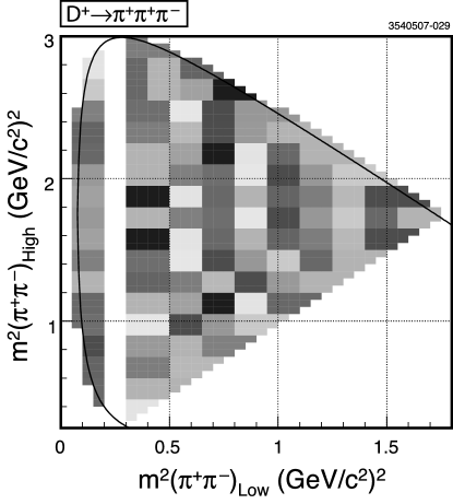
Figure 5:
The Dalitz plot for candidates.
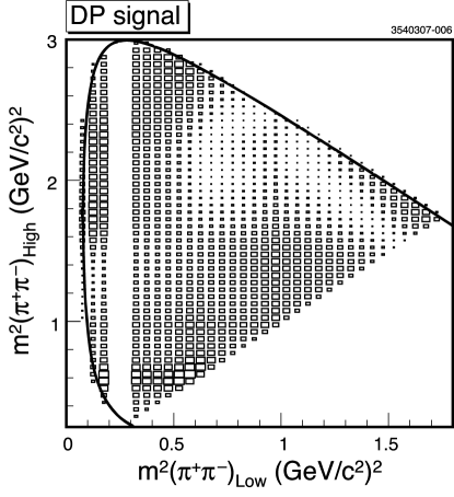
Figure 6:
The adaptive binning scheme.
III Event selection
Selection of events from the decay
is done with two signal variables:
(1)
(2)
where is a beam energy, and
and are the energy and momentum of
the reconstructed meson candidate, respectively.
The beam crossing angle of 4 mrad
is used to calculate the meson candidate energy and momentum
in the center of mass system.
We require
,
, where resolutions
MeV and
MeV/ represent the widths of
the signal peak in the 2D-distribution shown in
Fig. 2, and the projections,
Fig. 2 and
Fig. 4.
To determine the efficiency we use a GEANT-based Monte Carlo
simulation
where one of the charged meson decays in a signal mode
uniformly in phase space, while the other decays to
all known modes with relevant branching fractions.
Simulated events are
required to pass the same selection requirements as data.
The shape of the background contribution in
the Dalitz analysis is estimated
using events from the two hatched side-band boxes
shown in Fig. 2.
The sideband boxes are shifted in
to select the background events whose
invariant mass range is consistent with the signal box.
This selection gives 6991 events in the signal box.
From a fit to the distribution, shown in
Fig. 2, we find
215918 of these to be background.
The contribution to the sample of events in the signal box
is easily seen as a sharp peak in the invariant mass spectrum
shown in
Fig. 4.
The contribution is well described by a Gaussian shape
with resolution MeV/ both in data and
the simulation.
The number of events in the peak is 223977 from a fit
to a Gaussian signal plus linear background.
Excluding fraction and the background
leaves 2600 signal events of the decay.
From these yields we calculate branching fractions,
and
(statistical errors are shown only),
which are consistent with recently published CLEO-c results
Blusk and
HadronicBF .
This cross-check demonstrates the quality of our simulation
and validity of assumptions about the background level.
The presence of two mesons impose a Bose-symmetry
of the final state.
The Bose-symmetry when interchanging the two same sign charged pions
is explicitly accounted for in our amplitude parameterization.
We analyze events on the Dalitz plot by choosing
and
as the
independent (,) variables.
The third variable is dependent on and
through the energy-momentum balance equation.
This choice folds all
the data into the top half of the kinematically allowed region,
as is shown in Fig. 6.
The contribution from
is clearly seen as the narrow vertical band with
.
In our Dalitz plot analysis we do not consider events in the band
(GeV/)2,
which is approximately ten times our mass
resolution. This leaves 4086 (signal and background) events
for our Dalitz plot analysis.
IV Dalitz Plot Analysis
IV.1 Formalism
This Dalitz plot analysis exploits the
techniques and formalism described in Ref. Tim
that have been applied in many other CLEO analyses.
We use an unbinned maximum likelihood fit that minimizes
the sum over events:
(3)
where is the probability density function (p.d.f.), depends on
the event sample to be fit,
(4)
The shapes
for the efficiency, , and background, , are
explicitly symmetric, third order polynomial functions.
To account for efficiency loss in the corners of the Dalitz plot,
due to low momentum tracks that are not reconstructed,
we use three multiplicative threshold functions that drop
the efficiency to zero when one of the Dalitz variables , , or
is at their maximum values.
The background shape parameterization also
includes the non-coherent addition of three resonances
, , and .
The signal p.d.f. is proportional to the
efficiency-corrected matrix element squared, ,
whose fraction is .
We estimate from the fit to the mass spectrum
after removing events of the contribution.
The background term has a relative fraction.
The signal and the background fractions are normalized separately,
,
, which provides the overall p.d.f. normalization,
.
The matrix element is a sum of partial amplitudes,
(5)
where is a mass and spin-dependent function,
is an angular distribution Tim , and
is the Blatt-Weisskopf angular momentum barrier-penetration factor Blatt-Weisskopf .
In our standard fit the complex factor
is represented by two real numbers, an amplitude
and a phase . These are included in the list of fit parameters
and can be left to float freely or fixed.
For well established resonances, such as
,
,
,
,
, etc.,
is modeled with the Breit-Wigner function
(6)
where is the invariant mass,
and are the resonance mass and
mass dependent width Tim , respectively.
The parameterization of the ,
whose mass, , is close to the production threshold,
uses the Flatté Flatte formula
(7)
where and are the coupling constants of
the resonance to the
and final states, and
is a phase space factor, calculated for the decay
products momentum, , in the resonance rest frame.
We model a low mass S wave, or , in a number of ways.
To compare our results with E791 we try a simple spin-0 Breit-Wigner.
We also tested a
complex pole amplitude proposed in Ref. Oller_2005 :
(8)
where
GeV is a pole position in the complex plane
estimated from the results of several experiments.
We also consider two
comprehensive parameterizations of the low mass S wave.
One of them,
suggested by J. Schechter, is discussed in Section IV.3,
and its formalism is presented in Appendix VII.1.
Another one, suggested by N.N. Achasov,
is discussed in Section IV.4,
and its formalism is presented in Appendix VII.2.
IV.2 Fits with Isobar Model
We begin our Dalitz plot analysis
by attempting to reproduce the fit results E791 E791_Dp-pipipi .
Our amplitude normalization and sign conventions are different from E791.
We therefore compare the phases and fit fractions only.
In Fit#1 the contributions from
,
,
,
,
, and non-resonant intermediate states are included.
Fit#1 gives a probability of .
We checked that the inclusion of a contribution, Fit #2,
agrees better with the data giving a fit probability of .
We obtain good agreement comparing our results with
Fit#1 and Fit#2 discussed in Ref. E791_Dp-pipipi .
Then, we systematically study possible contributions from all known
resonances listed in Ref. PDG_2006 :
,
,
,
,
,
, and
.
We do not consider due to its negligible branching fraction
to .
We assume that high mass resonances
and
, having non-uniform angular distributions
at the edge of the kinematically allowed region, are well
enough represented by
, which is a dominated resonance.
The asymptotic “tails” of other known higher mass resonances,
,
,
are effectively accounted for in our fits
by the contribution.
We also include a unitary amplitude parametrization of the -wave
with isospin I=2 from Ref. Achasov_PRD67_2003 .
For the we use the Flatté formula, Eq. 7,
with parameters taken from the recent BES II measurement BES_2005 .
For the we switch to a complex pole amplitude, Eq. 8,
rather than the spin-0 Breit-Wigner used by E791.
Starting from the contributions clearly seen in our fit,
which is equivalent to Fit#2 of E791 E791_Dp-pipipi ,
we add or remove additional resonances one by one in order to improve the consistency
between the model and data.
We use Pearson’s statistic criterion PDG_2006 for adaptive bins
to calculate the probability of consistency between the p.d.f.
and the data on the Dalitz plot.
The bins are shown in Fig. 6.
We also consider the variation of the log likelihood to judge improvement.
We keep a contribution for the next
iteration if its amplitude is significant at more than three standard deviations and
the phase uncertainty is less than .
Table 2 shows the list of
Table 2: Results of the isobar model analysis of the Dalitz plot.
For each contribution the relative amplitude, phase, and fit fraction
is given. The errors are statistical and systematic, respectively.
Mode
Amplitude (a.u.)
Phase (∘)
Fit fraction (%)
1(fixed)
0(fixed)
20.02.30.9
1.40.20.2
12105
4.10.90.3
2.10.20.1
–12363
18.22.60.7
1.30.40.2
–211514
2.61.80.6
1.10.30.2
–441316
3.41.00.8
pole
3.70.30.2
–342
41.81.42.5
surviving contributions with their fitted amplitudes and phases, and calculated fit fractions.
The sum of all fit fractions is 90.1%, and
the fit probability is 28% for 90 degrees of freedom.
The best p.d.f. and the two projections of the Dalitz
plot and selected fit components are shown in
Figs. 7,
9, and 9.
Figure 7:
The signal p.d.f. for the isobar model fit described in the text.
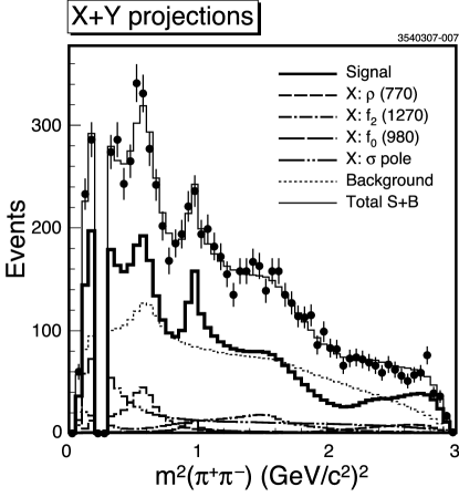
Figure 8:
Projection of the Dalitz plot onto the axis
(two combinations per candidate) for CLEO-c data (points)
and isobar model fit (histograms) showing the various components.
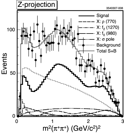
Figure 9:
Projection of the Dalitz plot onto the axis
for CLEO-c data (points)
and isobar model fit (histograms) showing the various components.
For contributions that are not significant we set
upper limits at the 95% confidence level, as shown in
Table 3. The “N.R.” represents a non-resonant contribution
which is assumed to populate the Dalitz plot uniformly with a constant phase.
Table 3: Upper limit on the fit fraction, at the 95% confidence level,
for contributions that we do not find significant in the
isobar model Dalitz plot analysis.
Mode
Upper limit on fit fraction (%)
2.4
N.R.
3.5
I=2 S wave
3.7
1.6
2
The systematic uncertainties, shown in Table 2,
are estimated from numerous fit variations.
We study the stability of the nominal fit results
by adding or removing degrees of freedom,
varying the list of contributions to the Dalitz plot,
changing the event selection, and varying the
efficiency and background parameterizations.
The systematic uncertainty of each fit parameter
is estimated as the quadratic sum of the mean and root mean square
values of the distribution of the changes in the parameter from
its value in the nominal fit.
For example for the poorly established resonances
, , and pole,
we allow their parameters to float and the variations
of the other fit parameters contribute to the systematic
errors. The nominal and fitted values of these
parameters are presented in Table 4.
The fit results when the parameters are allowed to float
do not vary from the nominal values by more than two standard deviations.
Table 4: Parameters for the poorly established resonances used in the nominal isobar model fit
and their fitted values when they are allowed float.
The isobar model drawbacks are most apparent in the
S wave sector where wide resonances overlap
and unitarity is not fulfilled.
The model of Joseph Schechter and co-workers in
Refs Schechter_2001 , Schechter_2005
is based on the meson part of the chiral invariant linear sigma model
sigma_model Lagrangian.
Poles are handled using K-matrix regularization which respects unitarity by definition.
Details of the parameterization are discussed in Appendix VII.1,
and here we only summarize the meaning of the fit parameters.
In our isobar model Dalitz plot fit the S wave
is represented by a complex pole for the ,
the Flatté for the and two Breit-Wigner for the and .
Schechter’s S wave amplitude, Eq. 22
(Appendix VII.1),
parameterizes simultaneously the mixed with the
in strong and weak interactions.
The Schechter model
describes the mixed and contributions to the Dalitz plot
with seven parameters:
the bare masses and ;
the strong mixing angle between the and ;
the total S wave amplitude and phase ;
and the relative weak amplitude and phase of the
with respect to the amplitude.
A combination of these parameters in the model
gives the total scattering phase, ,
and an overall S wave amplitude, , for the and contributions.
Operationally we replace the isobar and
contributions by the function of Eq. 22
times .
The Breit-Wigner’s parameterization is still used
for the and .
Table 5:
S wave amplitude parameters in the fit of the Schechter model described
in the text to the Dalitz plot.
Mode
#S1
#S2
#S3
(MeV/)
847
75836
74555
(MeV/)
1300
1385101
1221128
(∘)
48.6
455
389
4.10.2
3.90.4
4.50.6
(∘)
543
544
556
3.80.2
4.21.5
2.11.5
(∘)
233
225
215
(S wave)
45.91.9
46.44.8
4312
(%)
92.1
90.6
88.3
Pearson
116.3/96
100.4/93
99.6/87
Probability (%)
7.8
28.2
16.8
414
398
397.3
we fix all amplitudes and phases to their values from our isobar model fit,
fix the S wave model parameters as in Eq. 19,
float the S wave amplitude and phase ,
and float the relative amplitude and phase
in Eq. 22.
This fit gives a probability of which indicates
the Schechter model for the S wave is an acceptable description of the data.
In a second fit, #S2 in Table 5,
we start from the parameters obtained in #S1
and allow the bare masses , ,
and the strong mixing phase
in Eq. 22 to float.
This fit gives a probability of and
MeV/, which is
standard deviations lower than the values obtained in Ref. Schechter_2001 ,
as also shown in our Eq. 19.
The mass and the phase are statistically
consistent with the results in Ref. Schechter_2001 .
Fits #S1 and #S2 are used for an initial assessment of
the Schechter S wave parameters relative to the isobar model fit.
In a final fit, #S3 in Table 5,
we float the Schechter S wave model parameters and
all the parameters of the other contributions.
The results of fit #S3 are shown in
Figs. 11 and 11
in projections of the Dalitz plot.
Figure 13 shows the
isolated S wave contribution to the Dalitz plot, and
Fig. 13 shows the scattering phase, ,
defined in Eq. 20
in Appendix VII.1.
The total signal contribution is very similar to that shown in
Fig. 7.
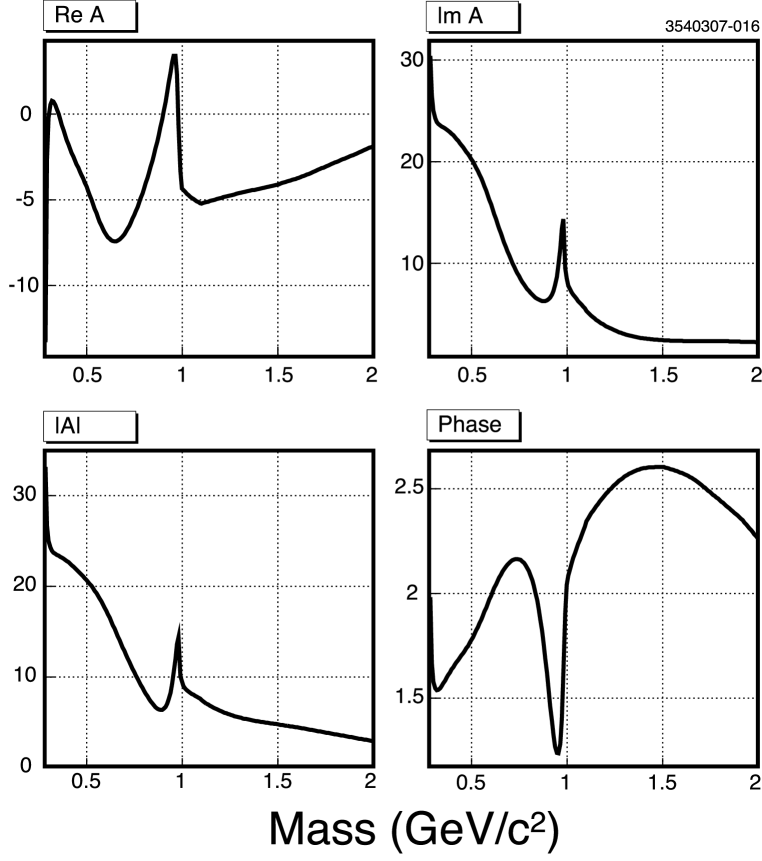
Figure 14
shows the complex amplitude from Eq. 22
as the real and imaginary parts, the magnitude and complex phase.
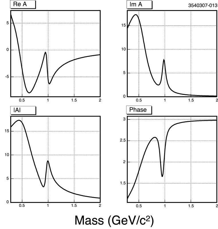
Figure 10:
Projection of the Dalitz plot onto the axis
(two combinations per candidate) for CLEO-c data (points)
and Schechter model fit #S3 (histograms) showing the various components.
Figure 11:
Projection of the Dalitz plot onto the axis
for CLEO-c data (points)
and Schechter model fit #S3 (histograms) showing the various components.
Figure 12: The isolated S wave contribution of
Schechter model fit #S3 on the Dalitz plot.
Figure 13: The
scattering phase , Eq. 20,
calculated for parameters
from Schechter model fit #S3 to the
Dalitz plot.
Figure 14:
Complex S wave amplitude from Schechter model fit #S3
to the Dalitz plot.
The real and imaginary parts, the magnitude and phase are shown
as a function of mass.
Employing the Schechter model changes the fit parameters
for the non S wave contribution by less than
the systematic uncertainties in the isobar model fit.
We also note that the amplitude and fractions of and
tend to be larger in the Schechter model fit.
This model gives an acceptable fit probability 17%
when it is used to describe the and fractions in our data.
The S wave fit fraction, (4312)%, is consistent with a sum of fit fractions from
, (41.81.42.5)%, and , (4.10.90.3)%
in the isobar model.
We find the Schechter S wave model parameters,
listed in Table 5,
are consistent with the values in Ref. Schechter_2001 .
Our data are consistent with both the isobar and Schechter models.
IV.4 Achasov Model
In Refs. Achasov_YF32_1980 –Achasov_PRD73_2006 and references therein,
a S wave interaction is studied for , ,
, and processes
in a manner motivated by field theory.
The S wave production and the final state interaction
(FSI) mechanism in meson three-body decays
have not yet been considered in the framework of this model.
In Ref. Achasov_D3pi the S wave amplitude in
decay is discussed.
The developed formalism is described in Appendix VII.2,
and here we only summarize the meaning of the fit parameters.
The Achasov model treats the S wave contribution to
via the sum of a number of amplitudes.
There is a contribution
from the non-resonant, point-like production amplitude;
direct resonance production via the
,
;
and the rescattering terms from several intermediate states,
,
, and
, to the final state.
Our parameterization has an amplitude, , and phase, ,
for the direct resonance production term,
accounting for the and components controlled by the coupling constants
and .
The contributions from rescattering have
amplitudes and phases parametrized by and
plus a parameter from loop diagram contributions, .
We explicitly fit for the “mode” = , , and
rescattering contributions.
The contribution from non-resonant is also
accoonted for the relevant point-like production amplitude parameter.
We start with the parameters,
shown in Table 2, where
the pole and are replaced by the S wave amplitude from
Eq. 75.
We fix all resonance parameters from our isobar model fit and
float different sets of S wave parameters to assess their range.
In four fits we float the amplitude,
, phase, , and the offset parameter, , (or
coupling constants and
in case of direct or meson production)
for sub-modes
,
,
, or “”, respectively.
For each of the single sub-modes we get a fit inconsistent with data.
In five fits we float , ,
(or and ) parameters
for each combination of two sub-modes.
All fits without the sub-mode
show probability of consistency with the data 10%,
while models with the sub-mode
are poorly consistent with the data.
In three fits we include three or more sub-modes.
These have a consistency with the data of 10%,
but give poor statistical significance for the amplitude parameters.
Fit #A1 allows full freedom for all the S wave sub-modes and
gives a probability of consistency with the data of 19%,
with 2–3 standard deviation significance for the amplitude parameters.
Its results are shown in Table 6.
We begin again with parameters of Fit #A1
and float or set to zero amplitude the parameters of
the , , and contributions
from our isobar fit.
In Fit #A2 we float all the S wave parameters and all
resonance parameters for the , , and contributions.
Variations of the nominal fit parameters, shown in
Table 2,
are within the range of the isobar model uncertainties.
Fit #A3 is like Fit #A2, but the
contributions from and scalar resonances are set to zero.
The fit quality change from Fit #A2 to Fit #A3 is small.
The S wave of the Achasov model has enough freedom
to substitute for the contribution of the and resonances.
The results of these two fits are shown in Table 6.
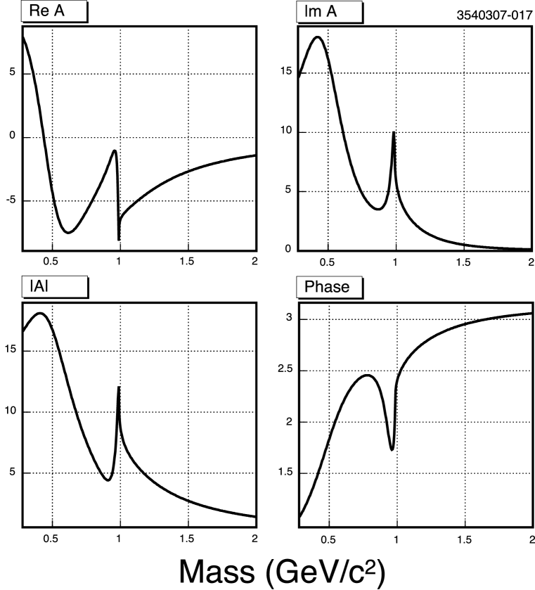
The results of Fit #A2 are shown in
Figs. 16–17
giving the Dalitz plot projections onto
the and axes, and
the representation of the S wave complex amplitude.
Our data are consistent with the isobar, Schechter, and Achasov models.
Table 6: Fit results for the Achasov model as described in the text.
Sub-amplitude,
#A1
#A2
#A3
parameters
1–fixed
1–fixed
1–fixed
–332
–667
–9213
2411
398
2112
2711
26724
13244
0.250.08
0.310.04
0.250.07
10412
709
939
1.50.3
2.20.2
2.90.3
0.560.39
1.350.15
1.800.40
11024
1077
8112
0.020.21
0.900.09
0.370.10
0.130.07
0.110.03
0.060.05
4131
14923
041
Fit fractions (%)
112.3
140.4
117.1
, 2
32.19.8
37.53.6
34.25.3
6.15.0
16.63.2
9.93.0
Fit goodness
100.7/89
96.9/83
106.8/87
Probability (%)
18.7
14.1
7.3
398.6
394.7
405.1
Figure 15:
Projection of the Dalitz plot onto the axis
(two combinations per candidate) for CLEO-c data (points)
and Achasov model fit #A2 (histograms) showing the various components.
Figure 16:
Projection of the Dalitz plot onto the axis
for CLEO-c data (points)
and Achasov model fit #A2 (histograms) showing the various components.
Figure 17:
Complex S wave amplitude from Achasov model fit #A2
to the Dalitz plot.
The real and imaginary parts, the magnitude and phase are shown
as a function of mass.
IV.5 Discussion of Models
We have tested three models of the low mass S wave in ,
and we find little variation of the parameters describing non S wave contributions.
The fit gives similar S wave contributions for all three models.
We show this by plotting the relevant complex functions describing the S wave.
Figure 18 shows the Flatté and the complex-pole
parameterizations for and , respectively,
for our isobar model fit to the data.
Figure 14 shows the results of the Schechter model fit, and
Fig. 17 shows the results of the Achasov model fit.
In Figs. 20, 20 we compare
the S wave amplitude and phase in the
accessible mass region from threshold to 1.7 GeV/ for these three models.
The solid curve corresponds to the Schechter model fit to our Dalitz plot,
the dashed curve is for Achasov model fit, and the
of the amplitude and phase parameters
range of the S wave contribution in the isobar model is indicated by the two dotted curves.
The S wave shapes are quite similar up to the interplay with other resonances,
and with the data set we have in hand
we are not sensitive to the details of the S wave parameterization.
Figure 18:
Complex S wave amplitude (complex pole for and Flatté for )
from isobar model fit
to the Dalitz plot.
The real and imaginary parts, the magnitude and phase are shown
as a function of mass.
Figure 19:
The S wave absolute amplitude for different models.
Figure 20:
The S wave phase for different models.
V Summary
Using a sample of 0.78 million
events collected in the CLEO-c experiment,
we performed a Dalitz plot analysis of the decay.
Our nominal results, obtained within the framework of the isobar model and
shown in Table 2,
reinforce the previous conclusion E791_Dp-pipipi , FOCUS_Dp-pipipi
that a sizable component is required,
in addition to other intermediate states
,
,
,
, and
, in order to describe the decay.
The systematic uncertainties are estimated by varying the fit parameters from
their nominal values.
We also show in Table 4
a set of optimal parameters for the , , and resonances
based on our isobar model fit to the Dalitz plot.
Limits on contributions from
,
non-resonant,
I=2 S wave,
, and
, shown in Table 3, are set at 95% confidence level.
We tested other models of the low mass S wave
contributions and in each case obtain optimal parameters.
In Table 5
we summarize results for the model suggested by J. Schechter and co-workers
Schechter_2005 , Schechter_2001 .
All fits for this model show consistent values for the parameters.
We also apply the S wave model suggested by N.N. Achasov et al.Achasov_D3pi .
This model has more freedom in sub-modes than we are confidently able to define with our data.
Possible solutions are presented in Table 6.
Further progress with this model can be achieved if several meson decay modes
with higher statistics are analyzed simultaneously.
Table 7: A comparison of the observed fit fractions () in % in the three
models of . For the “Isobar” column, the
“Low S wave ” entry is the sum of the two entries above.
Mode
Isobar
Schechter #S3
Achasov #A2
Low S wave
I=2 S wave
90.1
88.3
140.4
For all S wave models we find that their fit fraction exceeds 50%, and
confirm results of previous experiments of a significant contribution from
a low mass S wave in the decay.
Table 7 compares the fit fractions from the fits to the
three models described above.
The S wave fit fraction in Achasov model is three standard deviation
larger than in the Isobar and Schechter model.
The sum of all fit fractions is also larger in Achasov model, that indicates
on difference in interference terms.
The fit fractions for sub-modes are consistent between these three models.
Figures 20 and 20
compare the amplitude and phase, respectively, for the S wave
contribution we have found in the three considered models.
With our given data sample all three S wave parameterizations adequately describe
the Dalitz plot.
VI Acknowledgments
We thank Joseph Schechter, Amir Fariborz, and Nikolay Achasov
for stimulating discussions and significant help in application of
the low mass S wave models.
We gratefully acknowledge the effort of the CESR staff
in providing us with excellent luminosity and running conditions.
D. Cronin-Hennessy and A. Ryd thank the A.P. Sloan Foundation.
This work was supported by the National Science Foundation,
the U.S. Department of Energy, and
the Natural Sciences and Engineering Research Council of Canada.
VII Appendix: Alternative models of the S wave
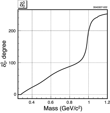
VII.1 Formalism of the S wave suggested by J. Schechter
A tree level scattering
amplitude for two resonances and
strongly-mixed with phase is given in
Eq. 3.2 of Ref. Schechter_2001 :
(9)
where
(10)
(11)
is the invariant mass squared,
and =0.131 GeV are the pion mass and the decay constant,
and are the bare masses of two scalar resonances,
and is a strong mixing angle.
We use the original notation of Ref. Schechter_2001 ,
the tilde is used for all parameters relating to
the second scalar resonance, ,
which in our case is associated with .
Equation 9 can be re-written as
(12)
where
(13)
(14)
(15)
According to the Dyson equation for the scattering,
Eq. 3.3 from Ref. Schechter_2001 gives an expression for a
total scattering amplitude through the tree amplitude:
(16)
The scattering amplitude is a complex number,
, then
the tree amplitude can be associated with the
tangent of the scattering phase,
(17)
and we get an expression for :
(18)
Expression
defines a scattering phase in the range
.
This phase has two discontinuities at
and
for parameters taken from
Ref. Schechter_2001 ,
(19)
In order to remove discontinuities we add a phase-shift above each bare mass:
(20)
where is a step function,
that makes the phase smooth, as shown in Fig. 13.
In this model the
production amplitude is obtained from the total scattering amplitude,
Eq. 16, by replacing the first tree level
scattering diagram amplitude,
, by the resonance propagator
with the coupling constant
and keeping the proper re-scattering amplitude, represented by the “bubble sum”
factor :
(21)
Extending Eq. 21
(Eq. 15 from Ref. Schechter_2005 )
for the case of two resonances and
we get the total production amplitude with relative weak interaction mixing factor
(22)
Note, that Eq. 22 does not contain singular terms because
both poles are contracted into the factor from ,
Eq. 15 and 18.
For the first iteration we set
(23)
It should be noted, that in the frame of this model,
is a scalar resonance which has a bare mass as a parameter.
The bare mass does not coincide with a peak position as in case of Breit-Wigner,
that is clearly seen in Eq. 19 for the mass of .
This simple model does not take in to account that the scalar resonances may have
other decay modes, coupled channels. For example, it is well known that
has a decay mode with a mass dependent rate as large as 20%.
Presumably, this amplitude, obtained from the chiral Lagrangian,
works well in the region close to the production threshold.
In the case of SU(3) symmetry it accounts for the two low mass resonances and .
Other higher mass resonances such as the and are not taken into account.
These issues restrict the precision and limit the application
of this model.
VII.2 Formalism of the S wave suggested by N.N. Achasov
VII.2.1 total amplitude
In this section we summarize a suggested formalism Achasov_D3pi for a parameterization
of the scalar amplitude in the decay, and
present the details of our implementation in the Dalitz plot fitter with some relevant
cross-checks.
For the decay Ref.Achasov_D3pi suggests
the use of a S wave amplitude that is a superposition
(24)
of a point-like, , direct resonance, ,
and non-resonant production terms, , , , followed by the re-scattering
in to the final state.
Here we list the definitions of all the sub-amplitudes in Eq. 24.
The point-like amplitude is associated with a constant :
(25)
After the point-like production one would expect
and scattering,
which we parametrize as a mass dependent amplitude
(26)
Functions , , and are described below.
An exotic I=2 S wave scattering is discussed in
Ref. Achasov_PRD67_2003
(27)
It is assumed that the and mesons can be produced directly
in the and decays
(we use the “” notation), with an amplitude of
(28)
The point-like amplitude is associated with another constant
(29)
Subsequent rescattering may also contribute to the final state via
the amplitude
(30)
In the above equations we assume that .
The point-like production amplitudes for and
are represented by the constants and ,
(31)
(32)
Then, two terms account for the relevant rescattering amplitudes
and
,
(33)
(34)
where we assume that offset parameters are equal, .
In above equations we use the function , which represents a contribution
from the loop diagram
(35)
where
(36)
(37)
Below all definitions, required for parametrization of the amplitude in our case,
are re-written from the recent Ref. Achasov_PRD73_2006 .
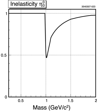
VII.2.2
Equation 23 from Ref. Achasov_PRD73_2006 gives the S wave amplitude of
scattering with I=0 is
The is an inelasticity for the wave with total spin and
isospin . In the mass range of (1.54 GeV)
the inelasticity parameter
should be represented by the smooth real function of .
An appropriate fit to data has been considered in Ref. Zou_Bugg_2004 ,
see their Fig. 2, and we use the approximation
(55)
In our case
we neglect the small wave scattering amplitude
.
VII.2.6 Mixing matrix
The mixing operator is a matrix of inverse propagators,
with rank equal to the number of mixed resonances.
In case of mixing of two resonances and this matrix has the form,
following Eq. 5 of Ref. Achasov_PRD73_2006 ,
(56)
In general, the diagonal elements of this matrix are the
inverse propagators
(57)
while the non-diagonal elements are polarization operators
describing mixing.
An expression for the inverse propagator of the scalar resonance is given in
Eq. 6 from Ref. Achasov_PRD73_2006 ,
(58)
where
takes in to account the finite width correction.
After Eq. 5 in Ref. Achasov_PRD73_2006 the non-diagonal terms of the
polarization operator are given by equation
(59)
where the constants take into account effectively the contribution
of , 4 and other intermediate states and incorporates the subtraction constants for the
transitions.
Here we use the notation from different publications, Achasov_PRD55_1997 –Achasov_PRD73_2006 ,
The constants are related to the width, Eq. 11 from Ref. Achasov_PRD73_2006 ,
(64)
VII.2.7 Model parameters
In the mixing operator Eq. 56 we account for
seven intermediate states:
,
,
,
,
,
, and
.
We follow the conventions of Ref. Achasov_PRD73_2006
for coupling constants, motivated by the four-quark model.
For the and similarly for the we use
(65)
For the coupling constants to we use
(66)
For the coupling constants to we use
(67)
Further
we use the values of the parameters shown in Table 8,
which are taken from Fit 1 of Ref. Achasov_PRD73_2006 .
Table 8: Achasov model parameters from Fit 1 of Ref. Achasov_PRD73_2006
used in our calculations.
Figure 21:
The background phase in scattering, ,
from Eq. 44.
Figure 22:
The phase of the resonance scattering,
, from Eq. 42.
Figure 23:
The total scattering phase,
, from Eq. 39.
Figure 24:
The inelasticity,
, from Eq. 41 for GeV/.
Figure 25:
The background phase in scattering,
, from Eq. 52 (solid curve),
and its approximation by the phase space factor (dashed curve).
Figure 26:
The total background phase in scattering,
,
from Eq. 49.
Figure 27:
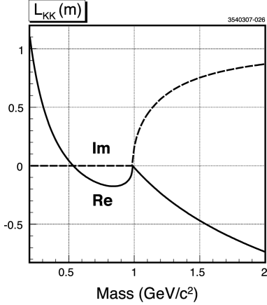
The loop integral, , from Eq. 35.
The real (solid curve) and imaginary (dashed curve) parts of the complex function are shown.
Figure 28:
The loop integral, , from Eq. 35.
The real (solid curve) and imaginary (dashed curve) parts of the complex function are shown.
VII.2.8 Check for , , , , etc.
In order to check that the code for this parameterization works
properly we reproduce plots from Ref. Achasov_PRD73_2006 .
:
We define the as the phase of the
complex function in Eq. 42.
However, this phase has discontinuities
in the vicinity of each resonance mass, but not exactly at the resonance mass value.
In further calculations we require that the phase is continuous, as shown in
Fig. 24,
by adding a phase shift of above each discontinuity point.
This plot is consistent with Fig. 3 in Ref. Achasov_PRD73_2006 .
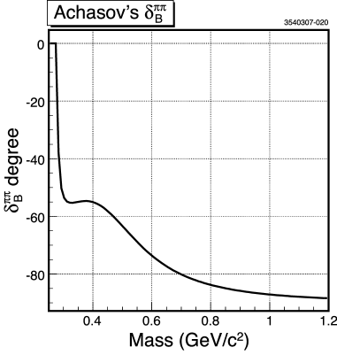
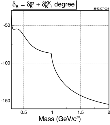
:
The background phase is derived from
Eq. 44, as shown in Fig. 24.
This plot is consistent with Fig. 2 in Ref. Achasov_PRD73_2006 .
:
The total phase represented by Eq. 39
is shown in Fig. 24. This plot is consistent with
Fig. 4 in Ref. Achasov_PRD73_2006 .
:
The derived from Eq. 41 is displayed in
Fig. 24 which shows that at
confirming unitarity in scattering,
consistent with Fig. 6 from Ref. Achasov_PRD73_2006 .
We also tested all complex functions and their components from
Eq. 24. In particular,
Fig. 26 shows from Eq. 52;
Fig. 26 shows from Eq. 49;
Figs. 28, 28 show the loop integrals
and , respectively,
from Eq. 35.
VII.2.9 S wave implementation in the code of the Dalitz plot fitter
As usually in a Dalitz plot analysis each amplitude fraction is taken with its own complex coefficient
represented by two real numbers, an amplitude and phase .
The loop integral in Eq. 35 has an additional offset constant
. Unitarity requires that is real.
All these constants, as well as unknown coupling constants
and from
Eq. 45,
are the fit parameters, which can be free to float or fixed.
The actual parameterization for
or
is given by the amplitude
(68)
(69)
(70)
(71)
(72)
(73)
The I=2 scattering amplitude for
is given by
(74)
It is worth noting that three terms in
Eqs. 68,
69 and
74
have a common complex coefficient ,
appearing from the point-like term, and two of them have a common offset parameter
from the loop integral.
The total contribution of Achasov’s S wave in the Dalitz plot amplitude is
(75)
The “” sub-mode in Eq. 73
has a redundant freedom for amplitude factors due to the products
and .
In our fits we fix , or to turn it off,
and use coupling constants and .
For a first approximation we try to eliminate the number of free parameters in the function.
We assume and
from isospin symmetry.
We note that the parameterization for
in Eq. 72
is nearly the same as that for
in Eq. 71.
The small difference appears due to the different masses of the and mesons.
Keeping in mind this small difference between amplitudes we do not consider separate contributions
from in this analysis. This means that the amplitude factor
includes both contributions from
and
.
The amplitude for in Eq. 70
has a different isospin factor at compared to
the amplitude for in Eq. 69 and
different masses for and .
In our fits we assume the equity .
The constant also accounts for the point-like term in
Eq. 68, and is involved in I=2 term,
Eq. 74, that makes it different from
the .
For this reason we consider the sub-mode separately
from .
References
(1) P.L. Frabetti et al. (E687 Collaboration),
Phys. Lett. B 407, 79 (1997).
(2) J.C. Anjos et al. (E691 Collaboration),
Phys. Rev. Lett. 62, 125 (1989).
(3) E.M. Aitala et al. (E791 Collaboration),
Phys. Rev. Lett. 86, 770 (2001).
(4) J.M. Link et al. (FOCUS Collaboration),
Phys. Lett. B 585, 200 (2004).
(5) R.H. Dalitz, Philos. Mag. 44, 1068 (1953).
(6) J.A. Oller, Phys. Rev. D 71, 054030 (2005).
(7) D.V. Bugg, Phys. Lett. B 632, 471 (2006).
(8) S.M. Flatté, CERN/EP/PHYS 76-8, 15 April 1976; Phys. Lett. B.63, 224 (1976).
(9) J. Schechter, Int.J.Mod.Phys. A20, 6149 (2005).