NBODY meets stellar population — The HYDE-PARC Project

Abstract

Aims. $N$-body simulations give us a rough idea of how the shape of a simulated object appears in three-dimensional space. From an observational point of view this may give us a misleading picture as a stellar system consists of both bright and faint stars. The faint stars may be the most common stars in the system but the morphological information obtained by observations of an object may be dominated by the color properties of the bright stars. Due to dynamical effects, such as energy equipartition, different masses of stars may populate different regions in the object. Since stars are evolving in mass the stellar evolution may also influence the dynamics of the system. Hence, if one is interested in simulating what the morphology will look like through a telescope, one needs to simulate in addition evolving stars and weight them by their luminosity.

Methods. Therefore we need to combine simulations of the dynamical evolution and a stellar population synthesis at the same time. For the dynamical evolution part we use a parallel version of a direct $N$-body code, NBODY6++. This code also includes stellar evolution. We link the parameters from this stellar evolution routine to the BaSeL 2.0 stellar library. This allows us to obtain a spectrum and colors for each star in the simulated cluster. We call this the HYDE-PARC project, which means Hybrid Code for Dynamical Evolution and Population Analysis of StellaR Clusters.

Results. We tested our method by simulating globular clusters with up to 50000 stars and investigating the integrated colors. For isolated clusters we found results assimilable to standard stellar population synthesis codes such as the PEGASE code. For clusters in a tidal field we found that the integrated colors become relatively bluer due to energy equipartition effects. In the time shortly before dissolution of the cluster the stellar M/L ratio becomes lower compared to isolated clusters. We compared the results of our simulations to integrated spectra of galactic globular clusters. For the cluster NGC 1851 we found good agreement between simulation and observation. For extragalactic clusters in M81 and M31 we looked at medium band spectral energy distributions and found for some clusters also a good agreement.

1 Introduction

Globular clusters are among the oldest objects in a galaxy and also among the oldest objects in the universe. Hence, the investigation of these objects is crucial for the understanding of the historical evolution of their host galaxies. Furthermore, these clusters provide an interesting environment for investigating dense stellar systems. In these star clusters collisions between stars happen more often than in other places in the Galaxy, where typical collision timecales of stars would exceed the lifetime of the Galaxy or even the age of the universe (Davies 2002, Portegies Zwart 2000). In these systems the effects of stellar dynamics and stellar evolution are important and interact with each other. For example, stellar evolution in close binaries takes place differently than in single stars due to their mutual interaction, which may cause mass transfer. On the other hand, stellar evolution changes the stellar mass, and therefore influences the dynamical evolution of the system.

Local globular clusters in our galaxy can be resolved in single stars and therefore investigated in a detailed manner, for example in terms of color-magnitude diagram (CMD) morphologies. For more distant extragalactic globular clusters both the resolution and the faintness are an issue, even when using contemporary instruments such as the Hubble Space Telescope (HST) and 8m class telescopes. The amount of information available for those objects is comparable to that obtained for clusters in local group galaxies in the early 1990s (Forbes 2002). Since one has to deal with unresolved objects, integrated properties such as spectra and colors of the whole stellar population are available. Therefore one needs to find a way how to derive as much information as possible by just looking at integrated spectra or integrated colors. Due to the combination of dynamical evolution and stellar evolution mentioned above this task is more complicated than, for example, investigating the integrated spectra of galaxies.

Examples of more recent observations are the spectroscopy of globular clusters in M81 by Schroder et al. (2002), and the medium-band spectral energy distributions (SEDs) now available for globular clusters in M81 (Ma et al. 2006a) and in M31 (Ma et al. 2006b). Narbutis et al. (2006) presented UBVRI broad band photometry of 51 compact star clusters in M31. Also, spectra of the NGC 1399 globular clusters are published by Kissler-Patig et al. (1998) and those of the NGC 4365 clusters are published by Larsen et al. (2001). Kundu et al. (2005) did deep HST observations of the cluster system of NGC 4365 and NGC 1399, and found that NGC 4365 has a number of globular clusters with bluer optical colors than expected for their red optical-to-near-infrared colors. In terms of color, a bimodality of the color distribution of globular cluster systems is well-known. The first statistical test for bimodality of elliptical galaxy globular cluster colors was already presented by Zepf & Ashman (1993).

In order to deal with such problems, one may consider two different approaches: (i) follow the evolution of the stars; or, (ii) follow the dynamical evolution of the stellar system.

The first approach is that of stellar population synthesis models. These models follow the evolution of a population of stars. Stars are assumed to be born with a certain initial mass function and a certain star formation rate, which may vary in time. Evolutionary models of stars then follow the evolution tracks of stars in the CMD according to their mass. Chemical enrichment is also taken into account, because the yields of supernova explosions will enrich the interstellar medium with metals. Therefore, the next generation of stars will have a higher metallicity. The stellar parameters of these stars are transformed into spectra and colors by using stellar libraries. The summation of the spectra of all stars lead to integrated properties of the whole stellar population such as integrated spectra and integrated colors. There are various codes which follow (in principle) this approach, among them there are those of Fioc & Rocca-Volmerange (1997), Bruzual & Charlot (2003), Anders & Fritze-v. Alvensleben (2003) and Maraston (2005). Recently, Fagiolini et al. (2006) published a Monte Carlo simulation of star clusters and addressed the issue of populating stars randomly in stellar clusters with limited star numbers.

The second type of models are $N$-body simulations where a sample of $N$ particles interact with each other by gravity. Direct $N$-body simulations follow the dynamical evolution of such a sample of particles with high precision. For each particle, which may be regarded as a “star”, the trajectory in space will be followed by calculating the force due to the mutual interaction with other stars. In dense stellar systems such as globular clusters the dynamical behavior is therefore strongly influenced by the gravitational interaction with all other stars. As mentioned before, the dynamical evolution may be influenced by the evolution of the stars themselves. During its evolution a star may change in mass, and therefore its dynamical behavior depends on this mass change. Stellar evolution may take place differently in double stars. Direct $N$-body codes can also follow the dynamical evolution of double stars, which are important for the dynamical behavior of the whole system.

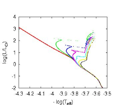
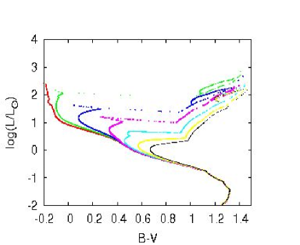
Figure 1: Color-magnitude diagram for a simulation with 50000 particles. The left plot shows the effective temperature versus luminosity. The parameters $T_{\rm eff}$ and $\log g$ are drawn from the stellar parameters mass, radius and luminosity, delivered by the hrplot routine of the NBODY6++ code. These stellar parameters are transformed into spectra and colors by using the stellar library BaSeL.2. The right diagram shows the B-V color instead of the temperature. The color coding is the following: red: 0 Gyr, green: 0.5 Gyr, blue: 1 Gyr, purple: 2 Gyr, light blue: 5 Gyr, yellow: 10 Gyr, black: 15 Gyr.

Hence, these two types of models follow different aspects of the stellar system. The first one describe the evolution of integrated properties of the whole system. Therefore, these models are useful for unresolved objects such as distant globular clusters in other galaxies. The second describes the dynamical evolution of the stellar system. Therefore, these models are useful for investigations of the dynamical properties of a system, such as the velocity dispersion.

The ideal approach would be a combination of both a $N$-body simulation and a stellar population synthesis model. In the case of globular clusters, a good approach would be to assume that each simulation particle represents one star. Since the stars have different masses, which may change due to stellar evolution, the stars themselves may influence the dynamical properties of the system. Effects such as mass segregation due to energy equipartition may occur. This means that the high-mass stars sink to the center, whereas the low-mass stars are more in the outer regions. Conversely, the dynamical evolution may change the stellar populations or even the stellar evolution. For example, a globular cluster evolving in a tidal field of a host galaxy may remove in particular low-mass stars from the cluster, which would cause a depletion of low-mass stars leading to a bluer color of the cluster.

One should mention that there are other approaches. For example, Ivanova et al. (2005) presented a Monte Carlo approach combining a population synthesis code and a simple treatment of dynamical interactions in the dense cluster core using a tool for three- and four-body interactions. This approach focusses more on the evolution of binary fractions in globular clusters. This is in principle also possible with the approach mentioned above, but expensive in terms of computation time. However, the first approach has the advantage that the dynamical behavior of the whole cluster can be modeled more directly.

In this paper we follow the idea of combining $N$-body simulations with stellar populations synthesis. The method is described in section 2. Results of test simulations are shown in section 3. In section 4 we compare these results to observational data of integrated colors and spectra of globular clusters. Conclusions are drawn in section 5, and section 6 gives an outlook of our future work.

2 Method

As discussed above, we want to combine direct $N$-body simulations with stellar population synthesis modeling in order to model the dynamical evolution and color evolution of globular clusters at the same time. Following this approach, we are developing the HYDE-PARC (Hybrid Code for Dynamical Evolution and Population Analysis of StellaR Clusters).

For this purpose the NBODY6++ code (Spurzem 1999) is used, which is a parallel version of the Aarseth NBODY4 code (Aarseth 1999). Simple recipes to follow the changes of stellar masses, radii, and luminosities due to stellar evolution have been implemented into NBODY4 and NBODY6++ (Hurley et al. 2001), in the sense that each simulation particle represents one star. These prescriptions cover all evolutionary phases and solar to globular cluster metallicities. We used the stellar parameters obtained by this stellar evolution routine and coupled them to the stellar library BaSeL 2.0 (Lejeune et al. 1997).

The $N$-body code uses a high-precision (4th order) direct $N$-body integrator, which allows us to follow stellar dynamical two-body relaxation as well as all kinds of close encounters between singles and binaries with high efficieny and precision and without any artificial change of the interaction potential (no softening). Such codes, containing a Hermite scheme, hierarchically blocked individual variable time steps, Ahmad-Cohen neighbour scheme, and regularisations of two-body and higher encounters are being developed and supported by Aarseth (1985, 1999a, 1999b, for the general $N$-body code) and Mikkola (1997) and Mikkola & Aarseth (1990, 1993, 1996, 1998, for the regularisation methods). We use the special version NBODY6++ (Spurzem 1999), which is the only one available to use on massively parallel computers (supercomputers as well as PC Beowulf clusters, recently also including GRAPE accelerator cards).

The globular cluster is modeled as a spherical stellar system with a Plummer sphere. In future, rotating models will also be investigated, such as used in Einsel & Spurzem (1999). The mass of each simulation particle (representing one “star”) is selected using a certain initial mass function (IMF). In the work presented here a Kroupa et al. (1993) IMF is chosen. When the simulation is started, the stars begin to evolve and follow their evolution as given by the stellar evolution recipes (Hurley et al. 2000). In the language of stellar population synthesis modeling this corresponds to single stellar evolution – in future also binary evolution will be incorporated. While $N$-body simulations are scale-free, stellar evolution requires us to fix the time scale.

The NBODY6++ code provides the stellar parameters mass $M$, radius $r$ and bolometric luminosity $L$ of each star. By using

$$T_{\rm eff}^{4}=\frac{L}{4\pi r^{2}\sigma}$$ (1)

and

$$g=\frac{GM}{r^{2}}$$ (2)

these parameters are transformed into $T_{\rm eff}$ and $\log g$.

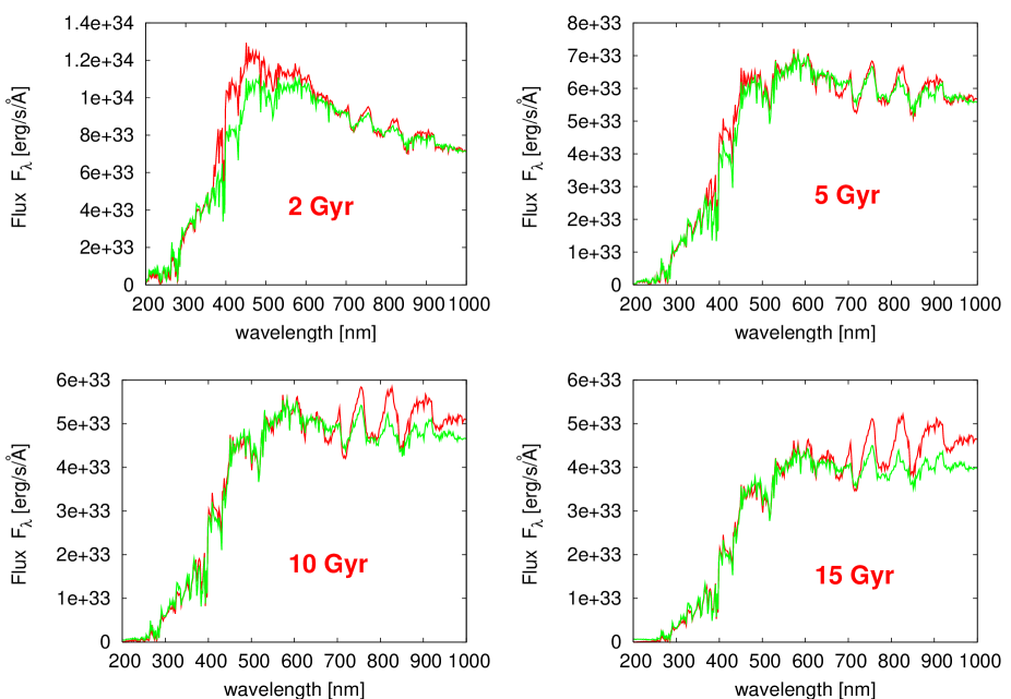
Figure 2: Integrated spectrum of a isolated cluster at 4 different ages. The red spectra show the result from the simulation of the NBODY6++ code. The green spectra show the result from the PEGASE code.

Since the NBODY6++ code deals with a single stellar population, the metallicity value, $Z$, is the same for all stars. Together with the effective temperature $T_{\rm eff}$ and the $\log g$ value delivered by the formula (1) and (2) the simulation delivers a parameter triple for each star.

For a stellar library we use the BaSeL 2.0 library of Lejeune et al (1997). It is organized as a grid defined in the $(Z,T_{\rm eff},\log g)$ space. Some interpolation is necessary in order to transform the library into a regular grid in terms of these parameters: in particular for cool stars with temperatures below 3500 K we need to interpolate the surface gravity at some values in order to match the parameter values to the grid given by the higher temperature stars. In addition, at some metallicities there are some “holes” in the parameter grid, and therefore we need to interpolate in order to fill the mesh point gaps.

Hence, the library grid fits to the parameter triple described above. Therefore, this parameter triple can be interpolated to the parameter grid of the library. This leads to a spectrum that can be attached to each star.

For example, Figure 1 shows the CMD for a simulation of 50000 particles. The effective temperature plotted in the left diagram is converted into the B-V color in the right diagram by using the BaSeL 2.0 library.

The spectra of all stars can be added in order to get the integrated spectrum of the entire stellar population. A convolution of the integrated spectrum with filter curves delivers integrated colors. For test purposes so far only the Johnson filter set is used.

3 Results of test simulations

For test purposes we investigate several simulations. For the mass distribution we use a Kroupa IMF (Kroupa et al. 1993) with an upper mass of 8.16 M_⊙ and a lower mass of 0.16 M_⊙. We use only single stars without primordial binaries. Also no binary evolution is taken into account. We use a Plummer model, both for the isolated cluster and also for the cluster in the tidal field. In the latter case, for the external force a standard tidal field is used, that corresponds to a cluster orbiting at a distance of 8.5 kpc around the galactic center in a circular orbit. For most cases we use initially 50000 particles, except in cases where other particle numbers are mentioned.

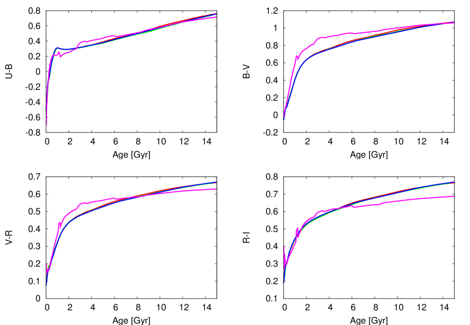
Figure 3: Integrated colors of a isolated cluster as a function of age. Color coded are different particle numbers: red: 10000 particles, green: 20000 particles, blue: 50000 particles. As a comparison, the purple lines show the time evolution of colors calculated with the PEGASE code.

3.1 Comparison with the PEGASE code

First we will concentrate on the integrated spectra and colors of an isolated cluster. Since the BaSeL 2.0 library is also used in the PEGASE code (Fioc & Rocca-Volmerange 1997) it is also interesting to compare the results of the NBODY6++ simulations to the results from the PEGASE code. Figure 2 shows the integrated spectra at the ages 2 Gyr, 5 Gyr, 10 Gyr and 15 Gyr. At low ages there is a difference between the NBODY6++ result and the PEGASE result in the regime around 400 nm - 600 nm. This difference vanishes towards higher ages. In the wavelength regime above 700 nm there is a mismatch that increases toward higher ages.

The time evolution of integrated colors shown in Figure 3 reflects consequently the mismatches mentioned above. The difference in B-V color reaches its maximum at around 3 Gyr. Towards higher ages the NBODY6++ result and the PEGASE result are converging. Corresponding to the behavior at higher wavelengths the R-I colors of both codes match best at lower ages. Towards higher ages there is an increasing mismatch. As seen in Figure 2, in the lower wavelength regime the results of both codes are in good agreement. This is reflected in the time evolution of the U-B color in Figure 3, which shows good agreement in the results of both codes at all ages.

The difference between the PEGASE results and the NBODY6++ results is most likely due to the different treatment of stellar evolution. One reason is the issue of the thermally-pulsing asymptotic giant branch (TP-AGB) stars. These stars are rare, but bright, and therefore already a few of these stars in the whole cluster are enough to influence the integrated spectrum, in particular at longer wavelengths. In the current version presented here the TP-AGB stars are not included. This issue will be addressed in the future work.

As expected for an isolated cluster, the time behavior of all colors is practically independent of the particle number.

The results discussed do far are obtained at solar metallicity. The metallicity dependence of integrated colors is shown in the following figures. Figure 4 shows the metallicity dependence of different optical colors at different ages. A comparison of the results of both codes still shows good agreement at most metallicities. For solar metallicities it reflects the result seen in Figure 3: the agreement is better for higher ages. Interestingly, there is a certain mismatch for lower metallicities. This low metallicity mismatch is even higher for V-R colors, and also present for R-I colors.

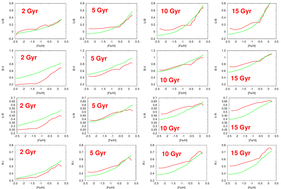
Figure 4: Integrated colors of a isolated cluster as a function of metallicity. Each row shows one color according to the colors: U-V, B-V, V-R, R-I. Each column shows one age of the cluster. The color coding means the following: red: NBODY, green: PEGASE result.

3.2 Influence of the tidal field

We also investigated the influence of the tidal field of a host galaxy on the integrated color evolution of the globular cluster. Owing to the tidal field particles are removed from the cluster when leaving the tidal radius. Therefore the cluster is disrupted and the particle number is monotonically decreasing. The result of the integrated B-V color is shown in Figures 5 and 6. Figure 5 shows the results for different particle numbers. As a result, the color evolution of a tidally disrupted cluster follows more or less the evolution of a isolated cluster for most of its lifetime. Only shortly before the cluster will be dissolved, it becomes first slightly bluer and then it becomes dramatically redder.

Figure 6 shows the result for different $\bar{R}$ values. The $\bar{R}$ value gives the virial cluster radius in pc. Therefore it controls the concentration of the globular cluster by a given distance of the cluster center to the gravity center. Note, that a variation of $\bar{R}$ is physically equivalent to a variation of the galactocentric distance. However, this is only true in the dynamical sense in a scale-free language. But in the simulation here the stellar evolution sets a second timescale, and therefore the physical timescale is fixed and the system can no longer be considered as being scale-free. Since the $\bar{R}$ value influences the dynamical timescale, whereas the stellar evolution timescale is fixed, a certain physical time of the system mean different NBODY6++ time units in simulations with different $\bar{R}$ values.

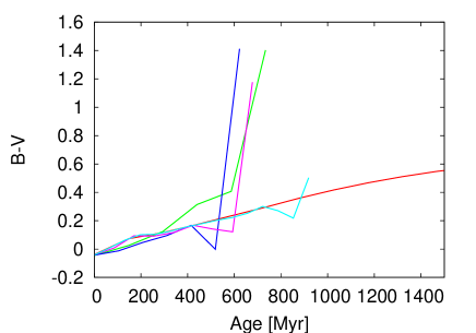
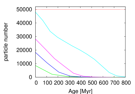
Figure 5: Color evolution of the globular cluster influenced by the tidal field of the host galaxy. This simulation is done for a virial cluster radius of $\bar{R}=30$ pc. Color coded are different initial particle numbers. Left plot: B-V color, right plot: time evolution of the particle number. Color coded are different initial particle numbers: green: 10000, blue: 20000, purple: 30000, light blue: 50000. As a comparison, the red line shows a isolated cluster.

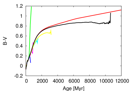
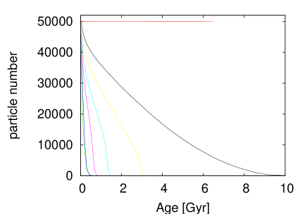
Figure 6: Color evolution of the globular cluster influenced by the tidal field of the host galaxy. Left plot: B-V color, right plot: time evolution of the particle number. Color coded are different virial cluster radii, given in the code as $\bar{R}$ values: green: $\bar{R}$ = 50, blue: $\bar{R}$ = 40, purple: $\bar{R}$ = 30, light blue: $\bar{R}$ = 25, yellow: $\bar{R}$ = 20, black: $\bar{R}$ = 15. As a comparison, the red line shows a isolated cluster.

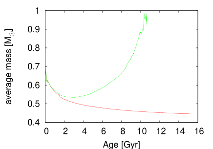
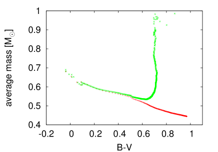
Figure 16: Evolution of the average mass per star. The red line shows the isolated cluster and the green line shows the a cluster influenced by a tidal field with $\bar{R}=15$. The left plot shows the time evolution, whereas the right plot shows the average mass evolution in terms of the B-V color.

For large $\bar{R}$ values corresponding to a low cluster concentration the evolution shows a similar behavior as seen in Figure 5. However, when the $\bar{R}$ value is low enough, the cluster lifetime increases drastically, and becomes significantly bluer compared to the isolated cluster. This is due to the effect of mass segregation. In order to investigate this effect, Figure 16 shows the average particle number for both simulations, for an isolated cluster and for the simulation with the lowest $\bar{R}$ value. The isolated cluster shows a decreasing average mass due to stellar evolution effects. The cluster in the tidal field shows a strong upturn in average mass. This is due to the effect of mass segregation. Resulting from this the low-mass stars escape from the cluster, and therefore the average mass increases up to 1 solar mass. Hence, the origin for the bluer color is a loss of low-mass particles in the stellar population.

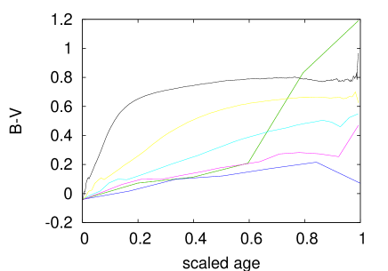
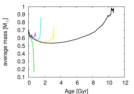
Figure 7: Left plot: Same as Figure 6 (left). This time the age is scaled to the dissolution time. Therefore, for every simulation at age = 1 the cluster is dissolving. Color coded are different $\bar{R}$ values: green: $\bar{R}$ = 50, blue: $\bar{R}$ = 40, purple: $\bar{R}$ = 30, light blue: $\bar{R}$ = 25, yellow: $\bar{R}$ = 20, black: $\bar{R}$ = 15. Right plot: evolution of average mass per particle. The color coding is the same.

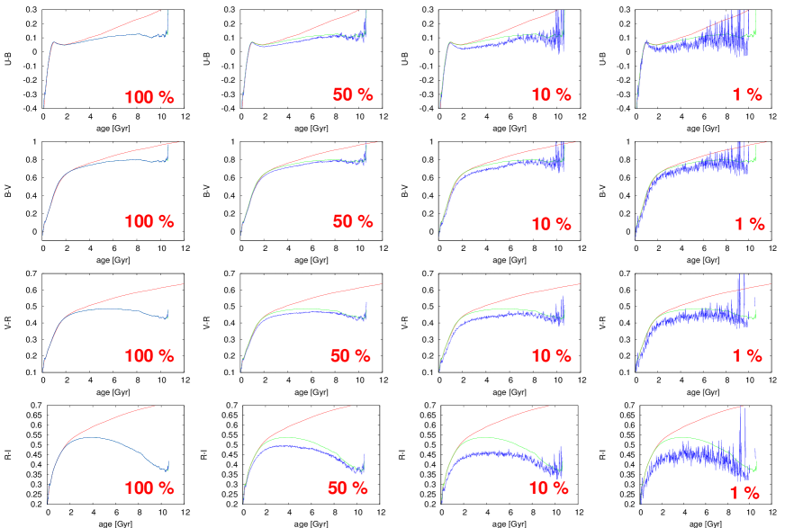
Figure 8: Colors of the globular cluster influenced by a tidal field at different Lagrange radii. The green curves include all particles of the whole cluster. The blue curves include all particles within a certain Lagrange radius. Each row shows one color according to the colors: U-V, B-V, V-R, R-I. The four columns correspond to four different Lagrange radii: 100%, 50 %, 10% and 1%. As a comparison, the red curve shows the color evolution of the isolated cluster.

At the time of dissolution the particle number naturally becomes very low. Due to statistical fluctuations the average particle mass may become very low or very high. This is shown in Figure 7 (right), where the average particle mass is shown for the same set of $\bar{R}$ values as shown in Figure 6 For example, at $\bar{R}=50$ there are only two particles in the last time before the simulation ended, and both are low mass stars, resulting in a low average particle mass. This causes a strong jump in B-V color, as shown in Figure 6. On the other hand, for $\bar{R}=25$ there are 9 particles at the final time. Among them, there are two particles with masses around 0.9 solar masses, resulting in a higher average mass at the last time step.

We investigated the dependence of the mass-to-light ratio on the B-V color. It is shown in Figure 15. The left plot shows a simulation of a globular cluster with 50000 particles. The result can be well described as a straight line fitted to the data. The right plot shows a simulation of a globular cluster with $\bar{R}$=15 influenced by a tidal field. From Figure 6 we know that this cluster also lives for several Gyrs and shows bluer colors compared to the isolated cluster. In Figure 15 this effect of bluer color corresponds to a sharp edge around B-V = 0.7. At this edge there is a strong deviation in M/L ratio, when comparing to the color-M/L correlation of the isolated cluster. The reason for this M/L ratio deviation is a strong increase in the average mass at that color. This is shown in Figure 16 (right), that exactly at this color the average mass increases due to the effect of the escape of low-mass stars in clusters in a tidal field. Since these low-mass stars have a higher M/L ratio, the cluster M/L ratio is decreasing, when the cluster loses low-mass stars.

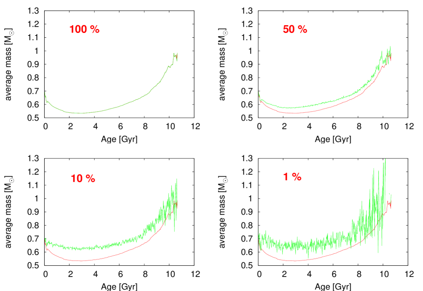
Figure 9: Time evolution of the average mass per star of the globular cluster influenced by a tidal field at different Lagrange radii. The red curves include all particles of the whole cluster. The green curves include all particles within a certain Lagrange radius. The four plots correspond to four different Lagrange radii: 100%, 50 %, 10% and 1%.

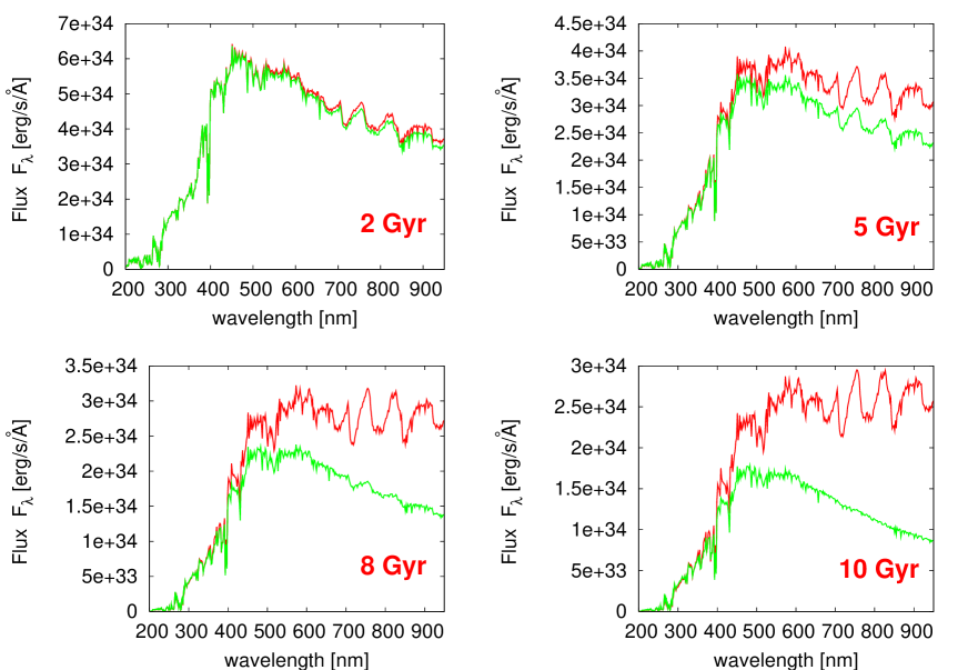
Figure 10: Integrated spectra of stellar clusters at different time steps. The red spectra show an isolated cluster, whereas the green spectra show a cluster in a tidal field.

It is interesting to notice that Figure 16 (right) shows that the color remains constant during the period when the M/L ratio is increasing. This reflects a balance between two different effects. Firstly, the cluster becomes redder due to the effect of stellar evolution and, secondly, the cluster becomes bluer due to the loss of red low-mass stars. Since the total luminosity is dominated by the main sequence turnoff, it is able to balance the loss of low-mass stars, which are larger in number, but also fainter. Altogether, it turns out that in this phase the integrated color of the cluster is close to constant. This effect is already seen in Figure 6. The black curve in this figure shows little evolution in B-V color at ages from 3 to 10 Gyr.

The results presented so far include all particles contained in the simulated cluster. In Figure 8 we show the dependence of color evolution on radial position from the cluster centre, by utilising the Lagrangian radii. The Lagrange radius gives us at each timestep the radius containing a certain fraction of the mass of the cluster. Four different Lagrange radii are shown containing 100 % of the cluster mass down to 1 % of the cluster mass. The plots show the same simulation as discussed in Figures 6 and 15, which is a cluster in a tidal field with $\bar{R}$ = 15. As shown in Figure 8, the difference is negligible for U-B colors and for B-V colors, whereas there is a strong radius dependence in the R-I colors. In Figure 9 we investigated the average stellar mass at different Lagrange radii. As a result, in the inner 10% there is a parallel shift in the sense that the average stellar mass is higher in the inner regions. Hence, the higher mass stars are more located in the inner regions, whereas the lower mass stars are more located in the outer regions. This effect reflects the decreasing R-I color in the inner 10%: In the longer wavelength regime we expect to see the red, low mass, stars and therefore the R-I color becomes bluer in the inner regions, where these stars become underrepresented compared to the higher mass stars.

So far we have only looked at the integrated colors. It is also interesting to look at the spectra. Figure 10 compares the integrated spectrum of an isolated stellar cluster with the spectrum of a cluster in a tidal field with $\bar{R}=15.$ As we have seen in Figure 2, the isolated cluster behaves like a simple stellar population modeled by usual stellar population methods. In comparison, the cluster in the tidal field loses more and more flux at longer wavelengths. This is what we already noticed in the color plots – the cluster becomes bluer compared to the isolated cluster. In addition, the spectral features at longer wavelengths become less pronounced at higher ages, compared to the isolated cluster.

Figure 11 shows the spectra at different Lagrange radii. Here we see again the effect of mass segregation, that alters the spectra in the inner part of the cluster in the sense that the fluxes at higher wavelengths are lowered in the inner part of the spectrum. This is due to the lack of red low-mass stars in the cluster center.

So far, all simulations are done with the same metallicity of [Fe/H] = 0 and with the same galactocentric distance, in the sense that the cluster is orbiting at the position of the Sun with respect to the Galactic center. Figure 12 shows simulations of clusters with different metallicities. The influence of the galactocentric distance is shown in Figure 13. It shows simulations of clusters circulating around the center at a distance of 4 kpc and at 8.5 kpc. At 5 Gyr the cluster with a radius of 4 kpc is dissolved, whereas the cluster at 8.5 kpc lives for about 10 Gyr until the cluster is dissolved. One can see from Fig. 12 and Fig. 13 that both effects have a dramatic effect on the spectra, in particular at higher ages.

We also investigate the radial distribution of integrated colors. Figure 14 shows these color distributions. Since we deal with relatively low particle numbers, which become even lower at higher ages, we decided to plot cumulative radial distributions. We show both the radial distribution in 3D space, and the projected radial distribution in the 2D plane as well. Whereas the 3D distribution has a more physical meaning, the projected 2D distribution brings our results closer to the observations, because clusters can only be observed as a 2D projection on the sky. As we can see in these plots, the 2D projected profiles are less steep than the 3D profiles. This is of course a projection effect.

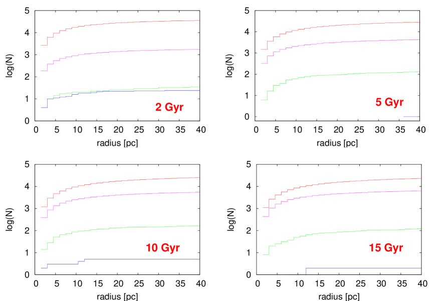
Figure 24: Radial distribution of stars. The different colors are different stellar types. Red: main sequence stars, green: red giants, blue: AGB stars, purple: white dwarfs.

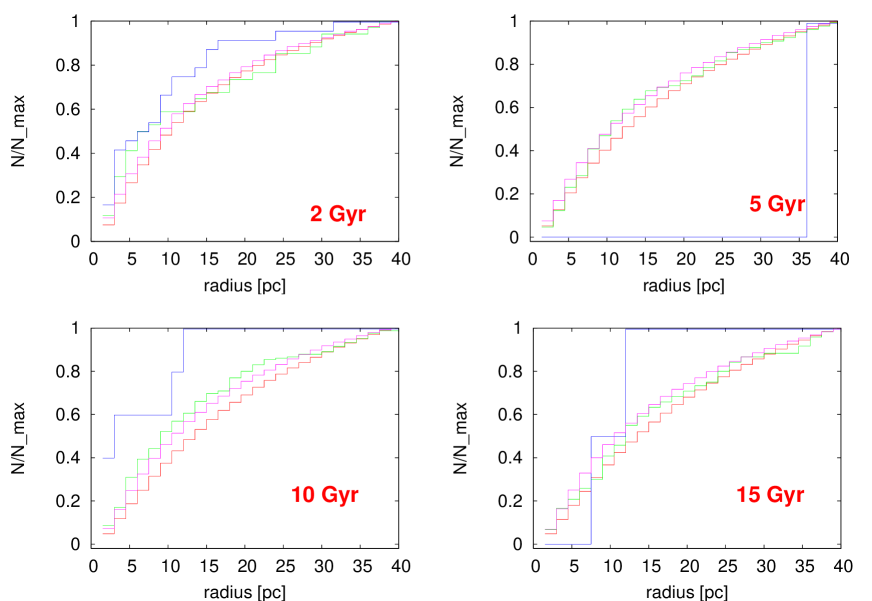
Figure 25: Radial distribution of stars, normalized to 1. The different colors are different stellar types. Red: main sequence stars, green: red giants, blue: AGB stars, purple: white dwarfs.

In Figure 24 we show cumulative plots of the radial distribution of different stellar types. Whereas the total number of main sequence stars is slightly decreasing, the number of red giants increases by a factor of 3 between 2 Gyr and 5 Gyr. The number of AGB stars is low, and the number of white dwarfs increases monotonically. Figure 25 shows the same cumulative plots but with the number counts are normalized to 1.

Table 1: Numbers of different stellar types in a simulation of a globular cluster in a tidal field with a initial particle number of 50000. At 4 different ages the total number of stars of a certain type is shown, and the number of stars, which are just escaping at that time. The different stellar types are: 1 = main sequence stars, 2 = red giants, 3 = AGB stars , 4 = white dwarfs, 5 = neutron stars, 6 = black holes.

Star	1 Gyr		2 Gyr		5 Gyr		8 Gyr
type	total	esc.	total	esc.	total	esc.	total	esc.
1	34240	248	26287	234	9485	108	1357	33
2	28	0	58	1	77	0	40	1
3	9	1	8	0	1	0	1	0
4	1687	17	2427	32	2218	46	670	15
5	0	0	0	0	0	0	0	0
6	0	0	0	0	0	0	0	0

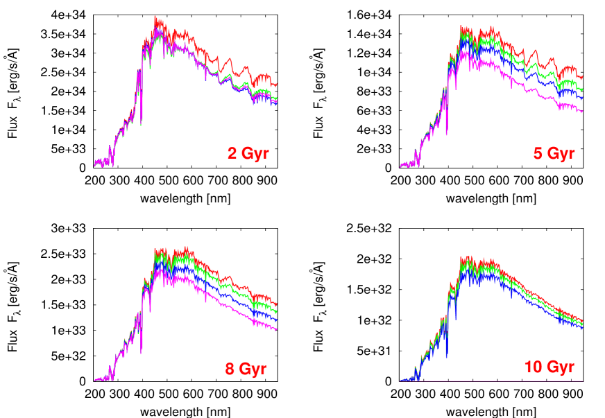
Figure 11: Spectra of the cluster in the tidal field, as shown in the green spectrum in Figure 10. Color coded are different Lagrange radii. Red: 100% enclosed mass, green: 50%, blue: 10%, purple: 1%.

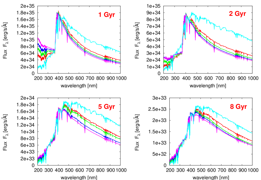
Figure 12: Integrated spectra of a clusters in a tidal field with different metallicities. The color coding is as following: red: [Fe/H] = -0.7, green: [Fe/H] = -1.0, blue: [Fe/H] = -1.2, purple: [Fe/H] = -1.5, light blue: [Fe/H] = 0.0.

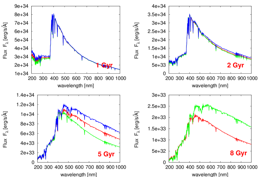
Figure 13: Integrated spectra of a clusters in a tidal field with diffferent galactocentric distances. The color coding is as following: red: R = 8.5 kpc, green: R = 4 kpc, blue: R=16 kpc. In order to arrange the cluster lifetime in a useful range, the $\bar{R}$ values are chosen in a certain way: $\bar{R}$ = 15 for R = 8.5 kpc, $\bar{R}$ = 10 for R = 4 kpc, and $\bar{R}$ = 20 for R = 16 kpc.

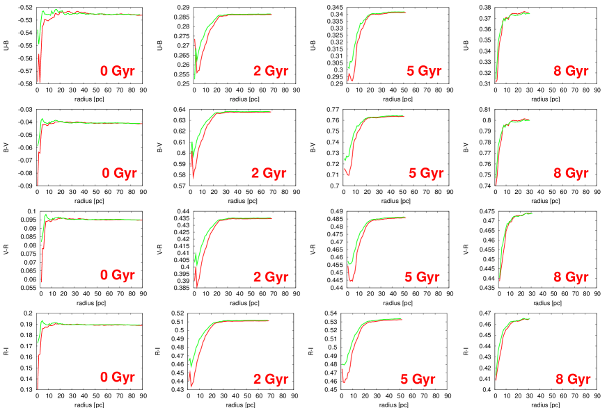
Figure 14: Cumulative color radial distribution of the cluster in the tidal field. Each row shows one color according to the colors: U-V, B-V, V-R, R-I. Each column shows one age of the cluster. The red curve shows the color distribution of all particles which are enclosed in concentric spheres of different radii. The green curve shows the color distribution which are enclosed in concentric circles in the XY-plane.

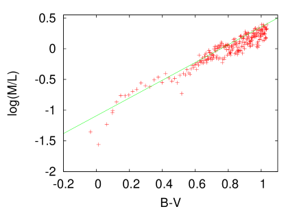
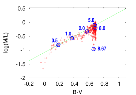
Figure 15: B-V colors versus mass to light ratio for a globular cluster with 50000 particles. Each dot represents the integrated B-V color and the total M-L value for a certain timestep. The left plot shows a isolated cluster. The right plot shows a cluster influenced by a tidal field with $\bar{R}$ = 15, wich corresponds to the black line in Figure 6. The green line in both plots is a least square fit to the points in the left plot. The blue numbers in the right plot label certain ages in Gyr.

4 Comparison to the observations

The results presented in the last section can be regarded as predictions which need to be compared with observational results. So far, we have restricted ourselves to integrated properties such as integrated colors and integrated M/L ratios. In order to compare these results to observations, we take the integrated colors of galactic globular clusters from the Harris catalogue (Harris et al. 1996). Integrated M/L ratios were taken from Illingworth (1976) and from Mandushev et al. (1991) by using their mass estimations from single-mass King models. The comparison to our predicted color-M/L relation is shown in Figure 17 In addition, we take the M/L ratios from Pryor & Meylan (1993), who use a family of multi-component King-Mitchie models to estimate their masses. The comparison of those M/L values with our simulations is shown in Figure 18. Whereas the single-mass estimations of the first two authors deliver M/L ratios, which are systematically at the lower end of our predicted M/L values, the Pryor & Meylan values match well the range of M/L ratios predicted by our simulations. In more detail, for the simulation of the isolated cluster a large fraction of objects still mismatches the simulated results, whereas for the cluster in the tidal field the whole sample of objects is in a M/L regime that matches the simulated values, when the low-M/L-tail is taken into account. In terms of colors almost a certain fraction of objects are redder than the color edge predicted in the simulations. However, the exact value of the color-edge depends on the parameters of the simulation. This effect is demonstrated in Figure 20, which shows simulations with different parameter combinations. The origin for the point cloud in Figure 18 is therefore a mixture of different parameters for the different galactic globular clusters.

One should be aware of the fact that the mass estimations of these authors rely on models which are different from the model considered here. If one were aiming at self consistence, a better test would be to compare directly the velocity dispersions used by these authors with those predicted by our models. Such direct comparison is shown in Figure 19. It shows the velocity dispersion and the core radius of galactic globular clusters. This can be compared to our simulated globular cluster, for which the corresponding parameters are shown as a purple curve, which represents the time evolution of the simulated cluster. From Figure 19 we conclude that the core radii of the simulated cluster are within the regime of those core radii occuring for galactic globular clusters, for the entire lifetime of the simulated cluster. In the beginning the velocity dispersion of the simulation is in a region where galactic globular clusters are present, but at the end of the simulation it becomes too low by a factor of 10. The reason is our low particle number, which leads to a relatively low cluster mass, in particular at higher ages, where the cluster has lost a large fraction of its initial mass.

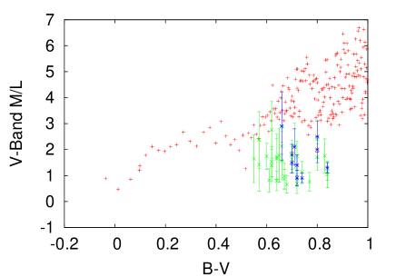
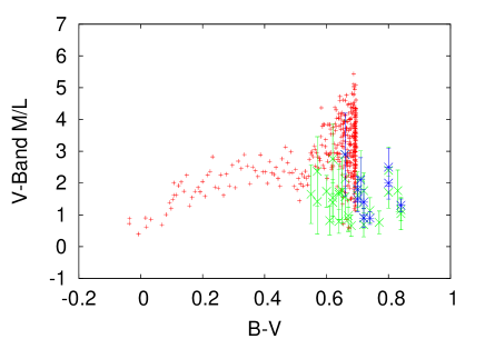
Figure 17: Comparison of the measured B-V color vs. M/L ratio correlation to our simulation results, as shown in Figure 15. The left plot shows the simulation of a isolated cluster, whereas the right plot shows the simulation of a cluster in a tidal field. The integrated colors of galactic globular clusters are from the Harris catalogue (Harris 1996). The M/L ratio estimations are from Illingworth (1976) (blue points) and from Mandushev et al. (1991) (green points). From both authors we use the M/L values estimated by using a single mass King model.

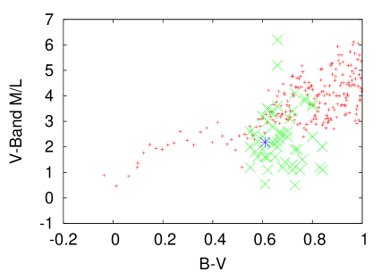
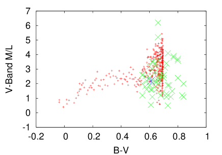
Figure 18: Same as Figure 23. This time we use the M/L ratio estimations from Pryor & Meylan (1993), who use multi-component King-Mitchie models for their mass estimation. The blue point is NGC 2298, for the mass we use the value given in De Marchi & Pulone (2006).

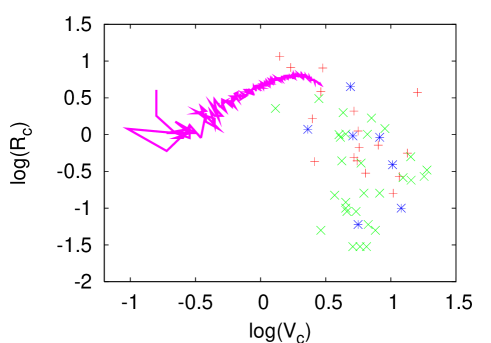
Figure 19: Velocity dispersion vs. core radius for galactic globular clusters, as listed in Pryor & Meylan (1993), who summarized these values. The authors who published these values are given as references in (Pryor & Meylan 1993). Color coded are different intervals of M/L ratios estimated by (Pryor & Meylan 1993): Red: 0.5 $\leq$ M/L $\leq$ 1.6, green: 1.8 $\leq$ M/L $\leq$ 3.5, blue: 3.6 $\leq$ M/L $\leq$ 6.2. As a comparison, our simulated cluster is shown as a purple line, which represents the time evolution of these parameter values.

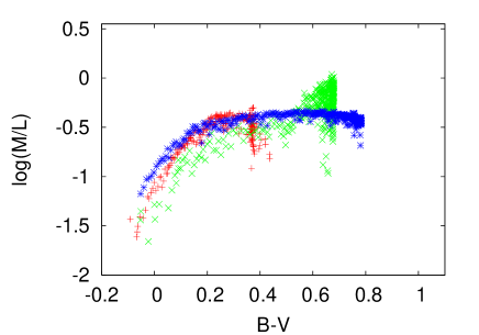
Figure 20: Mass-to-light ratio vs. B-V color for clusters in a tidal field. This time simulations with different parameters are shown. The left figure shows different metallicities: red: [Fe/H] = -0.7, green: [Fe/H] = -1.0, blue: [Fe/H] = -1.2, purple: [Fe/H] = -1.5. The right figure shows different galactocentric distances: red: 4 kpc, green: 8.5 kpc, blue: 16 kpc.

In order to compare our results in terms of spectra to the observations, we use the library of integrated spectra of galactic globular clusters published by Schiavon et al. (2005). This library contains 40 cluster spectra covering the range of 335 - 643 nm with 0.31 nm resolution. The sample of globular clusters contains objects with a wide range in parameters such as metallicity and galactocentric distance. We compared these spectra with our simulated spectra. Since all spectra are very different, most spectra do not match at all to our simulated one. By chance we found one object, whose spectrum matches quite well with our simulated one. It is NGC 1851, which has a metallicity of [Fe/H] = $-1.22$ and a galactocentric distance of 16.7 kpc, when looking to the Harris catalogue. Whereas the metallicity matches perfectly to our simulated one, the galactocentric distance is twice the value we simulated. This comparison is shown in Figure 21.

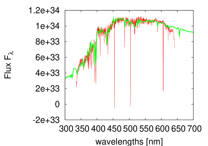
Figure 21: Comparison of the integrated spectrum of NGC 1851 measured by Schiavon et al. (2005) to our simulated spectrum of a cluster in a tidal field.

Table 2: Comparison of model parameters for M31 globular cluster SED’s observed by Ma et al. (2006 b).

Object	age [Gyr]		metallicity [Fe/H]
name	Ma et al.	this	Ma et al.	this
	(2006 b)	work	(2006 b)	work
M 009	2.92 $\pm$ 0.65	8	-0.63 $\pm$ 0.06	-1.0
M 013	7.65 $\pm$ 1.03	8	-1.10 $\pm$ 0.06	-1.0
M 024	9.34 $\pm$ 1.86	8	-1.46 $\pm$ 0.22	-1.0
M 035	4.36 $\pm$ 0.44	8	-1.70 $\pm$ 0.15	-1.0

We compare our results also to extragalactic globular clusters. Ma et al. published spectral energy distributions of 42 M81 globular clusters (Ma et al 2006 a) and of 15 M31 globular clusters and 30 cluster candidates (Ma et al 2006 b) in 13 intermediate band filters from 400 to 1000 nm. We compared them to our integrated spectra by eye.

Figure 23 shows the 4 best matching results in the M81 case. For these four objects the long-wavelength upturn above $\approx$ 600 nm is reproduced very well. The 4 best matching results in the M31 case are shown in Figure 24. If we neglect the first filter with a central wavelength of 421 nm, these four examples match the simulated spectrum even better than in the M81 case.

Ma et al. (2006 b) tried to estimate ages and metallicities of the M31 globular clusters by $\chi^{2}$ fitting of Bruzual-Charlot models to their 13 filter SEDs. Of course, a dircet comparison to our model does not make sense, because our method of creating stellar populations is entirely different from that of the Bruzual Charlot model in the case of globular clusters in a tidal field. Another issue is the well-known age-metallicity degeneracy.

However, it is interesting to see how their fit parameters relate to our model paramters. Whereas our simulation has in all four cases the same age and metallicity, the Ma et al. fits span a range between 2.9 Myr and 9.3 Myr in age, and a range between -0.6 and -1.7 in metallicity. We think that at least for the upturn at wavelengths above 600 nm our one model fits all four spectra well.

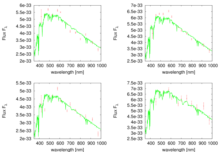
Figure 22: Comparison of the SED’s of M81 globular clusters measured by Ma et al. (2006 a) to our simulated spectrum of a cluster in a tidal field. For the object in the left plot in the lower panel an age of 5 Gyr is suitable, for the other objects the spectrum with an age of 8 Gyr fits good.

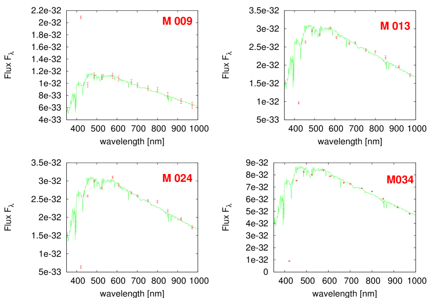
Figure 23: Comparison of the SED’s of M31 globular clusters measured by Ma et al. (2006 b) to our simulated spectrum of a cluster in a tidal field. For all four objects the spectrum at an age of 8 Gyr fits good.

5 Conclusion

The comparison of the NBODY6++ results and the PEGASE results of the integrated spectra shows an agreement which is at least promising. When comparing at solar metallicity, there is a good agreement at short wavelengths, reflecting a good agreement in the U-B color at all ages. The main difference occurs at low ages in the medium wavelength regime and at high ages in the longer wavelength regime. When looking to the metallicity dependence the situation becomes even more complex.

In both cases the BaSeL 2.0 library is used for transforming stellar parameters into spectra and colors. The difference at wavelengths above 700 nm, which occurs in the 15 Gyr plot, is probably due to the TP-AGB stars. There are no TP-AGB stars taken into account in this work.

For the cluster in the tidal field one would expect that the cluster becomes bluer. Energy equipartition is expected to sort the particles by mass in the sense that high-mass particles sink to the cluster center, whereas low-mass particles have a higher probability to escape from the cluster after leaving the tidal radius. Hence, one would expect that the escape of red low-mass stars leads to a relatively bluer integrated color. Indeed, there exists at least a parameter combination where the cluster becomes bluer, when the concentration is high enough and the lifetime is long enough compared to the stellar evolution lifetime.

The last two results raise the question of how the tidal field also influences the mass to light ratio. In Figure 15 the M/L ratio is compared for an isolated cluster and for a cluster influenced by a tidal field. The isolated cluster shows a very good correlation between color and M/L ratio. A similar correlation was also found by Bell and de Jong in the case of spiral galaxies (Bell & de Jong 2001).

For the cluster in the tidal field we chose the $\bar{R}$=15 case (black line in Figure 6). It shows significantly the expected bluer colors and lives for several Gyr. In this case there is a significant deviation in the M/L ratio at the red edge. Hence, the Bell & de Jong-like correlation is no longer true for clusters in a tidal field in the final disruption phase. Whereas a Bell & de Jong-like correlation can be used to determine the stellar mass of isolated clusters, one would introduce considerable deviations when using it for clusters influenced by a tidal field.

The comparison to the observed color-M/L ratio correlation shows a good agreement between observations and our simulations in terms of the V-band M/L ratios. The observed M/L ratios tend to confirm the lower values predicted by our model of a cluster in a tidal field rather than the model of a isolated cluster.

However, one should be aware that the observed M/L estimations depend also on a certain model. In one case this is a one-component King model, in the other case these are multi-component King-Mitchie models. The comparison of these model-dependent estimations to our simulations is of course not self-consistent. Therefore we also compared the observables themselves, namely the central velocity dispersion and the core radius, to our simulation, and we found values which are at least present among the sample of galactic globular clusters.

In terms of colors our observed color-edge on the red side is confirmed by the observations for a certain fraction of objects. However, there are still lots of objects above our predicted color-edge, and therefore we need more simulations with different parameters. For example, a lower $\bar{R}$ value would increase the cluster lifetime and therefore leads to a redder color edge.

The overall impression of Figure 18 is that our model of the cluster in a tidal field matches the observations of galactic globular clusters quite well. Since a cluster in a tidal field cannot be modeled with ordinary stellar population synthesis models, we have here a direct test for the validity of neglecting the effects of dynamical evolution of globular clusters. Another interesting feature is the cluster NGC 2298, which is the blue point in Figure 18. Recently, De Marchi & Pulone (2006) published an investigation of this object and claim that this cluster is on its way to disruption. In our comparison to the model this object lies exactly at the predicted color edge, and the M/L ratio also fits well to our predicted value. Therefore, this object fits nicely in our picture of a tidally disrupted cluster.

Integrated colors and spectra are tailored to objects which are too far away to be resolved into single stars. But also for galactic globular clusters integrated colors and spectra are available, and in spite of the existence of more detailed data we will use them in order to figure out what we can learn by just observing integrated SEDs.

Therefore, we compared the integrated spectra of our simulations to observed spectra of galactic globular clusters. In the case of the globular cluster NGC 1851 we find a good agreement of the integrated spectrum to our simulated spectrum. In terms of parameters, the cluster has a similar metallicity to our simulated cluster, and the galactocentric distance is twice the value in our simulation.

After demonstrating the power of integrated spectra in the case of galactic globular clusters we applied it to extragalactic objects, namely the globular cluster systems of M81 and M31, for which observed medium band SEDs are available in the literature.

For these SEDs we find a good agreement between our simulation and several M81 globular cluster SEDs. In the case of the M31 globular cluster SEDs the agreement is even better. We conclude from this, that our simulations lead to results, with are at least present among the globular cluster systems of these two galaxies.

6 Outlook

6.1 Detailed parameter study

So far, we have demonstated, that for simulations with certain parameters the results are able to to explain observations of some globular clusters. In future, more simulations will allow us to cover broader regions of the parameter space. $\chi^{2}$ fitting techniques will show in more detail possible parameter degeneracies and therefore the explanatory power of integrated spectra of distant globular clusters.

6.2 Mixed stellar populations

All simulations presented so far in this work are done with single stellar populations in the sense that all stars have the same age and the same metallicity. However, in future we are planning to deal also with mixed stellar populations. This means we want to allow for different stellar populations with different ages and different metallicities in the same simulation. As a first step towards a mixed stellar population we start with two different populations with different metallicities.

Our approach is realized in the code in such a way that every second star in a simulation has one metallicity $Z_{1}$ and the other stars have another metallicity $Z_{2}$. All these stars are distributed over a Plummer Sphere and are therefore ideally mixed. In future one may also think about a initial spatial distribution of different metallicities, for example a merger of two globular clusters with different metallicities.

Figure 26 shows our result of a simulation of a isolated cluster with two different metallicities. For large ages the B-V colors are exactly in between the colors of a single stellar population of one of these two metallicities. We conclude that these result is very promising and we will further go into the direction of mixed stellar polulations.

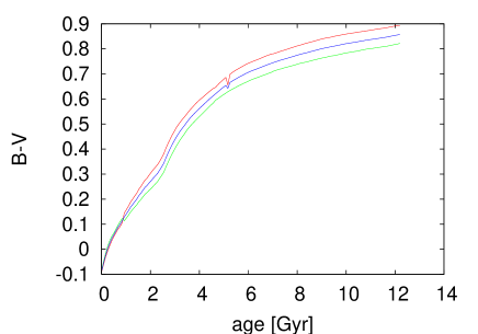
Figure 26: Mixed stellar populations with two different metallicities. The blue curve shows a simulation of a globular cluster containing two stellar populations with different metallicities: $Z_{1}=Z_{\odot}$ and $Z_{2}=\frac{1}{10}Z_{\odot}$. As a comparison, in the red and green curves only particles of the same metallicity are plotted. populations with the red curve being the upper metalllicity $Z_{1}$ and the green curve being the lower metallicity $Z_{2}$.

References

- (1) Aarseth, S.J., IAUS 113, 251-258 (1985)
- (2) Aarseth, S.J., PASP 111, 1333-1346 (1999)
- (3) Aarseth, S.J., CeMDA 73, 127-137 (1999)
- (4) Anders, P., Fritze-v. Alvensleben, U., A&A 401, 1063-1070 (2003)
- (5) Bell, E.F., de Jong, R.S., ApJ 550, 212-229 (2001)
- (6) Bruzual, G., Charlot, S., MNRAS 344, 1000-1028 (2003)
- (7) Davies, M., Phil. Trans. R. Soc. Lond. A, 360, 2773-2786 (2002)
- (8) Einsel, C., Spurzem, R., MNRAS 302, 81-95 (1995)
- (9) Fagiolini, M., Raimondo, G., Degl’Innocenti, S., astro-ph/0609162
- (10) Forbes, D.A., ASP Conf. Ser. (2002)
- (11) Fioc, M., Rocca-Volmerange, B., A&A 326, 950 (1997)
- (12) Harris, W.E., AJ 112, 1487 (1996)
- (13) Hurley, J.R., Tout, C.A., Aarseth, S.J., Pols, O.R., MNRAS 323, 630-650 (2001)
- (14) Illingworth, G. , ApJ 204, 73-93 (1976)
- (15) Ivanova, N., Belcyski, K., Fregeau, J.M., Rasio, F.A., MNRAS 358, 572-584 (2005)
- (16) Kissler-Patic, M., Brodie, J.P., Schroder, L.L., Forbes, D.A., Grillmair, C.J., Huchra, J.P., AJ 115, 105-120 (1998)
- (17) Kroupa, P., Tout, C.A., Gilmore, G., MNRAS 262, 545-587 (1993)
- (18) Kundu, A., Zepf, S.E., Hempel, M., Morton, D., Ashman, K.M., Maccarone, T.J., Kissler-Patig, M., Puzia, T.H., Vesperini, E., ApJ 634, L41-L44 (2005)
- (19) Larsen, S., Forbes, D., Brodie, J., Schroder, L., Grillmair, C., AJ 121, 2974 (2001)
- (20) Lejeune, T., Cuisinier, F., Buser, R., A&AS 130, 65-75 (1998)
- (21) Ma, J., Zhou, X., Burstein, D., Chen, J., Jiang, Z., Wu, Z., Wu, J., PASP 118, 98-106 (2006)
- (22) Ma, J., Zhou, X., Burstein, D., Yang, Y., Fan, Z., Chen, J., Jiang, Z., Wu, Z., Wu, J., Zhang, T., A&A 449 143-149 (2006)
- (23) Mandushev, G., Spassova, N., Staneva, A., A&A 252, 94-99 (1991)
- (24) Maraston, C., MNRAS 362, 799-825 (2005)
- (25) De Marchi, G., Pulone, L., astro-ph/0612026
- (26) Mikkola, S., Aarseth, S., CeMDA 47 (1989-1990) (1990)
- (27) Mikkola, S., Aarseth, S., CeMDA 57 (439-459) (1993)
- (28) Mikkola, S., Aarseth, S., CeMDA 64 (197-208) (1996)
- (29) Monelli, M., Corsi, C.E., Castellani, V., Ferraro, I., Iannicola, G., Prada Moroni, P.G., Bono, G., Buonanno, R., Calamida, A., Freyhammer, L.M., Pulone, L., Stetson, P.B., ApJL 621, L117-L120 (2005)
- (30) Narbutis, D., Vansevicius, V., Kodaira, K., Sableviciute, I., Stonkute, R., Bridzius, A., Baltic Astronomy 15, 461-469 (2006)
- (31) Portegies Zwart, S.F., ASP Conf. Ser. 211, 181-189 (2000)
- (32) Pryor, C., Meylan, G., ASP Conference Series, 50, 357-371 (1993)
- (33) Schiavon, R.P., Rose, J.A., Courteau, S., MacArthur, L.A., ApJS 160, 163-175 (2005)
- (34) Schroder, L.L., Brodie, J.P., Kissler-Patig, M., Huchra, J.P., Phillips, A.C., AJ 123, 2473 (2002)
- (35) Spurzem, R., JCoAM 109, 407-432 (1999)
- (36) Zepf, S.E., Ashman, K.M., MNRAS 264, 611 (1993)