Note on Chiral Symmetry Breaking from Intersecting Branes

Abstract

In this paper, we will consider the chiral symmetry breaking in the holographic model constructed from the intersecting brane configuration, and investigate the Nambu-Goldstone bosons associated with this symmetry breaking.

April 2007

1 Introduction

In [1], the author proposed that type IIB string theory on the space $AdS_{5}\times S^{5}$ is dual to $\mathcal{N}=4$ supersymmetric gauge theory on the boundary of this geometry, i.e the AdS/CFT correspondence. Using this method, one can study strongly coupled physics at zero and finite temperature [2, 3, 4, 5]. Since there exist no flavor degrees of freedom in the above constructions, in [6], flavor D-brane probes were introduced into the holographic D-brane constructions in order to get more realistic models. Along this line, there are many further developments [7, 8, 9, 10, 11, 12] of holographic models with flavor.

In the framework of these holographic D-brane constructions, many properties of strongly coupled gauge theory have been investigated. For example, in [8, 9, 10, 11, 12, 13, 15, 18, 19], chiral symmetry breaking has be studied in various dimensional gauge theories. In the confinement phase, such a symmetry is always broken. But in the deconfinement phase, there exists a first order phase transition at some critical temperature $T_{\chi}$, under which the chiral symmetry is broken, while above this temperature the symmetry is restored [10, 11, 16, 17].

From field theory, we know that spontaneous breaking of a global symmetry will give rise to some massless Nambu-Goldstone (NG) bosons. Hence in the holographic models, there should also exist some NG bosons associated with the chiral symmetry. Recently, these NG bosons have been investigated in some models constructed with D-branes [8, 10, 13]. For some D-brane configurations, for example, the D8/$\overline{D8}$/D4 construction in [8], there exists a normalized massless NG boson associated with the chiral symmetry breaking. However, for some other configurations, no corresponding normalized NG bosons exists [10, 13].

In this paper, we follow the holographic D-brane construction in [11], which produces the non-local Gross-Neveu model in the weak coupling regime. In the strong coupling regime, the supergravity approximation can be used to analyze the underlying physical system. In this construction, the chiral symmetry will be spontaneously broken. Here we investigate the massless NG boson associated with this chiral symmetry breaking, and does not see the normalized NG boson associated with the $U(1)$ global chiral symmetry. For the chiral symmetry $U(N_{f})_{L}\times U(N_{f})_{R}$, we still don’t find that the NG bosons will be present in this holographic construction.

The plan of this paper is as follows. In section 2, we provide a review of the brane construction in [11]. In section 3, we study the massless Nambu-Goldstone boson associated with chiral symmetry breaking. Finally, in the last section, we give some discussions and conclusions.

2 A review about brane configuration

In this section, we will give a review of the model [11] constructed from intersecting D-branes. This brane configuration in IIA string theory is made up of the $N_{c}$ D2, $N_{f}$ D8 and $N_{f}$ $\overline{D8}$-branes. The extended directions of these branes are indicated as follows

$$\begin{array}[]{ccccccccccccc}&0&1&2&3&4&5&6&7&8&9\\ D2:&{\rm x}&{\rm x}&{\rm x}&{}\hfil&{}\hfil&{}\hfil&{}\hfil&{}\hfil&{}\hfil&{}\hfil\\ {D8/\overline{D8}}:&{\rm x}&{\rm x}&{}\hfil&{\rm x}&{\rm x}&{\rm x}&{\rm x}&{\rm x}&{\rm x}&{\rm x}\end{array}$$ (2.1)

In this brane configuration, the $N_{f}$ D8 and $\overline{D8}$-branes are parallel and separated by a distance $L$ in the $x^{2}$ direction. The $N_{c}$ D2-branes intersect with the $N_{f}$ D8 and $\overline{D8}$-branes along the coordinates $(x^{0},x^{1})$. All other coordinates $(x^{3},x^{4},...,x^{9})$ are transverse directions to the intersection region of this brane configuration. The explicit picture of this configuration is shown in fig. 1

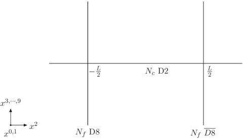
Figure 1: The brane configuration consists of D2, D8 and $\overline{D8}$ branes

In this brane configuration, the low energy effective theory is obtained from the 2-2, 8-8, $\bar{8}$-$\bar{8}$, 8-$\bar{8}$, 2-8 and 2-$\bar{8}$ open strings. In the intersectional dimensions, as analyzed in [11], all the massless modes(quarks $q_{L}$ and $q_{R}$, gauge field $A_{\mu}$) and their transformations under the gauge symmetries can be listed in the following table 1.

field	SO(1,1)	SO(8)	$U(N_{c})\times U(N_{f})_{L}\times U(N_{f})_{R}$
$A_{\mu}$	2	1	(adj, 1, 1 )
$q_{L}$	$1_{+}$	1	$(N_{c},N_{f},1)$
$q_{R}$	$1_{-}$	1	$(N_{c},1,N_{f})$

Table 1: The massless degrees of freedom on the intersection of this brane configuration

The low energy theory on the worldvolume of the D2-branes is a three dimensional $U(N_{c})$ gauge theory with the gauge coupling constant $g_{3}^{2}=g_{s}/l_{s}$. Under the limit, $g_{3}^{2}$ fixed and $\alpha^{\prime}\rightarrow 0$, this theory decouples from the bulk physics since the ten dimensional Newton constant goes to zero. The ’t Hooft coupling constant can be defined as $\lambda=g_{3}^{2}N_{c}/4\pi=g_{s}N_{c}/4\pi l_{s}$. Now we analyze the coupling constant parameter space. As in [20], we introduce an energy scale $U\equiv r/\alpha^{\prime}$, at this energy scale, the effective dimensionless coupling constant in the three dimensional gauge theory is $g^{2}_{eff}\approx\lambda/U$. If $g_{eff}^{2}\gg 1$, the theory will be strong coupled, however, on the other side, the perturbative analysis is valid. Here, the energy scale is the distance $L$ between D8 and $\bar{D8}$ brane in the unit $\alpha^{\prime}=1$. In the regime

$$l_{s}\ll L\ll\frac{1}{\lambda},$$ (2.2)

since the distance scale $L$ is much larger than the string scale $l_{s}$, stringy effects can be neglected. The effective coupling constant $g^{2}_{eff}\approx\lambda L\ll 1$, hence the coupling is weak and the perturbative calculation can be trusted. We can use the perturbative theory to describe the dynamics of quarks $q_{L}$ and $q_{R}$. In [11], we find the low energy effective theory is the non-local Gross-Neveu (GN) model.

If $L\rightarrow\infty$, the $g^{2}_{eff}\rightarrow\infty$, which means the interaction between the left-hand quarks and the right-hand quarks becomes strong with increasing distance $L$. However, if we let $L\rightarrow 0$, the effective coupling constant $g^{2}_{eff}\rightarrow 0$. When the ’t Hooft coupling increases into the regime

$$l_{s}\ll\frac{1}{\lambda}\ll L,~{}~{}~{}~{}~{}\frac{1}{\lambda}\ll l_{s}\ll L,$$ (2.3)

the interaction between $q_{L}$ and $q_{R}$ becomes strong. We can’t use the above perturbative method to perform such a calculation, instead in this regime we can use the SUGRA/Born-Infeld approximation to study the low energy dynamics of the brane system.

The near-horizon geometry of the $N_{c}$ D2-branes is given by

$$\begin{array}[]{lll}&ds^{2}=\left(\frac{U}{R}\right)^{5/2}\left(\eta_{\mu\nu}dx^{\mu}dx^{\nu}+\left(dx^{2}\right)^{2}\right)+\left(\frac{R}{U}\right)^{5/2}\left(\left(dU\right)^{2}+\left(U\right)^{2}d\Omega_{6}^{2}\right)\\ &e^{\phi}=g_{s}\frac{R^{5/4}}{U^{5/4}},~{}~{}~{}~{}~{}C_{012}=-\frac{1}{2}\left(\frac{U^{5}}{R^{5}}-1\right),~{}~{}~{}~{}~{}R^{5}=6\pi^{2}g_{s}N_{c}=6\pi g_{3}^{2}N_{c}\end{array}$$ (2.6)

where $\Omega_{6}$ is the angular direction in $(3456789)$ and $U=r/\alpha^{\prime}$ with transverse radial coordinate $r$. Then we introduce a D8-brane to probe the geometry (2.6) (Since the gauge field on the D8 brane isn’t turned on, the results of the $N_{f}$ coincident D8-branes case is same. In the next section, we will turn on the fluctuation of the gauge field on the D8 branes). The embedding of the D8-brane forms a curve $U=U(x^{2})$ in the $(U,x^{2})$ plane, whose shape is determined by the equations of motion that follows from the DBI (Dirac-Born-Infeld) action. In the background (2.6), the induced metric on the D8-brane is

$$ds^{2}=\left(\frac{U}{R}\right)^{5/2}\eta_{\mu\nu}dx^{\mu}dx^{\nu}+\frac{R^{5/2}}{U^{1/2}}d\Omega_{6}^{2}+\left(\left(\frac{U}{R}\right)^{5/2}\left(\frac{\partial x^{2}}{\partial U}\right)^{2}+\left(\frac{R}{U}\right)^{5/2}\right)dU^{2}.$$ (2.7)

The DBI action for D8-brane is

$$S_{D8}\sim\int dx^{2}U^{7/2}\sqrt{{1+\left(\frac{R}{U}\right)^{5}}U^{\prime 2}},$$ (2.8)

where the $U^{\prime}=dU/dx^{2}$. From the equation (2.8), the equation of motion can be obtained

$$\frac{d}{dx^{2}}\left(\frac{U^{7/2}}{\sqrt{1+\left({\frac{R}{U}}\right)^{5}U^{\prime 2}}}\right)=0.$$ (2.9)

Then we can get the first order differential equation

$$\frac{U^{7/2}}{\sqrt{1+\left({\frac{R}{U}}\right)^{5}U^{\prime 2}}}=U_{0}^{7/2}.$$ (2.10)

The solution $U(x^{2})$ of (2.10) is a curve in the (U, $x^{2}$) plane, which is symmetric under the reflection $x^{2}\rightarrow-x^{2}$. We choose the following boundary conditions: If the $U\rightarrow\infty$, then $x^{2}=\pm\frac{L}{2}$, and at $x^{2}=0$ the $U$ is equal to $U_{0}$. Thus, the solution $x^{2}(U)$ can be obtained as the integral form

$$x^{2}(U)=\int_{U_{0}}^{U}\frac{dU}{\left(\frac{U}{R}\right)^{5/2}\sqrt{\left(\frac{U^{7}}{U_{0}^{7}}-1\right)}}.$$ (2.11)

Under the approximation $U/U_{0}\gg 1$, the curve in the (U, $x^{2}$) plane can be obtained

$$x^{2}(U)=\frac{R^{5/2}}{7U_{0}^{3/2}}\left(B(\frac{5}{7},\frac{1}{2})-B(\left(\frac{U_{0}}{U}\right)^{7},\frac{5}{7},\frac{1}{2})\right).$$ (2.12)

From equation (2.12), we know the asymptotic value $L/2=x^{2}(\infty)=\frac{R^{5/2}}{7U_{0}^{3/2}}B(\frac{5}{7},\frac{1}{2})$. At small $U/U_{0}$, i.e the large $U$, the form of curve $U(x^{2})$ obeys the equation

$$U^{5}=\frac{R^{5/2}U_{0}^{7/2}}{5\left(L/2-x^{2}(U)\right)}.$$ (2.13)

Since the symmetry $x^{2}\rightarrow-x^{2}$, the part of the D-brane at $x^{2}<0$ is determined by $U(x^{2})=U(-x^{2})$. The full D8-brane flow can be determined in the background (2.6) and is shown in fig. 2

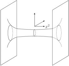
Figure 2: The $N_{f}$ D8 and $\overline{D8}$ branes will be connected in the background (2.6).

In the classical case, we have discussed that the $N_{f}$ D8 and $N_{f}$ $\overline{D8}$-branes in this brane configuration sit at $x^{2}=-\frac{L}{2}$ and $x^{2}=\frac{L}{2}$ respectively, and are separated by a distance $L$. Hence the chiral symmetry $U(N_{f})_{L}\times U(N_{f})_{R}$ is not broken. But due to the quantum effects, the $N_{f}$ D8-branes and $N_{f}$ $\overline{D8}$-branes are joined into a single D8-branes by a wormhole and the chiral symmetry $U(N_{f})_{L}\times U(N_{f})_{R}$ is dynamically broken to a $U(N_{f})_{diag}$. We can compare the energy density of these two configuration to see which one is preferred. The energy density difference of the two configurations is given by

$$\bigtriangleup E\equiv E_{straight}-E_{curved}$$

$$\sim\int_{0}^{U_{0}}(U-0)dU+\int_{U_{0}}^{\infty}\left(U-U(1-\frac{U_{0}^{7}}{U^{7}})^{-1/2}\right)dU\approx 0.4U_{0}^{2}.$$ (2.14)

We find the energy density difference $\bigtriangleup E$ is positive. This result means that the configuration connected by the wormhole is preferred and the chiral symmetry is broken.

In order for the supergravity method to be reliable in this regime, two conditions must be satisfied. One is $e^{\phi}\ll 1$, and the other is that scalar curvature satisfies $\alpha^{\prime}R\ll 1$. Therefore the ’t Hooft coupling constant must be satisfied

$$U\ll\lambda$$ (2.15)

which is extended by the eleven-dimensional SUGRA. From (2.12), we have $U_{0}^{3}\sim\lambda/L^{2}$. Actually, $U_{0}$ obviously satisfies the condition (2.15). Fixing $L$ and increasing $\lambda$ will push $U_{0}$ further into the region of validity of supergravity. In the opposite direction, decreasing $\lambda$ will make $U_{0}$ become smaller, and when $L\simeq\frac{1}{\lambda}$ the curvature at $U_{0}$ becomes of order one and the supergravity description breaks down. By continuing to decrease $\lambda$ into the region $L\ll\frac{1}{\lambda}$, the coupling becomes weak and the perturbative description is valid.

3 Nambu-Goldstone boson

In the last section, we have given a review of the chiral symmetry breaking in the holographic model from the intersecting D-brane configuration D8/$\overline{D8}$/D2. Now, in the following, we investigate the Nambu-Goldstone bosons associated with this chiral symmetry breaking. Following the method in [8, 10, 13], we can turn on the fluctuations of the gauge field on the worldvolume of the flavor D8-branes. The gauge field on this probe D8-brane is labeled by $A_{M}$, ($M=0,~{}1,~{}U,~{}d\Omega_{6}$). Since we are mainly interested in the $SO(7)$ singlet states, we can set the components $A_{\alpha}$ of the gauge field on the $S^{6}$ to vanish and the other components $A_{\mu}(\mu=0,1)$, $A_{U}$ to be independent of the coordinates on the sphere $S^{6}$. Then, for the $U(1)$ case, the effective action of the D8-brane in the background (2.6) is

$$S = S_{DBI}+S_{cs}$$

$$S_{DBI} = -T_{8}\int d^{9}xe^{-\phi}\sqrt{-\det(g_{MN}+2\pi F_{MN})}$$

$$S_{cs} = T_{8}\int(C_{3}+C_{5})\wedge e^{2\pi F_{2}}.$$ (3.1)

The first term in the CS (Chern-Simons) terms can be omitted due to the three powers of the gauge field strength $F_{2}$. However, to the second term, which has the same order as the DBI action part, hence, we can throw it away. We choose that the Hodge dual of the RR (Ramond-Ramond) field $F_{4}$ is $F_{6}=\frac{N_{c}}{V_{S^{6}}}\epsilon_{6}$, where the $V_{S^{6}}$, $\epsilon_{6}$ are the volume of the sphere $S^{6}$ volume form of the sphere $S^{6}$ respectively. Thus, the contribution from the CS-term is

$$S_{cs} = 4\pi^{2}T_{8}\int C_{5}\wedge F_{2}\wedge F_{2}+O(F_{2}^{3})$$ (3.2)

$$= 4\pi^{2}N_{c}T_{8}\int A\wedge F_{2}+O(F_{2}^{3})$$

After expanding the field strength and omitting the high order terms, we can obtain the action

$$S=-(2\pi)^{2}T_{8}V_{S^{6}}\int d^{2}xdUe^{-\phi}\sqrt{-\det g_{MN}}[\frac{1}{4}F_{MN}F^{MN}]+4\pi^{2}N_{c}T_{8}\int A\wedge F_{2}.$$ (3.3)

Now we can substitute the induced metric of the D8-brane into the equation (2.10), the above equation becomes

$$S=-\frac{(2\pi)^{2}T_{8}V_{S^{6}}}{g_{s}}\int d^{2}xdU\left[\frac{1}{4}G(U)F_{\mu\nu}F^{\mu\nu}+\frac{1}{2}H(U)F_{\mu U}F^{\mu}_{U}\right]$$

$$+2\pi^{2}N_{c}T_{8}\int d^{2}xdU\epsilon^{\mu\nu}\left[A_{U}F_{\mu\nu}+2A_{\mu}F_{\nu U}\right]$$ (3.4)

where the indices are contracted under the Minkowski metric $\eta_{\mu\nu}$, and the $G(U)$, $H(U)$ are defined in the following equations

$$G(U) = \frac{R^{10}}{U^{1/2}\sqrt{U^{7}-U_{0}^{7}}},$$

$$H(U) = \frac{R^{5}\sqrt{U^{7}-U_{0}^{7}}}{U^{5/2}}.$$ (3.5)

We can expand the gauge field components $A_{\mu}$ and $A_{U}$ in terms of the complete basis $\psi_{n}(U)$ and $\phi_{n}(U)$ as follows

$$A_{\mu}(x,U)=\sum_{n}B_{\mu}^{n}(x)\psi_{n}(U),$$

$$A_{U}(x,U)=\sum_{n}\varphi^{n}(x)\phi_{n}(U).$$ (3.6)

Then the gauge field strength will be

$$F_{\mu\nu}(x,U) = \sum_{n}\left(\partial_{\mu}B^{n}_{\nu}(x)-\partial_{\nu}B^{n}_{\mu}(x)\right)\psi_{n}(U)$$ (3.7)

$$\equiv \sum_{n=0}^{\infty}B_{\mu\nu}^{n}(x)\psi_{n}(U),$$

$$F_{\mu U}(x,U) = \sum_{n}\left(\partial_{\mu}\varphi^{n}(x)\phi_{n}(U)-B^{n}_{\mu}(x)\dot{\psi}_{n}(U)\right)$$ (3.8)

where the $\dot{\psi}_{n}(U)$ denotes the $\partial_{U}\psi_{n}(U)$. Inserting the above two equations into the action (3.4), we get

$$S = -\frac{(2\pi)^{2}T_{8}V_{S^{6}}}{g_{s}}\int d^{2}xdU\sum_{m,n}\left[\frac{1}{4}G(U)B_{\mu\nu}^{m}B^{n\mu\nu}\psi_{m}\psi_{n}\right.$$ (3.9)

$$\left.+\frac{1}{2}H(U)\left(\partial_{\mu}\varphi^{m}\partial^{\mu}\varphi^{n}\phi_{m}\phi_{n}+B_{\mu}^{m}B^{n\mu}\dot{\psi}_{m}\dot{\psi}_{n}-2\partial_{\mu}\varphi^{m}B^{n\mu}\phi_{m}\dot{\psi}_{n}\right)\right]$$

$$+2\pi^{2}N_{c}T_{8}\int d^{2}xdU\epsilon^{\mu\nu}\sum_{m,n}\left[B^{m}_{\mu\nu}\varphi^{n}\psi_{m}\phi_{n}\right.$$

$$\left.+2(B^{m}_{\mu}\partial_{\nu}\varphi^{n}\psi_{m}\phi_{n}-B^{m}_{\mu}B^{n}_{\nu}\psi_{m}\dot{\psi}_{n})\right].$$

We set the basis $\psi_{n}(U)$ to satisfy the following normalization condition

$$\frac{(2\pi)^{2}T_{8}V_{S^{6}}}{g_{s}}\int dUG(U)\psi_{n}(U)\psi_{m}(U)=\delta_{mn}.$$ (3.10)

Then the first term in the equation (3.9) will become

$$-\sum_{n=1}\int d^{2}x\frac{1}{4}B_{\mu\nu}^{n}B^{n\mu\nu}$$ (3.11)

which are the kinetic terms for the gauge field $B_{\mu}^{n}$ in two dimensions. If we choose the field $\psi_{n}(U)$ $(n\geq 1)$ to satisfy the equation

$$\frac{1}{G(U)}\partial_{U}[H(U)\dot{\psi}_{n}(U)]=-m_{n}^{2}\psi_{n}(U),$$ (3.12)

then $\dot{\psi}_{n}(U)$ satisfies the normalization condition

$$\frac{(2\pi)^{2}T_{8}V_{S^{6}}}{g_{s}}\int dUH(U)\dot{\psi}_{n}(U)\dot{\psi}_{m}(U)=m_{n}^{2}\delta_{mn}.$$ (3.13)

From the equation (3.9), we obtain the mass term for the gauge fields $B_{\mu}^{n}$, it is

$$-\sum_{n=1}\int d^{2}x\frac{1}{2}m_{n}^{2}B_{\mu}^{n}B^{n\mu}$$ (3.14)

Thus, for the fields $B_{\mu}^{n}$ $(n\geq 1)$, summing the equation (3.11) and (3.14), we get the action for these massive gauge fields in two dimensions

$$S_{B}=-\sum_{n=1}\int d^{2}x\left[\frac{1}{4}B_{\mu\nu}^{n}B^{n\mu\nu}+\frac{1}{2}m_{n}^{2}B_{\mu}^{n}B^{n\mu}\right].$$ (3.15)

For the complete basis $\phi_{n}(U)$, we impose the normalization condition

$$\frac{(2\pi)^{2}T_{8}V_{S^{6}}}{g_{s}}\int dUH(U)\phi_{n}(U)\phi_{m}(U)=\delta_{mn}.$$ (3.16)

From the equation (3.13), we let $\phi_{n}=m_{n}^{-1}\dot{\psi}_{n}$ for the $n\geq 1$ cases. For the zero mode $\phi_{0}$, if we choose $\phi_{0}=C/H(U)$, then

$$\frac{(2\pi)^{2}T_{8}V_{S^{6}}}{g_{s}}\int dUH(U)\phi_{0}(U)\phi_{m}(U)=\frac{(2\pi)^{2}T_{8}V_{S^{6}}}{m_{n}g_{s}}\int dUH(U)\phi_{0}\dot{\psi}_{m}\sim\int dU\dot{\psi}_{n}=0.$$ (3.17)

Hence the zero mode $\phi_{0}$ is orthogonal to the basis $\phi_{n}$ and $\dot{\psi}_{n}$ for all $n\geq 1$. The normalization condition of the zero mode $\phi_{0}(U)$ is

$$\frac{(2\pi)^{2}T_{8}V_{S^{6}}}{g_{s}}\int dUH(U)\phi_{0}(U)\phi_{0}(U)=\frac{(2\pi)^{2}T_{8}V_{S^{6}}C^{2}}{g_{s}}\int dUH^{-1}.$$ (3.18)

Due to the $H=\frac{R^{5}\sqrt{U^{7}-U_{0}^{7}}}{U^{5/2}}$, then the integral $\int dUH^{-1}$ will be logarithmic divergence. It means that the zero mode $\phi_{0}$ can’t be normalized. While, due to the integral $\int dUG(U)\psi_{0}\psi_{0}$ is convergent, another zero constant mode $\psi_{0}(U)$ is normalized. All these results are same as the corresponding ones in [10], but are different from the ones in [8].

And using the definition

$$2\pi^{2}N_{c}T_{8}\int dU\psi_{m}\dot{\psi}_{n}=M_{mn},~{}~{}2\pi^{2}N_{c}T_{8}\int dU\phi_{0}\psi_{n}=M_{m}.$$ (3.19)

Then the full fluctuation action is

$$S = -\int d^{2}x\left[\frac{1}{4}B_{\mu\nu}^{0}B^{0\mu\nu}+\sum_{n=1}\left(\frac{1}{2}\partial_{\mu}\varphi^{n}\partial^{\mu}\varphi^{n}+\frac{1}{4}B_{\mu\nu}^{n}B^{n\mu\nu}+\frac{1}{2}m_{n}^{2}B_{\mu}^{n}B^{n\mu}\right.\right.$$ (3.20)

$$\left.\left.-m_{n}\partial_{\mu}\varphi^{n}B^{n\mu}\right)\right]+\sum_{m,n=1}\int d^{2}x\epsilon^{\mu\nu}\left[M_{m}(\varphi^{0}B^{m}_{\mu\nu}+2B^{m}_{\mu}\partial_{\nu}\varphi^{0})\right.$$

$$\left.+M_{mn}(m_{n}^{-1}B^{m}_{\mu\nu}\varphi^{n}-2B^{m}_{\mu}(B^{n}_{\nu}-m_{n}^{-1}\partial_{\nu}\varphi^{m}))\right].$$

Through the gauge transformation

$$B^{n}_{\mu}\rightarrow B^{n}_{\mu}-m_{n}^{-1}\partial_{\mu}\varphi^{n},$$ (3.21)

the $\partial_{\mu}\varphi^{n}$ can be absorbed into the field $B_{\mu}^{n}$ in the first line of the equation (3.20). Hence the final action is

$$S = -\int d^{2}x\left[\frac{1}{4}B_{\mu\nu}^{0}B^{0\mu\nu}+\sum_{n=1}\left(\frac{1}{4}B_{\mu\nu}^{n}B^{n\mu\nu}+\frac{1}{2}m_{n}^{2}B_{\mu}^{n}B^{n\mu}\right)\right]$$ (3.22)

$$+\sum_{m,n=1}\int d^{2}x\epsilon^{\mu\nu}\left[M_{n}(\varphi^{0}B^{n}_{\mu\nu}+2(B^{n}_{\mu}+m_{n}^{-1}\partial_{\mu}\varphi^{n})\partial_{\nu}\varphi^{0})-2M_{mn}B^{m}_{\mu}B^{n}_{\nu})\right].$$

In the above equation, there exists some coupling terms between the zero mode $\varphi_{0}$ and other modes $\epsilon^{\mu\nu}M_{n}[\varphi^{0}B^{n}_{\mu\nu}+2(B^{n}_{\mu}+m_{n}^{-1}\partial_{\mu}\varphi^{n})\partial_{\nu}\varphi^{0}]$. And since the $\phi_{0}(U)$ is not normalized, the equation (3.22) doesn’t have the kinetic term of the mode $\varphi^{0}$. Thus, we can’t regard the $\varphi^{0}$ as a massless field, and can’t be taken as the Nambu-Goldstone boson associated with the chiral symmetry breaking.

As in [8], we can change inot the $A_{U}=0$ gauge, which can be chosen due to the gauge transformation

$$A_{M}\rightarrow A_{M}-\partial_{M}\Lambda$$ (3.23)

with the $\Lambda=\sum_{n=1}m_{n}^{-1}\varphi^{n}\psi_{n}(U)$. Then after substituting these into the equation (3.4), we can get the action is

$$S = -\int d^{2}x\left[\frac{1}{4}B^{0}_{\mu\nu}B^{0\mu\nu}+\sum_{n=1}\left(\frac{1}{4}B^{n}_{\mu\nu}B^{n\mu\nu}+\frac{1}{2}m_{n}^{2}B^{n}_{\mu}B^{n\nu}\right)\right]$$ (3.24)

$$-2\int d^{2}x\sum_{m,n}\epsilon^{\mu\nu}M_{mn}B^{n}_{\mu}B^{m}_{\nu}.$$

This action is same as the equation (3.22) after throwing out the zero mode $\varphi_{0}$ due to the non-normalization of $\phi_{0}$. And this result is also same as the one in the [10, 13]. As the same arguments in [10], it is difficult to diagonalize the infinite-dimensional matrix, but generally the mass eigenvalues of the meson fields $B^{n}_{\mu}$ does not vanish.

Thus, for the D8/$\overline{D8}/D2$ brane system, after the above analysis, we doesn’t find the NG-boson associated with the $U(1)$ chiral symmetry breaking. The reason may be the NG boson will not be visible in the analysis of the near horizon geometry because these degrees lives a far distance from the D2 brane [10].

In order to investigate the chiral symmetry $U(N_{f})_{L}\times U(N_{f})_{R}$ broken to $U(N_{f})_{diag}$, we need generalize to the $N_{f}$ flavor D8 branes case. For the multi-flavors to probe the near horizon background (2.6), we need use the non-Abelian DBI action to describe the dynamics of the D8 branes [21]. Using the same ansantz for the gauge field as the $U(1)$ case and omitting the higher order terms of the field strength, the action of the gauge field on the D8-branes in the background of solution (2.12) reads

$$S = -\frac{(2\pi)^{2}T_{8}V_{S^{6}}}{g_{s}}\int d^{2}xdU\mathop{\rm Tr}\nolimits\left[\frac{1}{4}G(U)F_{\mu\nu}F^{\mu\nu}+\frac{1}{2}H(U)F_{\mu U}F^{\mu}_{U}\right]$$ (3.25)

$$+4\pi^{2}N_{c}T_{8}\mathop{\rm Tr}\nolimits\int\left(A\wedge dA+\frac{2}{3}A\wedge A\wedge A\right)$$

where the field strength is $F_{\mu\nu}=\partial_{\mu}A_{\nu}-\partial_{\nu}A_{\mu}+[A_{\mu},A_{\nu}]$, and the trace $\mathop{\rm Tr}\nolimits{T^{a}T^{b}}=N_{f}\delta^{ab}$ under the gauge group $U(N_{f})$.

We then expand the gauge field in the complete basis $\psi_{n}(U)$ and $\phi_{n}(U)$ as the same in the $U(1)$ case, except where the modes $B_{\mu}^{n}(x)$ and $\varphi^{n}(x)$ transform under the adjoint representation of the gauge group $U(N_{f})$. Then using the normalization conditions as same in the $U(1)$ case and the following definitions

$$\frac{(2\pi)^{2}T_{8}V_{S^{6}}}{g_{s}}\int dUG(U)\psi_{n}(U)\psi_{m}(U)\psi_{k}(U)=A_{nmk},$$ (3.26)

$$\frac{(2\pi)^{2}T_{8}V_{S^{6}}}{g_{s}}\int dUG(U)\psi_{n}(U)\psi_{m}(U)\psi_{k}(U)\psi_{l}(U)=B_{nmkl},$$ (3.27)

$$\frac{(2\pi)^{2}T_{8}V_{S^{6}}}{g_{s}}\int dUH(U)\psi_{n}(U)\phi_{m}(U)\phi_{k}(U)=C_{nmk},$$ (3.28)

$$\frac{(2\pi)^{2}T_{8}V_{S^{6}}}{g_{s}}\int dUH(U)\psi_{n}(U)\dot{\psi}_{m}(U)\phi_{k}(U)=D_{nmk},$$ (3.29)

$$\frac{(2\pi)^{2}T_{8}V_{S^{6}}}{g_{s}}\int dUH(U)\psi_{n}(U)\psi_{m}(U)\phi_{k}(U)\phi_{l}(U)=E_{nmkl},$$ (3.30)

we can get all the terms of the $F_{\mu\nu}F^{\mu\nu}$ and $F_{\mu U}F^{\mu U}$ in the first line of the action (3.25) as follows

$$-\frac{1}{4}\mathop{\rm Tr}\nolimits\left[\sum_{n=0}B^{n}_{\mu\nu}B^{n\mu\nu}+2\sum_{n,m,k=0}A_{nmk}B^{n}_{\mu\nu}[B^{m\mu},B^{k\nu}]\right.$$

$$\left.~{}~{}~{}~{}+\sum_{n,m,k,l=0}B_{nmkl}[B_{\mu}^{m},B_{\nu}^{n}][B^{k\mu},B^{l\nu}]\right]$$

$$-\frac{1}{2}\mathop{\rm Tr}\nolimits\left[\sum_{n=1}\left(\partial_{\mu}\varphi^{n}\partial^{\mu}\varphi^{n}-2m_{n}\partial_{\mu}\varphi^{n}B^{n\mu}+m_{n}^{2}B^{n}_{\mu}B^{n\mu}\right)\right.$$

$$\left.+2\sum_{n,k\geq 1;m=0}\left(C_{mnk}\partial_{\mu}\varphi^{n}-D_{mnk}B_{\mu}^{n}\right)[B^{m\mu},\varphi^{k}]\right.$$

$$\left.~{}~{}~{}~{}~{}~{}+\sum_{n,l\geq 1;m,k=0}E_{mknl}[B^{m}_{\mu},\varphi^{n}][B^{k\mu},\varphi^{l}]\right]$$ (3.31)

where the $B^{n}_{\mu\nu}=\partial_{\mu}B^{n}_{\mu}-\partial_{\nu}B^{n}_{\mu}$. For the $N_{f}=1$ case, since the constants $A_{nmk}$, $B_{nmkl}$, $C_{nmk}$, $D_{nmk}$, $E_{nmkl}$ all vanish, the above equations will reduce to equation (3.22) through the gauge transformation (3.21). However, if $N_{f}\neq 1$, the constants $A_{nmk},B_{nmkl},C_{nmk},D_{nmk}$ and $E_{nmkl}$ cannot vanish all together.

The second line, setting to be $\chi$, in the action (3.25) contributed from the CS term, after substituting the expansion of the gauge field, reads

$$\chi = 2\pi^{2}N_{c}T_{8}\mathop{\rm Tr}\nolimits\int d^{2}xdU\epsilon^{\mu\nu}\left(A_{U}(\partial_{\mu}A_{\nu}-\partial_{\nu}A_{\mu})+\frac{4}{3}A_{\mu}A_{\nu}A_{U}\right)$$ (3.32)

$$= 2\pi^{2}N_{c}T_{8}\mathop{\rm Tr}\nolimits\int d^{2}xdU\epsilon^{\mu\nu}\sum_{m,n,k}\left[B^{m}_{\mu\nu}\varphi^{n}\psi_{m}\phi_{n}\right.$$

$$\left.+2(B^{m}_{\mu}\partial_{\nu}\varphi^{n}\psi_{m}\phi_{n}-B^{m}_{\mu}B^{n}_{\nu}\psi_{m}\dot{\psi}_{n})+\frac{4}{3}B^{n}_{\mu}B^{m}_{\nu}\varphi^{k}\psi_{n}\psi_{m}\phi_{k}\right].$$

Using the same definition as the equation (3.19), and the condition (3.30), we can get

$$\chi = \sum_{m,n=1}\mathop{\rm Tr}\nolimits\int d^{2}x\epsilon^{\mu\nu}\left[M_{m}(\varphi^{0}B^{m}_{\mu\nu}+2B^{m}_{\mu}\partial_{\nu}\varphi^{0})\right.$$ (3.33)

$$\left.+M_{mn}(m_{n}^{-1}B^{m}_{\mu\nu}\varphi^{n}-2B^{m}_{\mu}(B^{n}_{\nu}-m_{n}^{-1}\partial_{\nu}\varphi^{m}))\right]$$

$$+\frac{2N_{c}g_{s}C}{3V_{S^{6}}}\sum_{n,m,k=0}\mathop{\rm Tr}\nolimits\int d^{2}xE_{nmk0}\epsilon^{\mu\nu}B^{n}_{\mu}B^{m}_{\nu}\varphi^{k}.$$

From the equation (3.31) and (3.33), we can see there doesn’t exists the kinetic term of the zero mode $\varphi_{0}$ due to the non-normalization, and the modes $\varphi^{0}$ are not massless NG bosons. Thus, through the analysis of the gauge field fluctuation on the $N_{f}$ D8 branes, we don’t find the $N_{f}^{2}$ massless NG bosons in the spectrum corresponding to this chiral symmetry breaking.

4 Conclusions

In [11], the intersecting brane configuration $D8/\overline{D8}/D2$ was constructed in IIA string theory. The low energy theory on this brane configuration can be analyzed using two methods. In the weak coupling regime, the perturbative method is reliable and the low energy theory is a nonlocal generalization of the GN model which dynamically breaks the chiral flavor symmetry $U(N_{f})_{L}\times U(N_{f})_{R}$ at large $N_{c}$ and finite $N_{f}$. However, in the strong coupling region, we can use the supergravity approximation to describe the low energy dynamics of the brane system. In the near horizon geometry of $N_{c}$ D2 branes, we find that the connected shape of $N_{f}$ D8 and $\overline{D8}$ through a throat in fig. 2 is preferred to the separated case of $N_{f}$ D8 and $\overline{D8}$ in fig. 1 from equation (2.14). In the connected case of $N_{f}$ D8 and $\overline{D8}$ branes, the chiral symmetry $U(N_{f})_{L}\times U(N_{f})_{R}$ is broken to the gauge group $U(N_{f})_{diag}$. Thus, totally $N_{f}^{2}$ generators of the symmetry $U(N_{f})_{L}\times U(N_{f})_{R}$ are broken in this process.

Associated with this global symmetry breaking, there must exist some massless Nambu-Goldstone bosons in the spectrum. In the section 3, we have given a detailed analysis of the fluctuation of the gauge field on the flavor D8 branes. For the $U(1)$ case, since the zero mode $\phi_{0}(U)$ is not normalized, we can’t find one massless Nambu-Goldstone boson in the spectrum which is corresponding to the chiral symmetry breaking. For the $U(N_{f})$ case, we already know that the chiral symmetry $U(N_{f})_{L}\times U(N_{f})_{R}$ is be broken to $U(N_{f})_{diag}$ in section 2. However, we still don’t see the NG modes in the spectrum with the same reason as in the $U(1)$ case. So the results in this two dimensional model are different from the ones in [8], but are consistent with [10, 13, 14].

It may be interesting to generalize to other holographic models, constructed from brane configurations such as Dp/$\overline{Dp}$/D2 $(p=4,6)$. The intersecting region of these brane configurations is still two dimensional, $(x^{0},x^{1})$. In these intersecting dimensions, in the weak coupling regime, the low energy physics can be described by the effective field theory. In the strong coupling regime, the supergravity method can be used to analyze the physics as in the D8/$\overline{D8}$/D2 brane configuration [11]. In the near horizon geometry of $N_{c}$ D2 branes, we find that the flavor Dp and $\overline{Dp}$ $(p=4,6)$ branes connect at some critical point, which means the chiral symmetry is broken. Thus, for these holographic brane models, one can use the methods in this paper to analyze the chiral symmetry breaking pattern, and to see whether the NG modes exist.

References

[1]
J. Maldacena, “The Large N limit of superconformal field theories
and supergravity,” Adv. Theor. Math. Phys. 2: 231-252, 1998; Int.
J. Theor. Phys. 38: 1113-1133, 1999 [arXiv: hep-th/9711200];
S. S. Gubser, I. R. Klebnov and A. M. Polyakov, “Gauge Theory
Correlators from Noncritical String Theory,” Phys. Lett. B428:
105-114, 1998 [arXiv: hep-th/9802109]; E. Witten, “Anti-de Sitter
Space and Holography,” Adv. Theor. Math. Phys. 2: 253-291, 1998
[arXiv: hep-th/9802150].
[2]
J. Polchinski and M. J. Strassler, “The String dual of a confining
four-dimensional gauge theory,” arXiv: hep-th/0003136.
[3]
I. R. Klebanov and M. J. Strassler, “Supergravity and a Confining
Guage Theory: Duality Cascades and SB-Resolution of Naked
Singularties,” J. High Energy Phys. 0008, 052 (2000) [arXiv:
hep-th/0007191].
[4]
J. M. Maldacena and C. Nunez, “Towards the Large N Limit of Pure
N=1 Super Yang-Mills,” Phys. Rev. Lett. 86, 588 (2001) [arXiv:
hep-th/0008001].
[5]
E. Witten, “Anti-de Sitter space, thermal phase transition, and
confinement in gauge theories,” Adv. Theor. Math. Phys. 2 (1998)
505 [arXiv: hep-th/9803131].
[6]
A. Karch and E. Katz, “Adding Flavor to ads/cft,” J. High Energy
Phys. 06 (2002) 043 [arXiv: hep-th/0205236].
[7]
M. Kruczenski, D. Mateos, R. C. Myers and D. J. Winters, “ Meson
spectroscopy in AdS/CFT with flavor,” JHEP 0307: 049, 2003 [arXiv:
hep-th/0304032]; “Towards a Holographic Dual of Large-Nc QCD,” J.
High Energy Phys. 05 (2004) 041 [arXiv: hep-th/0311270].
[8]
T. Sakai and S. Sugimoto, “Low Energy Hadron Physics in Holographic
QCD,” Prog. Theor. Phys. 113: 843-882, 2005 [arXiv:
hep-th/0412141]; “More on A Holographic QCD,” Prog. Theor. Phys.
114: 1083-1118, 2006 [arXiv: hep-th/0507073].
[9]
E. Antonyan, J. A. Harvey, S. Jensen and D. Kutasov, “NJL and QCD
from String Theory,” arXiv: hep-th/0604017.
[10]
E. Antonyan, J. A. Harvey and D. Kutasov, “The Gross-Neveu Model
from String Theory,” arXiv: hep-th/0608177; “Chiral symmetry
breaking from intersecting D-branes,” arXiv: hep-th/0608149;
[11]
Y. h. Gao, W. s. Xu and D. f. Zeng, “NGN, QCD2 and chiral phase
transition from string theory”, JHEP 0608, 018 (2006) [arXiv:
hep-th/0605138].
[12]
A. Basu and A. Maharana, “Generalized Gross-Neveu models and
chiral symmetry breaking from string theory,” Phys. Rev. D75:
065005, 2007 [arXiv: hep-th/0610087].
[13]
D. Gepner and S. S. Pal, “Chiral symmetry breaking and
restoration from holography,” [arXiv: hep-th/0608229].
[14]
L. Grisa, “Delocalization from anomaly inflow and intersecting
brane dynamics,” JHEP 0703, 017 (2007)
[arXiv:hep-th/0611331].
[15]
J. Babington, J. Erdmenger, N. J. Evans, Z. Guralnik and I. Kirsch,
“Chiral Symmetry Breaking and Pions in Non-supersymmetric
Gauge/Gravity Duals,” Phys. Rev. D69, 066007 (2004) [arXiv:
hep-th/0306018]; N. J. Evans and J. P. Shock, “Chiral dynamics from
AdS space,” Phys. Rev. D 70: 046002, 2004 [arXiv: hep-th/0403279];
N. J. Evans, J. P. Shock and T. Waterson, “D7 brane embeddings and
chiral symmetry breaking,” JHEP 0503: 005, 2005 [arXiv:
hep-th/0502091].
[16]
O. Aharony, J. Sonnenschein and S. Yankielowicz, “A Holographic
Model of Deconfinement and Chiral Symmetry Restoration,” arXiv:
hep-th/0604161.
[17]
A. Parnachev and D. A. Sahakyan, “Chiral Phase Transition from
String Theory,” Phys. Rev. Lett. 97: 111601, 2006 [arXiv:
hep-th/0604173].
[18]
A. Karch and A. O’Bannon, “Chiral Transition of N=4 Super
Yang-Mills with Flavor on a 3-Sphere,” Phys. Rev. D74: 085033, 2006
[arXiv: hep-th/0605120].
[19]
R. Casero, E. Kiritsis and A. Paredes, “Chiral symmetry breaking as
open string tachyon condensation,” arXiv: hep-th/0702155.
[20]
N. Itzhaki, J. M. Maldacena, J. Sonnenschein and S. Yankielowicz,
“Supergravity and The Large N Limit of Theories With Sixteen
Supercharges,” Phys. Rev. D58: 046004, 1998 [arXiv:
hep-th/9802042].
[21]
R. C. Myers, “Dielectric Brane,” JHEP 9912: 022, 1999 [arXiv:
hep-th/9910053].