Developments in entanglement theory and applications to relevant physical systems

DEVELOPMENTS IN ENTANGLEMENT THEORY AND APPLICATIONS TO RELEVANT PHYSICAL SYSTEMS

Tesis Doctoral realizada por
D. Lucas Lamata Manuel,
y dirigida por el
Dr. D. Juan León García,
Investigador Científico del
Instituto de Matemáticas y Física Fundamental (CSIC)

Madrid, 2007

Committee: I. Cirac, D. Salgado, G. García-Alcaine, M.A. Martin-Delgado, A. Cabello

For this ArXiv reprint, the introduction and conclusions, in Spanish in the initial version submitted to UAM, were translated into English, and some of the preprints and works in preparation were updated in the List of Publications and Bibliography with their published references.

Madrid, April 2007

List of Publications

• Entanglement and Relativistic Quantum Theory

  1. L. Lamata, J. León, and E. Solano, Dynamics of momentum entanglement in lowest-order QED, Phys. Rev. A 73, 012335 (2006).

  2. L. Lamata and J. León, Generation of bipartite spin entanglement via spin-independent scattering, Phys. Rev. A 73, 052322 (2006).

  3. L. Lamata, M. A. Martin-Delgado, and E. Solano, Relativity and Lorentz Invariance of Entanglement Distillability, Phys. Rev. Lett. 97, 250502 (2006).

  4. L. Lamata, J. León, T. Schätz, and E. Solano, Dirac Equation and Quantum Relativistic Effects in a Single Trapped Ion, Submitted to Phys. Rev. Lett., quant-ph/0701208.

• Continuous-variable entanglement

  1. L. Lamata, J. J. García-Ripoll, and J. I. Cirac, How Much Entanglement Can Be Generated between Two Atoms by Detecting Photons?, Phys. Rev. Lett. 98, 010502 (2007).

  2. L. Lamata, J. León, and D. Salgado, Spin entanglement loss by local correlation transfer to the momentum, Phys. Rev. A 73, 052325 (2006).

  3. L. Lamata and J. León, Dealing with entanglement of continuous variables: Schmidt decomposition with discrete sets of orthogonal functions, J. Opt. B: Quantum Semiclass. Opt. 7, 224 (2005).

• Multipartite entanglement

  1. Y. Delgado, L. Lamata, J. León, D. Salgado, and E. Solano, Sequential Quantum Cloning, Phys. Rev. Lett. (in press), quant-ph/0607105 (2006).

  2. L. Lamata, J. León, D. Salgado, and E. Solano, Inductive classification of multipartite entanglement under stochastic local operations and classical communication, Phys. Rev. A 74, 052336 (2006).

  3. L. Lamata, J. León, D. Salgado, and E. Solano, Inductive entanglement classification of four qubits under stochastic local operations and classical communication, Phys. Rev. A 75, 022318 (2007).

Abstract

The non-classical, non-local quantum correlations so-called entanglement, which are possibly the greatest mystery of quantum mechanics, have been proved to be a very useful resource. Entanglement may be used to make exponentially faster computations with a quantum computer than the equivalent ones with a classical computer. Also, it has been shown to introduce advantages in the quantum communication protocols over the classical ones. Moreover, nowadays it is possible to codify provably secure messages through the quantum cryptography protocols (which have a deep relationship with entanglement), in opposition to the classical protocols, which are just conditionally secure.

This Thesis is devoted to the analysis of entanglement in relevant physical systems. Entanglement is the conducting theme of this research, though I do not dedicate to a single topic, but consider a wide scope of physical situations.

I have followed mainly three lines of research for this Thesis, with a series of different works each, which are:

• Entanglement and Relativistic Quantum Theory.

  I show the unbounded entanglement growth appearing in $S$-matrix theory of scattering for incident fermions with sharp momentum distributions, in the context of quantum electrodynamics. I study the possibility of spin entanglement generation through spin-independent scattering of identical particles. I also analyze the properties of Lorentz invariance and relativity of entanglement distillability and separability. I propose the complete simulation of Dirac equation and its remarkable relativistic quantum effects like Zitterbewegung or Klein’s paradox in a single trapped ion.

• Continuous-variable entanglement.

  I demonstrate that an arbitrary, unbounded degree of entanglement may be achieved between two atoms by measurements on the light they emit, when taking into account additional ancillary photons. I detect the spin entanglement loss due to transfer of correlations to the momentum degree of freedom of $s=\frac{1}{2}$ fermions or photons, through local interactions entangling spin and momentum. I also develop a mathematical method for computing analytic approximations of the Schmidt modes of a bipartite amplitude with continuous variables. I study the momentum entanglement generated in the decay of unstable systems and verify that, surprisingly, the asymptotic entanglement is smaller for wider decay widths, related to stronger interactions.

• Multipartite entanglement.

  After a careful analysis of the $1\rightarrow M$ approximate quantum cloning for qubits sequentially implemented, I show that it can be done with just linear resources of the ancilla: the dimension of the ancilla Hilbert space grows linearly with the number of clones, while for arbitrary multiqubit states sequentially generated it would grow exponentially in the number of qubits. This has remarkable experimental interest as it provides a procedure for reducing approximate quantum cloning to sequential two-body interactions, which are the ones experimentally feasible in laboratory. I also propose an inductive scheme for the classification of $N$-partite entanglement, for arbitrary $N$, under stochastic local operations and classical communication, based on the analysis of the coefficient matrix of the pure state in an arbitrary product basis. I give the complete classification of genuine 4-qubit entanglement.

Chapter 1 Introduction

I would not call that one but rather the characteristic trait of quantum mechanics

-Erwin Schrödinger [Sch35]

1.1 Motivation

Quantum computation and quantum information is the field that deals with the information processing and transmission making use of quantum systems. This is a discipline that has begun its development in recent years, and to which a lot of effort is being devoted (for a review of the field, see for example [GMD02, NC00]). Its interest stems from the fact that there are physical tasks regarding information processing and transmission that can be possibly done more efficiently with quantum systems than with the ordinary classical ones. Some examples are the following:

1. Regarding information processing we highlight

   • The factorization of large integer numbers into primes[Sho97].

     This takes a time that grows exponentially in the number of digits $N$ of the integer being factorized with the most powerful classical algorithms known. That is the property in which many classical cryptography systems are based, i.e. public key distribution. With Shor’s algorithm a quantum computer would only use a polynomial time in $N$.

   • Search algorithms [Gro97].

     “Quantum mechanics helps in searching for a needle in a haystack” (L. Grover). With a classical computer it takes a time of order $N$ to find a given item in a disorganized list of size $N$. In a quantum computer it would take a time that grows as $\sqrt{N}$, with Grover’s algorithm.

2. Regarding information transmission, we mention

   • Quantum cryptography [Wie83, BBB⁺92].

     The private distribution of secure keys, for use in cryptography, is a reality. Nowadays there are some companies which offer this service. This feature relies in the impossibility of distinguishing with certainty two non-orthogonal quantum states.

   • Dense coding [BW92].

     With quantum mechanics it is possible to transmit two bits of information with a single quantum bit, in a secure way.

   • Quantum teleportation [BBC⁺93, BBM⁺98, BPM⁺97].

     This is a feature very useful in quantum information. It is a procedure to move quantum states around without making use of a communication channel. With this protocol a copy of a certain quantum state is obtained in another specified place. This implies the destruction of the initial state, because the cloning of quantum states is forbidden by quantum linearity (no-cloning theorem).

Some of the previous applications make use of a genuine quantum resource, namely Entanglement. In the early days of quantum mechanics, Erwin Schrödinger already realized the importance of this quantum property. He said, “Entanglement is the characteristic trait of Quantum Mechanics”. Roughly speaking, entanglement are genuine quantum correlations between spatially separated physical systems. To show the difference between these non-local, quantum correlations and purely classical ones, we consider an example conceived by Asher Peres [Per78, Per95]: Suppose a bomb, initially at rest, which explodes into two fragments carrying opposite momenta $\mathbf{J}_{1}$, $\mathbf{J}_{2}=-\mathbf{J}_{1}$ (see FIG. 1.1). An observer measures the magnitude $\mathrm{sign}(\hat{\alpha}\cdot\mathbf{J}_{1})$, where $\hat{\alpha}$ is a unit vector with a fixed arbitrary direction. The result of the measurement, called a, is $+1$ or $-1$. Additionally, a second observer measures $\mathrm{sign}(\hat{\beta}\cdot\mathbf{J}_{2})$, where $\hat{\beta}$ is another unit vector with another fixed arbitrary direction. The result can only be $b=\pm 1$.

Figure 1.1: Gedanken experiment in which a bomb, initially at rest, explodes into two fragments with opposite momenta, $\mathbf{J}_{2}=-\mathbf{J}_{1}$.

The experiment is repeated $N$ times. We call $a_{j}$ and $b_{j}$ the results measured by these observers for the $j$th bomb. If the observers compare their results, they find a correlation

$$\langle ab\rangle=\sum_{j}a_{j}b_{j}/N.$$

For example, if $\hat{\alpha}=\hat{\beta}$, they obtain $\langle ab\rangle=-1$.

To compute $\langle ab\rangle$ for arbitrary $\hat{\alpha}$ and $\hat{\beta}$, we consider the sphere shown in FIG. 1.2. The plane orthogonal to $\hat{\alpha}$ divides the sphere in two hemispheres. We have $a=1$ if $\mathbf{J}_{1}$ points through one of these hemispheres and $a=-1$ if it points through the other hemisphere. Similarly, the regions where $b=\pm 1$ are limited by the intersection of the sphere with the plane orthogonal to $\hat{\beta}$. This way, the sphere is divided into four sections, as shown in FIG. 1.2. The shaded sections have $\langle ab\rangle=1$, while the unshaded ones have $\langle ab\rangle=-1$. The classical correlation for uniformly distributed $\mathbf{J}_{1}$ results

$$\langle ab\rangle=[\theta-(\pi-\theta)]/\pi=-1+2\theta/\pi.$$ (1.1)

Figure 1.2: Auxiliary figure for computing the classical correlation (1.1). The shaded areas correspond to $\langle ab\rangle=1$, while the unshaded ones correspond to $\langle ab\rangle=-1$.

Regarding now the quantum mechanical case, we consider two spatially separated spin $1/2$ particles $1$ and $2$ in the singlet state

$$|\Psi\rangle=\frac{1}{\sqrt{2}}(|\uparrow_{1}\downarrow_{2}\rangle-|\downarrow_{1}\uparrow_{2}\rangle),$$

where the arrows denote the third component of spin along an arbitrary direction. An observer measures the observable $\hat{\alpha}\cdot\vec{\sigma}_{1}$, while another one measures $\hat{\beta}\cdot\vec{\sigma}_{2}$, being $\vec{\sigma}_{1}$ and $\vec{\sigma}_{2}$ the Pauli spin matrices associated to particles $1$ and $2$ respectively. $\hat{\alpha}$ and $\hat{\beta}$ are arbitrary unit vectors. We denote as before $a$ and $b$ the results of these measures, taking values $\pm 1$. It can be shown that in this case, the correlation is

$$\langle ab\rangle=-\hat{\alpha}\cdot\hat{\beta}=-\cos\theta.$$ (1.2)

We plot (1.1) and (1.2) in FIG. 1.3. This figure shows how the quantum correlation is always stronger than the classical one, except where both are $0$ or $\pm 1$. This qualitatively different behavior of the quantum and classical correlations has very profound implications, as John Bell shown [Bel64], upon the arguments of Einstein, Podolsky and Rosen [EPR35]: realism+locality is incompatible with quantum mechanics. Up to now, experiments favor the latter. There is, indeed, a general consensus about the validity of quantum mechanics, and, in particular, entanglement, in opposition to local realistic theories. Although it is difficult to prove with total security the correctness of quantum mechanics, there are no relevant experiments that contradict it.

Figure 1.3: Quantum correlation (1.2) (solid) and classical one (1.1) (dashed), $\langle ab\rangle$, as functions of $\theta$.

1.1.1 Preliminaries: Basic notions of entanglement

In this section we give some relevant definitions about entanglement, that will be used along the Thesis.

We consider a composite system ${\mathcal{S}}$ described by a Hilbert space $\mathcal{H}$, either finite- or infinite-dimensional. This space is built upon the tensor products of the Hilbert spaces associated to the subsystems ${\mathcal{S}}_{\alpha}$ of ${\mathcal{S}}$. We consider for the time being bipartite systems ${\mathcal{S}}$, for simplicity. Thus, $\alpha=1,2$, and $\mathcal{H}=\mathcal{H}_{1}\otimes\mathcal{H}_{2}$.

• Pure states

  Definition 1.

  (product state) A vector state $|\Psi\rangle$ of system ${\mathcal{S}}$ is a product state if it can be expressed as

  $$|\Psi\rangle=|\Psi^{(1)}\rangle|\Psi^{(2)}\rangle,$$ (1.3)

  where $|\Psi^{(1)}\rangle\in\mathcal{H}_{1}$ and $|\Psi^{(2)}\rangle\in\mathcal{H}_{2}$.

  Definition 2.

  (entangled state) A vector state $|\Psi\rangle$ of system ${\mathcal{S}}$ is entangled if it is not a product state.

  A remarkable example, for $\dim(\mathcal{H}_{1})=\dim(\mathcal{H}_{2})=2$, are the so-called Bell states,

  $$|\Psi^{+}\rangle=\frac{1}{\sqrt{2}}(|\Psi^{(1)}_{1}\rangle|\Psi^{(2)}_{2}\rangle+|\Psi^{(1)}_{2}\rangle|\Psi^{(2)}_{1}\rangle),$$

  $$|\Psi^{-}\rangle=\frac{1}{\sqrt{2}}(|\Psi^{(1)}_{1}\rangle|\Psi^{(2)}_{2}\rangle-|\Psi^{(1)}_{2}\rangle|\Psi^{(2)}_{1}\rangle),$$

  $$|\Phi^{+}\rangle=\frac{1}{\sqrt{2}}(|\Psi^{(1)}_{1}\rangle|\Psi^{(2)}_{1}\rangle+|\Psi^{(1)}_{2}\rangle|\Psi^{(2)}_{2}\rangle),$$

  $$|\Phi^{-}\rangle=\frac{1}{\sqrt{2}}(|\Psi^{(1)}_{1}\rangle|\Psi^{(2)}_{1}\rangle-|\Psi^{(1)}_{2}\rangle|\Psi^{(2)}_{2}\rangle),$$ (1.4)

  that possess the maximum achievable entanglement for these dimensions (1 ebit, or entangled bit).

  A very useful tool for analyzing the entanglement of pure bipartite states is the Schmidt decomposition [EK95, LWE00]. It basically consists in expressing the pure bipartite state as sum of biorthonormal products, with positive coefficients, $\sqrt{\lambda_{n}}$, according to

  $$|\Psi\rangle=\sum_{n=0}^{d-1}\sqrt{\lambda_{n}}|\Psi^{(1)}_{n}\rangle|\Psi^{(2)}_{n}\rangle,$$ (1.5)

  where $\{|\Psi^{(1)}_{n}\rangle\}$, $\{|\Psi^{(2)}_{n}\rangle\}$, are orthonormal bases associated to $\mathcal{H}_{1}$ and $\mathcal{H}_{2}$, respectively (see Appendix A). In Eq. (1.5), $d=\min\{\dim(\mathcal{H}_{1}),\dim(\mathcal{H}_{2})\}$, and it can be infinite, like for systems described with continuous variables as momentum, energy, position, frecuency, or the like. In those cases, the states $|\Psi^{(\alpha)}_{n}\rangle$ would be $L^{2}$ wave functions,

  $$\langle p|\Psi^{(\alpha)}_{n}\rangle\! = \!\psi^{(\alpha)}_{n}(p),\;\;\;\alpha=1,2,$$ (1.6)

  where $p$ denotes the corresponding continuous variable.

  For pure bipartite states the relevant entanglement measure is the entropy of entanglement, $S$. Given a certain state $|\Psi\rangle$, it is defined as the von Neumann entropy of the reduced density matrix with respect to $S_{1}$ o $S_{2}$,

  $$S:=-\sum_{n=0}^{d-1}\lambda_{n}\log_{2}\lambda_{n},$$ (1.7)

  where the $\lambda_{n}$ coefficients are the eigenvalues of the reduced density matrix of $|\Psi\rangle$ with respect to either of the two subsystems, and are the ones appearing in Eq. (1.5). In general, $S\geq 0$, $S=0$ for a product state, and, the more entangled is a state, the larger is $S$. For a maximally entangled state, $S=\log_{2}d$, and if $d=\infty$, then $S$ diverges.

  Another interesting entanglement measure for pure states is the Schmidt number, $K$. It is defined

  $$K:=\frac{1}{\sum_{n=0}^{\infty}\lambda_{n}^{2}}\,.$$ (1.8)

  $K$ gives the effective number of terms appearing in the Schmidt decomposition (1.5) of a pure bipartite amplitude. $K=1$ for product states, and, the larger $K$, the larger the entanglement. Along this Thesis we will be using the notation $K$ both for the Schmidt or the Slater number. The latter is defined analogously, although it is related to pure bipartite amplitudes of identical fermions, that can always be written in terms of superpositions of biorthonormal Slater determinants (it is the generalization of the Schmidt decomposition for identical fermions, called Slater decomposition). The Slater number gives the effective number of Slater determinants appearing in the Slater decomposition. This is just half the Schmidt number. On the other hand, the degree of genuine entanglement is the same in both cases, given that for identical fermions the correlations due to antisymmetrization must be substracted: they are not genuine entanglement.

• Mixed states

  Definition 3.

  (separable state) A separable state can always be expressed as a convex sum of product density operators [Wer89]. In particular, a separable bipartite state can be written as

  $$\rho=\sum_{i}C_{i}\rho^{(\rm a)}_{i}\otimes\rho^{(\rm b)}_{i},$$ (1.9)

  where $C_{i}\geq 0$, $\sum_{i}C_{i}=1$, and $\rho^{(\rm a)}_{i}$ and $\rho^{(\rm b)}_{i}$ are density operators associated to subsystems $A$ and $B$.

  Definition 4.

  (entangled state) An entangled mixed state is a quantum state that is not separable.

  A remarkable example are the so-called Werner states, canonical examples of mixed states obtained from a Bell state that suffers decoherence. They are defined in the way

  $$\rho^{AB}_{\cal{S}}:=F|\Psi^{-}\rangle\langle\Psi^{-}|+\frac{1-F}{3}\bigg{(}|\Psi^{+}\rangle\langle\Psi^{+}|+|\Phi^{-}\rangle\langle\Phi^{-}|+|\Phi^{+}\rangle\langle\Phi^{+}|\bigg{)}.$$ (1.10)

  Where $0\leq F\leq 1$, and $F$ gived the degree of mixture of the state. It is well-known [Wer89] that the Bell state $|\Psi^{-}\rangle$ is distillable from Eq. (1.10) iff $F>1/2$.

  For mixed bipartite or multipartite states there are not known universal entanglement measures. In fact, neither there are criteria that may allow to determine whether a certain state is or not entangled (separability criteria), and they are just known in some particular cases.

  For $\dim(\mathcal{H}_{1})=\dim(\mathcal{H}_{2})=2$ or $\dim(\mathcal{H}_{1})=2$ and $\dim(\mathcal{H}_{2})=3$ it exists the PPT separability criterion [Per96, HHH96]. It establishes that a certain bipartite mixed state is separable iff its partial transposed matrix (PT, transposed with respect to one of the two subsystems) is positive (with positive eigenvalues). Otherwise it is entangled.

  This criterion gives rise to defining an entanglement measure for $2\times 2$ and $2\times 3$ dimensions, so-called negativity $N$, according to

  $$N:=\max\{0,-2\lambda_{\min}\},$$ (1.11)

  where $\lambda_{\min}$ is the smallest of the eigenvalues of the PT matrix. A separable state has $N=0$, an entangled state, $N>0$, and, the more entangled is a state, the larger $N$.

  For the sake of completeness we mention that there exist many more entanglement measures for low dimensions (Concurrence, Entanglement of Formation, Tangle, etc.) and other separability criteria for arbitrary dimensions like the ones based on entanglement witnesses [LBC⁺00, PV07].

At the same time that the field of quantum information and computation evolves, more and more evidence appears that shows the crucial role of entanglement in this field. Bipartite and multipartite entanglement is one of the features that give rise to many of the developments of quantum computation and information, like quantum cryptography [Wie83, Eke91], dense coding [BW92], quantum teleportation [BBC⁺93, BBM⁺98, BPM⁺97] and aspects of quantum computation [NC00], among others. A lot of effort is being devoted to obtain separability criteria (to decide whether a given mixed or pure state is entangled or not), and to measure and characterize entanglement. For a review, see Ref. [LBC⁺00] or Ref. [PV07]. For a compilation of bibliographic references on entanglement and other topics on foundations of quantum mechanics and quantum information, see Ref. [Cab00]. The evaluation of the entanglement of a composite state is thus a main task to be done.

This Thesis is mainly a series of theoretical results about entanglement. The importance of entanglement, both from the theoretical, fundamental point of view, and for the experimental applications in information processing and communication, is a well-founded motivation for having carried out the lines of research I have developed here. With respect to the focusing, being this a theoretical Thesis, it is mainly related to entanglement properties from the physical point of view. This is indeed a Thesis about physics, more than about mathematics or computer science. However, Part III (Multipartite entanglement) in this Thesis is more related to mathematics and information theory, with two more abstract chapters.

In the following I briefly expose the main results of this Thesis.

1.2 Contributions

The research lines I followed for carrying out this work are mainly three:

• Entanglement and Special Relativity.

• Entanglement of pure states described by continuous variables.

• Multipartite entanglement.

1.2.1 Entanglement and Relativistic Quantum Theory

Peres, Scudo y Terno introduced [PST02] the relative character under Lorentz transformations of the entropy of entanglement of a $s=\frac{1}{2}$ particle. This result may have profound implications given that the quantum information theory is being mainly developed in the laboratory frame, without considering different observers in relative uniform motion, so it is not covariant. It would be interesting to investigate what happens when processing or transmitting quantum information in relativistic regimes. In this respect several papers have appeared, which explore the relationship among quantum information theory and special relativity [Cza97, PST02, AM02, GA02, GBA03, PS03, TU03, AjLMH03, PT04, MY04, FSM05, Har05, AFSMT06, Har06b, Har06a, HW06, JSS06b, JSS06a].

Following this line we have contributed with

• Dynamics of momentum entanglement in lowest-order QED

  This is a work [LLS06b] somewhere in between the entanglement of continuous variables and the relativistic aspects of entanglement, so it could be placed in either part of the Thesis. Here we study the dynamics of momentum entanglement generated in the lowest order QED interaction between two massive spin-1/2 charged particles, which grows in time as the two fermions exchange virtual photons. We observe that the degree of generated entanglement between interacting particles with initial well-defined momentum can be infinite. We explain this divergence in the context of entanglement theory for continuous variables, and show how to circumvent this apparent paradox. Finally, we discuss two different possibilities of transforming momentum into spin entanglement, through dynamical operations or through Lorentz boosts.

• Generation of spin entanglement via spin-independent scattering

  Here we consider [LL06] the bipartite spin entanglement between two identical fermions generated in spin-independent scattering. We show how the spatial degrees of freedom act as ancillas for the creation of entanglement to a degree that depends on the scattering angle, $\theta$. The number of Slater determinants generated in the process is greater than 1, corresponding to genuine quantum correlations between the identical fermions. The maximal entanglement attainable of 1 ebit is reached at $\theta=\pi/2$. We also analyze a simple $\theta$ dependent Bell’s inequality, which is violated for $\pi/4<\theta\leq\pi/2$. This phenomenon is unrelated to the symmetrization postulate but does not appear for unequal particles.

• Relativity of distillability

  In this work we study [LMDS06] entanglement distillability of bipartite mixed spin states under Wigner rotations induced by Lorentz transformations. We define weak and strong criteria for relativistic isoentangled and isodistillable states to characterize relative and invariant behavior of entanglement and distillability. We exemplify these criteria in the context of Werner states, where fully analytical methods can be achieved and all relevant cases presented.

• Dirac equation and relativistic effects in a single trapped ion

  We present [LLSS07b] a method of simulating the Dirac equation, a quantum-relativistic wave equation for spin-$1/2$ massive particles, in a single trapped ion. The four-component Dirac bispinor is represented by four metastable ionic internal states, which, together with the motional degrees of freedom, could be controlled and measured. We show that the proposed scheme would allow for a smooth transition from massless to massive particles, as well as for access to parameter ranges and physical regimes not provided by nature. Furthermore, we demonstrate that paradigmatic quantum relativistic effects unaccesible to experimental verification in real fermions, like Zitterbewegung, Klein’s paradox, Wigner rotations, and spontaneous symmetry breaking produced by a Higgs boson, could be studied.

1.2.2 Continuous variable entanglement

The entanglement of continuous variables has raised a lot of interest in the past years [Vai94, FSB⁺98, LB99, Gie01, GECP03, AB05, BvL05]. For a thorough review of the field, see [BvL05].

We will concentrate in the continuous variable entanglement of pure bipartite states, which is very relevant for the applications and corresponds to the ideal case with no decoherence.

The results we have obtained in this line are

• How much entanglement can be generated between two atoms by detecting photons?

  We prove [LGRC07] that in experiments with two atoms an arbitrary degree of entanglement between them may be reached, by only using linear optics and postselection on the light they emit, when taking into account additional photons as ancillas. This is in contrast to all current experimental proposals for entangling two atoms, that were only able to obtain one ebit.

• Spin entanglement loss by local correlation transfer to the momentum

  We show [LLS06a] the decrease of spin-spin entanglement between two $s=\frac{1}{2}$ fermions or two photons due to local transfer of correlations from the spin to the momentum degree of freedom of one of the two particles. We explicitly show how this phenomenon operates in the case where one of the two fermions (photons) passes through a local homogeneous magnetic field (optically-active medium), losing its spin correlations with the other particle.

• Schmidt decomposition with complete sets of orthonormal functions

  We develop [LL05a] a mathematical method for computing analytic approximations of the Schmidt modes of a bipartite amplitude with continuous variables. In the existing literature, various authors compute the Schmidt decomposition in the continuous case by discretizing the corresponding integral equations. We maintain the analytical character of the amplitude by using complete sets of orthonormal functions. We give criteria for the convergence control and analyze the efficiency of the method comparing it with previous results in the literature related to entanglement of biphotons via parametric down-conversion.

• Momentum entanglement in unstable systems

  We analyze the dynamical generation of momentum entanglement in the decay of unstable non-elementary systems described by a decay width $\Gamma$ [LL05b]. We study the degree of entanglement as a function of time and as a function of $\Gamma$. We verify that, as expected, the entanglement grows with time until reaching an asymptotic maximum, while, the wider the decay width $\Gamma$, the lesser the asymptotic attainable entanglement. This is a surprising result, because a wider width is associated to a stronger interaction that would presumably create more entanglement. However, we explain this result as a consequence of the fact that for wider width the mean life is shorter, so that the system evolves faster (during a shorter period) and can reach lesser entanglement than with longer mean lives.

1.2.3 Multipartite entanglement

The multipartite entangled states stand up as the most versatile and powerful tool for realizing information processing protocols in quantum information science [BD00]. The controlled generation of these states becomes a central issue when implementing the applications. In this respect, the sequential generation proposed by Schön et al. [SSV⁺05, SHW⁺06] is a very promising scheme to create these multipartite entangled states.

We have contributed to the field with

• Sequential quantum cloning

  Not every unitary operation upon a set of qubits may be implemented sequencially through successive interactions between each qubit and an ancilla. Here we analyze [DLL⁺06] the operations associated to the quantum cloning sequentially implemented. We show that surprisingly the resources (Hilbert space dimension $D$) of the ancilla grow just linearly with the number of clones $M$ to obtain. Specifically, for universal symmetric quantum cloning we obtain $D=2M$ and for symmetric phase covariant quantum cloning, $D=M+1$. Moreover, we obtain for both cases the isometries for the qubit-ancilla interaction in each step of the sequential procedure. This proposal is easily generalizable to every quantum cloning protocol, and is very relevant from the experimental point of view: three-body interactions are very difficult to implement in the laboratory, so it is fundamental to reduce the protocols to sequential operations, which are mainly two-body interactions.

• Inductive classification of multipartite entanglement under SLOCC

  Here we propose [LLSS06, LLSS07a] an inductive procedure to classify $N$-partite entanglement under stochastic local operations and classical communication (SLOCC) when the classification for $N-1$ qubits is supposed to be known. The method relies in the analysis of the coefficients matrix of the state in an arbitrary product basis. We illustrate this method in detail with the well-known bi- and tripartite cases, obtaining as a by-product a systematic criterion to establish the entanglement class of a pure state without using entanglement measures, in opposition to what has been done up to now. The general case is proved by induction, allowing us to obtain un upper bound for the number of entanglement classes of $N$-partite entanglement in terms of the number of classes for $N-1$ qubits. Finally, we give our explicit calculation for the highly nontrivial case $N=4$ [LLSS07a].

1.3 Description of the Thesis

• In Chapter 2 I analyze the momentum entanglement generation among two electrons which interact in QED by exchanging virtual photons. I show that surprisingly, $S$ matrix theory produces pathological results in this case: the entanglement in Møller scattering would be divergent for incident particles with well-defined momentum. In order to manage with these divergences, that would be physical (entanglement is a measurable magnitude, with a physical meaning), I made the calculation for electrons with Gaussian momentum distributions which interact for a finite time. The divergences disappear, but, remarkably, the attainable entanglement would not be bounded from above.

• In Chapter 3 I consider the spin entanglement among two or more identical particles, generated in spin-independent scattering. I show how the spatial degrees of freedom act as ancillas creating entanglement between the spins to a degree that will depend in general on the specific scattering geometry considered. This is genuine entanglement among identical particles as the correlations are larger than merely those related to antisymmetrization. I analize specifically the bipartite and tripartite case, showing also the degree of violation of Bell’s inequality as a function of the scattering angle. This phenomenon is unrelated to the symmetrization postulate but does not appear for unlike particles.

• In Chapter 4 I analyze the Lorentz invariance of usual magnitudes in quantum information, like the degree of entanglement or the entanglement distillability. I introduce the concepts of relativistic weak and strong isoentangled and isodistillable states that will help to clarify the role of Special Relativity in the quantum information theory. One of the most astonishing results in this work is the fact that the very separability or distillability concepts do not have a Lorentz-invariant meaning. This means that a state which is entangled (distillable) for one observer may be separable (nondistillable) for another one that propagates with a finite $v<c$ speed with respect the first one. This is an all-versus-nothing result, in opposition to previous results on relativistic quantum information, which showed that a certain entanglement measure was not relativistically-invariant (but always remained larger than zero).

• In Chapter 5 I present a method for simulating Dirac equation, a quantum-relativistic wave equation for massive, spin-$\frac{1}{2}$ particles, in a single trapped ion. The four-component Dirac bispinor is represented by four metastable, internal, ionic states, which, together with the motional degrees of freedom, could be controlled and measured. I show that paradigmatic effects of relativistic quantum mechanics unaccesible to experimental verification in real fermions, like Zitterbewegung, Klein’s paradox, Wigner rotations, and spontaneous symmetry breaking produced by a Higgs boson, could be studied.

• In Chapter 6 I prove that in experiments with two atoms an arbitrary degree of entanglement between them may be reached, by only using linear optics and postselection on the light they emit, when taking into account additional photons as ancillas. This is in contrast to all current experimental proposals for entangling two atoms, that were only able to obtain one ebit.

• In Chapter 7 I show the decrease of the initial spin-spin entanglement among two $s=\frac{1}{2}$ fermions or two photons, due to local correlation transfer from the spin to the momentum degree of freedom of one of the two particles. I explicitly show how this phenomenon works in the case where one of the two fermions (photons) traverses a local homogeneous magnetic field (optically active medium), losing its spin correlations with the other particle.

• In Chapter 8 I develop a mathematical method for computing analytic approximations of the Schmidt modes of a bipartite amplitude with continuous variables. I maintain the analytical character of the amplitude by using complete sets of orthonormal functions. I give criteria for the convergence control and analyze the efficiency of the method comparing it with previous results in the literature related to entanglement of biphotons via parametric down-conversion.

• In Chapter 9 I apply our method to a relevant case: the entanglement of two photons created by parametric down-conversion. I compare our results (leading to well known, continuous functions) with those computed by standard numerical methods that produce sets of points: discrete functions. Both procedures agree remarkably well.

• In Chapter 10 I consider the final products of an unstable system like an excited atom that emits a photon and decays to the ground state, or a nucleus that radiates a particle entangled with it. I analyze the momentum entanglement of these final particles. I study its dependence on the evolution time $t$ and on the decay width $\Gamma$. I observe that the entanglement grows with time, until it reaches an asymptotic maximum, while the wider the $\Gamma$, the lesser the entanglement. I also compute the power-law corrections in $t$ to the exponential decay, and obtain the entangled energy dependence of these corrections.

• In Chapter 11 I show that the decomposition of the unity in $L^{2}(R)$ is in fact the Schmidt decomposition of the Dirac delta. It has maximum (infinite) entanglement, well-known result that is very easily verified from this point of view.

• In Chapter 12 I analyze the operations associated to the quantum cloning sequentially implemented. I show that surprisingly the resources (Hilbert space dimension $D$) of the ancilla grow just linearly with the number of clones $M$ to obtain. Specifically, for universal symmetric quantum cloning I obtain $D=2M$ and for symmetric phase covariant quantum cloning, $D=M+1$. Moreover, I obtain for both cases the isometries for the qubit-ancilla interaction in each step of the sequential procedure. This proposal is easily generalizable to every quantum cloning protocol, and is very relevant from the experimental point of view: three-body interactions are very difficult to implement in the laboratory, so it is fundamental to reduce the protocols to sequential operations, which are mainly two-body interactions.

• In Chapter 13 I propose an inductive procedure to classify $N$-partite entanglement under stochastic local operations and classical communication (SLOCC) when the classification for $N-1$ qubits is supposed to be known. The method relies in the analysis of the coefficients matrix of the state in an arbitrary product basis. I illustrate this method in detail with the well-known bi- and tripartite cases, obtaining as a by-product a systematic criterion to establish the entanglement class of a pure state without using entanglement measures, in opposition to what has been done up to now. The general case is proved by induction, allowing us to obtain un upper bound for the number of entanglement classes of $N$-partite entanglement in terms of the number of classes for $N-1$ qubits. I also include the complete classification for the $N=4$ case.

• In Appendix A I review the Schmidt procedure for expressing a general bipartite pure state as ‘diagonal sum of biorthogonal products’. I describe the finite dimensional case and the continuous case.

• In Appendix B I review the no-cloning theorem of quantum mechanics, and also some examples of optimal approximate quantum cloning (to a certain fidelity): symmetric universal quantum cloning and symmetric economical phase-covariant quantum cloning.

  In Appendix C I review the protocol [Vid03] for expressing a multiqubit pure state in its matrix-product form (cf. [Eck05, PGVWC06]).

Part I Entanglement and Relativistic Quantum Theory

Chapter 2 Dynamics of momentum entanglement in lowest-order QED

In the last few years two apparently different fields, entanglement and relativity, have experienced intense research in an effort for treating them in a common framework [Cza97, PST02, AM02, GA02, GBA03, PS03, TU03, AjLMH03, PT04, MY04, Har05, FSM05, AFSMT06, Har06b, Har06a, HW06, JSS06b, JSS06a]. Most of those works investigated the Lorentz covariance of entanglement through purely kinematic considerations, and only a few of them studied ab initio the entanglement dynamics. For example, in the context of Quantum Electrodynamics (QED), Pachos and Solano [PS03] considered the generation and degree of entanglement of spin correlations in the scattering process of a pair of massive spin-$\frac{1}{2}$ charged particles, for an initially pure product state, in the low-energy limit and to the lowest order in QED. Manoukian and Yongram [MY04] computed the effect of spin polarization on correlations in a similar model, but also for the case of two photons created after $e^{+}e^{-}$ annihilation, analyzing the violation of Bell’s inequality [Bel64]. In an earlier work, Grobe et al. [GRE94] studied, in the nonrelativistic limit, the dynamics of entanglement in position/momentum of two electrons which interact with each other and with a nucleus via a smoothed Coulomb potential. They found that the associated quantum correlations manifest a tendency to increase as a function of the interaction time.

In this chapter, we study to the lowest order in QED the interaction of a pair of identical, charged, massive spin-$\frac{1}{2}$ particles, and how this interaction increases the entanglement in the particle momenta as a function of time [LLS06b]. We chose to work at lowest order, where entanglement already appears full-fledged, precisely for its simplicity. In particular this allows to set-aside neatly other intricacies of QED, whose influence on entanglement should be subject of separate analysis. In this case, the generation of entanglement is a consequence of a conservation law: the total relativistic four-momentum is preserved in the system evolution. This kind of entanglement generation will occur in any interaction verifying this conservation law, like is the case for closed multipartite systems, while allowing the change in the individual momentum of each component. The infinite spacetime intervals involved in the S-matrix result in the generation of an infinite amount of entanglement for interacting particles with well-defined momentum. This apparent paradox is surpassed by considering finite-width momentum distributions. However, it is remarkable that the attainable entanglement is not bounded from above, as we will show here. We will also discuss two different possibilities, with dynamical operations or with Lorentz boosts, of establishing transfer of entanglement between the momentum and spin degrees of freedom in the collective two-particle system. In Section 2.1, we analyze at lowest order and at finite time the generation of momentum entanglement between two electrons. In Section 2.2 we apply the method developed in Chapter 8 (see also Refs. [LL05a, Lam05]) to calculate the Schmidt decomposition of the amplitude of a pair of spin-$\frac{1}{2}$ particles, showing the growth of momentum entanglement as they interact via QED. We obtain also analytic approximations of the Schmidt modes (8.8) and (8.9) both in momentum and configuration spaces. In Section 2.3, we address the possibilities of transferring entanglement between momenta and spins via dynamical action, with Local Operations and Classical Communication (LOCC), using the majorization criterion [Nie99], or via kinematical action, with Lorentz transformations.

2.1 Two-electron Green function in perturbation theory

To address the properties of entanglement of a two electron system one needs the amplitude (wave function) $\psi(x_{1},x_{2})$ of the system, an object with 16 spinor components dependent on the configuration space variables $x_{1}$, $x_{2}$ of both particles. The wave functions were studied perturbatively by Bethe and Salpeter [SB51] and their evolution equation was also given by Gell-Mann and Low [GML51]. The wave function development is closely related to the two particle Green function,

$$K(1,2;3,4)\,=\,(\Psi_{0},T[\psi(x_{1})\psi(x_{2})\bar{\psi}(x_{3})\bar{\psi}(x_{4})]\,\Psi_{0})$$ (2.1)

which describes (in the Heisenberg picture) the symmetrized probability amplitude for one electron to proceed from the event $x_{3}$ to the event $x_{1}$ while the other proceeds from $x_{4}$ to $x_{2}$. If $u_{\mathbf{p}s}(3)$ describes the electron at 3 and $u_{\mathbf{p}^{\prime}s^{\prime}}(4)$ that at 4, then

$$\psi(x_{1},x_{2})=\int d\sigma_{\mu}(3)\,d\sigma_{\nu}(4)\,K(1,2;3,4)\gamma^{\mu}_{(3)}\,\gamma^{\nu}_{(4)}u_{\mathbf{p}s}(3)\,u_{\mathbf{p}^{\prime}s^{\prime}}(4),$$ (2.2)

will be their correlated amplitude at 1, 2, where ${\gamma_{(a)}}^{\mu}$ denotes the Dirac matrix $\mu$ associated to vertex $a$, and $d\sigma_{\mu}(a)$ is the differential element lying in the hypersurface orthonormal to the $\mu$ coordinate. In the free case this is just $u_{\mathbf{p}s}(1)\,u_{\mathbf{p}^{\prime}s^{\prime}}(2)$, but the interaction will produce a reshuffling of momenta and spins that may lead to entanglement. The two body Green function $K$ is precisely what we need for analysing the dynamical generation of entanglement between both electrons.

Perturbatively [SB51],

$$K(1,2;3,4) = S_{F}(1,3)\,S_{F}(2,4)\,-\,e^{2}\,\int d^{4}x_{5}\,d^{4}x_{6}S_{F}(1,5)$$ (2.3)

$$\times S_{F}(2,6)\,\gamma_{(5)}^{\mu}\,D_{F}(5,6)\,{\gamma_{(6)}}_{\mu}\,S_{F}(5,3)\,S_{F}(6,4)$$

$$+ \cdots\,-\{1\leftrightarrow 2\}$$

where $S_{F}(a,b)$ is the free propagator of an electron that evolves from $b$ to $a$, and $D_{F}(a,b)$ is the free photon propagator for evolution between $b$ and $a$. We may call $K^{(n)}$ to the successive terms on the right hand side of this expression. They will describe the transfer of properties between both particles due to the interaction. This reshuffling vanishes at lowest order, which gives just free propagation forward in time:

$$\int d^{3}x_{1}d^{3}x_{2}d^{3}x_{3}d^{3}x_{4}u^{\dagger}_{\mathbf{p_{1}}s_{1}}(1)\,u^{\dagger}_{\mathbf{p_{2}}s_{2}}(2)K^{(0)}(1,2;3,4)\gamma_{(3)}^{0}u_{\mathbf{p_{a}}s_{a}}(3)\,\gamma_{(4)}^{0}u_{\mathbf{p_{b}}s_{b}}(4)$$

$$\,\,\,=\theta(t_{1}-t_{3})\,\theta(t_{2}-t_{4})\delta_{s_{1}s_{a}}\,\delta_{s_{2}s_{b}}\delta^{(3)}(\mathbf{p}_{1}-\mathbf{p}_{a})\,\delta^{(3)}(\mathbf{p}_{2}-\mathbf{p}_{b})$$ (2.4)

where $u_{\mathbf{p}s}(x)\,=(2\pi)^{-3/2}(m/E)^{1/2}\exp(-ipx)u_{s}(\mathbf{p})$. The first effects of the interaction appear when putting $K^{(2)}$ instead of $K^{(0)}$ in the left hand side of the above equation. The corresponding process is shown in Fig. 2.1.

Figure 2.1: Feynman diagrams for the QED interaction between two electrons (second order). The minus sign denotes the antisymmetry of the amplitude associated to the fermion statistics.

To deal with this case we choose $t_{1}=t_{2}=t,\,t_{3}=t_{4}=-t$ and introduce the new variables $t_{+}$ and $t_{-}$ given by

$$\!\!\!\!\!\!t_{+} = \frac{1}{2}(t_{5}+t_{6}),\;\;\;t_{+}\in(-t,t),$$ (2.5)

$$\!\!\!\!\!\!t_{-} = \frac{1}{2}(t_{5}-t_{6}),\;\;\;t_{-}\in(-(t-|t_{+}|),t-|t_{+}|),$$ (2.6)

in Eq. (2.3), which gives

$$\tilde{K}^{(2)}(1,2;a,b;t)=$$ (2.7)

$$\frac{2ie^{2}}{(2\pi)^{4}}\frac{j^{\mu}_{1a}j_{\mu 2b}}{\sqrt{2E_{1}2E_{2}2E_{a}2E_{b}}}\delta^{(3)}(\mathbf{p}_{1}+\mathbf{p}_{2}-\mathbf{p}_{a}-\mathbf{p}_{b})$$

$$\times\int_{-\infty}^{\infty}\frac{dk^{0}}{(k^{0})^{2}-(\mathbf{p}_{a}-\mathbf{p}_{1})^{2}+i\epsilon}\int_{-t}^{t}dt_{+}\mathrm{e}^{-i(E_{a}+E_{b}-E_{1}-E_{2})t_{+}}$$

$$\times\int_{-(t-|t_{+}|)}^{t-|t_{+}|}dt_{-}\mathrm{e}^{-i(E_{1}-E_{2}+E_{b}-E_{a}+2k^{0})t_{-}}-\{1\leftrightarrow 2\}$$

where $\tilde{K}^{(2)}(1,2;a,b;t)$ is a shorthand notation for what corresponds to (2.4) at second order, and $j^{\mu}_{kl}\,=\,\bar{u}_{k}\gamma^{\mu}u_{l}$. After some straightforward calculations, we obtain

$$\tilde{K}^{(2)}(1,2;a,b;t)=\frac{e^{2}}{4\pi^{3}}\frac{\delta^{(3)}(\mathbf{p}_{1}+\mathbf{p}_{2}-\mathbf{p}_{a}-\mathbf{p}_{b})}{\sqrt{2E_{1}2E_{2}2E_{a}2E_{b}}}$$

$$\times\{j^{\mu}_{1a}j_{\mu 2b}[S_{t}(t)+\Upsilon_{t}(t)]-j^{\mu}_{2a}j_{\mu 1b}[S_{u}(t)+\Upsilon_{u}(t)]\},$$

with,

$$S_{t}(t)=\!\!\!\!\! \frac{i}{\left(\frac{E_{1}-E_{2}+E_{b}-E_{a}}{2}\right)^{2}-(\mathbf{p}_{a}-\mathbf{p}_{1})^{2}}\frac{\sin{[(E_{1}+E_{2}-E_{a}-E_{b})t]}}{E_{1}+E_{2}-E_{a}-E_{b}},$$ (2.9)

$$\Upsilon_{t}(t)=\!\!\!\!\! \frac{1}{|\mathbf{p}_{a}-\mathbf{p}_{1}|}\left\{i\left[\frac{1}{\mu(\Sigma^{2}-\mu^{2})}+\frac{1}{\nu(\Sigma^{2}-\nu^{2})}\right]\right.\Sigma\sin(\Sigma t)$$

$$- \left[\frac{1}{\Sigma^{2}-\mu^{2}}+\frac{1}{\Sigma^{2}-\nu^{2}}\right]\cos(\Sigma t)+\left.\left[\frac{1}{\Sigma^{2}-\mu^{2}}\mathrm{e}^{-i\mu t}+\frac{1}{\Sigma^{2}-\nu^{2}}\mathrm{e}^{-i\nu t}\right]\right\},$$

$$\Sigma = E_{1}+E_{2}-E_{a}-E_{b},$$ (2.11)

$$\mu = \Delta+2|\mathbf{p}_{a}-\mathbf{p}_{1}|,$$ (2.12)

$$\nu = -\Delta+2|\mathbf{p}_{a}-\mathbf{p}_{1}|,$$ (2.13)

$$\Delta = E_{1}-E_{2}+E_{b}-E_{a},$$ (2.14)

and

$$S_{u}(t)\leftrightarrow S_{t}(t),\Upsilon_{u}(t)\leftrightarrow\Upsilon_{t}(t),$$

$$1\leftrightarrow 2$$ (2.15)

$S_{t,u}$ are the only contributions that remain asymptotically ($t\rightarrow\infty$) leading to the standard scattering amplitude, while $\Upsilon_{t,u}$ vanish in this limit. We recall that these are weak limits: no matter how large its modulus, the expression in Eq. (2.1) will vanish weakly due to its fast oscillatory behavior. On the other hand, the sinc function in Eq. (2.9) enforces energy conservation

$$\lim_{t\rightarrow\infty}\frac{\sin{[(E_{1}+E_{2}-E_{a}-E_{b})t]}}{E_{1}+E_{2}-E_{a}-E_{b}}=\pi\delta(E_{1}+E_{2}-E_{a}-E_{b}).$$ (2.16)

This limit shows also that the entanglement in energies increases with time [LL05a], reaching its maximum (infinite) value when $t\rightarrow\infty$, for particles with initial well-defined momentum and energy. This result is independent of the chosen scattering configuration. Exact conservation of energy at large times, united to a sharp momentum distribution of the initial states, would naturally result into a very high degree of entanglement. The better defined the initial momentum of each electron, the larger the asymptotic entanglement. The physical explanation to this unbounded growth is the following: The particles with well defined momentum (unphysical states) are spread over all space, and thus their interaction is ubiquitous, with the consequent unbounded degree of generated entanglement. This is valid for every experimental setup, except in those pathological cases where the amplitude cancels out, due to some symmetry. In the following section, and for illustrative purposes, we will single out these two possibilities.

1. The case of an unbounded degree of attainable entanglement, due to an incident electron with well defined momentum. We consider, with no loss of generality, a fuzzy distribution in momentum of the second initial electron, for simplicity purposes.

2. Basically the same setup as 1) but with a specific spin configuration, which leads to cancellation of the amplitude at large times due to the symmetry, and thus to no asymptotic entanglement generation.

On the other hand, for finite times, nothing prevents a sizeable contribution from Eq. (2.1). In fact, in the limiting case where $t^{-1}$ is large compared to the energies relevant in the problem, it may give the dominant contribution to entanglement. Whether the contribution from $\Upsilon_{t}(t)$ and $\Upsilon_{u}(t)$ is relevant, or not, depends on the particular case considered.

2.2 Two-electron entanglement generation at lowest order

The electrons at $x_{3},\,x_{4}$ will be generically described by an amplitude $F$

$$\psi_{F}(x_{3},x_{4})=\sum_{s_{a},s_{b}}\int d^{3}\mathbf{p}_{a}\!\int\!d^{3}\mathbf{p}_{b}\,F(\mathbf{p}_{a},s_{a};\mathbf{p}_{b},s_{b})u_{\mathbf{p}_{a},s_{a}}(x_{3})\,u_{\mathbf{p}_{b},s_{b}}(x_{4})$$ (2.17)

that should be normalizable to allow for a physical interpretation, i.e.,

$$\sum_{s_{a},s_{b}}\int d^{3}\mathbf{p}_{a}\!\int\!d^{3}\mathbf{p}_{b}|F(\mathbf{p}_{a},s_{a};\mathbf{p}_{b},s_{b})|^{2}=1.$$ (2.18)

For separable states where $F(a;b)=f_{a}(\mathbf{p}_{a},s_{a})f_{b}(\mathbf{p}_{b},s_{b})$, $f_{a}$ and $f_{b}$ could be Gaussian amplitudes $g$ centered around a certain fixed momentum $\mathbf{p}^{0}$ and a certain spin component $s^{0}$,

$$g(\mathbf{p},s)= \!\!\!\frac{\delta_{ss^{0}}}{(\sqrt{\frac{\pi}{2}}\sigma)^{3/2}}\mathrm{e}^{-(\mathbf{p}-\mathbf{p}^{0})^{2}/\sigma^{2}},$$

which in the limit of vanishing widths give the standard -well defined- momentum state $\delta_{ss^{0}}\delta^{(3)}(\mathbf{p}-\mathbf{p}^{0})$.

In the absence of interactions, a separable initial state will continue to be separable forever. However, interactions destroy this simple picture due to the effect of the correlations they induce. Clearly, the final state

$$F^{(2)}(\mathbf{p}_{1},s_{1};\mathbf{p}_{2},s_{2};t)=\sum_{s_{a},s_{b}}\int d^{3}\mathbf{p}_{a}\!\int\!d^{3}\mathbf{p}_{b}\tilde{K}^{(2)}(1,2;a,b;t)F(\mathbf{p}_{a},s_{a};\mathbf{p}_{b},s_{b})$$ (2.19)

can not be factorized.

In the rest of this section we analyze the final state $F^{(2)}(\mathbf{p}_{1},s_{1};\mathbf{p}_{2},s_{2};t)$ in Eq. (2.19) to show how the variables $\mathbf{p}_{1}$ and $\mathbf{p}_{2}$ get entangled by the interaction. We consider the nonrelativistic regime in which all intervening momenta and widths $\mathbf{p},\sigma\ll m$, so the characteristic times $t$ under consideration are appreciable. We single out the particular case of a projectile fermion $a$ scattered off a fuzzy target fermion $b$ centered around $\mathbf{p}_{b}^{0}=0$. As a further simplification, we consider the projectile momentum sharply distributed around $\mathbf{p}_{a}^{0}$ ($\sigma_{a}\ll\mathbf{p}_{a}^{0}$) so that the initial state can be approximated by

$$F(a;b)\approx\delta_{s_{a}s_{a}^{0}}\delta^{(3)}(\mathbf{p}_{a}-\mathbf{p}^{0}_{a})\frac{\delta_{s_{b}s_{b}^{0}}}{(\sqrt{\frac{\pi}{2}}\sigma_{b})^{3/2}}\mathrm{e}^{-(\mathbf{p}_{b}-\mathbf{p}^{0}_{b})^{2}/\sigma_{b}^{2}}.$$ (2.20)

Our kinematical configuration would acquire complete generality should we introduce a finite momenta $\mathbf{p}^{0}_{b}$ for the initial electron b. The reference system would be in this case midway between the lab. system and the c.o.m. system. In short, the choice $\mathbf{p}^{0}_{b}=0$ will not affect the qualitative properties of entanglement generation.

We will work in the lab frame, where particle $b$ shows a fuzzy momentum distribution around $\mathbf{p}^{0}_{b}=0$, and focus in the kinematical situation in which the final state momenta satisfy $\mathbf{p}_{1}\cdot\mathbf{p}_{2}=0$ and also $\mathbf{p}_{\alpha}\cdot\mathbf{p}_{a}^{0}=1/\sqrt{2}p_{\alpha}p_{a}^{0}$, $\alpha=1,2$ (see Fig. 2.2). This choice not only avoids forward scattering divergencies but also simplifies the expression of the amplitude in Eq. (2.19), due to the chosen angles. For sure, the qualitative conclusions would also hold in other frames, like the center-of-mass one.

Figure 2.2: Experimental setup considered in the calculations.

We obtain

$$E_{1}+E_{2}-E_{a}-E_{b}|_{\mathbf{p}_{a}=\mathbf{p}_{a}^{0}}^{\mathbf{p}_{b}=\mathbf{p}_{1}+\mathbf{p}_{2}-\mathbf{p}_{a}^{0}}$$

$$\;\;\;=\frac{p_{a}^{0}}{\sqrt{2}m}(p_{1}+p_{2}-\sqrt{2}p_{a}^{0})+O((p_{a}^{0}/m)^{3}p_{a}^{0}),$$

$$\frac{(\mathbf{p}_{1}+\mathbf{p}_{2}-\mathbf{p}_{a}^{0})^{2}}{\sigma^{2}}=\frac{(p_{1}-p_{a}^{0}/\sqrt{2})^{2}}{\sigma^{2}}+\frac{(p_{2}-p_{a}^{0}/\sqrt{2})^{2}}{\sigma^{2}},$$

$$(\mathbf{p}_{1}-\mathbf{p}_{a})^{2}=(p_{1}-p_{a}^{0}/\sqrt{2})^{2}+(p_{a}^{0})^{2}/2,$$

$$(\mathbf{p}_{2}-\mathbf{p}_{a})^{2}=(p_{2}-p_{a}^{0}/\sqrt{2})^{2}+(p_{a}^{0})^{2}/2.$$ (2.21)

Here, boldface characters represent trivectors, otherwise they represent their associated norms. We perform now the following change of variables,

$$\frac{p}{\sqrt{2}}=\frac{1}{\sigma}\left(p_{1}-\frac{p_{a}^{0}}{\sqrt{2}}\right),\;\;\;\;\frac{q}{\sqrt{2}}=\frac{1}{\sigma}\left(p_{2}-\frac{p_{a}^{0}}{\sqrt{2}}\right),$$ (2.22)

turning the amplitude in Eq. (2.19) into

$$F^{(2)}(p,s_{1};q,s_{2};t)\propto\frac{\sin[(p+q)\tilde{t}]}{\tilde{\Sigma}}\left[\frac{(j^{\mu}_{1a}j_{\mu 2b})^{s_{a}=s_{a}^{0}}_{s_{b}=s_{b}^{0}}}{p^{2}+\left(\frac{p_{a}^{0}}{\sigma}\right)^{2}}-\frac{(j^{\mu}_{1b}j_{\mu 2a})^{s_{a}=s_{a}^{0}}_{s_{b}=s_{b}^{0}}}{q^{2}+\left(\frac{p_{a}^{0}}{\sigma}\right)^{2}}\right]\mathrm{e}^{-p^{2}/2}\mathrm{e}^{-q^{2}/2}$$ (2.23)

$$+ \left(\frac{(j^{\mu}_{1a}j_{\mu 2b})^{s_{a}=s_{a}^{0}}_{s_{b}=s_{b}^{0}}}{\tilde{\mu}/2}\right.\left\{-\frac{1}{\tilde{\mu}(\tilde{\Sigma}^{2}-\tilde{\mu}^{2})}\right.\tilde{\Sigma}\sin[(p+q)\tilde{t}]-\left.\frac{i}{\tilde{\Sigma}^{2}-\tilde{\mu}^{2}}\left(\cos[(p+q)\tilde{t}]-\mathrm{e}^{-i\frac{2m}{p_{a}^{0}}\tilde{\mu}\tilde{t}}\right)\right\}$$

$$- \Biggl{.}\{p,1\leftrightarrow q,2\}\Biggr{)}\mathrm{e}^{-p^{2}/2}\mathrm{e}^{-q^{2}/2},$$

where $\tilde{\Sigma}=\frac{p_{a}^{0}}{2m}(p+q)$, $\tilde{\mu}=\sqrt{2}\sqrt{p^{2}+\left(\frac{p_{a}^{0}}{\sigma}\right)^{2}}$, and $\tilde{t}=\frac{p_{a}^{0}\sigma}{2m}t$. In the following, we analyze different specific spin configurations in the non-relativistic limit with the help of Eq. (2.23). We consider an incident particle energy of around $1$ eV$\ll m$ ($p_{a}^{0}=1$ KeV), and a momentum spreading $\sigma$ one order of magnitude less than $p_{a}^{0}$. We make this choice of $p_{a}^{0}$ and $\sigma$ to obtain longer interaction times, of femtoseconds ($t=\frac{2m}{p_{a}^{0}\sigma}\tilde{t}$). Thus the parameter values we consider in the subsequent analysis are $p_{a}^{0}/m=0.002$ and $\sigma/m=0.0002$. We consider the initial spin state for particles $a$ and $b$ as

$$|s_{a}^{0}s_{b}^{0}\rangle=|\!\!\uparrow\downarrow\rangle,$$ (2.24)

along an arbitrary direction that will serve to measure spin components in all the calculation. The physical results we are interested in do not depend on this choice of direction. The QED interaction, in the non-relativistic regime considered, at lowest order, is a Coulomb interaction that does not change the spins of the fermions. In fact, $(j^{\mu}_{1a}j_{\mu 2b})\simeq 4m^{2}\delta_{s_{a}^{0}s_{1}}\delta_{s_{b}^{0}s_{2}}$, $(j^{\mu}_{1b}j_{\mu 2a})\simeq 4m^{2}\delta_{s_{b}^{0}s_{1}}\delta_{s_{a}^{0}s_{2}}$. Given the initial spin states of Eq. (2.24), depending on whether the channel is $t$ or $u$, the possible final spin states are

$$|s_{1}s_{2}\rangle_{t} = |\!\!\uparrow\downarrow\rangle,$$ (2.25)

$$|s_{1}s_{2}\rangle_{u} = |\!\!\downarrow\uparrow\rangle.$$ (2.26)

Due to the fact that the considered fermions are identical, the resulting amplitude after applying the Schmidt procedure is a superposition of Slater determinants [SCK⁺01, ESBL02, GM04]. Whenever this decomposition contains just one Slater determinant (Slater number equal to 1) the state is not entangled: its correlations are just due to the statistics and are not useful for the applications because they do not contain any additional physical information. If the amplitude contains more than one determinant, the state is entangled. Splitting the amplitude in the corresponding ones for the $t$ and $u$ channels, we have

$$F^{(2)}(p,\uparrow;q,\downarrow;t)_{t}\propto\frac{\sin[(p+q)\tilde{t}]}{\tilde{\Sigma}}\frac{1}{p^{2}+\left(\frac{p_{a}^{0}}{\sigma}\right)^{2}}\mathrm{e}^{-p^{2}/2}\mathrm{e}^{-q^{2}/2}$$

$$+ \frac{1}{\tilde{\mu}/2}\left\{-\frac{1}{\tilde{\mu}(\tilde{\Sigma}^{2}-\tilde{\mu}^{2})}\right.\tilde{\Sigma}\sin[(p+q)\tilde{t}]-\left.\frac{i}{\tilde{\Sigma}^{2}-\tilde{\mu}^{2}}\left(\cos[(p+q)\tilde{t}]-\mathrm{e}^{-i\frac{2m}{p_{a}^{0}}\tilde{\mu}\tilde{t}}\right)\right\}\mathrm{e}^{-p^{2}/2}\mathrm{e}^{-q^{2}/2},$$

with

$$F^{(2)}(p,\downarrow;q,\uparrow;t)_{u}\leftrightarrow F^{(2)}(p,\uparrow;q,\downarrow;t)_{t},$$

$$p\leftrightarrow q.$$ (2.28)

In the infinite time limit the sinc function converges to $\delta(p+q)$, which is a distribution with infinite entanglement [LL05a]. The presence of the sinc function is due to the finite time interval of integration in Eq. (2.7). This kind of behavior can be interpreted as a time diffraction phenomenon [Mos52]. It has direct analogy with the diffraction of electromagnetic waves that go through a single slit of width $2L$ comparable to the wavelength $\lambda$. The analogy is complete if one identifies $\tilde{t}$ with $L$ and $p+q$ with $2\pi/\lambda$.

In Fig. 2.3, we plot the modulus of Eq. (2.2) versus $p$, $q$, at times $\tilde{t}=1,2,3,4$. This graphic shows the progressive clustering of the amplitude around the curve $q=-p$, due to the function $\frac{\sin[(p+q)\tilde{t}]}{p+q}$. This is a clear signal of the growth in time of the momentum entanglement. Fig. 2.3 puts also in evidence the previously mentioned time diffraction pattern.

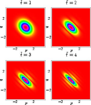
Figure 2.3: $|F^{(2)}(p,\uparrow;q,\downarrow;t)_{t}|$ versus $p$, $q$ at $\tilde{t}=1,2,3,4$.

We have applied the method for obtaining the Schmidt decomposition given in Ref. [LL05a] (see Chapter 8, or a more complete description in Ref. [Lam05]) to Eq. (2.2), considering for the orthonormal functions $\{O^{(1)}(p)\}$, $\{O^{(2)}(q)\}$ Hermite polynomials with their weights, to take advantage of the two Gaussian functions. We obtain the Schmidt decomposition for $\tilde{t}=1,2,3,4$, where the error with matrices $C_{mn}$ $12\times 12$ or smaller is $d^{2}_{m_{0},n_{0}}\leq 7\cdot 10^{-3}$ in all considered cases. We plot in Fig. 2.4 the coefficients $\lambda_{n}$ of the Schmidt decomposition of Eq. (2.2) as a function of $n$, for times $\tilde{t}=1,2,3,4$. The number of $\lambda_{n}$ different from zero increases as time is elapsed, and thus the entanglement grows.

The complete Schmidt decomposition, including channels $t$ and $u$, is given in terms of Slater determinants [SCK⁺01], and is usually called Slater decomposition. It is obtained antisymmetrizing the amplitude for channel $t$

$$F^{(2)}(p,s_{1};q,s_{2};t)\propto\sum_{n}\sqrt{\lambda_{n}(\tilde{t})}\frac{\psi^{(1)}_{n}(p,\tilde{t})|\!\!\uparrow\rangle\psi^{(2)}_{n}(q,\tilde{t})|\!\!\downarrow\rangle-\psi^{(2)}_{n}(p,\tilde{t})|\!\!\downarrow\rangle\psi^{(1)}_{n}(q,\tilde{t})|\!\!\uparrow\rangle}{\sqrt{2}},$$

(2.29)

where the modes $\psi^{(1)}_{n}(k,\tilde{t})$ and $\psi^{(2)}_{n}(k,\tilde{t})$ are the Schmidt modes of the channel $t$ obtained for particles $1$ and $2$ respectively, and they correspond to the modes of the channel $u$ for particles $2$ and $1$ respectively.

Figure 2.4: Eigenvalues $\lambda_{n}$ versus $n$ at times $\tilde{t}=1,2,3,4$.

A measure of the entanglement of a pure bipartite state of the form of Eq. (2.29), equivalent to the entropy of entanglement $S$, is given by the Slater number [GRE94]

$$K:=\frac{1}{\sum_{n=0}^{\infty}\lambda_{n}^{2}}\,.$$ (2.30)

$K$ gives the number of effective Slater determinants which appear in a certain pure bipartite state in the form of Eq. (2.29). The larger the value of $K$, the larger the entanglement. For $K=1$ (one Slater determinant) there is no entanglement. This measure is obtained considering the average probability, which is given by $\sum_{n=0}^{\infty}\lambda_{n}^{2}$ ($\sum_{n=0}^{\infty}\lambda_{n}=1$, and thus $\{\lambda_{n}\}$ can be seen as a probability distribution). The inverse of the average probability is the Slater number. Its attractive properties are that it is independent of the representation of the wavefunction, it is gauge invariant, and it reaches its minimum value of 1 for the separable state (single Slater determinant). In Fig. 2.5, we show the Slater number $K$ as a function of elapsed time $\tilde{t}$, verifying that the entanglement increases as the system evolves. It can be appreciated in this figure the monotonic growth of entanglement, due to the fact that we have considered an incident electron with well defined momentum. In realistic physical situations with wave packets, this growth would stop, due to the momentum spread of the initial electrons. The general trend is that the higher the precision in the incident electron momentum, the larger the resulting asymptotic entanglement. The fact that the entanglement in momenta between the two fermions increases with time is a consequence of the interaction between them. We remark that the entanglement cannot grow unless the two particles “feel” each other. The correlations in momenta are not specific of QED: the effect of any interaction producing momentum exchange while conserving total momentum will translate into momentum correlations.

Figure 2.5: Slater number $K$ as a function of the elapsed time $\tilde{t}$.

The Schmidt modes in momenta space for the amplitude of Eq. (2.2) are given by

$$\psi^{(\alpha)}_{m}(k,\tilde{t}) \simeq \mathrm{e}^{-k^{2}/2}\sum_{n=0}^{n_{0}}(\sqrt{\pi}2^{n}n!)^{-1/2}A^{(\alpha)}_{mn}(\tilde{t})H_{n}(k)\;\;\;\;$$

$$\alpha = 1,2,$$ (2.31)

where $n_{0}$ is the corresponding cut-off and the values of the coefficients $A^{(\alpha)}_{mn}(\tilde{t})$ are obtained through the method given in Ref. [LL05a]. The modes in momenta space depend on time because they are not stationary states: the QED dynamics between the two fermions and the indeterminacy on the energy at early stages of the interaction give this dependence. By construction, the coefficients $A^{(\alpha)}_{mn}(\tilde{t})$ do not depend on $p$, $q$.

We plot in Fig. 2.6 the Schmidt modes $\psi^{(1)}_{n}(p,\tilde{t})$ at times $\tilde{t}=1,2,3,4$ for $n=0,1,2,3$ (we are plotting specifically the real part of each mode only, which approximates well the whole mode, because Eq. (2.2) is almost real for the cases considered). The sharper modes for each $n$ correspond to the later times. Each Schmidt mode is well approximated at early times by the corresponding Hermite orthonormal function, and afterwards it sharpens and deviates from that function: it gets corrections from higher order polynomials. The fact that the modes get thinner with time is related to the behavior of Eq. (2.2) at large times. In particular the sinc function goes to $\delta(p+q)$ and thus the amplitude gets sharper.

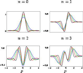
Figure 2.6: Schmidt modes $\psi^{(1)}_{n}(p,\tilde{t})$ at times $\tilde{t}=1,2,3,4$ for $n=0,1,2,3$. The sharper modes for each $n$ correspond to the later times.

Now we consider the Schmidt modes in configuration space. To obtain them, we just Fourier transform the modes of Eq. (2.31) with respect to the momenta $p_{1}$, $p_{2}$

$$\tilde{\psi}^{(\alpha)}_{m}(x_{\alpha},\tilde{t})=\frac{1}{\sqrt{2\pi}}\int_{-\infty}^{\infty}dp_{\alpha}\mathrm{e}^{i(p_{\alpha}x_{\alpha}-\frac{p_{\alpha}^{2}}{2m}t)}\psi^{(\alpha)}_{m}(k(p_{\alpha}),\tilde{t}),$$ (2.32)

where $\alpha=1,2$. The dependence of $p$ on $p_{1}$ and $q$ on $p_{2}$ is given through Eq. (2.22). The factor $\mathrm{e}^{-i\frac{p_{\alpha}^{2}}{2m}t}$ in Eq. (2.32) is the one which commutes the states between the interaction picture (considered in Eq. (2.31) and in the previous calculations in Secs. 2.1 and 2.2) and the Schrödinger picture.

The Hermite polynomials obey the following expression [GR48]

$$\int_{-\infty}^{\infty}dx\mathrm{e}^{-(x-y)^{2}}H_{n}(\alpha x)=\sqrt{\pi}(1-\alpha^{2})^{n/2}H_{n}\left(\frac{\alpha y}{\sqrt{1-\alpha^{2}}}\right).$$ (2.33)

With the help of Eq. (2.33) and by linearity of the Fourier transforms, we are able to obtain analytic expressions for the Schmidt modes in configuration space (to a certain accuracy, which depends on the cut-offs considered). This is possible because the dispersion relation of the massive fermions in the considered non-relativistic limit is $E_{\alpha}=\frac{p_{\alpha}^{2}}{2m}$, and thus the integral of Eq. (2.32) can be obtained analytically using Eq. (2.33).

The corresponding Schmidt modes in configuration space are then given by

$$\tilde{\psi}^{(\alpha)}_{m}(\tilde{x}_{\alpha},\tilde{t})\simeq\sum_{n=0}^{n_{0}}A^{(\alpha)}_{mn}(\tilde{t})\tilde{O}^{(\alpha)}_{n}(\tilde{x}_{\alpha},\tilde{t}),\;\;\;\;\alpha=1,2,$$ (2.34)

where the orthonormal functions in configuration space are

$$\tilde{O}^{(\alpha)}_{n}(\tilde{x}_{\alpha},\tilde{t})=i^{n}(\sqrt{\pi}2^{n}n!)^{-1/2}\frac{\mathrm{e}^{-in\arctan(\tilde{\sigma}\tilde{t})+i\tilde{\sigma}^{-1}(\tilde{x}_{\alpha}-\tilde{t}/2)}}{\sqrt{1+i\tilde{\sigma}\tilde{t}}}\mathrm{e}^{-\frac{(\tilde{x}_{\alpha}-\tilde{t})^{2}}{2(1+i\tilde{\sigma}\tilde{t})}}H_{n}\left[\frac{\tilde{t}-\tilde{x}_{\alpha}}{\sqrt{1+(\tilde{\sigma}\tilde{t})^{2}}}\right].$$ (2.35)

In Eqs. (2.34) and (2.35), we are using dimensionless variables, $\tilde{x}_{\alpha}=\frac{\sigma x_{\alpha}}{\sqrt{2}}$, $\alpha=1,2$, $\tilde{\sigma}=\frac{\sigma}{p_{a}^{0}}$, and the dimensionless time defined before, $\tilde{t}=\frac{p_{a}^{0}\sigma}{2m}t$. The modes in Eqs. (2.34) and (2.35) are normalized in the variables $\tilde{x}_{\alpha}$. The orthonormal functions of Eq. (2.35) propagate in space at a speed $\frac{p_{a}^{0}}{\sqrt{2}m}$ and they spread in their evolution. Additionally, the modes of Eq. (2.34) have also the time dependence of $A^{(\alpha)}_{mn}(\tilde{t})$. The Slater decomposition in configuration space, obtained Fourier transforming the modes of Eq. (2.31) is

$$\tilde{F}^{(2)}(\tilde{x}_{1},\tilde{x}_{2},\tilde{t})\propto\sum_{n}\sqrt{\frac{\lambda_{n}(\tilde{t})}{2}}[\tilde{\psi}^{(1)}_{n}(\tilde{x}_{1},\tilde{t})|\!\!\uparrow\rangle\tilde{\psi}^{(2)}_{n}(\tilde{x}_{2},\tilde{t})|\!\!\downarrow\rangle-\tilde{\psi}^{(2)}_{n}(\tilde{x}_{1},\tilde{t})|\!\!\downarrow\rangle\tilde{\psi}^{(1)}_{n}(\tilde{x}_{2},\tilde{t})|\!\!\uparrow\rangle].$$

(2.36)

The coefficients $\lambda_{n}(\tilde{t})$ are unaffected by the Fourier transformation, and thus the degree of entanglement in configuration space is the same as in momenta space.

We consider now the initial spin configuration

$$|s_{a}^{0}s_{b}^{0}\rangle=|\!\!\uparrow\uparrow\rangle,$$ (2.37)

where, the only possible final state in the non-relativistic limit is

$$|s_{1}s_{2}\rangle=|\!\!\uparrow\uparrow\rangle.$$ (2.38)

In this case, the sinc term goes to zero, because the momentum part of this term is antisymmetric in $p^{2}$, $q^{2}$ and the sinc function goes to $\delta(p+q)$, which has support (as a distribution) on $q=-p$. We point out that the sinc contribution to this amplitude is negligible because of the particular setup chosen. In other experiment configurations the amplitude in Eq. (2.19) associated to the spin states of Eqs. (2.37) and (2.38) would have appreciable sinc term and thus increasing momenta entanglement with time. On the other hand, in this case the contribution from $\Upsilon_{t}(t)$ in Eq. (2.1) and $\Upsilon_{u}(t)$ is even smaller than the sinc term, and converges weakly to zero.

We plot in Fig. 2.7 the real and imaginary parts of the term associated to $\Upsilon_{t}(t)$ and $\Upsilon_{u}(t)$ in Eq. (2.23), which we denote by $g(p,q,\tilde{t})$, for spin states of Eqs. (2.37) and (2.38) as a function of time $\tilde{t}\in(1,1.001)$ and having $p=1$, $q=1.2$. We want to show with it the strong oscillatory character of the amplitude with time, and how all the contributions interfere destructively with each other giving a zero final value. This is similar to the stationary phase procedure, in which only the contributions in proximity to the stationary value of the phase do interfere constructively and are appreciable. What we display here is the weak convergence to zero for the functions $\Upsilon_{t}(t)$ and $\Upsilon_{u}(t)$.

Figure 2.7: Real and imaginary parts of the amplitude $g(p,q,\tilde{t})$ for $p=1$, $q=1.2$, and $\tilde{t}\in(1,1.001)$ (arbitrary units).

In this section, we investigated the generation of entanglement in momenta between two identical spin-$\frac{1}{2}$ particles which interact via QED. We showed how the correlations grow as the energy conservation is increasingly fulfilled with time. The previous calculation had, however, the approximation of considering a projectile particle with perfectly well defined momentum, something not achievable in practice. This is a first step towards a real experiment, where both fermions will have a dispersion in momenta and thus infinite entanglement will never be reached, due to the additional integrals of the Dirac delta $\delta(\Delta E)$ over the momentum spread. We believe these results have much interest both from the fundamental point of view but also from the experimental one, for example in fermion gases [SALW04].

2.3 Entanglement transfer between momentum and spin

2.3.1 Dynamical transfer and distillation

In the previous section we computed the entanglement in momenta for a pair of electrons which interact through exchange of a virtual photon. The results could be summarized by: the more collimated in momentum is the incident electron, and the more time is elapsed, the larger the entanglement in momenta obtained. Heisenberg’s principle, on the other hand, establishes a limit to the precision with which the momentum may be collimated and hence to the achievable degree of entanglement.

It is possible in principle to transform the entanglement in momenta into entanglement in spins. This is easily seen in terms of the majorization criterion [Nie99, NC00]. This is of practical interest because the experimenter usually manipulates spins, thus spin entanglement seems to be more useful. Here we analyze this entanglement transfer.

Majorization is an area of mathematics which predates quantum mechanics. Quoting Nielsen and Chuang, “Majorization is an ordering on d-dimensional real vectors intended to capture the notion that one vector is more or less disordered than another”. We consider a pair of $d$-dimensional vectors, $x=(x_{1},...,x_{d})$ and $y=(y_{1},...,y_{d})$. We say $x$ is majorized by $y$, written $x\prec y$, if $\sum_{j=1}^{k}x_{j}^{\downarrow}\leq\sum_{j=1}^{k}y_{j}^{\downarrow}$ for $k=1,...,d$, with equality instead of inequality for $k=d$. We denote by $z^{\downarrow}$ the components of $z$ in decreasing order $(z_{1}^{\downarrow}\geq z_{2}^{\downarrow}\geq...\geq z_{d}^{\downarrow})$. The interest of this work in the majorization concept comes from a theorem which states that a bipartite pure state $|\psi\rangle$ may be transformed to another pure state $|\phi\rangle$ by Local Operations and Classical Communication (LOCC) if and only if $\lambda_{\psi}\prec\lambda_{\phi}$, where $\lambda_{\psi}$, $\lambda_{\phi}$ are the vectors of (square) coefficients of the Schmidt decomposition (A.11) (finite dimension case) or (A.14) (continuous case) of the states $|\psi\rangle$, $|\phi\rangle$, respectively. LOCC adds to those quantum operations effected only locally the possibility of classical communication between spatially separated parts of the system. According to this criterion, it would be possible in principle to obtain a singlet spin state $|\phi\rangle$ beginning with a momentum entangled state $|\psi\rangle$ whenever $\lambda_{\psi}\prec\lambda_{\phi}$.

The possibility of obtaining a singlet spin state from a momentum-entangled state can be extended to a more efficient situation: the possibility of distillation of entanglement. This idea consists on obtaining multiple singlet states beginning with several copies of a given pure state $|\psi\rangle$. The distillable entanglement of $|\psi\rangle$ consists in the ratio $n/m$, where $m$ is the number of copies of $|\psi\rangle$ we have initially, and $n$ the number of singlet states we are able to obtain via LOCC acting on these copies. It can be shown [NC00] that for pure states the distillable entanglement equals the entropy of entanglement, S (11.2). Thus, in the continuous case (infinite-dimensional Hilbert space), the distillable entanglement is not bounded from above, because neither is S. According to this, the larger the entanglement in momenta the more singlet states could be obtained with LOCC.

To illustrate the possibility of entanglement transfer with a specific example, we consider a momentum-entangled state for two distinguishable fermions

$$|\psi\rangle=\frac{1}{\sqrt{2}}[\psi^{(1)}_{1}(p)\psi^{(2)}_{1}(q)+\psi^{(1)}_{2}(p)\psi^{(2)}_{2}(q)]\otimes|\!\!\uparrow\uparrow\rangle.$$ (2.39)

This state has associated a vector $\lambda_{\psi}^{\downarrow}=(1/2,1/2,0,0,...)$. On the other hand, the singlet state

$$|\phi\rangle=\psi^{(1)}_{1}(p)\psi^{(2)}_{1}(q)\otimes\frac{1}{\sqrt{2}}(|\!\!\uparrow\downarrow\rangle-|\!\!\downarrow\uparrow\rangle)$$ (2.40)

has associated a vector $\lambda_{\phi}^{\downarrow}=(1/2,1/2,0,0...)$.

These vectors obey $\lambda_{\psi}\prec\lambda_{\phi}$, and thus the state entangled in momenta may be transformed into the state entangled in spins via LOCC. The operations needed to achieve this are in general unitary operations acting on the degrees of freedom of momentum and spin of each individual electron, local projective measurements, and classical communication between the separated parts of the system (the experimental setups located where the electrons reach). The unitary local operations may be implemented by, for example (in the non-relativistic case), electric fields (which modify the momentum) and magnetic fields (which modify the spin and the direction of the momentum) combined to give the desired effect. The specific setup needed to do this might be rather complicated. In addition, decoherence effects should be avoided. What we point out is that majorization states this transformation would be possible in principle.

2.3.2 Kinematical transfer and Lorentz boosts

Another approach to the study of entanglement transfer between momentum and spin degrees of freedom is the kinematical one. In fact, the Lorentz transformations may entangle the spin and momentum degrees of freedom. To be more explicit, and following the notation of Ref. [GA02], we consider a certain bipartite pure wave function $g_{\lambda\sigma}(\mathbf{p},\mathbf{q})$ for two spin-$\frac{1}{2}$ fermions, where $\lambda$ and $\sigma$ denote respectively the spin degrees of freedom of each of the two fermions, and $\mathbf{p}$ and $\mathbf{q}$ the corresponding momenta. This would appear to an observer in a Lorentz transformed frame as

$$g_{\lambda\sigma}(\mathbf{p},\mathbf{q})\begin{array}[]{c}\Lambda\\ \longrightarrow\end{array}\sum_{\lambda^{\prime}\sigma^{\prime}}U_{\lambda\lambda^{\prime}}^{(\Lambda^{-1}\mathbf{p})}U_{\sigma\sigma^{\prime}}^{(\Lambda^{-1}\mathbf{q})}g_{\lambda^{\prime}\sigma^{\prime}}(\Lambda^{-1}\mathbf{p},\Lambda^{-1}\mathbf{q}),$$ (2.41)

where

$$U_{\lambda\lambda^{\prime}}^{(\mathbf{p})}:=D_{\lambda\lambda^{\prime}}^{(1/2)}(R(\Lambda,\mathbf{p}))$$ (2.42)

is the spin $\frac{1}{2}$ representation of the Wigner rotation $R(\Lambda,\mathbf{p})$. The Wigner rotations of Eq. (2.42) can be seen as conditional logical operators, which rotate the spin a certain angle depending on the value of the momentum. Thus, a Lorentz transformation will modify in general the entanglement between momentum and spin of each individual electron. We distinguish the following particular cases.

Product state in all variables. In this case,

$$g_{\lambda\sigma}(\mathbf{p},\mathbf{q})=g_{1}(\mathbf{p})g_{2}(\mathbf{q})|\lambda\rangle|\sigma\rangle,$$ (2.43)

and the entanglement at the rest reference frame is zero. Under a boost, the Wigner rotations of Eq. (2.42) entangle the momentum of each fermion with its spin, and thus the entanglement momentum-spin grows [PST02].

Entangled state spin-spin and/or momentum-momentum. We consider now a state

$$g_{\lambda\sigma}(\mathbf{p},\mathbf{q})=f(\mathbf{p},\mathbf{q})|\phi\rangle$$ (2.44)

with $|\phi\rangle$ an arbitrary state of the spins, and $f(\mathbf{p},\mathbf{q})$ an arbitrary state of the momenta. In this case, a Lorentz boost will entangle in general each spin with its corresponding momentum, and a careful analysis shows that the spin-spin entanglement never grows [GA02]. Of course, by applying the reversed boost the entanglement momentum-spin would be transferred back to the spin-spin one, and thus the latter would grow. This particular case shows that, for the state we considered in Sec. 2.2, given by Eqs. (2.24), (2.25) and (2.2), the entanglement could not be transferred from momenta into spins via Lorentz transformations. Thus, the dynamical approach would be here more suitable.

Entangled state momentum-spin. According to the previous theorem, the momentum-spin entanglement may be lowered, transferring part of the correlations to the spins, or increased, taking some part of the correlations from them. To my knowledge, there is not a similar result for the momentum, that is, whether the momentum entanglement can be preserved under boosts, or it suffers decoherence similarly to the spins, and part of it is transferred to the momentum-spin part.

Chapter 3 Generation of spin entanglement via spin-independent scattering

3.1 Spin-spin entanglement via spin-independent scattering

A compound system is entangled when it is impossible to attribute a complete set of properties to any of its parts. In this case, and for pure states, it is impossible to factor the state in a product of independent factors belonging to its parts. In this chapter we will consider bipartite systems composed of two $s=\textstyle\frac{1}{2}$ fermions. Our aim is to uncover [LL06] some specific features that apply when both particles are identical. They appear itemized three pages below.

States of two identical fermions have to obey the symmetrization postulate. This implies that they decompose into linear combinations of Slater determinants (SLs) of individual states. Naively, as these SLs cannot be factorized further, indistinguishability seems to imply entanglement. This is reinforced by the observation that the entropy of entanglement (EoE) is bounded from below by $S\geq 1$, well above the lower limit $S=0$ for a pair of non-entangled distinguishable particles. So, it looks like there is an inescapable amount of uncertainty, and hence of entanglement, in any state of two identical fermions.

The above issue has been extensively examined in the literature [SCK⁺01, ESBL02, GM04] with the following result: Part of the uncertainty (giving $S=1$) corresponds to the impossibility to individuate which one is the first or the second particle of the system. This explains why the lower limit for the EoE is 1. Consider for instance two identical $s=\textstyle\frac{1}{2}$ fermions in a singlet state

$$\chi_{S}:=\frac{1}{\sqrt{2}}[\chi(1)^{\uparrow}\chi(2)^{\downarrow}-\chi(1)^{\downarrow}\chi(2)^{\uparrow}].$$

The antisymmetrization does not preclude the assignment of properties to the particles, but only assigning them precisely to particle 1 or particle 2. The reduced density matrix of any of the particles is $\rho=\frac{1}{2}I$ with an EoE $S(\rho)=1$.

The portion of $S$ above 1 (if any) is genuine entanglement as it corresponds to the impossibility of attributing precise properties to the particles of the system [GM04]. Assume for instance that we endow the previous fermions with the capability of being outside ($\chi=\psi$) or inside ($\chi=\varphi$) the laboratory ($(\psi^{i},\psi^{j})=\delta^{ij}$, $(\varphi^{i},\varphi^{j})=\delta^{ij}$, $(\psi^{i},\varphi^{j})=0$, $i,j=\uparrow,\downarrow$). We now have two different possibilities: either the fermion outside has spin up ($\psi^{\uparrow}$) or spin down ($\psi^{\downarrow}$). Hence, there are two different SLs for a system built by a pair of particles with opposite spins, one outside, the other inside the laboratory

$${\rm SL}(1,2)_{1} = \frac{1}{\sqrt{2}}[\psi(1)^{\uparrow}\,\varphi(2)^{\downarrow}-\varphi(1)^{\downarrow}\,\psi(2)^{\uparrow}],$$

$${\rm SL}(1,2)_{2} = \frac{1}{\sqrt{2}}[\psi(1)^{\downarrow}\,\varphi(2)^{\uparrow}-\varphi(1)^{\uparrow}\,\psi(2)^{\downarrow}].$$ (3.1)

They form two different biorthogonal states, the combination $[{\rm SL}(1,2)_{1}-{\rm SL}(1,2)_{2}]/\sqrt{2}$ corresponding to the singlet and $[{\rm SL}(1,2)_{1}+{\rm SL}(1,2)_{2}]/\sqrt{2}$ to the triplet state (with respect to the total spin $\mathbf{s}=\mathbf{s}_{1}+\mathbf{s}_{2}$). An arbitrary state $\Phi(1,2)$ would then be a linear combination of these two SLs:

$$\Phi(1,2)\,=\,c_{1}{\rm SL}(1,2)_{1}\,+\,c_{2}{\rm SL}(1,2)_{2},\,\,\sum_{i}|c_{i}|^{2}=1,$$ (3.2)

giving an EoE

$$S\,=\,1-\sum_{i}|c_{i}|^{2}\,\log_{2}|c_{i}|^{2}\,\geq\,1.$$ (3.3)

Clearly, when $c_{1}$ or $c_{2}$ vanish, we come back to $S=1$, as the only uncertainty left is the very identity of the particles. Summarizing, while indistinguishability is an issue to be solved by antisymmetrization within each SL, entanglement is an issue pertaining to the superposition of different SLs [SCK⁺01, ESBL02, GM04]. At the end, we could even decide to call 1 to the variables of the outside particle, and forget about symmetrization

$$\Phi(1,2)\rightarrow\,c_{1}\psi(1)^{\uparrow}\,\varphi(2)^{\downarrow}\,+\,c_{2}\psi(1)^{\downarrow}\,\varphi(2)^{\uparrow},$$ (3.4)

as both particles are far away from each other. In this case, the EoE, equal to $S=\,-\sum_{i}|c_{i}|^{2}\,\log_{2}|c_{i}|^{2}\geq 0$ is lesser than the one corresponding to antisymmetrized states by a quantity of 1, which is just the uncertainty associated to antisymmetrization. From now on we will consider the latter definition of $S$, which gives the genuine amount of entanglement between the two particles. Notice that for half-odd $s$, the number $\#{\rm{\rm SL}}$ of Slater determinants is bounded by $\#{\rm{\rm SL}}\leq(2s+1)d/2$, where $d$ is the dimension of each Hilbert space of the configuration or momentum degrees of freedom for each of the two fermions.

Much in the same way as above, we could consider one of the particles as right moving ($\chi=\psi_{0}$) the other as left moving ($\chi=\psi_{\pi}$), giving rise to two SLs in parallel with the above discussion. This is the first step towards the inclusion of the full set of commuting operators for the system. In addition to the spin components ($s_{1},s_{2}$) or helicities, there are the total $\mathbf{P}$ and relative $\mathbf{p}$ momenta. In the center of mass (CoM) frame we could consider the system described by the continuum of SLs

$${\rm SL}(1,2;\mathbf{p})_{s} = \frac{1}{\sqrt{2}}[\psi(1)_{0}^{s}\,\psi(2)_{\pi}^{-s}-\psi(1)_{\pi}^{-s}\,\psi(2)_{0}^{s}],$$

$${\rm SL}(1,2;\mathbf{p})_{-s} = \frac{1}{\sqrt{2}}[\psi(1)_{0}^{-s}\,\psi(2)_{\pi}^{s}-\psi(1)_{\pi}^{s}\,\psi(2)_{0}^{-s}],$$ (3.5)

where $\psi(1)_{0}^{s}=\langle 1|\mathbf{p}\,s\rangle$ and $\psi(1)_{\pi}^{s}=\langle 1|-\mathbf{p}\,s\rangle$. The labels 0 and $\pi$ are the azimuthal angles when we laid the axes along $\mathbf{p}$. Finally, there is a pair of SLs for each $\mathbf{p}$, so that a general state made with two opposite spin particles with relative momentum $\mathbf{p}$ could be written in the form:

$$\Phi(1,2)_{\mathbf{p}}^{0}\,=\,\sum_{s=\pm 1/2}\,c_{s}(\mathbf{p})\,{\rm SL}(1,2;\mathbf{p})_{s},$$ (3.6)

with $\sum_{s=\pm 1/2}\,|c_{s}(\mathbf{p})|^{2}=1$. Again, we run into the impossibility to tell which is 1 and which is 2. In addition there may be some uncertainty about the total spin state, whether a singlet or a triplet, or conversely, about the spin component of any of the particles, $\psi_{0}$ or $\psi_{\pi}$.

After this discussion it should be clear to what extent entanglement and distinguishability belong to different realms [SCK⁺01, ESBL02, GM04]. A requirement to include identical particles is to symmetrize the expressions used for unlike particles. Until now, we have only considered the free case. We have to examine the case of two interacting particles, as interaction is expected to be the source of subsequent entanglement [LRM76, Tör85, ALP01, PS03, MY04, AAMS04, SALW04, Har05, TK05, LLS06b, Wan05, Har06b, Har06a, HW06]. Obviously, the answer may depend on a tricky way on the detailed form of the interaction, of its spin dependence in particular . It also seems that the role of particles identity, if any, will be played through symmetrization.

In the following we will show that spin entanglement is generated for the case of two interacting spin-$\textstyle\frac{1}{2}$ identical particles, with the following features:

• Spin-spin entanglement is generated even by spin independent interactions.

• In this case, it is independent of any symmetrization procedure.

• This phenomenon does not appear for unlike particles.

We first tackle the scattering of two unequal $s=\textstyle\frac{1}{2}$ particles $A$ and $B$ which run into each other with relative CoM momentum $\mathbf{p}$. We set the frame axes by the initial momentum $\mathbf{p}$ of particle $A$, and let the spin components be $s_{a}=s$ and $s_{b}=-s$ along an arbitrary but fixed axis. We will consider a spin independent Hamiltonian $H$, so the evolution conserves $\mathbf{s}_{a}$ and $\mathbf{s}_{b}$. We denote by $A_{\theta}^{s}$ $(B_{\theta}^{s})$ the state of particle $A$ ($B$) that propagates along direction $\theta$ with spin $s$. In these conditions the scattering proceeds as:

$$\Phi_{\mbox{in}}=\,A_{0}^{s}\,B_{\pi}^{-s}\longrightarrow\,\Phi_{\mbox{out}}(\theta)=\,f_{p}(\theta)\,A_{\theta}^{s}\,B_{\pi-\theta}^{-s},$$ (3.7)

where $\theta$ is the scattering angle and $f_{p}(\theta)$ the scattering amplitude. We will consider $\theta$ different from 0 or $\pi$ to avoid forward and backward directions. While the increase of uncertainty due to the interaction is clear, because a continuous manifold of final directions with probabilities $|f_{p}(\theta)|^{2}$ opened up from just one initial direction, spin remains untouched. The information about $s_{a}$ is the same before and after the scattering; as much as we knew the initial spin of $A$, we know its final spin whatever the final direction is. In other words, spin was not entangled by the interaction. We will now translate these well known facts to the case of identical particles, where they do not hold true.

Let particle $B$ be identical to $A$. Consider the same initial state as before: A particle $A$ with momentum $\mathbf{p}$ and spin $s$ runs into another $A$ with momentum $-\mathbf{p}$ and spin $-s$. Notice there is maximal information on the state. We could write $\Phi_{\mbox{in}}=\,A_{0}^{s}A_{\pi}^{-s}$, and eventually symmetrize. We now focus on the final state. It is no longer true that particle $A$ will come out with momentum $\mathbf{p^{\prime}}$ and spin $s$ with amplitude $f_{p}(\theta)$ while the amplitude for coming out with momentum $\mathbf{p^{\prime}}$ and spin $-s$ vanishes. Recalling that $B$ above did become $A$, the two cases $f_{p}(\theta)A_{\theta}^{s}B_{\pi-\theta}^{-s}$ and $f_{p}(\pi-\theta)A_{\pi-\theta}^{s}B_{\theta}^{-s}$ fuse into a unique state

$$\Phi_{\mbox{out}}(\theta)=f_{p}(\theta)\,A_{\theta}^{s}\,A_{\pi-\theta}^{-s}+f_{p}(\pi-\theta)\,A_{\pi-\theta}^{s}\,A_{\theta}^{-s},$$ (3.8)

as shown in Figure 3.1.

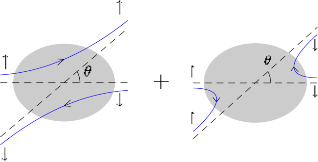
Figure 3.1: Schematic picture of the two channels that contribute to the spin-independent scattering of two identical fermions. The shaded regions denote an arbitrary spin-independent interaction between the two fermions. The vertical arrows $\uparrow$, $\downarrow$ indicate the corresponding third component of spin.

Notice the uncertainty acquired by the spin: Now particle $A$ comes out from the interaction along $\theta$ either with spin $s$ or with spin $-s$, with relative amplitudes $f_{p}(\theta)$ and $f_{p}(\pi-\theta)$ respectively. In other words, spin was entangled during the spin independent evolution. Here, it is not the spin dependence of the interaction, but the existence of additional degrees of freedom which generate spin-spin entanglement. These, act as ancillas creating an effective spin-spin interaction that entangles the two fermions. The ancilla and the degree of entanglement depend on the scattering angle $\theta$. Notice that for $\theta=\pi/2$ both amplitudes $f_{p}(\theta)$ and $f_{p}(\pi-\theta)$ become equal, so that the degree of generated entanglement is maximal, 1 ebit. On the other hand, for $\theta\simeq 0$, it generally holds $f_{p}(\theta)\gg f_{p}(\pi-\theta)$, so that in the forward and backward scattering almost no entanglement would be generated. However, this depends on the specific interaction. In Section 3.2 we will clarify this point with Coulomb interaction.

Symmetrization does not change this, it only expresses that we can not tell which one is 1 and which one is 2. The properly symmetrized initial state is

$$\Phi_{\mbox{in}}={\rm SL}(1,2;\mathbf{p})_{s}=\frac{1}{\sqrt{2}}[A(1)_{0}^{s}A(2)_{\pi}^{-s}-A(1)_{\pi}^{-s}A(2)_{0}^{s}].$$ (3.9)

The scattering process could be written in terms of SLs as

$${\rm SL}(1,2;\mathbf{p})_{s}\longrightarrow f_{p}(\theta)\,{\rm SL}(1,2;\mathbf{p}^{\prime})_{s}-f_{p}(\pi-\theta)\,{\rm SL}(1,2;\mathbf{p}^{\prime})_{-s},$$ (3.10)

where $\mathbf{p}^{\prime}$ is the final momentum and the Slater determinants are given in (3.5). Both, this expression and Eq.(3.8), describe the same physical situation and lead to the same entanglement generation.

The bosonic case may be analyzed in an analogous way. The modification for two-dimensional spin Hilbert spaces (i.e. photons) would be a sign change in Eqs. (3.5), (3.9) and (3.10), as bosonic statistics has associated symmetric states. The equivalent of Eq. (3.10) for bosons is a genuine entangled state for $\theta\neq 0,\pi$, much as in the fermionic case.

3.2 A specific example: Coulomb interaction at lowest order

We now consider Coulomb interaction at lowest order to illustrate the reasonings presented above. In this case

$$f_{p}(\theta) = \frac{N(e)}{t(\theta)},$$

$$f_{p}(\pi-\theta) = \frac{N(e)}{u(\theta)},$$ (3.11)

where $N(e)$ is a numerical factor depending on the charge $e$. $t(\theta)$ and $u(\theta)$ are two of the Mandelstam variables, associated to $t$ and $u$ channels respectively, and depending on the scattering angle $\theta$. for initial $p$ and final $p^{\prime}$ relative 4-momenta of the scattering fermions, they are given by $t=(p-p^{\prime})^{2}$, $u=(p+p^{\prime})^{2}$. In the CoM frame,

$$t(\theta)\!\! := 2(m^{2}-E^{2})(1-\cos\theta),$$

$$u(\theta)\!\! := 2(m^{2}-E^{2})(1+\cos\theta),$$ (3.12)

where $m$ is the mass of each fermion and $2E$ is the available energy.

According to this, the spin part of the state (3.8) for this case, properly normalized, is

$$|\chi_{\theta}\rangle=f_{+}(\theta)|\!\!\uparrow\downarrow\rangle-f_{-}(\theta)|\!\!\downarrow\uparrow\rangle,$$ (3.13)

being

$$f_{\pm}(\theta):=\frac{1\pm\cos\theta}{\sqrt{2(1+\cos^{2}\theta)}}.$$ (3.14)

The two amplitudes $f_{+}$ and $f_{-}$ vary monotonously as $\theta$ grows, becoming equal for $\theta=\pi/2$. The physical meaning for this is that for $\theta\rightarrow 0$, the knowledge about the system is maximal and the entanglement minimal (zero), and for increasing $\theta$ the knowledge of the system decreases continuously until reaching its minimum value at $\theta=\pi/2$. Accordingly, the entanglement grows with $\theta$ until reaching its maximum value for $\theta=\pi/2$.

We plot in Figure 3.2 the EoE [TK05] $S(\theta)=-f_{+}(\theta)^{2}\log_{2}f_{+}(\theta)^{2}-f_{-}(\theta)^{2}\log_{2}f_{-}(\theta)^{2}$ of state (3.13) as a function of $\theta$, for $0<\theta\leq\pi/2$. The entanglement grows monotonically until $\theta=\pi/2$, where it becomes maximal (1 ebit).

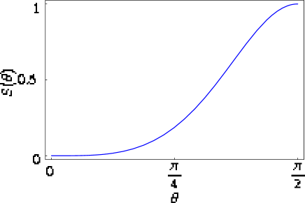
Figure 3.2: EoE $S(\theta)$ as a function of $\theta$.

3.3 Violation of Bell’s inequality as a function of the scattering angle $\theta$

In order to analyze the role the $\theta$ scattering angle plays in the generation of these genuine quantum correlations, we consider now the degree of violation of Bell’s inequality as a function of $\theta$. To this purpose, we define [Bel64, CS78] the observable

$$E(\mathbf{\hat{a}},\mathbf{\hat{b}}) := \langle\Phi|(\mathbf{\sigma}^{(1)}\cdot\mathbf{\hat{a}}\otimes\mathbf{\sigma}^{(2)}\cdot\mathbf{\hat{b}})|\Phi\rangle$$

$$= -[\hat{a}_{z}\hat{b}_{z}+2f_{p}(\theta)f_{p}(\pi-\theta)(\hat{a}_{x}\hat{b}_{x}+\hat{a}_{y}\hat{b}_{y})],$$

where $|\Phi\rangle:=|\Phi_{\rm out}(\theta)\rangle$ is the (normalized) state (3.8) and $\mathbf{\hat{a}}$, $\mathbf{\hat{b}}$ are arbitrary unit vectors. In Eq. (3.3) we consider the amplitudes $f_{p}(\theta)$ and $f_{p}(\pi-\theta)$ normalized for each $\theta$, in the form $|f_{p}(\theta)|^{2}+|f_{p}(\pi-\theta)|^{2}=1$. We consider three coplanar unit vectors, $\mathbf{\hat{a}}$, $\mathbf{\hat{b}}$ and $\mathbf{\hat{c}}$. $(\widehat{\mathbf{\hat{a}},\mathbf{\hat{b}}})=\pi/3$, $(\widehat{\mathbf{\hat{a}},\mathbf{\hat{c}}})=2\pi/3$ and $(\widehat{\mathbf{\hat{b}},\mathbf{\hat{c}}})=\pi/3$. We have

$$|E(\mathbf{\hat{a}},\mathbf{\hat{b}})-E(\mathbf{\hat{a}},\mathbf{\hat{c}})|=1,$$

$$F(\theta):=1+E(\mathbf{\hat{b}},\mathbf{\hat{c}})=\frac{5}{4}-\frac{3}{2}f_{p}(\theta)f_{p}(\pi-\theta).$$ (3.16)

The Bell’s inequality, given by [Bel64, CS78]

$$|E(\mathbf{\hat{a}},\mathbf{\hat{b}})-E(\mathbf{\hat{a}},\mathbf{\hat{c}})|\leq 1+E(\mathbf{\hat{b}},\mathbf{\hat{c}}),$$ (3.17)

will then be

$$F(\theta)\geq 1.$$ (3.18)

For the particular case of Coulomb interaction at lowest order here considered, $2f_{p}(\theta)f_{p}(\pi-\theta)=2f_{+}(\theta)f_{-}(\theta)=(1-\cos^{2}\theta)/(1+\cos^{2}\theta)$ and thus the critical angle for which the inequality becomes violated is $\theta_{c}=\pi/4$ for $F(\theta_{c})=1$. For $\theta_{c}<\theta\leq\pi/2$ the Bell’s inequality does not hold. We show in Figure 3.3 the $\theta$ dependence of $F(\theta)$ together with the classical-quantum border, $F=1$, at $\theta_{c}=\pi/4$. Thus, for experiments with $\theta>\pi/4$ one could be able in principle to discriminate between local realism and quantum mechanics.

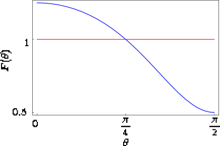
Figure 3.3: $F(\theta)$ as a function of $\theta$. The classical-quantum border corresponds to $F(\theta_{c})=1$, with $\theta_{c}=\pi/4$.

This is in contrast with recent analysis of Bell’s inequality violation in elementary particle systems [Go04, BEG05, Tör86], where the emphasis was placed on flavor entanglement, $K^{0}\bar{K}^{0}$, $B^{0}\bar{B}^{0}$, and the like. These analysis presented [BBGH04] two kinds of drawbacks coming from the lack of experimenter’s free will and from the unitary evolution with decaying states. These issues reduce the significance of the experiments up to the point of preventing their use as tests of quantum mechanics versus local realistic theories. The spin-spin entanglement analyzed in this chapter does not have this kind of problems and could be used in principle for that purpose.

3.4 The tripartite case

Our protocol can be straightforwardly generalized to more complicated settings. To show this, we consider now three identical, massive, $s=1$ particles which interact through some kind of two- and three-body interaction, which for our practical purposes is completely general, but spin independent. We suppose the particles evolve in a plane, and the prolongations of the directions of propagation intersect at one point, having relative angles of $2\pi/3$ degrees among each two neighbor directions, see Figure 3.4. We will label these in-directions with angles 0, $2\pi/3$ and $4\pi/3$, which will also be the final angles for illustrative purposes. Our initial state is now

$$\Phi_{\mbox{in}}=\,A_{0}^{0}A_{2\pi/3}^{1}A_{4\pi/3}^{-1},$$ (3.19)

where $A_{\theta}^{s}$ denotes, like previously, the state of particle of type $A$ with propagation direction $\theta$ and spin $s$. Our final state will now be a superposition of all the possible final states associated to the different channels. There are as much as permutations of the three states $A^{0}$, $A^{1}$ and $A^{-1}$, which can evolve each through directions $0$, $2\pi/3$ and $4\pi/3$.

For example, in case there is no interaction, the three states will evolve according to $A_{0}^{0}\rightarrow A_{0}^{0}$, $A_{2\pi/3}^{1}\rightarrow A_{2\pi/3}^{1}$, and $A_{4\pi/3}^{-1}\rightarrow A_{4\pi/3}^{-1}$. We will give a weight $f_{0,0,0}$ to this channel, where the 0 labels mean the in- and out-angle for each particle remains the same.

In the case where there is a two-body interaction among the particles, the possible channels are those which permutate two of the final legs of the Feynman diagram. There are three channels associated to two-body scattering: $\{0\rightarrow 2\pi/3,2\pi/3\rightarrow 0,4\pi/3\rightarrow 4\pi/3\}$, $\{0\rightarrow 4\pi/3,2\pi/3\rightarrow 2\pi/3,4\pi/3\rightarrow 0\}$, and $\{0\rightarrow 0,2\pi/3\rightarrow 4\pi/3,4\pi/3\rightarrow 2\pi/3\}$. One example would be the following evolution, $A_{0}^{0}\rightarrow A_{2\pi/3}^{0}$, $A_{2\pi/3}^{1}\rightarrow A_{0}^{1}$, and $A_{4\pi/3}^{-1}\rightarrow A_{4\pi/3}^{-1}$. As in previous sections, the spins remain unchanged. We will give a weight $f_{2\pi/3,2\pi/3,0}$ to the channels associated to two-body interactions, which means that two of the particles experience a trajectory change of $2\pi/3$.

Finally, in case there is a three-body interaction among the three particles, the final channels will be those that permutate the three legs of the Feynman diagram. The two available channels for three-body interactions are $\{0\rightarrow 2\pi/3,2\pi/3\rightarrow 4\pi/3,4\pi/3\rightarrow 0\}$ and $\{0\rightarrow 4\pi/3,2\pi/3\rightarrow 0,4\pi/3\rightarrow 2\pi/3\}$. One example would be the evolution $A_{0}^{0}\rightarrow A_{2\pi/3}^{0}$, $A_{2\pi/3}^{1}\rightarrow A_{4\pi/3}^{1}$, and $A_{4\pi/3}^{-1}\rightarrow A_{0}^{-1}$. We will give a weight $f_{2\pi/3,2\pi/3,2\pi/3}$ to the channels associated to three-body scattering, which means that the three particles change their propagation direction by $2\pi/3$. Of course, three-body interactions are unusual, so typically we will have $f_{0,0,0}\gg f_{2\pi/3,2\pi/3,0}\gg f_{2\pi/3,2\pi/3,2\pi/3}$. Accordingly, the final state obtained this way will be

$$\Phi_{\mbox{out}} = f_{0,0,0}A_{0}^{0}A_{2\pi/3}^{1}A_{4\pi/3}^{-1}$$ (3.20)

$$+f_{2\pi/3,2\pi/3,0}[A_{2\pi/3}^{0}A_{0}^{1}A_{4\pi/3}^{-1}+A_{4\pi/3}^{0}A_{2\pi/3}^{1}A_{0}^{-1}+A_{0}^{0}A_{4\pi/3}^{1}A_{2\pi/3}^{-1}]$$

$$+f_{2\pi/3,2\pi/3,2\pi/3}[A_{2\pi/3}^{0}A_{4\pi/3}^{1}A_{0}^{-1}+A_{4\pi/3}^{0}A_{0}^{1}A_{2\pi/3}^{-1}].$$

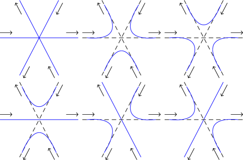
Figure 3.4: Schematic diagrams for the tripartite spin-independent scattering of three identical $s=1$ particles. The spins associated to the incident directions are $s=0$ ($\theta_{\rm in}=0$), $s=1$ ($\theta_{\rm in}=2\pi/3$), and $s=-1$ ($\theta_{\rm in}=4\pi/3$) in all the six cases.

We plot in Figure 3.4 the six different diagrams associated to the six channels of the spin-independent scattering of three identical $s=1$ particles.

In the asymptotic limit, once the particles are far apart, their wave packets will not overlap anymore and we may consider the particles as distinguishable. We will denote by $|s_{1},s_{2},s_{3}\rangle$ the spin state of the three particles, where $s_{1}$ is associated to the particle that propagates at the end along $0$, $s_{2}$ to the one that propagates along $2\pi/3$ and $s_{3}$ to the one that moves along $4\pi/3$. The asymptotic spin state associated to Eq. (3.20) will be, in this notation,

$$|\chi\rangle = f_{0,0,0}|0,1,-1\rangle$$ (3.21)

$$+f_{2\pi/3,2\pi/3,0}[|1,0,-1\rangle+|-1,1,0\rangle+|0,-1,1\rangle]$$

$$+f_{2\pi/3,2\pi/3,2\pi/3}[|1,-1,0\rangle+|-1,0,1\rangle].$$

Notice that in case we considered only two spins, $1=0$ and $-1$ (either three spin-$\frac{1}{2}$ particles or three spin-1 particles with just two spin states of the 3-dimensional $s=1$ Hilbert space), the part associated to two-body interaction would be a $W$ state, a state with genuine tripartite entanglement. Thus, in this way it could be possible to generate genuine multipartite entanglement via spin-independent scattering. A generalization to the $N$-partite case of our procedure is straightforward from the tripartite and bipartite cases and we will omit it here.

In summary, we analyzed the relation between entanglement and antisymmetrization for identical particles, in the context of spin-independent particle scattering. We showed that, in order to create genuine spin-spin quantum correlations between two $s=\textstyle\frac{1}{2}$ fermions, spin-dependent interactions are not compulsory. The identity of the particles along with an interaction between degrees of freedom different from the spin, suffice for this purpose. The entanglement generated this way is not a fictitious one due to antisymmetrization, but a real one, and violates a certain Bell’s inequality for $\theta>\theta_{c}=\pi/4$.

Chapter 4 Relativity of distillability

4.1 Lorentz transformed spin density matrix

As we have pointed out along this Thesis, nowadays entanglement is considered a basic resource in present and future applications of quantum information, communication, and technology [NC00, GMD02]. However, entangled states are fragile, and interactions with the environment destroy their coherence, thus degrading this precious resource. Fortunately, entanglement can still be recovered from a certain class of states which share the property of being distillable. This means that even in a decoherence scenario, entanglement can be extracted through purification processes that restore their quantum correlations [BBP⁺96, BMD05]. An entangled state can be defined as a quantum state that is not separable, and a separable state can always be expressed as a convex sum of product density operators [Wer89]. In particular, a bipartite separable state can be written as $\rho=\sum_{i}C_{i}\rho^{(\rm a)}_{i}\otimes\rho^{(\rm b)}_{i}$, where $C_{i}\geq 0$, $\sum_{i}C_{i}=1$, and $\rho^{(\rm a)}_{i}$ and $\rho^{(\rm b)}_{i}$ are density operators associated to subsystems A and B.

In the context of quantum field theory, special relativity (SR) [Rin01] and quantum mechanics are described in a unified manner. From a fundamental point of view, in addition, it is relevant to study the implications of SR on the modern quantum information theory (QIT) [PT04]. Recently, Peres et al. [PST02] have observed that the entropy of entanglement of a single spin-$\frac{1}{2}$ density matrix is not a relativistic invariant, given that Wigner rotations [Wig39] entangle the spin with its momentum distribution when observed in a moving referential. This astonishing result, intrinsic and unavoidable, shows that entanglement theory must be reconsidered from a relativistic point of view. On the other hand, the fundamental implications of relativity on quantum mechanics could be stronger than what is commonly believed. For example, Wigner rotations induce also decoherence on two entangled spins [AM02, PS03, GA02, GBA03]. However, they have not been studied yet in the context of mixed states and distillable entanglement [Per96, HHH98].

A typical situation in SR pertains to a couple of observers: one is stationary in an inertial frame $\cal{S}$ and the other is also stationary in an inertial frame $\cal{S}^{\prime}$ that moves with velocity $\mathbf{v}$ with respect to $\cal{S}$. The problems addressed in SR consider the relation between different measurements of physical properties, like velocities, time intervals, and space intervals, of objects as seen by observers in $\cal{S}$ and $\cal{S}^{\prime}$. However, in QIT, it is assumed that the measurements always take place in a proper reference frame, either $\cal{S}$ or $\cal{S}^{\prime}$. To see the effects that SR can bring about in QIT problems [PT04], we need to enlarge the typical situations where quantum descriptions and measurements take place.

In order to analyze the new possibilities that SR offers, we introduce [LMDS06] the following concepts

• Weak isoentangled state $\rho^{\rm WIE}$: A state that is entangled in all considered reference frames. This property is independent of the chosen entanglement measure ${\cal E}$.

• Strong isoentangled state $\rho^{\rm SIE}_{\cal E}$: A state that is entangled in all considered reference frames, while having a constant value associated with a given entanglement measure ${\cal E}$. This concept depends on the ${\cal E}$ chosen.

• Weak isodistillable state $\rho^{\rm WID}$: A state that is distillable in all considered reference frames. This implies that the state is entangled for these observers.

• Strong isodistillable state $\rho^{\rm SID}_{\cal E}$: A state that is distillable in all considered reference frames, while having a constant value associated with a given entanglement measure ${\cal E}$. This concept depends on the ${\cal E}$ chosen.

In general, the following hierarchy of sets holds (see Fig. 4.1 for a pictorial representation)

$$\{\rho^{\rm WIE}\}\supset\{\rho^{\rm SIE}_{\cal E}\}\supset\{\rho^{\rm SID}_{\cal E}\}\subset\{\rho^{\rm WID}\}\subset\{\rho^{\rm WIE}\}.$$ (4.1)

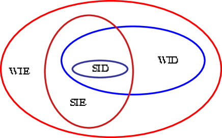
Figure 4.1: Hierarchy for the sets of states WIE, SIE, WID, and SID.

To illustrate the relative character of distillability, let us consider [LMDS06] the specific situation in which Alice (A) and Bob (B) share a bipartite mixed state of Werner type with respect to an inertial frame $\cal{S}$. Moreover, in order to complete the SR+QIT scenario, we also consider another inertial frame $\cal{S}^{\prime}$, where relatives (A’) and (B’) of Alice (A) and Bob (B) are moving with relative velocity $\mathbf{v}$ with respect to $\cal{S}$. Using the picture of Einstein’s trains, we may think that (A) and (B) are at the platform of the railway station sharing a set of mixed states, while their relatives (A’) and (B’) are travelling in a train sharing another couple of entangled particles of the same characteristics. The mixed state is made up of two particles, say electrons with mass $m$, having two types of degrees of freedom: momentum $\mathbf{p}$ and spin $s=\frac{1}{2}$. The former is a continuous variable while the latter is a discrete one. By definition, we consider our logical or computational qubit to be the spin degree of freedom. Each particle is assumed to be localized, like in a box, and its momentum $\mathbf{p}$ will be described by the same Gaussian distribution. We assume that the spin degrees of freedom of particles $A$ and $B$ are decoupled from their respective momentum distributions and form the state

$$\rho^{AB}_{\cal{S}}:=F|\Psi^{-}_{\mathbf{p}}\rangle\langle\Psi^{-}_{\mathbf{p}}|+\frac{1-F}{3}\bigg{(}|\Psi^{+}_{\mathbf{p}}\rangle\langle\Psi^{+}_{\mathbf{p}}|+|\Phi^{-}_{\mathbf{p}}\rangle\langle\Phi^{-}_{\mathbf{p}}|+|\Phi^{+}_{\mathbf{p}}\rangle\langle\Phi^{+}_{\mathbf{p}}|\bigg{)}.$$ (4.2)

Here, $F$ is a parameter such that $0\leq F\leq 1$,

$$|\Psi^{-}_{\mathbf{p}}\rangle\!\!\! := \!\!\!\frac{1}{\sqrt{2}}[\Psi_{1}^{(\rm a)}(\mathbf{p_{a}})\Psi_{2}^{(\rm b)}(\mathbf{p_{b}})-\Psi_{2}^{(\rm a)}(\mathbf{p_{a}})\Psi_{1}^{(\rm b)}(\mathbf{p_{b}})]$$

$$|\Psi^{+}_{\mathbf{p}}\rangle\!\!\! := \!\!\!\frac{1}{\sqrt{2}}[\Psi_{1}^{(\rm a)}(\mathbf{p_{a}})\Psi_{2}^{(\rm b)}(\mathbf{p_{b}})+\Psi_{2}^{(\rm a)}(\mathbf{p_{a}})\Psi_{1}^{(\rm b)}(\mathbf{p_{b}})]$$

$$|\Phi^{-}_{\mathbf{p}}\rangle\!\!\! := \!\!\!\frac{1}{\sqrt{2}}[\Psi_{1}^{(\rm a)}(\mathbf{p_{a}})\Psi_{1}^{(\rm b)}(\mathbf{p_{b}})-\Psi_{2}^{(\rm a)}(\mathbf{p_{a}})\Psi_{2}^{(\rm b)}(\mathbf{p_{b}})]$$

$$|\Phi^{+}_{\mathbf{p}}\rangle\!\!\! := \!\!\!\frac{1}{\sqrt{2}}[\Psi_{1}^{(\rm a)}(\mathbf{p_{a}})\Psi_{1}^{(\rm b)}(\mathbf{p_{b}})+\Psi_{2}^{(\rm a)}(\mathbf{p_{a}})\Psi_{2}^{(\rm b)}(\mathbf{p_{b}})],\,\,\,\,\,$$ (4.3)

where $\mathbf{p_{a}}$ and $\mathbf{p_{b}}$ are the corresponding momentum vectors of particles $A$ and $B$, as seen in $\cal{S}$, and

$$\Psi_{1}^{(\rm a)}(\mathbf{p_{a}}) := {\cal G}(\mathbf{p_{a}})|\!\!\uparrow\rangle=\left(\begin{array}[]{cccc}{\cal G}(\mathbf{p_{a}})\\ 0\\ \end{array}\right)$$ (4.6)

$$\Psi_{2}^{(\rm a)}(\mathbf{p_{a}}) := {\cal G}(\mathbf{p_{a}})|\!\!\downarrow\rangle=\left(\begin{array}[]{cccc}0\\ {\cal G}(\mathbf{p_{a}})\\ \end{array}\right)$$ (4.9)

$$\Psi_{1}^{(\rm b)}(\mathbf{p_{b}}) := {\cal G}(\mathbf{p_{b}})|\!\!\uparrow\rangle=\left(\begin{array}[]{cccc}{\cal G}(\mathbf{p_{b}})\\ 0\\ \end{array}\right)$$ (4.12)

$$\Psi_{2}^{(\rm b)}(\mathbf{p_{b}}) := {\cal G}(\mathbf{p_{b}})|\!\!\downarrow\rangle=\left(\begin{array}[]{cccc}0\\ {\cal G}(\mathbf{p_{b}})\\ \end{array}\right),$$ (4.15)

with Gaussian momentum distribution ${\cal G}(\mathbf{p}):=\pi^{-3/4}w^{-3/2}\exp(-{\rm p}^{2}/2w^{2})$, being ${\rm p}:=|\mathbf{p}|$. $|\!\!\uparrow\rangle$ and $|\!\!\downarrow\rangle$ represent spin vectors pointing up and down along the $z$-axis, respectively. If we trace momentum degrees of freedom in Eq. (4.3), we obtain the usual spin Bell states, $\{|\Psi^{-}\rangle,|\Psi^{+}\rangle,|\Phi^{-}\rangle,|\Phi^{+}\rangle\}$. If we do the same in Eq. (4.2), we remain with the usual spin Werner state [Wer89] that can be written in its matrix form as

$$\left(\begin{array}[]{cccc}\frac{1-F}{3}&0&0&0\\ 0&\frac{2F+1}{6}&\frac{1-4F}{6}&0\\ 0&\frac{1-4F}{6}&\frac{2F+1}{6}&0\\ 0&0&0&\frac{1-F}{3}\\ \end{array}\right).$$ (4.16)

It is known that Bell state $|\Psi^{-}\rangle$ is distillable out of Eq. (4.16) if, and only if, $F>1/2$.

We consider also another pair of similar particles, $A^{\prime}$ and $B^{\prime}$, with the same state as $A$ and $B$, $\rho^{A^{\prime}B^{\prime}}_{\cal{S}^{\prime}}=\rho^{AB}_{\cal{S}}$, but seen in another reference frame $\cal{S}^{\prime}$. The frame $\cal{S}^{\prime}$ moves with velocity $\mathbf{v}$ along the $x$-axis with respect to the frame $\cal{S}$.

When we want to describe the state of $A^{\prime}$ and $B^{\prime}$ as observed from frame $\cal{S}$, rotations on the spin variables, conditioned to the value of the momentum of each particle, have to be introduced. These conditional spin rotations, considered first by Wigner [Wig39], are a natural consequence of Lorentz transformations. In general, Wigner rotations entangle spin and momentum degrees of freedom for each particle. We want to encode quantum information in the two qubits determined by the spin degrees of freedom of our two spin-$\frac{1}{2}$ particles. As a consequence, the reduced spin system, after a Lorentz transformation, increases its entropy and reduces its initial degree of entanglement. If we consider the velocities of the particles as having only non-zero components in the $z$-axis, each state vector of $A^{\prime}$ and $B^{\prime}$ in Eq. (4.15) transforms as

$$\Psi_{1}(\mathbf{p})=\left(\begin{array}[]{cccc}{\cal G}(\mathbf{p})\\ 0\\ \end{array}\right)\rightarrow\Lambda[\Psi_{1}(\mathbf{p})]=\left(\begin{array}[]{cccc}\cos\theta_{\mathbf{p}}\\ \sin\theta_{\mathbf{p}}\\ \end{array}\right){\cal G}(\mathbf{p})$$ (4.21)

$$\Psi_{2}(\mathbf{p})=\left(\begin{array}[]{cccc}0\\ {\cal G}(\mathbf{p})\\ \end{array}\right)\rightarrow\Lambda[\Psi_{2}(\mathbf{p})]=\left(\begin{array}[]{cccc}-\sin\theta_{\mathbf{p}}\\ \,\,\,\,\,\cos\theta_{\mathbf{p}}\\ \end{array}\right){\cal G}(\mathbf{p}),$$ (4.26)

(4.27)

where $\cos\theta_{\mathbf{p}}$ and $\sin\theta_{\mathbf{p}}$ express Wigner rotations conditioned to the value of the momentum vector.

The most general bipartite density matrix in the rest frame for arbitrary spin-$\frac{1}{2}$ states and Gaussian product states in momentum, is spanned by the tensor products of $\Psi^{(\rm a)}_{1}$, $\Psi^{(\rm a)}_{2}$, $\Psi^{(\rm b)}_{1}$, and $\Psi^{(\rm b)}_{2}$, and can be expressed as

$$\rho=\sum_{ijkl=1,2}C_{ijkl}\Psi^{(\rm a)}_{i}(\mathbf{p_{a}})\otimes\Psi^{(\rm b)}_{j}(\mathbf{p_{b}})[\Psi^{(\rm a)}_{k}(\mathbf{p_{a}^{\prime}})\otimes\Psi^{(\rm b)}_{l}(\mathbf{p_{b}^{\prime}})]^{{\dagger}}.$$ (4.28)

Under a boost, Eq. (4.28) will transform into

$$\Lambda\rho\Lambda^{{\dagger}}=\sum_{ijkl=1,2}C_{ijkl}\Lambda^{(a)}[\Psi^{(a)}_{i}(\mathbf{p_{a}})]\otimes\Lambda^{(b)}[\Psi^{(b)}_{j}(\mathbf{p_{b}})]\{\Lambda^{(a)}[\Psi^{(a)}_{k}(\mathbf{p_{a}^{\prime}})]\otimes\Lambda^{(b)}[\Psi^{(b)}_{l}(\mathbf{p_{b}^{\prime}})]\}^{{\dagger}}.$$

(4.29)

Tracing out the momentum degrees of freedom, we obtain

$$\mathrm{Tr}_{\rm\mathbf{p_{a}},\mathbf{p_{b}}}(\Lambda\rho\Lambda^{{\dagger}}) = \sum_{ijkl=1,2}C_{ijkl}\mathrm{Tr}_{\rm\mathbf{p_{a}}}(\Lambda^{(\rm a)}[\Psi^{(\rm a)}_{i}(\mathbf{p_{a}})]\{\Lambda^{(\rm a)}[\Psi^{(\rm a)}_{k}(\mathbf{p_{a}})]\}^{{\dagger}})$$ (4.30)

$$\otimes\mathrm{Tr}_{\rm\mathbf{p_{b}}}(\Lambda^{(\rm b)}[\Psi^{(\rm b)}_{j}(\mathbf{p_{b}})]\{\Lambda^{(\rm b)}[\Psi^{(\rm b)}_{l}(\mathbf{p_{b}})]\}^{{\dagger}}).$$

Following Peres et al. [PST02], we compute first the Lorentz transformed density matrix of state $\Psi_{1}$, after tracing out the momentum. The expression is given, to leading order of $w/m\ll 1$, by

$$\mathrm{Tr}_{\rm\mathbf{p}}[\Lambda\Psi_{1}(\Lambda\Psi_{1})^{{\dagger}}]=\frac{1}{2}\left(\begin{array}[]{cc}1+n_{z}^{\prime}&0\\ 0&1-n_{z}^{\prime}\end{array}\right),$$ (4.31)

where

$$n^{\prime}_{z}:=1-\left(\frac{w}{2m}\tanh\frac{\alpha}{2}\right)^{2},$$ (4.32)

and $\cosh\alpha:=\gamma=(1-\beta^{2})^{-1/2}$. Demanding $w/m$ to be small does not restrict the generality of our results, on the contrary, it is a requirement of physical consistency in our model. First, the Newton-Wigner localization problem prevents us from considering momentum distributions with $w\sim m$. In that case, particle creation would manifest and our model, relying on a bipartite state of the Fock space, would break down. Second, $w\sim m$ would produce a very fast wave-packet spreading, having as a consequence an undesired particle delocalization. Finally, thinner packets favor the possibility of finding isoentangled and isodistillable states.

This can be straightforwardly generalized to the other three tensor products involving $\Psi_{1}$ and $\Psi_{2}$,

$$\mathrm{Tr}_{\rm\mathbf{p}}[\Lambda\Psi_{2}(\Lambda\Psi_{2})^{{\dagger}}] = \frac{1}{2}\left(\begin{array}[]{cc}1-n_{z}^{\prime}&0\\ 0&1+n_{z}^{\prime}\end{array}\right),$$ (4.35)

$$\mathrm{Tr}_{\rm\mathbf{p}}[\Lambda\Psi_{1}(\Lambda\Psi_{2})^{{\dagger}}] = \frac{1}{2}\left(\begin{array}[]{cc}0&1+n^{\prime}_{z}\\ -(1-n_{z}^{\prime})&0\end{array}\right),$$ (4.38)

$$\mathrm{Tr}_{\rm\mathbf{p}}[\Lambda\Psi_{2}(\Lambda\Psi_{1})^{{\dagger}}] = \frac{1}{2}\left(\begin{array}[]{cc}0&-(1-n^{\prime}_{z})\\ 1+n_{z}^{\prime}&0\end{array}\right).$$ (4.41)

With the help of Eqs. (4.30-4.41), it is possible to compute the effects of the Lorentz transformation on any density matrix of two spin-$\frac{1}{2}$ particles, after tracing out the momentum, for a boost in the $x$-direction.

4.2 Application to Werner states

With these tools, we compute now the Lorentz transformation, under a boost, of the state in Eq. (4.2) and obtain the reduced spin state

$$\left(\!\!\!\begin{array}[]{cccc}\frac{1}{4}+c_{F}{n^{\prime}_{z}}^{2}&0&0&c_{F}({n^{\prime}_{z}}^{2}-1)\\ 0&\frac{1}{4}-c_{F}{n^{\prime}_{z}}^{2}&c_{F}({n^{\prime}_{z}}^{2}+1)&0\\ 0&c_{F}({n^{\prime}_{z}}^{2}+1)&\frac{1}{4}-c_{F}{n^{\prime}_{z}}^{2}&0\\ c_{F}({n^{\prime}_{z}}^{2}-1)&0&0&\frac{1}{4}+c_{F}{n^{\prime}_{z}}^{2}\\ \end{array}\!\!\!\right),\\$$ (4.42)

where $c_{F}:=\frac{1-4F}{12}$. We can apply now the positive partial transpose (PPT) criterion [Per96, HHH96] to know whether this state is entangled. Due to the box-inside-box structure of Eq. (4.42), it is possible to diagonalize its partial transpose in a simple manner, finding the following eigenvalues

$$x_{1}=\frac{2F+1}{6}$$

$$x_{2}=\frac{1-F}{3}+\frac{1-4F}{6}{n^{\prime}_{z}}^{2}$$

$$x_{3}=\frac{1-F}{3}-\frac{1-4F}{6}{n^{\prime}_{z}}^{2}$$

$$x_{4}=\frac{2F+1}{6}.$$ (4.43)

Given that $F>0$, $x_{1}$ and $x_{4}$ are always positive, and $x_{3}$ can be shown to be positive for $0<{n^{\prime}_{z}}<1$. The eigenvalue $x_{2}$ is negative if, and only if, $F>N^{\prime}_{z}$, where $N^{\prime}_{z}:=(2+{n^{\prime}_{z}}^{2})/(2+4{n^{\prime}_{z}}^{2})$. The latter implies that in the interval

$$\frac{1}{2}<F<N^{\prime}_{z}$$ (4.44)

distillability of state $|\Psi^{-}\rangle$ is possible for the spin state in A and B, but impossible for the spin state in A’ and B’, both described in frame $\cal{S}$. We plot in Fig. 4.2 the behavior of $N^{\prime}_{z}$ as a function of the rapidity $\alpha$. The region below the curve (ND) corresponds to the $F$ values for which distillation is not possible in the Lorentz transformed frame. On the other hand, the region above the curve (D), corresponds to states which are distillable for the corresponding values of $n^{\prime}_{z}$. Notice that there are values of $F$ for which the Werner states are weak isodistillable and weak isoentangled, corresponding to the states in the region D above the curve for the considered range of $n^{\prime}_{z}$. On the other hand, there are states that will change from distillable (entangled) into separable for a certain value of $n^{\prime}_{z}$, showing the relativity of distillability and separability.

Figure 4.2: $N^{\prime}_{z}$ of Eq. (4.44) as function of the rapidity $\alpha$, for $w/2m=0.1$.

4.3 Analysis of existence of SIE and SID states

The study of strongly isoentangled and strongly isodistillable two-spin states is a much harder task that will depend on the entanglement measure we choose. We believe that these cases impose demanding conditions and, probably, this kind of states does not exist. However we would like to give a plausibility argument to justify this conjecture. Our argument is based on two mathematical points: (i) analytic continuation is a mathematical tool that allows to extend the analytic behavior of a function to a region where it was not initially defined, and (ii) an analytic function is either constant or it changes along all its interval of definition. Point (i) will allow us to extend analytically our calculation to $n^{\prime}_{z}=0$, an unphysical but mathematically convenient limit. Point (ii) will be applied to any well-behaved entanglement measure. We consider then a general spin density matrix

$$\rho:=\left(\!\!\!\begin{array}[]{cccc}a_{1}&b_{1}&b_{2}&b_{3}\\ b_{1}^{*}&a_{2}&c_{1}&c_{2}\\ b_{2}^{*}&c_{1}^{*}&a_{3}&d\\ b_{3}^{*}&c_{2}^{*}&d^{*}&a_{4}\\ \end{array}\!\!\!\right),$$ (4.49)

where $a_{1}$, $a_{2}$, $a_{3}$, and $a_{4}$ are real, and $\sum_{i}a_{i}=1$. The analytic continuation of the Lorentz transformed state, according to our procedure in Eqs. (4.30-4.41), in the limit $n^{\prime}_{z}\rightarrow 0$, is

$$\left(\!\!\!\begin{array}[]{cccc}1/4&\frac{i(\mathrm{\Im}b_{1}+\mathrm{\Im}d)}{2}&\frac{i(\mathrm{\Im}b_{2}+\mathrm{\Im}c_{2})}{2}&\frac{(\mathrm{\Re}b_{3}-\mathrm{\Re}c_{1})}{2}\\ \frac{-i(\mathrm{\Im}b_{1}+\mathrm{\Im}d)}{2}&1/4&\frac{(-\mathrm{\Re}b_{3}+\mathrm{\Re}c_{1})}{2}&\frac{i(\mathrm{\Im}b_{2}+\mathrm{\Im}c_{2})}{2}\\ \frac{-i(\mathrm{\Im}b_{2}+\mathrm{\Im}c_{2})}{2}&\frac{(-\mathrm{\Re}b_{3}+\mathrm{\Re}c_{1})}{2}&1/4&\frac{i(\mathrm{\Im}b_{1}+\mathrm{\Im}d)}{2}\\ \frac{(\mathrm{\Re}b_{3}-\mathrm{\Re}c_{1})}{2}&\frac{-i(\mathrm{\Im}b_{2}+\mathrm{\Im}c_{2})}{2}&\frac{-i(\mathrm{\Im}b_{1}+\mathrm{\Im}d)}{2}&1/4\\ \end{array}\!\!\!\right),$$ (4.53)

(4.54)

where $\Re$ and $\Im$ denote the real and imaginary parts. This state is separable because its eigenvalues, given by

$$\lambda_{1} = \frac{1}{4}[1-2\mathrm{\Re}(b_{3}-c_{1})+2\mathrm{\Im}(b_{1}+b_{2}+c_{2}+d)]$$

$$\lambda_{2} = \frac{1}{4}[1-2\mathrm{\Re}(b_{3}-c_{1})-2\mathrm{\Im}(b_{1}+b_{2}+c_{2}+d)]$$

$$\lambda_{3} = \frac{1}{4}[1+2\mathrm{\Re}(b_{3}-c_{1})+2\mathrm{\Im}(b_{1}-b_{2}-c_{2}+d)]$$

$$\lambda_{4} = \frac{1}{4}[1+2\mathrm{\Re}(b_{3}-c_{1})-2\mathrm{\Im}(b_{1}-b_{2}-c_{2}+d)],\,\,\,\,\,\,$$ (4.55)

coincide with the corresponding ones for the partial transpose matrix. In this case, $\lambda_{1}\leftrightarrow\lambda_{4}$, and $\lambda_{2}\leftrightarrow\lambda_{3}$. So, according to the PPT criterion, the analytic continuation of the Lorentz transformed density matrix of all the two spin-$\frac{1}{2}$ particle states with Gaussian momentum part factorizable considered here, converges to a separable state in the limit of $n^{\prime}_{z}\rightarrow 0$. Our analytic calculation holds for $n^{\prime}_{z}\lesssim 1$, leaving out of reach the case $n^{\prime}_{z}=0$. However, any analytic measure of entanglement, due to this behavior of the analytic continuation at $n^{\prime}_{z}=0$, is forced to change with $n^{\prime}_{z}$ for $n^{\prime}_{z}\lesssim 1$, except for states separable in all frames. In this way, our approximation techniques give evidence of the non-existence of strong isoentangled and strong isodistillable states, for variations of the parameter $n^{\prime}_{z}$.

From a broader perspective, our analysis corresponds to the invariance of entanglement and distillability of a two spin-$\frac{1}{2}$ system under Lorentz-Wigner completely positive (CP) maps [HHH96]. This is an important problem that, to our knowledge, has not received much attention in quantum information theory, and that will require a separate and more abstract analysis. Moreover, for higher dimensional spaces, like a two spin-$1$ system (qutrits), the notion of relativity of bound entanglement will also arise [HHH98].

In summary, the concepts of weak and strong isoentantangled and isodistillable states were introduced, which should help to understand the relationship between special relativity and quantum information theory. The study of Werner states allowed us to show that distillability is a relative concept depending on the frame in which it is considered. We have proven the existence of weak isoentangled and weak isodistillable states in our range of validity of the parameter $n^{\prime}_{z}$. We also conjectured the non-existence of strong isoentangled and strong isodistillable states in special relativity. We give evidence for this surprising result relying on the analytic continuation of the Lorentz transformed spin density matrix for a general two spin-$\frac{1}{2}$ particle state. This analytic continuation converges to a separable state in the limit $n^{\prime}_{z}\rightarrow 0$. Thus, any entanglement measure analytic in the parameter $n^{\prime}_{z}$ is forced to change with $n^{\prime}_{z}$ in every interval, unless the state is separable in every frame.

Chapter 5 Dirac equation and relativistic effects in a single trapped ion

5.1 Dirac equation simulation in a trapped ion

The search for a fully relativistic Schrödinger equation gave rise to the Klein-Gordon and Dirac equations [Sak67]. P. A. M. Dirac looked for a Lorentz-covariant wave equation that is linear in spatial and time derivatives, expecting that the interpretation of the square wave function as a probability density holds. As a result, he obtained a fully covariant wave equation for a spin-$1/2$ massive particle (fermion), which incorporated ab initio the spin degree of freedom. It is known that the Dirac formalism plays a central role in the context of quantum field theory, where creation and annihilation of particles are allowed. However, the one-particle solutions of the Dirac equation in relativistic quantum mechanics predict some astonishing effects, like Zitterbewegung, Klein’s paradox, Wigner rotations, and mass acquisition through spontaneous symmetry breaking produced by a Higgs boson.

In recent years, a growing interest has appeared regarding simulations of relativistic effects in controllable physical systems. Some examples are the simulation of Unruh effect in trapped ions [ADM05], Zitterbewegung for massless fermions in solid state physics [SLW05], and the simulation of black-hole properties in the realm of Bose-Einstein condensates [GACZ00]. In this respect, simulation of the paradigmatic Dirac equation in a completely flexible and controllable physical system would be desirable, given its many counterintuitive and unverified predictions. This problem arises mainly due to the fact that the required range of energies (or frequencies) is of the order of the fermion mass $m$, unaccessible to present experiments.

On the other hand, the fresh dialog between quantum information and special relativity [PST02, AM02, PS03, PT04] has raised important issues concerning the content and transfer of quantum information under Lorentz transformations. In this sense, the so-called Wigner rotations entangle the spin with the momentum degrees of freedom, yielding a non-covariant spin entropy for a single particle and reducing the degree of entanglement in multiparticle systems [LMDS06].

In this chapter, I study the simulation of the Dirac equation in a single trapped ion. We show [LLSS07b] that it is possible to implement realistic interactions on four metastable ionic internal levels, coupled to the motional degrees of freedom, so as to reproduce such a fundamental quantum relativistic wave equation. In this manner, the Dirac dynamics could be fully simulated and many relevant quantum relativistic effects reproduced and measured.

We consider a single ion inside a Paul trap, where four metastable ionic internal states, $|a\rangle,|b\rangle,|c\rangle$, and $|d\rangle$, may be coupled pairwise to the center-of-mass (CM) motional degrees of freedom in directions $x$, $y$, and $z$. We will make use of three standard interactions in trapped ion technology, allowing for the coherent control of the vibronic dynamics [LBMW03]. First, a carrier interaction consisting of a coherent driving acting on any pair of internal levels, while leaving untouched the motional degrees of freedom. It can be described by the Hamiltonian $H_{\sigma_{x}}=\hbar\Omega_{x}(\sigma^{+}+\sigma^{-})=\hbar\Omega_{x}\sigma_{x}$, where $\sigma^{+}$ and $\sigma^{-}$ are the raising and lowering spin-$1/2$ operators, respectively, and $\Omega_{x}$ is the coupling strength. The driving phases and frequencies could be adjusted so as to produce, alternatively, the Hamiltonians $H_{\sigma_{y}}=\hbar\Omega_{y}\sigma_{y}$ and $H_{\sigma_{z}}=\hbar\Omega_{z}\sigma_{z}$, where $\sigma_{x}$, $\sigma_{y}$, and $\sigma_{z}$, are Pauli operators in the conventional directions $x$, $y$, and $z$. Second, a Jaynes-Cummings (JC) interaction, usually called red-sideband excitation, consisting of a coherent driving acting on two internal levels and one of the CM modes. Typically, a resonant JC coupling induces an excitation in the internal levels while producing a deexcitation of the motional harmonic oscillator, and viceversa. The JC Hamiltonian reads $H_{\rm JC}=\hbar g(\sigma^{+}a+\sigma^{-}a^{\dagger})$, where $a$ and $a^{\dagger}$ are the annihilation and creation operators associated with a harmonic oscillator, and $g$ is the effective coupling strength. Third, an anti-JC (AJC) interaction, consisting of a JC-like coupling tuned to the blue motional sideband with Hamiltonian $H_{\rm AJC}=\hbar g(\sigma^{+}a^{\dagger}+\sigma^{-}a)$. Here, an internal level excitation accompanies an excitation in the considered motional degree of freedom, and viceversa.

Later, we will give details on the experimental aspects of our proposal. For the moment, we want to stress that all these interactions could be applied simultaneously and addressed to different pairs of internal levels coupled to different CM modes. For example, it is possible to combine a JC and an anti-JC dynamics to form the Hamiltonian $H^{x}_{\sigma_{x}}=\hbar g_{x}\sigma_{x}(a_{x}+a^{\dagger}_{x})=\hbar g_{x}\sigma_{x}x$, whose physics is far from being described in terms of Rabi oscillations associated with independent JC or anti-JC interactions [Zhe98, SdMFZ01, SAW03]. In turn, it yields a conditional displacement in the motional degrees of freedom depending on the internal state, producing the so-called Schrödinger cat states. By manipulating directions and phases, we could also produce $H^{y}_{\sigma_{y}}=\hbar g_{y}\sigma_{y}y$, $H^{z}_{\sigma_{z}}=\hbar g_{z}\sigma_{z}z$, and $H^{p_{x}}_{\sigma_{x}}=\hbar g_{x}\sigma_{x}(a_{x}-a^{\dagger}_{x})/i=\hbar g_{x}\sigma_{x}p_{x}$, $H^{p_{y}}_{\sigma_{y}}=\hbar g_{y}\sigma_{y}p_{y}$, $H^{p_{z}}_{\sigma_{z}}=\hbar g_{z}\sigma_{z}p_{z}$, as shown in an impressive recent experiment [HBD⁺05]. Although conventional, the directions of the Pauli matrices could be combined so as to produce, for instance, simultaneously or independently, $H^{p_{x}}_{\sigma_{y}}=\hbar g_{yx}\sigma_{y}p_{x}$ and $H^{p_{y}}_{\sigma_{x}}=\hbar g_{xy}\sigma_{x}p_{y}$.

We define the wave vector associated with the four ionic internal levels as $|\Psi\rangle=\Psi_{a}|a\rangle+\Psi_{b}|b\rangle+\Psi_{c}|c\rangle+\Psi_{d}|d\rangle$, that is,

$$|\Psi\rangle:=\left(\begin{array}[]{c}\Psi_{a}\\ \Psi_{b}\\ \Psi_{c}\\ \Psi_{d}\\ \end{array}\right).$$ (5.5)

We build now the following Hamiltonian acting on $|\Psi\rangle$,

$$\tilde{H}_{\rm D}=\!\!\!\!\! \hbar g^{ab}_{x}(|a\rangle\langle b|+|b\rangle\langle a|)(a_{x}-a^{\dagger}_{x})/(\sqrt{2}i)-\hbar g^{cd}_{x}(|c\rangle\langle d|+|d\rangle\langle c|)(a_{x}-a^{\dagger}_{x})/(\sqrt{2}i)$$ (5.6)

$$+\hbar\Omega^{ac}_{x}(|a\rangle\langle c|+|c\rangle\langle a|)+\hbar\Omega^{bd}_{x}(|b\rangle\langle d|+|d\rangle\langle b|),$$

that can be written as

$$\tilde{H}_{\rm D}=\hbar g\Delta_{x}\sigma^{ab}_{x}p_{x}-\hbar g\Delta_{x}\sigma^{cd}_{x}p_{x}+\hbar\Omega\sigma^{ac}_{x}+\hbar\Omega\sigma^{bd}_{x},$$ (5.7)

where we have assumed that $g^{ab}_{x}=g^{cd}_{x}=g$ and $\Omega^{ac}_{x}=\Omega^{bd}_{x}=\Omega$, and we have used the relationship

$$\frac{a_{x}-a_{x}^{\dagger}}{\sqrt{2}i}=\frac{\Delta_{x}\cdot p_{x}}{\hbar}.$$ (5.8)

We may rewrite Eq. (5.6) in a more compact manner,

$$H_{\rm D}=\left(\begin{array}[]{cc}\sigma_{x}p_{x}c&mc^{2}\\ mc^{2}&-\sigma_{x}p_{x}c\end{array}\right),$$ (5.11)

where each entry represents a $2\times 2$ matrix, $c:=\hbar g\Delta_{x}$ and $mc^{2}:=\hbar\Omega$ are the simulations of the speed of light and the electron’s rest energy in our implementation. The Schrödinger equation associated with this evolution, $H_{\rm D}|\Psi\rangle=i\hbar\partial|\Psi\rangle/\partial t$, yields the same dynamics as the one-dimensional Dirac equation for a free spin-$1/2$ particle, where $|\Psi\rangle$ represents the four-component Dirac bispinor. Extensions to the cases of 2D or 3D Dirac equations are naturally expected. For example, the standard Dirac equation could be obtained by replacing and implementing $\sigma_{x}p_{x}\rightarrow\sigma.p=\sigma_{x}p_{x}+\sigma_{y}p_{y}+\sigma_{z}p_{z}$. Given the flexibility of coherent control in trapped ions, we could consider the use of different couplings for the terms $\sigma_{x}p_{x}$, $\sigma_{y}p_{y}$, and $\sigma_{z}p_{z}$, producing an anisotropic Dirac equation. The properties of these new families of Dirac equations, not given by nature but implemented artificially in our proposed scheme, are still to be studied. At this point, we will turn our attention to describe the diverse quantum-relativistic effects that could simulated and tested under the dynamics described above.

We will be hereafter using the 4-spinor notation and we shall work in the chiral representation, where

$$H_{D}=c\sum_{i=1}^{3}p_{i}\alpha_{i}+\beta mc^{2},$$ (5.12)

with

$$\alpha=\mbox{diag}(\sigma,-\sigma),\beta=\mbox{off-diag}(I_{2},I_{2}).$$ (5.13)

In terms of the internal states $|a\rangle,|b\rangle,|c\rangle$, and $|d\rangle$, we have

$$\alpha_{x} = |a\rangle\langle b|+|b\rangle\langle a|-|c\rangle\langle d|-|d\rangle\langle c|,$$ (5.14)

$$\alpha_{y} = i\left(-|a\rangle\langle b|+|b\rangle\langle a|+|c\rangle\langle d|-|d\rangle\langle c|\right),$$ (5.15)

$$\alpha_{z} = |a\rangle\langle a|-|b\rangle\langle b|-|c\rangle\langle c|+|d\rangle\langle d|,$$ (5.16)

$$\beta = |a\rangle\langle c|+|b\rangle\langle d|+|c\rangle\langle a|+|d\rangle\langle b|.$$ (5.17)

In the chiral representation $\Psi=(\varphi,\chi)^{\top}$, $(\varphi,0)^{\top}=\frac{u+v}{\sqrt{2}},(0,\chi)^{\top}=\frac{u-v}{\sqrt{2}}$, where $u$ ($v$) corresponds to a positive (negative) energy state in the standard representation.

It is interesting to note that the Dirac equation holds even in two spatial dimensions. This will be of relevance in our simulations given that the control in trapped ions is, currently, mainly constrained to two dimensions. In fact, Eq.(5.12) remains as it is in the $2+1$ case, but with the index $i$ running from 1 to 2 only ($x$ and $y$ components). In 3+1 dimensions the Lorentz group is generated by 3 rotations $\mathbf{M}=(M^{23},M^{31},M^{12})$ and 3 boosts $\mathbf{N}=(M^{01},M^{02},M^{03})$. The linearly independent combinations $\mathbf{J}=\frac{1}{2}(\mathbf{M}-i\mathbf{N})$ and $\mathbf{K}=\frac{1}{2}(\mathbf{M}+i\mathbf{N})$ generate two independent $SU_{2}$ algebras whose eigenvalues $\mathbf{J}^{2}=j(j+1)$ and $\mathbf{K}^{2}=k(k+1)$ serve to label $(j,k)$ the representations of the group. As parity commutes with $\mathbf{M}$ and anticommutes with $\mathbf{N}$, it trades $\mathbf{J}$ by $\mathbf{K}$. Hence, it is necessary to introduce direct sums of representations $(j,k)\oplus(k,j)$ (doubling the number of components) to account for parity. In particular, Dirac fermions belong to the $(1/2,0)\oplus(0,1/2)$ representation of the group. It is straightforward to show that, by using the Pauli matrices to represent $SU_{2}$ for $j=1/2$, the group generators are given by $\mathbb{M}^{\mu\nu}=\frac{i}{4}[\gamma^{\mu},\gamma^{\nu}]$. Explicitly

$$\mathbb{M}^{i}=\frac{1}{2}\left(\begin{array}[]{cc}\mathbb{\sigma}^{i}&0\\ 0&\mathbb{\sigma}^{i}\end{array}\right),\;{\mathbb{N}^{i}}=\frac{i}{2}\left(\begin{array}[]{cc}\mathbb{\sigma}^{i}&0\\ 0&-\mathbb{\sigma}^{i}\end{array}\right).$$ (5.22)

Notice that $\mathbb{N}^{i}=\frac{i}{2}\alpha^{i}$ and that from these expressions we get $\gamma^{0}=\beta$ and $\gamma^{i}=\beta\alpha^{i}$ as given in (5.13); incidentally, $\beta$ acts as the parity operator in this representation.

In 2+1 dimensions there are only two boosts $N^{1}$ and $N^{2}$ and the rotation $M^{12}$ in the $x,y$ plane. There is only one $SU_{2}$ algebra [Bar47, BF65] generated by the combinations $F^{i}=(K^{1}-J^{1},K^{2}-J^{2},K^{3}+J^{3})$. By parity $F^{1,2}\rightarrow-F^{1,2}$ and $F^{3}\rightarrow F^{3}$, which is another representation of the same algebra with the same eigenvalues. Hence, the 2+1 Lorentz group only requires two component spinors for the fundamental representation. In particular this means that Dirac fermions will be in a sum of irreducible representations of this group. It is important to recognize that the behavior of 2+1 parity will continue to be represented by $\beta$ and the boosts by $\frac{i}{2}\alpha^{i},i=1,2$. From now on we will analyze the 2+1 Dirac equation physics.

5.2 Relativistic effects to be simulated

5.2.1 Zitterbewegung

The first phenomenon we analyze is the electron’s Zitterbewegung (ZB). It is the helicoidal motion that arises due to the non-commutativity of the electron’s velocity operator components, $c\alpha_{i}$. Explicitly, the electron’s position operator, in the Heisenberg picture, evolves with time as [Sak67]

$$x_{i}(t)=x_{i}(0)+\frac{c^{2}p_{i}}{H_{D}}\,t+\left(\alpha_{i}-\frac{cp_{i}}{H_{D}}\right)\frac{i\hbar c}{2H_{D}}\left[\exp\left(-2i\frac{H_{D}t}{\hbar}\right)-1\right],$$ (5.23)

where we restrict to $i=x,y$ as explained above.

The resulting expression consists of an initial position, a motion proportional to time, and an unexpected oscillation term with an amplitude equal to the Compton wavelength. That oscillation term is the ZB.

We consider an initial electron wavepacket having associated positive and negative energy components [Sak67] ($\hbar=1$), in the Schrödinger picture,

$$\Psi(\vec{x},t)=\int d^{2}\vec{p}\sqrt{\frac{mc^{2}}{|E|}}[{\cal{G}}_{+}(\vec{p})\sum_{r=1,2}u^{(r)}(\vec{p})e^{(i\vec{p}\cdot\vec{x}-i|E|t)}$$

$$+{\cal{G}}_{-}(\vec{p})\sum_{r=3,4}u^{(r)}(\vec{p})e^{(i\vec{p}\cdot\vec{x}+i|E|t)}],$$ (5.24)

where $u^{(r)}(\vec{p})$ are the usual fermionic spinors verifying $H_{D}u^{(r)}=|E|u^{(r)}$, $r=1,2$, $H_{D}u^{(r)}=-|E|u^{(r)}$, $r=3,4$. ${\cal{G}}_{\pm}(\vec{p})$ are the corresponding distributions associated to positive (+) or negative (-) energy components, which may be Gaussians, for example. We will take ${\cal{G}}_{+}(\vec{p})={\cal{G}}_{-}(\vec{p})=:{\cal{G}}(\vec{p})$. The value of the position operator in the 2-dimensional $x-y$ plane, averaged with the state (5.24) is, in the limit $|\vec{p}|\ll mc$ [Sak67],

$$\langle x_{i}(t)\rangle=x_{i}(0)+\int d^{2}\vec{p}\sum_{s_{\pm}=1,2}\frac{i}{2mc}\left(\frac{mc^{2}}{|E|}\right)^{2}$$

$$\times|{\cal{G}}(\vec{p})|^{2}\{\chi^{(s_{-}){\dagger}}\sigma_{i}\chi^{(s_{+})}[e^{-2i|E|t}-1]-H.c\},$$ (5.25)

where $i=x,y$ and $\chi^{(s_{\pm})}$ are the two-component Pauli spinors associated to $u^{(1\;\;{\rm or}\;\;2)}$ (+) and $u^{(3\;\;{\rm or}\;\;4)}$ (-). Whenever the matrix element $\chi^{(s_{-}){\dagger}}\sigma_{i}\chi^{(s_{+})}$ is different from zero, which happens for properly chosen initial states (5.24) (for example, when $\chi^{(s_{-})}=\chi^{(s_{+})}$ is an eigenvector of $\sigma_{i}$), then $\langle\vec{x}(t)\rangle$ will oscillate harmonically in the $x-y$ plane. In our ionic simulation, we have that $\langle\vec{x}(t)\rangle$ will be the average position of the ion, which will make the ZB oscillation (5.25) for initial ionic state given by Eq. (5.24) and the dynamics of Eq. (5.11) (in the 2D-case), with the substitutions $c\rightarrow\hbar g\Delta_{x}$ and $mc^{2}\rightarrow\hbar\Omega$.

The only condition for the validity of Eq. (5.25) is $|\vec{p}|\ll mc$ which translates, in the ionic case, into $g\Delta_{x}|\vec{p}|\ll\Omega$. This can always be attained by properly tuning the laser intensities $\Omega$ and $g$. We point out that the limit $|\vec{p}|\ll mc$ is not necessary in order that the ZB takes place, and we have only considered it for the ease of the analytical expression (5.25).

Notice that, in our proposed simulation, the ZB frequency could be tunable to feasible experimental requirements, like $w_{\rm ZB}:=2|E|\sim\hbar\Omega\sim 1$ MHz. This is remarkable given that the ZB frequency for the real free electron, $w_{\rm ZB}\sim mc^{2}\sim 10^{21}$Hz is far from experimental reach. Additionally, the ZB amplitude in our implementation could be around $10$ position phonons, clearly measurable, while the ZB amplitude for the real free electron is around $10^{-4}$ Å, totally unattainable.

5.2.2 Klein’s paradox

Our following proposal is to simulate Klein’s paradox. In 1929, Klein noticed [Kle29] the anomalous behavior of Dirac particles in regions where a high potential energy $V$ exists ($H_{D}=c\sum_{i}\alpha_{i}p_{i}+\beta mc^{2}+VI_{4}$): When $V>2mc^{2}$, negative energy electrons may swallow $V$, acquiring positive energy and behaving as ordinary electrons, while leaving a hole in the Dirac sea. This stems from the fact that $H_{D}$ implies $(pc)^{2}=(E-V+mc^{2})(E-V-mc^{2})$ which is positive when either both factors on the r.h.s. are positive, or both are negative. In the first case, $E>mc^{2}+V$ which is the usual condition; in the second one $E<-mc^{2}+V$, which may be larger than $mc^{2}$ as noticed by Klein. In this case an electron - positron pair could be created from $V$. Interactions as simple as $H_{I}=V(|a\rangle\langle a|+|b\rangle\langle b|+|c\rangle\langle c|+|d\rangle\langle d|)\Theta(t-t_{0})$ can simulate this phenomenon. Notice that $H_{I}$ does not induce any transition by itself. It is the tuning of $V$ to a value larger than $2mc^{2}$ at $t=t_{0}$ that produces the effect. This phenomenon could be simulated in our implementation with a global Stark shift.

5.2.3 Wigner rotations

The next physical phenomenon we consider is the Wigner rotation induced by Lorentz boosts. We will be using mainly the notation of Ref. [AM02]. We begin with a particle of $s=\frac{1}{2}$ with momentum $p_{z}=mc\sinh\eta$ and energy $E_{z}=mc^{2}\cosh\eta$. We make a Lorentz boost along direction $x$, with rapidity $\omega$, being $\tanh(-\omega)=v_{x}/c$, to analyze the explicit dependence of the Wigner rotation on the momentum $p_{z}$ of the particle and on the boost velocity $v_{x}$. The Wigner angle $\Theta_{p}$ that the spin rotates conditional to the momentum is

$$\tan\Theta_{p}=\frac{\sinh\eta\sinh\omega}{\cosh\eta+\cosh\omega}=\frac{\frac{p_{z}}{mc}\sinh\omega}{\frac{E_{z}}{mc^{2}}+\cosh\omega}.$$ (5.26)

On the other hand, we have $\sinh\omega/\cosh\omega=:\tanh\omega$ and $\cosh^{2}\omega-\sinh^{2}\omega=1$, which gives

$$\sinh^{2}\omega=\frac{\tanh^{2}\omega}{1-\tanh^{2}\omega}=\frac{v_{x}^{2}}{c^{2}-v_{x}^{2}},$$ (5.27)

According to this, and considering $p_{z}\ll mc$, $v_{x}\ll c$, we have

$$\Theta_{p}\approx-\frac{p_{z}}{2mc}\frac{v_{x}}{c}.$$ (5.29)

This interaction may be simulated with a Hamiltonian of the kind $H^{p_{z}}_{\sigma_{z}}=\hbar g_{z}\Delta_{z}\sigma_{z}p_{z}$ as introduced above, where here $\hbar g_{z}\Delta_{z}=\hbar v_{x}/(2mc^{2}t)=v_{x}/(2\Omega t)$, being $t$ the elapsed time.

5.2.4 Spontaneous symmetry breaking induced by a Higgs boson

The last phenomenon we consider is the spontaneous symmetry breaking (SSB) that gives the electron a finite mass through the acquisition of a finite vacuum expectation value (v.e.v) of a Higgs field [PS95]. In this case, the electron’s mass $m$ is given by the expression

$$mc^{2}=\Gamma\langle\phi\rangle,$$ (5.30)

where $\Gamma$ is a Yukawa coupling and $\langle\phi\rangle$ is the v.e.v. of the Higgs field. As this v.e.v. grows from a zero value into a finite one, the electron’s mass becomes nonzero. It is possible with our experimental proposal to simulate general behaviors of the Higgs field that would produce many different dynamics of mass acquisition. Given that, according to Eq. (5.11), $mc^{2}:=\hbar\Omega$, and here we have $mc^{2}=\Gamma\langle\phi\rangle$, the Higgs dynamics may be simulated by tuning $\hbar\Omega(t)=\Gamma\langle\phi(t)\rangle$. An appropriate choice of $\Omega(t)$, could simulate the phase transitions that lead to the true vacuum and massive fermions.

5.3 Experimental procedure

The basic ingredients to implement the proposed experiments are four independent electronical (internal) states in one ion, harmonically confined in a rf-Paul trap. We will have to achieve the initialization of the states and four pairwise and independent couplings, as outlined in Eq. (5.6), to be driven simultaneously. Finally, one will have to read out the result of the calculation by measuring the population of each electronic state and their distribution over the harmonic oscillator states of motion individually. For a thorough reference containing detailed experimental procedures in trapped ions, see [LBMW03].

The required states could be composed by four ground-state hyperfine levels of an earth alkaline atomic ion, e.g. of ²⁵Mg⁺ by $|F=3;m_{f}=-3\rangle$, $|F=3;m_{f}=-2\rangle$, $|F=2;m_{f}=-2\rangle$ and $|F=2;m_{f}=-1\rangle$ ( $|a\rangle$, $|b\rangle$, $|c\rangle$ and $|d\rangle$ respectively), as depicted in Fig. 5.1. A constant external magnetic field will define the quantization axis and lift the degeneracy of the levels. We will exploit the formal equivalence between a two-level system and a spin-1/2 magnetic moment in a magnetic field for each individual coupling of two out of the four states. To achieve the required pairwise and independent couplings, we would suggest two photon stimulated Raman transitions. Choosing the beam orientation relative to each other and relative to the quantization axis appropriately will allow to provide beams of the required polarization to drive all necessary transitions and to avoid disturbing AC-Stark-shifts.

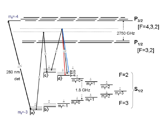
Figure 5.1: Schematic of relevant energy levels of one ²⁵Mg⁺ ion (not to scale). Shown are the ground-state hyperfine levels supplying the four ququat states ($|a\rangle$, $|b\rangle$, $|c\rangle$ and $|d\rangle$) and the harmonic oscillator levels due to the harmonic confinement in a trap similar to that described in [LBMW03]. We subsumed excited levels of the $P_{1/2}$ and $P_{3/2}$ states. Typically, the energy splitting of the motional levels and the Zeeman shift induced by an external magnetic field are of the same order of magnitude within 1-10 MHz, therefore much smaller than the hyperfine splitting of 1.8 GHz, the fine structure splitting of 2750 GHz and the optical transition frequency of the order of 1015 THz. We depict the resonant transition state sensitive detection and the two relevant types of two photon stimulated Raman transitions between states $|a\rangle\langle c|$ and $|c\rangle\langle d|$. The required transitions between states $|b\rangle\langle d|$ and $|a\rangle\langle b|$ would be provided by additional beams of slightly different frequencies or detunings.

At the start of each experiment, the ions will be laser cooled close to the motional ground state and optically pumped into state $|a\rangle$. Two carrier transitions and two red/blue side band transitions will be driven simultaneously to realize the calculation, one of each type depicted in Fig. 5.1. The coupling of states $|a\rangle\langle c|$ would be equivalent to that of the not shown $|b\rangle\langle d|$ via an additional carrier. The red/blue sideband transitions between $|a\rangle\langle b|$ would be driven by an additional pair of beams comparable but at slightly different frequencies or detunings to those shown driving $|c\rangle\langle d|$.

At the end of the calculation, state sensitive detection is to be realized by an additional laser beam, tuned to a cycling transition [LBMW03], coupling state $|a\rangle$ resonantly to the $P_{3/2}$ level. Since the Zeeman shift (1-10MHz) will not be sufficient in comparison to the line width of the resonant transition ($2p$ 43 MHz) to protect the population in state $|b\rangle$ against this interfering excitation, we will have to hide it in one of the $F=2$ ground state levels prior to detection. Thus, the population of state $|d\rangle$ would be transferred to state $|F=2,m_{f}=0\rangle$ to make room for the population of state $|b\rangle$ being transferred subsequently. To measure the population of any of the other three states we propose to use the carrier transition between states $|a\rangle\langle b|$ or $|c\rangle\langle d|$ instead of the side bands (and an additional carrier to drive $|a\rangle\langle c|$) to allow for the transfer into state $|a\rangle$. Since these carrier transitions do not affect the motional state populations, hiding the population of state $|c\rangle$ and driving a blue-sideband transition between the population transferred into state $|a\rangle$ and the cleared state $|c\rangle$ would allow for deriving the motional state population.

Taking into account the available laser intensities, all necessary Raman beams could be derived out of only one laser source. We would have to split the original beam and provide the necessary frequency offsets and switching via multi passing through acousto-optical modulators (AOM). The amount of necessary laser beams could be further reduced by using electro-optical modulators to provide red and blue sidebands at the same time. The additionally appearing carrier would just have to be book kept. There appear to be no fundamental reasons, why this experiment could not be realized with state of the art technology and fidelities of operation at the expense of only a slightly increased effort for the additionally required beams. We point out that, in order to facilitate the experiment, one could consider just the Dirac equation in 1+1 dimensions. The Hamiltonian to simulate in that case would have the form $H_{D}=c\sigma_{x}p_{x}+mc^{2}\sigma_{y}$, that could be easily implemented with one carrier, one blue- and one red-sideband transitions. We remark that the predictions of Dirac equation here reviewed, like Zitterbewegung, Klein’s paradox, Wigner rotations or mass acquisition would already take place at this level of 1+1 dimensions.

Part II Entanglement of continuous variables

Chapter 6 How much entanglement can be generated between two atoms by detecting photons?

In the world of quantum information processing it is widely accepted that, while photons are the ideal candidates for transmitting quantum information, this information is better stored and manipulated using atomic systems. The reason is that, while photons can be moved through long distances with little decoherence, atoms can be easily confined and can preserve quantum information for a long time. Consequently, an ideal design for a quantum network will conceivably be built upon a number of atomic or solid state devices which communicate through photonic quantum channels.

There exist mainly two methods for entangling distant atoms. The first one is based on emission of photons by the first atom, which afterwards interact with the second atom generating the entanglement [CZKM97, vECZ97, GST⁺98, PK00, CLE02, CLE03]. On the other hand, the second method relies on detecting the photons emitted by the two atoms with the subsequent entanglement generation due to interference in the measurement process [CCGFZ99, BKPV99]. Some aspects of these proposals have been experimentally verified [JKP01, KHR02, MBB⁺04, BMDM04, VWS⁺06, MCJ⁺06, MMM⁺06, CdF⁺05, DJD⁺05, BJD⁺06]. Most of the experiments with isolated atoms and light aim at entangling the internal state of the atom with the polarization of the photon [KHR02, MBB⁺04, BMDM04, VWS⁺06, MCJ⁺06, MMM⁺06]. It is clear that due to the size of the Hilbert space, the maximum attainable entanglement is one ebit.

In this chapter we will deal with the generation of entanglement between two atoms. We will focus on the second method mentioned above, in which entanglement is generated by measurements. To avoid the limit of one ebit, we work with continuous variables and seek entanglement in the motional state of the atoms. We will answer two fundamental questions: How much entanglement can be produced between the atoms? How can we achieve it? The basics of this chapter is contained in Ref. [LGRC07].

The first result, obtained in Section 6.1 is that by usual means —two atoms, one or two emitted photons, linear optics and postselection [CCGFZ99, MMM⁺06]—, we cannot produce more than 1 ebit of entanglement between the atoms, even if our Hilbert space is larger. The second result, exposed in Section 6.2 is that we can achieve an arbitrary amount of entanglement using at least two emitted photons and what we call an Entangling Two-Photon Detector (ETPD). The ETPD is a device which combines both photons in a projective measurement onto a highly entangled state. Theoretically, an ETPD could be built using a Kerr medium and postselection, but current nonlinear materials are too inefficient for such implementation. Inspired by the KLM proposal [KLM01], we demonstrate an efficient scheme for simulating the ETPD using ancillary photons. In Section 6.3 we clarify our proposal with a simple example: three photons and three detectors. Our last result, presented in Section 6.4 is that introducing $N-2$ additional photons in our setup, together with $N$ single-photon detectors, beam-splitters and an attenuator, we can obtain an amount of entanglement as high as $S=\log_{2}N$ ebits. Finally, at the end of the chapter we discuss the relevance of these results and possible implementations.

6.1 Entanglement based on atoms and photons

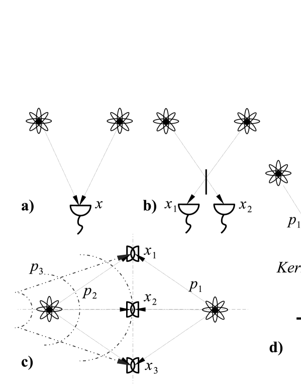
Figure 6.1: Schema of possible experiments for entangling two atoms. (a) Only one photon detected, but we do not know from which atom. (b) Two photons are detected, one from each atom. (c) Three photons are detected, one being supplied by the experiment (dashed line). Due to the setup, the probabilities of reaching each detector are balanced and the detectors do not distinguish between left- and right-coming photons. (d) Entangling Two-Photon Detector gedanken experiment. By detecting only a range of momenta we entangle the momenta of the atoms, $p_{1\perp}+p_{2\perp}\simeq 0$.

As mentioned above, current experiments with isolated atoms and light aim at entangling the internal state of the atom with the polarization of the photon [VWS⁺06]. It is clear that in both cases, due to the size of the Hilbert space, the maximum attainable entanglement is one ebit. We will rather work with continuous variables and seek entanglement between the motional state of the atom and the photon. We have in mind the setup in Ref. [CCGFZ99] where two atoms are excited with a very small probability and we consider the state of the atoms after spontaneous emission, when both are in the ground state. The state of the system is given by the wave function

$$|\Psi\rangle \sim \epsilon\int dp\,a^{\dagger}_{p}|\text{vac}\rangle({\cal G}_{1}(p)|-p,0\rangle+{\cal G}_{2}(p)|0,-p\rangle)+$$ (6.1)

$$+ \epsilon^{2}\int dp_{1}dp_{2}\,{\cal G}_{1}(p_{1}){\cal G}_{2}(p_{2})a^{\dagger}_{p1}a^{\dagger}_{p2}|\text{vac}\rangle|-p_{1},-p_{2}\rangle$$

$$+ |\text{vac}\rangle|0,0\rangle+{\cal O}(\epsilon^{3}).$$

Here $p$, $p_{1}$, $p_{2}$ denote the momenta of the emitted photons; $a_{p,p_{1},p_{2}}^{\dagger}$ their associated creation operators and $|\text{vac}\rangle$ the vacuum state of the EM field, and $\epsilon\ll 1$ is the excitation probability of the atoms. The initial momentum distribution of the emitted photons is given by ${\cal G}_{i}(p)$ for the $i$-th atom. As we will see later, we require some uncertainty in the initial momentum in order to generate a large amount of entanglement. Finally $|-p,0\rangle$, $|0,-p\rangle$ and $|-p_{1},-p_{2}\rangle$ denote the recoil momenta of the atoms after emitting the photons. The terms omitted in Eq. (6.1) correspond to higher order processes where an atom emits more than one photon. These terms will have a very small contribution if the decay time of the atom is longer than the duration of the exciting pulse.

Let us now consider a single detector placed symmetrically below the atoms [CCGFZ99], as in Fig. 6.1a. If there is one single photon detection, this will amount to a projective measurement onto a single-photon state and out of the state in Eq. (6.1) only the term on the first row will survive. Since the photons coming from the atoms are undistinguishable, an implicit symmetrization will take place and the final state of the atoms will be of the form $|\psi_{1}\rangle|0\rangle+|0\rangle|\psi_{2}\rangle$, for some motional states $\psi_{1}$ and $\psi_{2}$. Even though we work with continuous variables, this state can have at most 1 ebit which corresponds to $\langle{\psi_{1}|\psi_{2}}\rangle=\langle{\psi_{1}|0}\rangle=\langle{\psi_{2}|0}\rangle=0$.

We are going to show now that with two emitted photons, linear optics and two detectors, we cannot do better than one ebit of entanglement [See Fig. 6.1b]. The proof generalizes the previous argument with a little bit more care. First of all, linear optics amounts to a linear transformation of the initial momentum modes, $a_{p}$, to new operators, $b_{\gamma(p)}:=U_{\gamma}a_{p}U_{\gamma}^{\dagger}$. A trivial example of this is a $50\%$ beam splitter, which changes the photons from incident states $a_{+p}$ and $a_{-p}$ to $(a_{+p}\pm e^{i\phi}a_{-p})/\sqrt{2}$. Linear optics can be combined with measurements. Without loss of generality, all measurements will take place at the end of the process and they amount to a projection onto the modes $a_{x_{1}}$ and $a_{x_{2}}$ for the first and second detector, respectively. The state after a projective measurement onto two single-photon detectors reads

$$|\Psi_{\rm at}^{(2)}\rangle=\int dp_{1}dp_{2}{\cal G}_{1}(p_{1}){\cal G}_{2}(p_{2})\langle{a_{x_{1}}a_{x_{2}}b^{{\dagger}}_{\gamma_{1}(p_{1})}b^{{\dagger}}_{\gamma_{2}(p_{2})}}\rangle_{\text{vac}}|-p_{1},-p_{2}\rangle.$$ (6.2)

Note that the modes $a_{x_{1}}$ and $a_{x_{2}}$ detected by the first and second detector are expressed on an orthonormal basis different from that of the $a_{p}$ or $b$ operators. We enclose this information, plus the initial wavefunction of the photon in the following $c$-numbers

$$f_{j}(x_{i},p_{j}):={\cal G}_{j}(p_{j})[a_{x_{i}},b^{{\dagger}}_{\gamma_{j}(p_{j})}].$$ (6.3)

Using these wavefunctions we define the motional states

$$|\psi_{ij}\rangle:=\int dp\,f_{j}(x_{i},p)|p\rangle.$$ (6.4)

The expectation value in Eq. (6.2) can be written in terms of the $f_{j}(x_{i},p_{j})$. We thus arrive to the following expression for the atomic state after the measurement

$$|\Psi_{\rm at}^{(2)}\rangle\propto|\psi_{11}\rangle|\psi_{22}\rangle+|\psi_{21}\rangle|\psi_{12}\rangle.$$ (6.5)

This state cannot have more than 1 ebit of entanglement, which happens when all the states $\psi_{11}$, $\psi_{12}$, $\psi_{21}$ and $\psi_{22}$ are orthogonal to each other.

We must make several remarks. First of all, adding more detectors does not improve the outcome. Second, our proof is valid independently of the number of beam splitters, prisms, lenses and even polarizers we use. In particular, attenuating elements such as polarizers and filters can be treated as a linear operation plus a measurement and are covered by the previous formalism.

6.2 Arbitrary degree of entanglement between two atoms using postselection

We propose now to use an ETPD to obtain an arbitrary degree of entanglement between the two atoms. An ETPD is by definition a device that clicks whenever two photons arrive simultaneously and with their momenta satisfying a certain constraint. An example would be a parametric up-conversion crystal, in which pairs of photons with momenta $p_{1}$ and $p_{2}$ are converted with a certain probability into a new photon with momentum $p=p_{1}+p_{2}$. One imposes a constraint on the initial state by post-selecting a window of final momenta. For example, restricting the measurement to photons with transverse momentum $p_{\bot}=0$, then the initial contributing momenta must be those satisfying $p_{\bot 1}+p_{\bot 2}=0$ [Fig. 6.1d]. In this example the ETPD ideally projects the initial two photon product state $|\Psi^{0}_{\rm ph}\rangle\!\!=\!\!\!\int dp_{1}dp_{2}{\cal G}_{1}(p_{1}){\cal G}_{2}(p_{2})a^{{\dagger}}_{p_{1}}a^{{\dagger}}_{p_{2}}|{\rm vac}\rangle$ onto the probably entangled state

$$|\Psi^{\rm ETPD}_{\rm ph}\rangle\!\!=\!\!\!\int dp_{a}dp_{b}g(p_{a},p_{b})a^{{\dagger}}_{p_{a}}a^{{\dagger}}_{p_{b}}|{\rm vac}\rangle.$$ (6.6)

Here $g(p_{a},p_{b})$ is the acceptance function of the detector or, equivalently, the constraint that the final detected momenta $p_{a}$ and $p_{b}$ obey.

We claim now that with two emitted photons, linear operations and an ETPD, there is no limit to the attainable entanglement. To prove it we consider that after projection of the photon part of state in Eq. (6.1) into $|\Psi^{\rm ETPD}_{\rm ph}\rangle\!\!=\!\!\!\int dp_{a}dp_{b}g(p_{a},p_{b})a^{{\dagger}}_{p_{a}}a^{{\dagger}}_{p_{b}}|{\rm vac}\rangle$, the resulting atomic state will take the form

$$|\Psi_{\rm at}^{\rm ETPD}\rangle=\int dp_{a}dp_{b}\,g(p_{a},p_{b})|\Psi(p_{a},p_{b})\rangle$$ (6.7)

with the already entangled state

$$|\Psi(p_{a},p_{b})\rangle:=\int dp_{1}dp_{2}\,[f_{1}(p_{a},p_{1})f_{2}(p_{b},p_{2})+f_{1}(p_{b},p_{1})f_{2}(p_{a},p_{2})]|-p_{1},-p_{2}\rangle.$$ (6.8)

Depending on the specific shape of the functions $g(p_{a},p_{b})$ and $f_{i}(p_{l},p_{i})$ $l=a,b$, $i=1,2$, the corresponding state may reach an unbounded degree of entanglement. For example, let us consider that the photons evolve freely in space without any linear optics elements, $f_{i}(p,p_{i})={\cal G}_{i}(p_{i})\delta(p-p_{i})$, and assume that the detector has a very narrow acceptance function $g(p_{a},p_{b})=\delta(p_{a}+p_{b})$. The wider the initial momentum widths of the two photons, the larger the resulting bipartite atomic entanglement, which is not bounded from above. Indeed, in this ideal case the outcome will be much like the EPR pairs from the seminal paper Ref. [EPR35].

Current Kerr media are too inefficient to practically implement the ETPD introduced here. Motivated by this we have designed another protocol that simulates the outcome of an ETPD using linear optics, additional photons and postselection. As shown in the KLM proposal [KLM01], any highly entangling quantum gate can be performed this way. Some care is needed, though, because for our problem direct application of the KLM proposal results in a too large number of gates to even obtain a moderate amount of entanglement between both atoms.

Our proposal starts up from the two atoms after having emitted two photons, and we add $N-2$ additional ancillary photons,

$$|\Psi^{0}\rangle=\int dp_{1}dp_{2}...dp_{N}{\cal G}_{1}(p_{1}){\cal G}_{2}(p_{2})...{\cal G}_{N}(p_{N})a^{{\dagger}}_{p_{1}}a^{{\dagger}}_{p_{2}}...a^{{\dagger}}_{p_{N}}|{\rm vac}\rangle\otimes|-p_{1},-p_{2}\rangle.$$ (6.9)

The resulting state after linear operations on the $N$ photons, and $N$-fold coincidence count on the $N$ detectors, will be, analogously to the two-photon and two-detector case [Eqs. (6.2)-(6.5)]

$$|\Psi_{\rm at}^{(N)}\rangle=\sum_{(i_{1},...,i_{N})\in\Pi_{N}}\int dp_{1}...dp_{N}\prod_{k}f_{k}(x_{i_{k}},p_{k})|-p_{1},-p_{2}\rangle,$$ (6.10)

where $\Pi_{N}$ denotes the set of permutations of $N$ elements. This state may contain much more than one ebit of entanglement. In fact, an upper bound to the degree of attainable entanglement is $S=\log_{2}N$ ebits. We will show afterwards that this bound is indeed saturated.

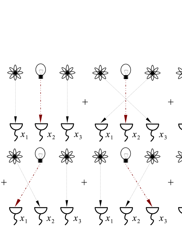
Figure 6.2: Outcome for an experiment with two atoms and three photons, as shown in Eq. (6.11).

6.3 Three photons and three detectors

As a clarifying example we consider the setup in Fig. 6.1c with three photons and three detectors. Photons $P1$ and $P_{2}$ come from their respective atoms, we introduce a single auxiliary photon, $P_{3}$ and we place three detectors symmetrically to the atoms, $X_{1}$, $X_{2}$, $X_{3}$. The final state for the two atoms, considering that all the three detectors are excited by the three photons, and fixing relative phases equal to 1 for simplicity purposes, would have the form

$$|\Psi_{\rm at}^{(3)}\rangle=\frac{1}{\sqrt{6}}(|1,2\rangle+|2,3\rangle+|3,1\rangle+|1,3\rangle+|3,2\rangle+|2,1\rangle),$$ (6.11)

where we denote with $|i,j\rangle$ the atomic state associated to detection of $P_{1}$ in $X_{i}$, and $P_{2}$ in $X_{j}$. In Fig. 6.2 we show the $N!=6$ processes that contribute coherently to the two-atom final entangled state. The previous state contains an entanglement of $S=1.25$ ebits.

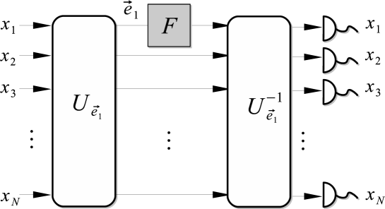
Figure 6.3: Quantum circuit for saturating the bound of $\log_{2}N$ ebits as described in the text.

6.4 Saturation of the entanglement bound $\log_{2}N$ ebits

The previous example is suboptimal. The maximal amount of entanglement of $S=\log_{2}N$ ebits is reachable for some of the states in Eq. (6.10). To prove it we consider a very symmetric configuration in which the detectors are located along a circle, equidistant to both atoms [Fig. 6.1c]. We will assume for simplicity that the two emitted photons and the $N-2$ ancillary ones are in $s$-wave states and arrive with equal probability and phase to every detector. In a similar fashion as in Eq. (6.11), the final bipartite atomic state will take the form

$$|\Psi_{\rm at}^{\rm sym}\rangle=\sum_{ij}C_{ij}|i,j\rangle\propto\sum_{ij}(1-\delta_{ij})|i,j\rangle,$$ (6.12)

where $|i,j\rangle$ is the final bipartite atomic state after detection of photon $P_{1}$ in detector $D_{i}$, and photon $P_{2}$ in detector $D_{j}$. In matrix form, the coefficients $C_{ij}$ are

$$C_{ij}\propto N\vec{e}_{1}(\vec{e}_{1})^{T}-I_{N\times N},$$ (6.13)

where $\vec{e}_{1}^{T}:=1/\sqrt{N}(1,1,...,1)_{N}$. Both the reduced density matrix of one atom and the Schmidt rank can be obtained from this matrix. The previous state can be rewritten in the form

$$C_{ij}\propto(N-1)\vec{e}_{1}(\vec{e}_{1})^{T}-\sum_{i=2}^{N}\vec{e}_{i}(\vec{e}_{i})^{T},$$ (6.14)

where $\{\vec{e}_{i}\}$, $i=2,...,N$ is a completion of $\vec{e}_{1}$ to an orthonormal basis in $\mathbf{C}^{N}$. From here it is obvious that the density matrix has full-rank and we can with local operations obtain a maximally entangled state of the form, up to local phases, $C_{ij}\propto I_{N\times N}$. To do so we must reduce the contribution of the term $\vec{e}_{1}$. As shown in Ref. [RZBB94], a network of beam-splitters and phase-shifters can be used to perform a unitary operation, $U_{\vec{e}_{1}}$, that maps the mode $a_{\vec{e}_{1}}\propto\sum_{i=1}^{N}a_{x_{i}}$ to a single optical port. If, as shown in Fig. 6.3 we place on that port a filter $F$ that decreases its amplitude by a factor $N-1$, when the $N$ detectors click simultaneously the atoms will get projected onto a maximally entangled state with $C_{ij}=\vec{e}_{1}(\vec{e}_{1})^{T}-\sum_{i=2}^{N}\vec{e}_{i}(\vec{e}_{i})^{T}.$ The proof is a little bit cumbersome, as it involves studying how all the photon modes in Eq. (6.9) transform under the nonunitary operation given by the network in Fig. 6.3 and then ensuring that the detection of $N$ photons does indeed give rise to the maximally entangled state. The state of the $N$ photons and $2$ atoms is given, before detection, by

$$|\Psi\rangle=(\sum_{j=1}^{N}a_{j}^{{\dagger}})^{N-2}\sum_{j_{1}=1}^{N}a_{j_{1}}^{{\dagger}}|j_{1}\rangle\sum_{j_{2}=1}^{N}a_{j_{2}}^{{\dagger}}|j_{2}\rangle|\rm vac\rangle,$$ (6.15)

where $|j_{i}\rangle$, $i=1,2$ is the recoil state of atom $i$, and $a_{j}$ is the mode associated to detector $j$. The linear transformation $U_{\vec{e}_{1}}$ applied to the modes before detection (see Fig.  6.3), maps the modes $a_{j}$ into the modes $c_{j}$, where $c_{1}^{{\dagger}}:=\sum_{j=1}^{N}a_{j}^{{\dagger}}$ and $c_{k}$, $k\neq 1$, are a completion to an orthonormal set, given by $c_{k}^{{\dagger}}:=\sum_{j=1}^{N}e_{kj}a_{j}^{{\dagger}}$. The corresponding state after application of $U_{\vec{e}_{1}}$ is

$$U_{\vec{e}_{1}}|\Psi\rangle=(c_{1}^{{\dagger}})^{N-2}\sum_{n_{1}=1}^{N}c_{n_{1}}^{{\dagger}}|e_{n_{1}}\rangle\sum_{n_{2}=1}^{N}c_{n_{2}}^{{\dagger}}|e_{n_{2}}\rangle|\rm vac\rangle,$$ (6.16)

where $|e_{n_{i}}\rangle$ is the recoil state of atom $i$ transformed under $U_{\vec{e}_{1}}$.

The following step of our protocol is the application of an attenuator $F$ to mode $c_{1}$, according to

$$c_{1}^{{\dagger}}\rightarrow\sqrt{1-p}+\sqrt{p}c_{1}^{{\dagger}}.$$ (6.17)

The meaning of Eq. (6.17) is clear: the attenuator absorbs the photon with a probability $1-p$ while leaves it unperturbed with a probability $p$. Postselection when detecting the $N$ photons will ensure that no photon has been absorbed in the process.

The resulting state is given by

$$FU_{\vec{e}_{1}}|\Psi\rangle=(c_{1}^{{\dagger}})^{N-2}\sqrt{p}^{N-2}\sum_{n_{1}=1}^{N}c_{n_{1}}^{{\dagger}}V_{n_{1}}|e_{n_{1}}\rangle\sum_{n_{2}=1}^{N}c_{n_{2}}^{{\dagger}}V_{n_{2}}|e_{n_{2}}\rangle|\rm vac\rangle,$$ (6.18)

where $V_{n_{i}}:=\sqrt{p}$ for $n_{i}=1$ and 1 otherwise.

Now we apply the inverse transformation $U_{\vec{e}_{1}}^{-1}$, giving

$$U_{\vec{e}_{1}}^{-1}FU_{\vec{e}_{1}}|\Psi\rangle=(\sum_{j=1}^{N}a_{j}^{{\dagger}})^{N-2}\sqrt{p}^{N-2}\sum_{n_{1}=1}^{N}\sum_{j_{1}=1}^{N}e_{n_{1}j_{1}}a_{j_{1}}^{{\dagger}}V_{n_{1}}|e_{n_{1}}\rangle\sum_{n_{2}=1}^{N}\sum_{j_{2}=1}^{N}e_{n_{2}j_{2}}a_{j_{2}}^{{\dagger}}V_{n_{2}}|e_{n_{2}}\rangle|\rm vac\rangle.$$

(6.19)

Upon detection of the $N$ photons at the $N$ detectors, the final atomic state will be

$$|\Psi_{\rm at}\rangle\propto\sum_{n_{1},n_{2}=1}^{N}\sum_{j_{1},j_{2}=1}^{N}C_{j_{1}j_{2}}e_{n_{1}j_{1}}e_{n_{2}j_{2}}V_{n_{1}}V_{n_{2}}|e_{n_{1}}e_{n_{2}}\rangle,$$ (6.20)

where $C_{j_{1}j_{2}}:=1-\delta_{j_{1}j_{2}}$ was previously introduced in (6.12) and appears due to the fact that each detector just clicks for one single photon. $C_{j_{1}j_{2}}$ may be recast in the form $C_{j_{1}j_{2}}=Ne_{1j_{1}}e_{1j_{2}}-\delta_{j_{1}j_{2}}$, producing an atomic state

$$|\Psi_{\rm at}\rangle\propto\sum_{n_{1},n_{2}=1}^{N}(V_{n_{1}}V_{n_{2}}N\delta_{1n_{1}}\delta_{1n_{2}}-V_{n_{1}}V_{n_{2}}\delta_{n_{1}n_{2}})|e_{n_{1}}e_{n_{2}}\rangle=\sum_{n=1}^{N}V_{n}^{2}(N\delta_{1n}-1)|e_{n}e_{n}\rangle.$$ (6.21)

On the other hand, we had that $V_{1}=\sqrt{p}$, and $V_{n}=1$ $n\neq 1$, so that our final result is that, fixing $p=\frac{1}{N-1}$ the final atomic state will be the maximally entangled state

$$|\Psi_{\rm at}\rangle\propto|e_{1}e_{1}\rangle-\sum_{n=2}^{N}|e_{n}e_{n}\rangle,$$ (6.22)

which contains an entanglement of $\log_{2}N$ ebits. This completes our proof.

Summing up, in this chapter we have demonstrated that it is possible to achieve an arbitrary amount of entanglement in the motional state of two atoms by using spontaneous emitted photons, linear optics and projective measurements. The resulting states can be used to study violation of Bell’s inequalities and also as a resource for quantum information processing. We expect that similar ideas can be used to entangle atomic clouds, replacing the photons with atoms, because in this case it is easy to build a two-atom detector.

Regarding the implementation, the ideas shown here can be tested easily in current experiments. We would suggest using two trapped ions as target atoms. The ions should be either on a very weak trap, or released right before excitation. The entanglement in the momentum will translate into an entanglement in the position of the atoms after a short time of flight. In practice, with only one additional photon, $1.58$ ebits can be produced, and we expect a value of $2$ ebits to be achievable. Clearly, due to the requirement of having single photons, producing a larger amount of entanglement will be more difficult with current technology, even though, as we have shown here, there is no fundamental limit.

Chapter 7 Spin entanglement loss by local correlation transfer to the momentum

Bipartite and multipartite entanglement is considered a basic resource in most applications of quantum information, communication, and technology  (see for instance Refs. [NC00, GMD02]). Entanglement is fragile, and it is well-known that in some cases interactions with an environment external to the entangled systems may decrease the quantum correlations, degrading this valuable resource [YE02, YE03, YE04, DH04, NS05, CMPB05, SMDZ06]. Momentum acts as a very special environment which every particle possesses and cannot get rid of. Consider for instance a bipartite system which initially is spin-entangled and with the momentum distributions factorized. It will decrease its spin-spin correlations provided any of the two particles entangles its spin with its momentum. This simple idea was studied in the natural framework of special relativity, where changing the reference frame induces Wigner rotations that entangle each spin with its momentum [PST02, Cza05, AM02, GA02, PS03, CW03, GBA03, LMDS06]. However, this is just a kinematical, frame-dependent effect only, and not a real dynamical interaction. On the other hand, this type of reasoning is also related to which-path detection [SZ97]. In addition, an experiment observing photon polarization disentanglement by correlation transfer, in this case to the photon’s position, was performed [SMKR01]. Can local interactions entangling spin with momentum produce the loss of non-local spin-spin entanglement? To our knowledge this question has not been explored in the literature. More remarkably, any particle owns a certain momentum distribution acting as an intrinsic environment, which can never be eliminated by improving the experimental conditions. But how does this fact affect the spin-spin correlations? This is the question we want to analyze [LLS06a] in this chapter.

In Section 7.1 we consider a bipartite system, composed by two $s=\frac{1}{2}$ fermions or two photons, which are initially in a Bell spin state $|\Psi^{-}\rangle$. We use a formalism that shows the decrease of spin entanglement whenever an interaction locally entangling spin with momentum takes place. We obtain the negativity $N$ [VW02] in terms of an integral depending on the spin rotation angle conditional to the momentum. In Section 7.2 we analyze this physical phenomenon in two specific situations: (i) Two spin-$\frac{1}{2}$ fermions in a $|\Psi^{-}\rangle$ Bell state, with Gaussian momentum distributions, that fly apart while one of them passes through a local magnetic field. Their spin entanglement decreases as a consequence of the transfer of correlations to the momentum of the latter fermion. And (ii) Two photons in a polarization $|\Psi^{-}\rangle$ Bell state, with Gaussian momentum distributions, which separate while one of them traverses an optically-active medium. This medium will entangle the polarization with the momentum and thus decrease the polarization entanglement. This is an unavoidable source of decoherence. In Section 7.3 we show that the apparent purely quantum communication resulting from these procedures is not possible. Classical communication has to be exchanged for the protocol to operate. The chapter ends with our conclusions.

7.1 Spin entanglement loss by correlation transfer to the momentum

We consider a maximally spin-entangled state for two $s=\frac{1}{2}$ fermions $A$ and $B$, or two photons $A$ and $B$. The case we analyze is that in which the two particles are far apart already. This avoids dealing with symmetrization issues. Indeed, our state is the maximally entangled one for two $s=\frac{1}{2}$ spins or polarizations, containing 1 ebit.

$$|\Psi^{-}_{\mathbf{p}}\rangle\!\!\! := \!\!\!\frac{1}{\sqrt{2}}[\Psi_{\uparrow}^{(\rm a)}(\mathbf{p_{a}})\Psi_{\downarrow}^{(\rm b)}(\mathbf{p_{b}})-\Psi_{\downarrow}^{(\rm a)}(\mathbf{p_{a}})\Psi_{\uparrow}^{(\rm b)}(\mathbf{p_{b}})],$$ (7.1)

where $\mathbf{p_{a}}$ and $\mathbf{p_{b}}$ are the corresponding momentum vectors of particles $A$ and $B$, and

$$\Psi_{\uparrow}(\mathbf{p}) := {\cal M}(\mathbf{p})|\!\!\uparrow\rangle=\left(\begin{array}[]{cccc}{\cal M}(\mathbf{p})\\ 0\\ \end{array}\right),$$ (7.4)

$$\Psi_{\downarrow}(\mathbf{p}) := {\cal M}(\mathbf{p})|\!\!\downarrow\rangle=\left(\begin{array}[]{cccc}0\\ {\cal M}(\mathbf{p})\\ \end{array}\right),$$ (7.7)

with bimodal momentum distribution ${\cal M}(\mathbf{p}):=\frac{1}{\sqrt{2}}(\delta_{\mathbf{p}\mathbf{p_{1}}}+\delta_{\mathbf{p}\mathbf{p_{2}}})$. We consider for the time being this kind of distribution for illustrative purposes. At the end of this section we generalize our results to arbitrary momentum distributions of the two particles. $|\!\!\uparrow\rangle$ and $|\!\!\downarrow\rangle$ represent either spin vectors pointing up and down along the $z$-axis, in the fermionic case, or right-handed and left-handed circular polarizations, in the photonic case. If we trace out the momentum degrees of freedom in Eq. (7.1), we obtain the usual spin Bell state, $|\Psi^{-}\rangle$.

We consider a local interaction which entangles the spin of each particle with its momentum through a real unitary (orthogonal) transformation $U$. We choose a real transformation for the sake of simplicity and in order to obtain fully analytical results. The generalization for inclusion of complex phases is straightforward but adds nothing of relevance in this section. We will take it fully into account in Sec. 7.2.

Each state vector in Eq. (7.7) transforms as

$$\Psi_{\uparrow}(\mathbf{p})=\left(\begin{array}[]{cccc}{\cal M}(\mathbf{p})\\ 0\\ \end{array}\right)\rightarrow$$ (7.10)

$$U[\Psi_{\uparrow}(\mathbf{p})]=\left(\begin{array}[]{cccc}\cos\theta_{\mathbf{p_{1}}}\\ \sin\theta_{\mathbf{p_{1}}}\\ \end{array}\right)\frac{\delta_{\mathbf{p}\mathbf{p_{1}}}}{\sqrt{2}}+\left(\begin{array}[]{cccc}\cos\theta_{\mathbf{p_{2}}}\\ \sin\theta_{\mathbf{p_{2}}}\\ \end{array}\right)\frac{\delta_{\mathbf{p}\mathbf{p_{2}}}}{\sqrt{2}},$$ (7.15)

$$\Psi_{\downarrow}(\mathbf{p})=\left(\begin{array}[]{cccc}0\\ {\cal M}(\mathbf{p})\\ \end{array}\right)\rightarrow$$ (7.18)

$$U[\Psi_{\downarrow}(\mathbf{p})]=\left(\begin{array}[]{cccc}-\sin\theta_{\mathbf{p_{1}}}\\ \,\,\,\,\,\cos\theta_{\mathbf{p_{1}}}\\ \end{array}\right)\frac{\delta_{\mathbf{p}\mathbf{p_{1}}}}{\sqrt{2}}+\left(\begin{array}[]{cccc}-\sin\theta_{\mathbf{p_{2}}}\\ \,\,\,\,\,\cos\theta_{\mathbf{p_{2}}}\\ \end{array}\right)\frac{\delta_{\mathbf{p}\mathbf{p_{2}}}}{\sqrt{2}},$$ (7.23)

where $\theta_{\mathbf{p_{1}}}$ and $\theta_{\mathbf{p_{2}}}$ produce a spin-momentum entangled state whenever $\theta_{\mathbf{p_{1}}}\neq\theta_{\mathbf{p_{2}}}$. The effect of this local interaction is that a part of the non-local spin-spin entanglement is transferred to the spin-momentum one, and the degree of entanglement of the spins decreases. To show this, we consider the state (7.1) evolved with the transformation $U$, and trace out the momenta.

$$\mathrm{Tr}_{\rm\mathbf{p_{a}},\mathbf{p_{b}}} (U|\Psi^{-}_{\mathbf{p}}\rangle\langle\Psi^{-}_{\mathbf{p}}|U^{{\dagger}})$$ (7.24)

$$= \frac{1}{2}\;\sum_{s,s^{\prime}}ss^{\prime}\mathrm{Tr}_{\rm\mathbf{p_{a}}}(U^{(\rm a)}[\Psi^{(\rm a)}_{s}(\mathbf{p_{a}})]\{U^{(\rm a)}[\Psi^{(\rm a)}_{s^{\prime}}(\mathbf{p_{a}})]\}^{{\dagger}})$$

$$\otimes\mathrm{Tr}_{\rm\mathbf{p_{b}}}(U^{(\rm b)}[\Psi^{(\rm b)}_{-s}(\mathbf{p_{b}})]\{U^{(\rm b)}[\Psi^{(\rm b)}_{-s^{\prime}}(\mathbf{p_{b}})]\}^{{\dagger}}),$$

where $ss^{\prime}:=\delta_{s,s^{\prime}}-\delta_{s,-s^{\prime}}$. It can be appreciated in Eq. (7.24) that the expression is decomposable in sum of tensor products of 2$\times$2 spin blocks, each corresponding to each particle. We compute now the different blocks, corresponding to the four possible tensor products of the states (7.23)

$$\mathrm{Tr}_{\rm\mathbf{p}}[U\Psi_{\uparrow}(U\Psi_{\uparrow})^{{\dagger}}] = \frac{1}{2}\left(\begin{array}[]{cc}c_{1}^{2}+c_{2}^{2}&c_{1}s_{1}+c_{2}s_{2}\\ c_{1}s_{1}+c_{2}s_{2}&s_{1}^{2}+s_{2}^{2}\end{array}\right),$$ (7.27)

$$\mathrm{Tr}_{\rm\mathbf{p}}[U\Psi_{\uparrow}(U\Psi_{\downarrow})^{{\dagger}}] = \frac{1}{2}\left(\begin{array}[]{cc}-c_{1}s_{1}-c_{2}s_{2}&c_{1}^{2}+c_{2}^{2}\\ -s_{1}^{2}-s_{2}^{2}&c_{1}s_{1}+c_{2}s_{2}\end{array}\right),$$ (7.30)

$$\mathrm{Tr}_{\rm\mathbf{p}}[U\Psi_{\downarrow}(U\Psi_{\uparrow})^{{\dagger}}] = \frac{1}{2}\left(\begin{array}[]{cc}-c_{1}s_{1}-c_{2}s_{2}&-s_{1}^{2}-s_{2}^{2}\\ c_{1}^{2}+c_{2}^{2}&c_{1}s_{1}+c_{2}s_{2}\end{array}\right),$$ (7.33)

$$\mathrm{Tr}_{\rm\mathbf{p}}[U\Psi_{\downarrow}(U\Psi_{\downarrow})^{{\dagger}}] = \frac{1}{2}\left(\begin{array}[]{cc}s_{1}^{2}+s_{2}^{2}&-c_{1}s_{1}-c_{2}s_{2}\\ -c_{1}s_{1}-c_{2}s_{2}&c_{1}^{2}+c_{2}^{2}\end{array}\right),$$ (7.36)

where $c_{i}:=\cos(\theta_{\mathbf{p_{i}}})$ and $s_{i}:=\sin(\theta_{\mathbf{p_{i}}})$. This way, it is possible to compute the effects of the local interaction $U$ in the state $|\Psi^{-}_{\mathbf{p}}\rangle$ after tracing out the momentum. We choose equal interaction angles for the two particles, $\theta_{\mathbf{p_{i}}}^{(\rm a)}=\theta_{\mathbf{p_{i}}}^{(\rm b)}$, as a natural simplification. The resulting bipartite spin state is

$$\left(\!\!\!\begin{array}[]{cccc}\frac{1}{4}s_{12}^{2}&0&0&\frac{1}{4}s_{12}^{2}\\ 0&\frac{1}{4}(1+c_{12}^{2})&-\frac{1}{4}(1+c_{12}^{2})&0\\ 0&-\frac{1}{4}(1+c_{12}^{2})&\frac{1}{4}(1+c_{12}^{2})&0\\ \frac{1}{4}s_{12}^{2}&0&0&\frac{1}{4}s_{12}^{2}\\ \end{array}\!\!\!\right),\\$$ (7.37)

where $s_{12}:=\sin(\theta_{\mathbf{p_{1}}}-\theta_{\mathbf{p_{2}}})$ and $c_{12}:=\cos(\theta_{\mathbf{p_{1}}}-\theta_{\mathbf{p_{2}}})$. The entanglement measure we will use is the negativity [VW02], defined as $N:=\max\{0,-2\lambda_{\rm min}\}$, where $\lambda_{\rm min}$ is the smallest eigenvalue of the partial transpose (PT) matrix of Eq. (7.37). It is very easily computable, and is found to be

$$N=\cos^{2}(\theta_{\mathbf{p_{1}}}-\theta_{\mathbf{p_{2}}}).$$ (7.38)

From this expression it can be appreciated that for $\theta_{\mathbf{p_{1}}}=\theta_{\mathbf{p_{2}}}$ the entanglement remains maximal (1 ebit), and for $\theta_{\mathbf{p_{1}}}$ separating from $\theta_{\mathbf{p_{2}}}$ the entanglement decreases, until $\theta_{\mathbf{p_{1}}}-\theta_{\mathbf{p_{2}}}=\pi/2$, where it vanishes and the state becomes separable. We plot this behavior in Figure 7.1, showing the negativity $N$ in Eq. (7.38) as a function of $\theta_{\mathbf{p_{1}}}$ and $\theta_{\mathbf{p_{2}}}$. Every local interaction producing spin-momentum entanglement will in general diminish the initial maximal spin-spin entanglement of the two particles, thus degrading this resource. This result is valid either for $s=\frac{1}{2}$ fermions or photons, as they both have a two-dimensional internal Hilbert space.

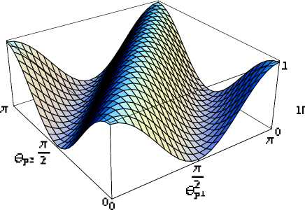
Figure 7.1: Negativity $N$ in Eq. (7.38) as a function of $\theta_{\mathbf{p_{1}}}$ and $\theta_{\mathbf{p_{2}}}$.

The generalization of Eq. (7.38) to a uniform distribution with $n$ different momenta is straightforward, and the spectrum of the corresponding PT matrix is

$$\sigma_{\rm PT}=\left\{\frac{1}{2},\frac{1}{2},\pm\left[\frac{1}{2}-\frac{1}{n^{2}}\sum_{i,j=1}^{n}\cos^{2}(\theta_{\mathbf{p_{i}}}-\theta_{\mathbf{p_{j}}})\right]\right\},$$ (7.39)

with a resulting negativity

$$N=\left|1-\frac{2}{n^{2}}\sum_{i,j=1}^{n}\cos^{2}(\theta_{\mathbf{p_{i}}}-\theta_{\mathbf{p_{j}}})\right|.$$ (7.40)

We take now the continuous limit, for an arbitrary momentum distribution $\tilde{\psi}(\mathbf{p})$ for each particle. We suppose for the sake of simplicity $|\tilde{\psi}^{(\rm a)}(\mathbf{p})|=|\tilde{\psi}^{(\rm b)}(\mathbf{p})|$, although the spatial distributions do not overlap, as the two particles are far away. Accordingly, $N$ will be

$$N=\left|1-2\int d^{3}\mathbf{p}\int d^{3}\mathbf{p^{\prime}}|\tilde{\psi}(\mathbf{p})|^{2}|\tilde{\psi}(\mathbf{p^{\prime}})|^{2}\cos^{2}(\theta_{\mathbf{p}}-\theta_{\mathbf{p^{\prime}}})\right|.$$ (7.41)

Notice that this expression involves an integration over the momentum variables $\mathbf{p}$ and $\mathbf{p^{\prime}}$, associated to the same particle (not to each of them). We point out that, according to (7.41), in the case where momentum does not entangle with spin (i.e. whenever $\theta_{\mathbf{p}}$ is a constant), then $N=1$ and thus the spin-spin entanglement remains maximal. Otherwise, the spin-spin entanglement would decrease due to the transfer of correlations to the spin-momentum part.

The loss of spin entanglement under a spin-momentum entangling transformation can take place in a variety of possible situations. Wigner rotations that appear under relativistic change of reference frame entangle each spin with its momentum producing loss of spin-spin entanglement [PST02, Cza05, AM02, GA02, PS03, CW03, GBA03, LMDS06]. This is just a kinematical-relativistic effect, not due to a dynamical interaction. In the rest of the chapter we focus on two relevant examples of these interactions, taking fully into account the complex phases: a local homogeneous magnetic field, for the two-fermion case, and a local optically-active medium, for the two-photon case.

7.2 Applications

7.2.1 Two fermions and a local magnetic field

In this section we analyze a bipartite system, composed by two $s=\frac{1}{2}$ neutral fermions $A$ and $B$, which are initially far apart and in a Bell spin state $|\Psi^{-}\rangle$, with factorized Gaussian momentum distributions. We consider that one of them traverses a region where a finite, homogeneous magnetic field exists. As a result, it will transfer part of its spin correlations to the momentum.

The initial spin-entangled state for the two fermions $A$ and $B$ is

$$|\Psi^{-}_{\mathbf{p}}\rangle\!\!\! := \!\!\!\frac{1}{\sqrt{2}}[\Psi_{\uparrow}^{(\rm a)}(\mathbf{p_{a}})\Psi_{\downarrow}^{(\rm b)}(\mathbf{p_{b}})-\Psi_{\downarrow}^{(\rm a)}(\mathbf{p_{a}})\Psi_{\uparrow}^{(\rm b)}(\mathbf{p_{b}})],$$ (7.42)

where $\mathbf{p_{a}}$ and $\mathbf{p_{b}}$ are the corresponding momentum vectors of particles $A$ and $B$, and

$$\Psi_{\uparrow}(\mathbf{p}) := {\cal G}(\mathbf{p})|\!\!\uparrow\rangle=\left(\begin{array}[]{cccc}{\cal G}(\mathbf{p})\\ 0\\ \end{array}\right),$$ (7.45)

$$\Psi_{\downarrow}(\mathbf{p}) := {\cal G}(\mathbf{p})|\!\!\downarrow\rangle=\left(\begin{array}[]{cccc}0\\ {\cal G}(\mathbf{p})\\ \end{array}\right),$$ (7.48)

with Gaussian momentum distribution ${\cal G}(\mathbf{p}):=\pi^{-3/4}\sigma^{-3/2}\exp[-(\mathbf{p}-\mathbf{p}_{0})^{2}/2\sigma^{2}]$. In Eqs. (7.48) we are not indicating explicitly the particle index. In the center of mass frame, $\mathbf{p}^{(\rm b)}_{0}=-\mathbf{p}^{(\rm a)}_{0}$, and we consider that the two particles are flying apart from each other. $|\!\!\uparrow\rangle$ and $|\!\!\downarrow\rangle$ represent spin vectors pointing up and down along the $z$-axis, respectively. If we trace out momentum degrees of freedom in Eq. (7.42), we obtain the usual spin Bell state, $|\Psi^{-}\rangle$.

Suppose a local interaction which entangles the spin of fermion $A$ with its momentum through a unitary transformation $U$. In this case we choose a magnetic field $\mathbf{B}_{0}$ which is constant on a bounded region $\cal{D}$ of length $L$, along the direction of $\mathbf{p}^{(\rm a)}_{0}$, vanishes outside $\cal{D}$, and extends infinitely with a constant value along the other two orthogonal directions, as shown in Figure 7.2. We take $\mathbf{B}_{0}$ along the direction orthogonal to $\mathbf{p}^{(\rm a)}_{0}$, so it is divergenceless, $\mathbf{\nabla}\cdot\mathbf{B}_{0}=0$, and we quantize the spin along $\mathbf{B}_{0}$ so that $\mathbf{\sigma}\cdot\mathbf{B}_{0}=sB_{0}$, with $s$ the corresponding spin component. Due to the rotational invariance of the spin singlet, this choice is completely general. In momentum space, the problem reduces to one dimension, the one associated to the direction of $\mathbf{p}^{(\rm a)}_{0}$. We will denote from now on $p$ to the corresponding momentum coordinate.

Figure 7.2: Sketch of the two-fermion case explained in the text. Fermion $A$ traverses a constant magnetic field $\mathbf{B}_{0}$ located in region $\cal{D}$ with a width $L$ along the direction of $\mathbf{p}^{(\rm a)}_{0}$.

The system Hamiltonian can be written as

$$H\,=\,\frac{\mathbf{p}^{2}}{2m}\,+\,\gamma\,(\mathbf{B}_{0}\cdot\mathbf{S})\,\theta(x)\,\theta(L-x),$$ (7.49)

where $\gamma$ is the magnetic moment of our neutral particle. Accordingly, we get

$$\dot{\mathbf{p}}\,=\,i[H,\mathbf{p}] = \left(-\gamma\,(\mathbf{B}_{0}\cdot\mathbf{S})\,[\delta(x)-\delta(L-x)],0,0\right),$$ (7.50)

$$\dot{\mathbf{S}}\,=\,i[H,\mathbf{S}] = -\gamma\,(\mathbf{B_{0}}\wedge\mathbf{S})\,\theta(x)\,\theta(L-x),$$

$$\ddot{\mathbf{S}}\,=\,i[H,\dot{\mathbf{S}}] = -\gamma\,\left[(\mathbf{B_{0}}\cdot\mathbf{S})\,\mathbf{B_{0}}-\mathbf{B_{0}}^{2}\mathbf{S}\right]\theta(x)\,\theta(L-x)$$

$$-\,i\gamma\,(\mathbf{B_{0}}\wedge\mathbf{S})\left(\frac{\mathbf{p}}{m}[\mathbf{p},(\delta(x)-\delta(L-x))]\right).$$

From the first of the above equations we obtain $\frac{\partial}{\partial x}(p^{2}/2m)=-\gamma\,(\mathbf{B_{0}}\cdot\mathbf{S})\left[\delta(x)-\delta(L-x)\right]$ like using matching conditions at $x=0,L$. The second and third equations give the spin evolution. By inspection we see that i) the spin remains parallel to $\mathbf{B_{0}}$ if it was initially so and, ii) the spin is constant in this case $\dot{\mathbf{S}}\,=\,\ddot{\mathbf{S}}\,=\,0$. Hence, in spite of choosing a case where the spin is conserved, its entanglement with the momentum decreases the spin correlations with the idle fermion.

The effect of the magnetic field on particle $A$ can be seen in its state. Behind the region $\cal{D}$, the resulting state vector as transformed from the one in Eq. (7.48) is

$$\Psi_{\uparrow}(\mathbf{p})\rightarrow U[\Psi_{\uparrow}(\mathbf{p})]={\cal{T}}_{\uparrow}(p)\left(\begin{array}[]{cccc}{\cal G}(\mathbf{p})\\ 0\\ \end{array}\right),$$ (7.53)

$$\Psi_{\downarrow}(\mathbf{p})\rightarrow U[\Psi_{\downarrow}(\mathbf{p})]={\cal{T}}_{\downarrow}(p)\left(\begin{array}[]{cccc}0\\ {\cal G}(\mathbf{p})\\ \end{array}\right),$$ (7.56)

where ${\cal{T}}_{\uparrow}(p)$ (${\cal{T}}_{\downarrow}(p)$) is the transmission coefficient associated to the mesa (well) potential induced by $\mathbf{B}_{0}$, for initial spin up (down). It is given by

$${\cal{T}}_{s}(p):=\frac{2pp_{s}e^{-ipL}}{2pp_{s}\cos(p_{s}L)-i(p^{2}+p_{s}^{2})\sin(p_{s}L)},$$ (7.57)

where $p_{s}(p,B_{0}):=\sqrt{p^{2}-2sm\gamma B_{0}}$, as given by (7.50), $B_{0}:=|\mathbf{B_{0}}|$ and $s=\frac{1}{2}(-\frac{1}{2})$ for spin $\uparrow(\downarrow)$. As expected for $B_{0}=0$, ${\cal{T}}_{\uparrow}(p)={\cal{T}}_{\downarrow}(p)=1$. The initial state is preserved so no spin-momentum correlations are generated. In general, for $B_{0}\neq 0$, ${\cal{T}}_{\uparrow}(p)\neq{\cal{T}}_{\downarrow}(p)$, producing spin-momentum entanglement. We are considering here just transmission through the region $\cal{D}$, without taking into account the reflection of the wave packets. We suppose all the measurements will take place beyond $\cal{D}$ so we may normalize the final transmitted state to 1. Finally, the net effect of this local interaction is the reshuffling of spin-momentum correlations in the state of the active fermion. Accordingly, the degree of spin-spin entanglement between both particles decreases. As was done in Eq. (7.24), we evolve the state (7.42) with the transformation $U$ and trace out the momenta

$$\mathrm{Tr}_{\rm\mathbf{p_{a}},\mathbf{p_{b}}} (U|\Psi^{-}_{\mathbf{p}}\rangle\langle\Psi^{-}_{\mathbf{p}}|U^{{\dagger}})$$ (7.58)

$$= \!\!\!\!\!\!\frac{1}{2}\sum_{s,s^{\prime}}ss^{\prime}\mathrm{Tr}_{\rm\mathbf{p_{a}}}(U[\Psi^{(\rm a)}_{s}(\mathbf{p_{a}})]\{U[\Psi^{(\rm a)}_{s^{\prime}}(\mathbf{p_{a}})]\}^{{\dagger}})$$

$$\otimes\mathrm{Tr}_{\rm\mathbf{p_{b}}}(\Psi^{(\rm b)}_{-s}(\mathbf{p_{b}})\{\Psi^{(\rm b)}_{-s^{\prime}}(\mathbf{p_{b}})\}^{{\dagger}}),$$

where $ss^{\prime}:=\delta_{s,s^{\prime}}-\delta_{s,-s^{\prime}}$. The traces corresponding to particle $B$ give just the initial spin states, $|\!\!\!\downarrow\rangle\langle\downarrow\!\!\!|$, $|\!\!\!\uparrow\rangle\langle\uparrow\!\!\!|$, $|\!\!\!\downarrow\rangle\langle\uparrow\!\!\!|$, $|\!\!\!\uparrow\rangle\langle\downarrow\!\!\!|$, because $U$ is just the identity for $B$. The resulting, properly normalized spin-spin state is

$$\left(\!\!\!\begin{array}[]{cccc}0&0&0&0\\ 0&I_{\uparrow\uparrow}&-I_{\uparrow\downarrow}&0\\ 0&-I_{\downarrow\uparrow}&I_{\downarrow\downarrow}&0\\ 0&0&0&0\\ \end{array}\!\!\!\right),\\$$ (7.59)

where

$$I_{ss^{\prime}}:=\int d^{3}\mathbf{p}|{\cal{G}}(\mathbf{p})|^{2}\frac{{\cal{T}}_{s}(p){\cal{T}}^{*}_{s^{\prime}}(p)}{|{\cal{T}}_{\uparrow}(p)|^{2}+|{\cal{T}}_{\downarrow}(p)|^{2}}.$$ (7.60)

The negativity for this state is found to be

$$N=2|I_{\uparrow\downarrow}|\geq 0.$$ (7.61)

This expression for $N$ is rather illuminating and its behavior easy to understand. For the initial state (7.42) $N=1$ (1 initial ebit), and, as long as the magnetic field is increased, ${\cal{T}}_{\uparrow}(p)$ and ${\cal{T}}_{\downarrow}(p)$ become more different, making the term $I_{\uparrow\downarrow}$ smaller, and diminishing $N$.

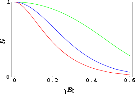
Figure 7.3: Negativity $N$ in Eq. (7.61) as a function of $\gamma B_{0}$ for $m=100$, $p^{(\rm a)}_{0}=10$, $L=3$, and $\sigma^{(\rm a)}=1$, 2, and 3. The higher curves corresponds to the thinner $\sigma$’s. All quantities are measured with respect to a global arbitrary energy scale.

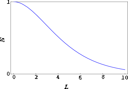
Figure 7.4: Negativity $N$ in Eq. (7.61) as a function of $L$ for $m=100$, $p^{(\rm a)}_{0}=10$, $\gamma B_{0}=0.2$, and $\sigma^{(\rm a)}=2$. All quantities are measured with respect to a global arbitrary energy scale.

On the other hand, the wider $\sigma^{(\rm a)}$ the more destructive interference between ${\cal{T}}_{\uparrow}(p)$ and ${\cal{T}}_{\downarrow}(p)$ will occur, reducing $N$. We plot in Figure 7.3 the negativity $N$ as a function of $\gamma B_{0}$, with $B_{0}:=|\mathbf{B}_{0}|$, for $m=100$, $p^{(\rm a)}_{0}:=|\mathbf{p}^{(\rm a)}_{0}|=10$, $L=3$, and $\sigma^{(\rm a)}=1$, 2, and 3. All quantities are measured with respect to a global arbitrary energy scale. The entanglement goes to zero with increasing $B_{0}$, and the wider $\sigma^{(\rm a)}$, the lesser the entanglement. A similar behaviour arises from the cumulative effect of the barrier; the larger $L$, the smaller the entanglement. We show in Figure 7.4 this behavior, plotting $N$ as a function of $L$ for $m=100$, $p^{(\rm a)}_{0}=10$, $\gamma B_{0}=0.2$, and $\sigma^{(\rm a)}=2$.

7.2.2 Two photons and an optically-active medium

In this section we analyze a bipartite system, composed by two photons $A$ and $B$, which are far apart in a polarization Bell state $|\Psi^{-}\rangle$ with factorized Gaussian momentum distributions. We consider that the photon $A$ traverses a region where a finite, optically-active medium, exists. As a result, part of its spin correlations will be transferred to the momentum.

Basically the mathematical formalism used for the two-fermion case is also valid here, with $\uparrow$ and $\downarrow$ indicating right-hand and left-hand circular polarizations, which we will denote by R and L indices. The transmission coefficient in the WKB approximation, at lowest order, takes now the form of a complex phase, depending on the polarization

$${\cal{T}}_{s}(w):=\exp[iwn_{s}(w)L],\;\;\;s=R,L,$$ (7.62)

where the refractive indices are

$$n_{\rm R,L}(w):=\sqrt{1+\chi_{11}\pm\chi_{12}},$$ (7.63)

and $\chi_{11}$, $\chi_{12}$ are two of the matrix elements of the susceptibility $\chi$,

$$\chi:=\left(\begin{array}[]{ccc}\chi_{11}&i\chi_{12}&0\\ -i\chi_{12}&\chi_{11}&0\\ 0&0&\chi_{33}\end{array}\right).$$ (7.64)

$\chi$ is produced, for example, by an isotropic dielectric placed in a magnetic field $\mathbf{B}_{0}$ directed along $z$, which is also the direction of photon propagation. $L$ is the dielectric length that the photon traverses. $\chi_{11}$ and $\chi_{12}$ are

$$\chi_{11}(w):=\frac{{\cal{N}}e^{2}}{m\epsilon_{0}}\left[\frac{w_{0}^{2}-w^{2}}{(w_{0}^{2}-w^{2})^{2}-w^{2}w_{c}^{2}}\right],$$

$$\chi_{12}(w):=\frac{{\cal{N}}e^{2}}{m\epsilon_{0}}\left[\frac{ww_{c}}{(w_{0}^{2}-w^{2})^{2}-w^{2}w_{c}^{2}}\right],$$ (7.65)

where the cyclotron frequency $w_{c}:=e|\mathbf{B}_{0}|/m$, $e$ is the electron charge, $m$ its mass, $w_{0}$ the resonance frequency of the optically-active medium, ${\cal{N}}$ the number of electrons per unit volume, and $\epsilon_{0}$ the vacuum electric permittivity.

The next order correction would include factors $\sqrt{n_{\rm R,L}}$ in the denominators of the transmission coefficients. However, the approximation that considers these factors coincides exactly with the lowest order one when taking into account just linear terms in $\mathbf{B}_{0}$. We will consider the realistic case in which $w_{c}$ is small as compared to the photon average energy. Thus we will work from the very beginning just with the transmission coefficients (7.62).

The negativity $N$, obtained for this case in analogy with the two-fermion case, is

$$N\simeq\frac{1}{\sqrt{\pi}\sigma}\left|\int_{0}^{\infty}dwe^{-(w-p_{0})^{2}/\sigma^{2}}e^{i\tilde{B}L\frac{w^{2}}{(w^{2}-w_{0}^{2})^{2}}}\right|,$$ (7.66)

where $p_{0}$ is the average momentum of photon $A$, $\sigma\ll p_{0}$ its momentum width, and $\tilde{B}:={\cal N}e^{3}|\mathbf{B}_{0}|/(m^{2}\epsilon_{0})$.

We plot in Figure 7.5 the negativity $N$ in Eq. (7.66) as a function of $\tilde{B}L$ for $p_{0}=10$, $\sigma=2$, and $w_{0}=10$. All quantities are measured with respect to a global arbitrary energy scale. The entanglement decreases as the magnetic field $\tilde{B}$ or the length $L$ of the dielectric increase. We plot also in Figure 7.6 the negativity $N$ as a function of $\sigma$ for $p_{0}=10$, $\tilde{B}L=4$, and $w_{0}=10$. Surprisingly, and opposite to the two-fermion case, the entanglement increases as the momentum width $\sigma$ of the photon is larger. This effect comes from the fact that for larger widths, centered at $w_{0}$, the contribution from the region around the resonance frequency $w_{0}$, in which the effect of the medium is appreciable, becomes smaller. On the other hand, in the limit of negligible width, the spin could not get entangled with the momentum so in this limit the spin-spin entanglement would remain maximal. We observe then that there is a region of intermediate widths $\sigma$ in which the spin-spin entanglement becomes minimal. Finally, we plot in Figure 7.7 the negativity $N$ as a function of $w_{0}$ for $p_{0}=10$, $\tilde{B}L=2$, and $\sigma=0.5,1,2$. The larger $\sigma$ corresponds in this figure to the higher curves. These graphics show that the entanglement decreases mainly for resonance frequencies $w_{0}$ around the average momentum $p_{0}$. It also shows the surprising behavior mentioned above: For wider $\sigma$, the entanglement is larger, and the interval of $w_{0}$ for which the entanglement decreases is wider, as expected according to the previous analysis.

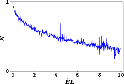
Figure 7.5: Negativity $N$ in Eq. (7.66) as a function of $\tilde{B}L$ for $p_{0}=10$, $\sigma=2$, and $w_{0}=10$. All quantities are measured with respect to a global arbitrary energy scale.

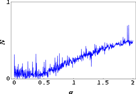
Figure 7.6: Negativity $N$ in Eq. (7.66) as a function of $\sigma$ for $p_{0}=10$, $\tilde{B}L=4$, and $w_{0}=10$. All quantities are measured with respect to a global arbitrary energy scale.

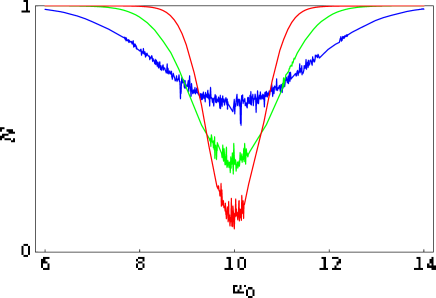
Figure 7.7: Negativity $N$ in Eq. (7.66) as a function of $w_{0}$ for $p_{0}=10$, $\tilde{B}L=2$, and $\sigma=0.5,1,2$. The larger $\sigma$ corresponds to the higher curves. All quantities are measured with respect to a global arbitrary energy scale.

7.3 Is purely quantum communication feasible?

A cautious reader may immediately object that, in principle, our preceding analysis seems to suggest the feasibility of communication through a purely quantum channel, i.e. without classical communication, as in all quantum-informational protocols. Let us illustrate this point with the following proposal based in the previous two-fermion case. As usual, Alice and Bob will be the corresponding observers of each fermion. The joint spin-spin state is given by equation (7.59), which immediately drives one to the subsequent reduced spin state for fermion $B$:

$$\rho_{B}=\begin{pmatrix}I_{\downarrow\downarrow}&0\\ 0&I_{\uparrow\uparrow}\end{pmatrix}.$$ (7.67)

But the quantities $I_{ss^{\prime}}$ depend on the magnetic field $B_{0}$ (cf. equations (7.60) and (7.57)), which can be controlled by Alice. This allows them to agree on the following procedure. They agree on communicating with a binary alphabet with classical bits $0$ and $1$. If Alice were to communicate $0$, she would adjust $B_{0}$ so that the reduced spin state for Bob is, for example,

$$\rho_{B}^{(0)}=\begin{pmatrix}\frac{3}{4}&0\\ 0&\frac{1}{4}\end{pmatrix}.$$ (7.68)

They prepare a statistically significative amount of pairs of fermions under such conditions. Then Bob, when measuring the spin upon his fermion, will typically obtain spin up in the $75\%$ of the measurements and spin down in the remaining $25\%$. He thus deduces that Alice is sending the bit $0$. On the contrary, if Alice were to communicate the bit $1$, she would adjust $B_{0}$ so that the reduced spin state for Bob is, for example,

$$\rho_{B}^{(1)}=\begin{pmatrix}\frac{1}{4}&0\\ 0&\frac{3}{4}\end{pmatrix}.$$ (7.69)

They also prepare a statistically significative amount of pairs and Bob perfoms his measurements. He will detect $75\%$ of them in the spin down state and $25\%$ in the spin up state. He thus deduces that Alice is sending the bit $1$. Notice that this information transmission is carried out without the assistance of classical communication.

The flaw stems from the disregarding of the wave packet reflection in Alice’s site. This can be seen in two complementary ways. On one hand, to perform a genuine information transmission in which Bob’s fermion is actually carrying information encoded by Alice, he must be able to discern between those fermions whose pairs have been reflected in Alice’s barrier potential, so that he can securely discard them (they are not carrying information at all). And this is only possible if Alice classically communicates this information to Bob.

On the other hand, a detailed calculation taking into account the reflection coefficients, hence without the normalization appearing in the denominator of (7.60), shows that Bob’s reduced spin state will be given by:

$$\rho_{B} = \frac{1}{2}\begin{pmatrix}\int d^{3}\mathbf{p}|\mathcal{G}(\mathbf{p})|^{2}|\mathcal{R}_{\downarrow}(p)|^{2}&0\\ 0&\int d^{3}\mathbf{p}|\mathcal{G}(\mathbf{p})|^{2}|\mathcal{R}_{\uparrow}(p)|^{2}\end{pmatrix}$$ (7.70)

$$+ \frac{1}{2}\begin{pmatrix}\int d^{3}\mathbf{p}|\mathcal{G}(\mathbf{p})|^{2}|\mathcal{T}_{\downarrow}(p)|^{2}&0\\ 0&\int d^{3}\mathbf{p}|\mathcal{G}(\mathbf{p})|^{2}|\mathcal{T}_{\uparrow}(p)|^{2}\end{pmatrix}=$$

$$= \frac{1}{2}\begin{pmatrix}1&0\\ 0&1\end{pmatrix},$$

where $\mathcal{R}_{s}(p)$ denotes the corresponding reflection coefficient for spin $s$ and momentum $p$. The calculation reveals that Bob gains no information whatsoever from Alice’s decisions, unless she classically informs Bob about them. Mathematically this can be expressed through the unitary character of the process. If no classical information is exchanged, the evolution is locally unitary ($\Psi^{(a)}\otimes\Psi^{(b)}\to U^{(a)}[\Psi^{(a)}]\otimes U^{(b)}[\Psi^{(b)}]$) and thus cannot change the entanglement shared by both parties (the entanglement class is invariant under locally unitary evolution). Consequently no information through the purely quantum channel can be obtained. On the contrary, if Alice classically sends information to Bob, she is actually selecting a subset of her incoming fermions, i.e. she is projecting her state ($\Psi^{(a)}\otimes\Psi^{(b)}\to P^{(ab)}[\Psi^{(a)}\otimes\Psi^{(b)}]$, where $P^{(ab)}$ is an orthogonal projector), which is a nonunitary operator which changes the entanglement class. This fact allows them to exploit the initial quantum correlations between their fermions to establish a communication protocol. This example shows once more the impossibility of using quantum correlations, i.e. entanglement to exchange information without the aid of classical communication.

In summary, we showed the spin entanglement loss by transfer of correlations to the momentum of one of the particles, through a local spin-momentum entangling interaction. This phenomenon, already analyzed for a non-interacting particular case in the context of Wigner rotations of special relativity, may produce decoherence of Bell spin states. The momentum of each particle is a very simple reservoir and indeed it is one that cannot be eliminated by improving the experimental conditions, due to Heisenberg’s principle. We show that an $s=\frac{1}{2}$ fermion (photon), which initially belongs to a Bell spin state, may lose its spin correlations due to this physical phenomenon when traversing a local magnetic field (optically-active medium). These specific media entangle each component of the spin state of the particle with its momentum, like in a Stern-Gerlach device. This could have implications for quantum communication and information processing devices.

Chapter 8 Schmidt decomposition with discrete sets of orthonormal functions

While multipartite entanglement and mixed states entanglement are resulting very difficult to study theoretically, entanglement of pure states of systems with just two components is much better known and very interesting for applications [Eke91, BW92, BBC⁺93, BBM⁺98, BPM⁺97]. The Schmidt decomposition [Sch06, EK95] is a valuable tool for analyzing these states entanglement. This procedure (not to be confused with the Gram-Schmidt orthogonalization procedure, which is a different one) relies on the singular value decomposition of a square matrix [NC00]. It allows to express an arbitrary pure bipartite state as ‘sum of diagonal biorthogonal products’. This way the entanglement of this state is easily evaluated and ready to use. In Appendix A we explain in detail the Schmidt decomposition procedure, both for finite dimensional systems and for those described by continuous variables.

In this chapter we obtain an alternative way [LL05a] to compute the Schmidt decomposition for systems described with continuous variables, different to the usual one. It has the advantage of preserving the analytical dependence of the states, and it is well motivated due to the research community concern in entanglement. Here we consider the case of continuous variables entanglement. For us, these variables may be $\{a+a^{{\dagger}},i(a^{{\dagger}}-a)\}$ which commute as phase space variables do. We also refer to continuous variable entanglement in systems described by momentum and/or energy observables. Precisely, the entanglement of continuous variables stems from the original EPR article [EPR35]. The systems with continuous variables have been studied thoroughly both theoretically and experimentally, [Vai94, FSB⁺98, LB99, Gie01, GECP03, AB05, BvL05] and references therein. However, the treatment of the entanglement of systems with continuous variables, from a practical point of view, is far from straightforward. Until now, obtaining the Schmidt decomposition in the continuous case required solving the corresponding integral equations [PBP00, LWE00, CLE02, CLE03, LE04]. They had to be discretized, losing the continuous dependence of the initial state. Here we propose a method [LL05a] to perform the Schmidt decomposition for this case, to the accuracy desired, keeping the continuous character of the variables. This method consists of two steps:

1. We decompose the bipartite system wave function, $f(p,q)$, by using two denumerable and complete sets of orthonormal functions, $\{O^{(1)}_{n}(p)\}$, $\{O^{(2)}_{n}(q)\}$, of $L^{2}$, in the form:

   $$f(p,q)=\sum_{m,n}C_{mn}O^{(1)}_{m}(p)O^{(2)}_{n}(q).$$ (8.1)

   The purpose of this step is to transform the continuous problem into a discrete one (a necessary step for the numerical computation), while preserving the continuous dependence of $f(p,q)$.

2. Then we apply the (finite dimensional) Schmidt procedure to (8.1) in order to write the wave function $f(p,q)$ as diagonal sum of biorthogonal terms:

   $$f(p,q)=\sum_{n}\sqrt{\lambda_{n}}\psi^{(1)}_{n}(p)\psi^{(2)}_{n}(q).$$

The orthonormal functions $\psi^{(1)}_{n}(p)$, $\psi^{(2)}_{n}(q)$ -the modes- will be some particular linear combinations of $O^{(1)}_{n}(p)$, $O^{(2)}_{n}(q)$, respectively. Notice that we are using the Schmidt procedure for discrete systems to obtain the decomposition for the continuous case. This is much more tractable, as it implies diagonalizing matrices instead of solving integral equations.

The rationale for this procedure is the expectation that only a few $O_{n}$ will suffice: A handful of appropriate orthonormal functions will approximate $f(p,q)$ to the desired accuracy. We finish by pointing out some properties of this method, namely

• We obtain complete analytic characterization of the modes $\psi^{(1)}_{n}(p)$, $\psi^{(2)}_{n}(q)$ to the desired precision. Our method surpasses the standard numerical procedures in that keeps the continuous features present in $f(p,q)$.

• We remark the portability of the attained modes $\psi^{(1)}_{n}(p)$, $\psi^{(2)}_{n}(q)$ that are ready for later uses.

• For the physical systems analyzed, we found that the number of $O_{n}$ functions required is small. For example, in the biphoton case analyzed in Chapter 9, the accuracy (error) was of around $2\%$ with $26\times 26$ $C_{mn}$ matrices. Considering the case of two electrons which interact via QED, studied in detail in Chapter 2, the error was of $0.7\%$ with $12\times 12$ matrices.

We consider a bipartite quantum system formed by two subsystems $S_{1}$ and $S_{2}$. Some examples are two photons entangled by parametric down-conversion, a photon emitted by an excited atom and as a result entangled with it or two charged particles which interact electrically. This system is described by the pure vector state

$$|\psi\rangle=\int dpdqf(p,q)a^{{\dagger}}_{(1)}(p)a^{{\dagger}}_{(2)}(q)|0,0\rangle$$ (8.2)

$$\left(||f(p,q)||^{2}\equiv\int dpdq|f(p,q)|^{2}<\infty\right),$$

where $a^{{\dagger}}_{(1)}(p)$, $a^{{\dagger}}_{(2)}(q)$ are the creation operators of a particle associated to the subsystems $S_{1}$ and $S_{2}$. $p$ and $q$ are continuous variables associated to $S_{1}$ and $S_{2}$ respectively, which can represent momenta, energies, frequencies, or the like. In general, the analysis is made in an ad hoc kinematical situation in which $p$ and $q$ turn out to be one-dimensional variables, $p\in(a_{1},b_{1})$, $q\in(a_{2},b_{2})$. In this chapter we assume this is the case. In addition, there can be discrete variables (like the spin) to be treated with the Schmidt method, that we do not include here to avoid unwieldy notation.

Our method works as follows:

We consider two denumerable and complete sets of orthonormal $L^{2}$ functions $\{O^{(1)}_{n}(p)\}$, $\{O^{(2)}_{n}(q)\}$ $n=0,1,...,\infty$, each one associated to each particular subsystem $S_{\alpha}$ ($\alpha=1,2$). These functions obey

$$\int_{a_{\alpha}}^{b_{\alpha}}dkO^{(\alpha)*}_{m}(k)O^{(\alpha)}_{n}(k) = \delta_{mn},$$ (8.3)

$$\sum_{n}O^{(\alpha)*}_{n}(k)O^{(\alpha)}_{n}(k^{\prime}) = \delta(k-k^{\prime}).$$ (8.4)

1. Our first step is to expand the wave function $f(p,q)$ as a linear combination of the $O^{(\alpha)}_{n}$, translating the continuous problem into a discretized one. Thus we work with the discrete coefficients of the linear combination, though the continuous character of the state is preserved in the $k$ dependence of the $O^{(\alpha)}_{n}$ functions. The expansion reads:

   $$f(p,q)=\sum_{m,n=0}^{\infty}C_{mn}O^{(1)}_{m}(p)O^{(2)}_{n}(q),$$ (8.5)

   where the coefficients $C_{mn}$ are given by

   $$C_{mn}=\int_{a_{1}}^{b_{1}}dpO^{(1)*}_{m}(p)\int_{a_{2}}^{b_{2}}dqO^{(2)*}_{n}(q)f(p,q).$$ (8.6)

2. Our second step is to apply the Schmidt decomposition (see Appendix A) to the discretized pure bipartite state (8.5), as is usually done for finite dimension Hilbert spaces (diagonalizing matrices, instead of solving integral equations). In order to do this, it is necessary to truncate the expansion (8.5), something that is possible to a certain accuracy due to the fact that $\int dpdq|f(p,q)|^{2}<\infty$ ($f(p,q)$ is in principle normalizable), and the expansion is in orthonormal functions, so the coefficients $C_{mn}$ go to 0 with increasing $m,n$ (see below).

   We truncate the series (8.5) at $m=m_{0}$, $n=n_{0}$, with $m_{0}\leq n_{0}$, without loss of generality. The Schmidt procedure leads to

   $$f(p,q)\simeq\sum_{i=0}^{m_{0}}\sqrt{\lambda_{i}}\psi^{(1)}_{i}(p)\psi^{(2)}_{i}(q),$$ (8.7)

   where

   $$\psi^{(1)}_{i}(p) \equiv \sum_{m=0}^{m_{0}}V_{im}O^{(1)}_{m}(p),$$ (8.8)

   $$\psi^{(2)}_{i}(q) \equiv \frac{1}{\sqrt{\lambda_{i}}}\sum_{m=0}^{m_{0}}\sum_{n=0}^{n_{0}}V^{*}_{im}C_{mn}O^{(2)}_{n}(q)$$ (8.9)

   $$i = 0,...,m_{0}.$$

   Here the matrix $V$ is the (transposed) eigenvectors matrix of $M_{ij}=M^{*}_{ji}\equiv\sum_{n=0}^{n_{0}}C_{in}C^{*}_{jn}$:

   $$\sum_{m=0}^{m_{0}}M_{im}V_{jm}=\lambda_{j}V_{ji},$$ (8.10)

   and $\{\lambda_{i}\}_{i=0,...,m_{0}}$ are the eigenvalues of $M$.

There are two sources of error in this procedure:

• Truncation error: This is the largest source of error in our method. Inescapably, the series (8.5) must end at some finite $m$, $n$ when attempting to obtain some specific result. This step is possible to a certain accuracy because the function $f(p,q)$ is square-integrable and we are expanding it into orthonormal functions, so $\sum_{m=0}^{\infty}\sum_{n=0}^{\infty}|C_{mn}|^{2}<\infty$ and thus $C_{mn}\rightarrow 0$ when $m,n\rightarrow\infty$.

  The particular choice of the orthonormal functions $O^{(\alpha)}$ will affect how fast the $C_{mn}$ go to zero. Hence, the election of these functions for a particular physical problem will be a delicate task. To reach the same accuracy with different sets $\{O^{(\alpha)}\}$ it will be necessary in general to consider a different pair of cut-offs $\{m_{0},n_{0}\}$ for each of the sets.

• Numerical error: This is a better controlled source. It includes the error in calculating the coefficients $C_{mn}$ via (8.6) and the one produced when diagonalizing the matrix $M\equiv CC^{{\dagger}}$.

The suitable quantity to control the convergence for a particular $f(p,q)$ and a specific set $\{O^{(\alpha)}\}$ is the well known (square) distance $d^{1}_{m_{0},n_{0}}$ between the function $f(p,q)$ and the Schmidt decomposition obtained with cut-offs $\{m_{0},n_{0}\}$ (mean square error):

$$d^{1}_{m_{0},n_{0}}\equiv\frac{\int_{a_{1}}^{b_{1}}dp\int_{a_{2}}^{b_{2}}dq|f(p,q)-\sum_{m=0}^{m_{0}}\sqrt{\lambda_{m}}\psi^{(1)}_{m}(p)\psi^{(2)}_{m}(q)|^{2}}{||f(p,q)||^{2}}.$$ (8.11)

This expression gives the truncation error. It will go to zero with increasing cut-offs according to the specific $\{O^{(\alpha)}\}$ chosen.

Another easily computable, less precise way of controlling the convergence is given by the fact that (with no cut-offs) $\sum_{m=0}^{\infty}\lambda_{m}=||f(p,q)||^{2}$ and thus

$$d^{2}_{m_{0},n_{0}}\equiv 1-\frac{\sum_{m=0}^{m_{0}}\lambda_{m}}{||f(p,q)||^{2}}$$ (8.12)

is other measure of the truncation error, where here $\lambda_{m}$ is calculated with cut-offs $\{m_{0},n_{0}\}$. Would we compute the $\lambda_{n}$ exactly, then $d^{1}=d^{2}$. In practice this can not be done because our $\lambda_{n}$ are the eigenvalues of the $m_{0}\times m_{0}$ matrix $M_{ij}$, that depend slightly on $m_{0},n_{0}$. Both distances behave in a very similar way, as we show in FIG. 9.1 and FIG. 9.2, though $d^{2}$ is more easily computable than $d^{1}$.

The choice of the two sets of orthonormal functions for a particular physical problem, $\{O^{(\alpha)}\}_{\alpha=1,2}$ can be approached from two different points of view, according to the feature one desires to emphasize: Localizability properties or convergence improving.

8.1 Localization point of view

The choice of the orthonormal functions in a particular problem can be done according to the specific intervals in which the variables $p,q$ take values for that case. Typical examples of discrete sets of orthonormal functions are the orthogonal polynomials, defined in a variety of intervals. For example, a possible choice to describe one dimensional momenta $p\in(-\infty,\infty)$, are the Hermite polynomials, $O^{(1)}_{n}(p)\sim H_{n}(p)$. The equivalence sign indicates here that the polynomial must be accompanied by the square root of the weight function in order to be correctly orthonormalized, and normalization factors must be included. If, on the other hand, the variable of interest in a specific problem is bounded from below, like the energy of a free massless particle $p\in(0,\infty)$ , then the election could be Laguerre polynomials, $O^{(1)}_{n}(p)\sim L_{n}(p)$.

The criterion for choosing the orthonormal functions $O^{(\alpha)}$ according to the intervals in which $p$, $q$ are defined has a fundamental character. For example, the localizability in configuration space of the Fourier transforms of the modes (8.8), (8.9), depends critically on the intervals in which these modes are defined [BB98, Lam02]. Only if we choose the functions $O^{(\alpha)}$ to be defined exactly in the same intervals as the amplitude $f(p,q)$, may the Fourier transforms of the modes have the right localization properties. In spite of that, this point of view may not be the most suitable one, as it may give slower convergence than the point of view presented below.

8.2 Convergence point of view

In this case, the choice is approached with the goal of improving the convergence. The $O^{(\alpha)}$ are chosen here according to the functional form of $f(p,q)$. The closer the lowest modes are to $f$ the lesser the number of them necessary to obtain the required accuracy. We are looking for $O^{(\alpha)}$ that maximize $\int_{a_{1}}^{b_{1}}dpO^{(1)*}_{m}(p)\int_{a_{2}}^{b_{2}}dqO^{(2)*}_{n}(q)f(p,q)$ for low $m$, $n$. In some cases this practical point of view will be more useful than the fundamental one: the convergence will be faster. For example, suppose the amplitude for a particular problem is of the form $f(p,q)=g(p,q)\mathrm{e}^{-p^{2}/2}\mathrm{e}^{-q^{2}/2}$, with $g(p,q)$ a slowly varying function of $p$, $q$. In this particular case it is reasonable to choose the functions $O^{(\alpha)}$ as Hermite polynomials, because their weight functions are indeed gaussians. This leads to $O^{(\alpha)}_{n}(k)\propto H_{n}(k)\mathrm{e}^{-k^{2}/2}$.

Chapter 9 Entanglement in Parametric Down-Conversion

In this chapter we consider a realistic case of biphotons already studied in the literature [LWE00, LE04]: two photons entangled in frequency through parametric down-conversion. We apply our method to this physical system in order to obtain the Schmidt decomposition and the structure of modes without losing the analytic character within the target accuracy.

The system under study is a biphoton state generated by parametric down-conversion (PDC) of an ultrashort pump pulse with type-II phase matching. The amplitude in this particular case takes the form [LWE00]

$$f(\omega_{o},\omega_{e}) = \exp[-(\omega_{o}+\omega_{e}-2\bar{\omega})^{2}/{\sigma^{2}}]$$ (9.1)

$$\times \mathrm{sinc}\{L[(\omega_{o}-\bar{\omega})(k^{\prime}_{o}-\bar{k})+(\omega_{e}-\bar{\omega})(k^{\prime}_{e}-\bar{k})]/2\},$$

where $\omega_{o},\omega_{e}\in(0,\infty)$ are the frequencies associated to the ordinary and extraordinary fields respectively, $k^{\prime}_{o}$ and $k^{\prime}_{e}$ are the inverse of group velocities at the frequency $\bar{\omega}$, $\bar{k}$ is the inverse group velocity at the pump frequency $2\bar{\omega}$, $L$ is the PDC crystal length and $\sigma$ is the width of the initial pulse. Typical values for these parameters are $(\bar{k}-k^{\prime}_{e})L=0.213$ ps, $(\bar{k}-k^{\prime}_{o})L=0.061$ ps, $\bar{\omega}=2700$ ps^-1, $L=0.8$ mm and $\sigma=35$ ps^-1.

We perform now the following change of variables:

$$p = \frac{\omega_{o}-\bar{\omega}}{\sigma};\;\;\;\;L_{p}=(\bar{k}-k^{\prime}_{o})L\sigma,$$ (9.2)

$$q = \frac{\omega_{e}-\bar{\omega}}{\sigma};\;\;\;\;L_{q}=(\bar{k}-k^{\prime}_{e})L\sigma,$$ (9.3)

and thus obtain

$$f(p,q)=\mathrm{e}^{-(p+q)^{2}}\mathrm{sinc}[(L_{p}p+L_{q}q)/2].$$ (9.4)

We have applied our method to the function (9.4) (once normalized) according to Chapter 8, in the following way:

We choose as orthonormal functions Hermite polynomials, because their weights are gaussians and a Gaussian appears in (9.4). These polynomials were used in [UBW03] for PDC in some particular cases which are exactly solvable. The orthonormal sets we chose, looking for maximizing the $C_{mn}$ (8.6) for the lowest $m$, $n$, were

$$O^{(\alpha)}_{n}(k)=(\sqrt{\pi}2^{n}n!)^{-1/2}H_{n}(k)\mathrm{e}^{-k^{2}/2}\;\;\;\;\alpha=1,2.$$ (9.5)

This choice of polynomials is suitable for the convergence approach (section 8.2), taking into account that $\bar{\omega}\gg\sigma$ and thus the interval of definition of $f(\omega_{o},\omega_{e})$ can be restricted to a region centered in $\bar{\omega}$ of width $\sim\sigma$ in $\omega_{o},\omega_{e}$.

We have considered cut-offs $m_{0}=n_{0}$ taking values $\{5-25\}$ and followed the steps of Chapter 8. We have computed the eigenvalues $\lambda_{n}$ of the Schmidt decomposition (8.7) for each pair $\{m_{0},n_{0}\}$. We have also computed the modes (8.8) and (8.9).

Figure 9.1: $d^{1}_{m_{0},n_{0}}$ as a function of the cut-offs $\{m_{0},n_{0}\}$.

Figure 9.2: $d^{2}_{m_{0},n_{0}}$ as a function of the cut-offs $\{m_{0},n_{0}\}$.

In FIG. 9.1 we plot the distance $d^{1}_{m_{0},n_{0}}$ (8.11) as a function of $m_{0}=n_{0}$, to show how fast the convergence is. With $m_{0}=n_{0}=25$ the truncation error is of $2\%$. We also plot in FIG. 9.2 the distance $d^{2}_{m_{0},n_{0}}$ (8.12), which serves as another measure of the convergence, as a function of $m_{0}=n_{0}$. We obtained $d^{2}_{25,25}=2\%$.

Regarding now the most precise case considered, $m_{0}=n_{0}=25$, we plot in FIG. 9.3 the eigenvalues $\lambda_{n}$ for different values of $n$, observing good agreement with the results existing in the literature [LWE00]. For this case we also plot in FIG. 9.4 the modes (8.8) and (8.9) for $i=0,1,2,3$, confirming the validity of the method when comparing with [LWE00].

Figure 9.3: Eigenvalues $\lambda_{n}$ versus index $n$.

Figure 9.4: Modes $\psi^{(1)}_{n}(p)$, $\psi^{(2)}_{n}(q)$ as a function of $p=\frac{\omega_{o}-\bar{\omega}}{\sigma}$ and $q=\frac{\omega_{e}-\bar{\omega}}{\sigma}$, for $n=0,1,2,3$.

The modes are given explicitly by:

$$\psi^{(\alpha)}_{m}(k) = \mathrm{e}^{-k^{2}/2}\sum_{n=0}^{25}(\sqrt{\pi}2^{n}n!)^{-1/2}A^{(\alpha)}_{mn}H_{n}(k)$$ (9.6)

$$m = 0,...,25\;\;\;\;\alpha=1,2,$$

where the values of the coefficients $A^{(\alpha)}_{mn}$ are obtained through (8.8) and (8.9). The actual properties of the modes (9.6) depend on these values. In fact, the parity and number of nodes is determined by them, taking into account that $H_{n}$ is a polynomial of degree $n$, parity $(-)^{n}$ and having $n$ nodes.

$d^{2}_{m_{0},n_{0}}$

$m_{0}=n_{0}$	$\beta=0.5$	$\beta=1.0$	$\beta=2.0$
25	0.13	0.020	0.037
20	0.19	0.024	0.041
15	0.27	0.032	0.050
10	0.38	0.062	0.064

Table 9.1: $d^{2}_{m_{0},n_{0}}$ for $\beta=0.5,1.0,2.0$ and $m_{0}=n_{0}=25,20,15,10$.

A good approximation to the $\psi^{(1)}_{0}(p)$ obtained with our procedure is

$$\psi^{(1)}_{0}(p)=e^{-p^{2}/2}(0.81395-0.14764p^{2}+0.00821p^{4}).$$ (9.7)

This expression has a deviation (square distance) of $10^{-5}$ from the whole mode obtained including terms until $p^{25}$, which is the greatest power appearing for $m_{0}=n_{0}=25$. On the other hand, $d^{1}_{4,4}-d^{1}_{25,25}=0.213\gg 10^{-5}$. From (9.7) it can be seen that in this mode the even components are greater than the odd ones (these are negligible), so it is an even state, as shown in FIG. 9.4.

Another example is the approximation to $\psi^{(2)}_{1}(q)$:

$$\psi^{(2)}_{1}(q)=e^{-q^{2}/2}(2.91088q-3.54070q^{3}+1.29062q^{5}$$

$$-0.20402q^{7}+0.01598q^{9}-0.00063q^{11}+0.00001q^{13}).$$ (9.8)

This has a deviation (square distance) of $10^{-4}$ from the whole mode obtained including terms until $q^{25}$. On the other hand, $d^{1}_{13,13}-d^{1}_{25,25}=0.020\gg 10^{-4}$. More terms are needed in (9.8), because they go to zero more slowly with increasing powers of $q$. Here the most important components are the odd ones (the even ones are negligible), leading to an odd parity state, as shown in FIG. 9.4.

To show how the convergence of the method depends on the specific family pairs of orthonormal functions $\{O^{(1)}_{n}(p)\}$, $\{O^{(2)}_{n}(q)\}$ chosen, we consider the cases of Hermite orthonormal functions depending on a parameter $\beta$ related to the width of the Gaussian, fixed for each family pair:

$$O^{(\alpha)}_{n}(k)=\frac{\sqrt{\beta}}{\sqrt{\sqrt{\pi}2^{n}n!}}H_{n}(\beta k)\mathrm{e}^{-(\beta k)^{2}/2}\;\;\;\;\alpha=1,2.$$ (9.9)

We applied our method to the amplitude (9.4) with these sets of orthonormal functions, for $\beta=0.5,1.0,2.0$, and cut-offs $m_{0}=n_{0}=25,20,15,10$. We show in table 9.1 the values of $d^{2}_{m_{0},n_{0}}$ for these specific parameters.

Clearly, the convergence is better for the case $\beta=1.0$, which we used in the preceding calculations. In case we chose another type of orthonormal function for (9.4) (Laguerre, Legendre,…), the convergence would have been much worse because of the specific shape of that amplitude.

Chapter 10 Momentum entanglement in unstable systems

10.1 Time evolution of bipartite entanglement

Writing about time in scattering theory is rather tricky, because the in and out states are asymptotic states which come from and leave to the spatial infinite, i. e., very large distances compared to the interaction distance. Thus the time between emission and detection of the particles is very large compared to the interaction period. Interesting situations arise when the time lapse between preparation and detection is finite. Some examples are entangled systems which fly apart from each other but still lie in the same region, or the effect of the interaction between particles during a finite time interval. In these cases, it is necessary to use a finite time evolution formalism (see Chapter 2). This implies that the time integral of the action is restricted to a finite interval $[-t,t]$. Associated to this finiteness of the integration interval for the time coordinate is the non-conservation of energy at short times. The point is that, instead of a Dirac delta $\delta(\Delta E)$, a function of the kind

$$\langle f|U(t,-t)|i\rangle\propto\frac{\sin(\Delta Et)}{\Delta E}$$ (10.1)

is obtained when performing the integral in $t$, where $\Delta E$ is the difference between the final and initial energies. The interpretation of this is that the finite time evolution allows non-conservation of energy for short elapsed times compared with the interaction time interval. In the large-$t$ limit, the sinc function (10.1) converges to the $\delta$ and thus the usual scattering expression is recovered. The situation changes when we initially have an unstable system, like an excited atom or a resonance. In this case, the system has a certain width $\Gamma$ wherever inelastic decay channels are open (see below). For these systems, there is an additional term $-\Gamma t$ in one of the exponentials of the time-dependent amplitude, so this exponential goes to $0$ with increasing $t$. The effect is that, at large times, the remaining amplitude of decay from the initial state $|i\rangle$ to the final state $|f\rangle$ is just a Lorentzian curve [CLE02] with a global time-dependent phase

$$\lim_{t\rightarrow\infty}\langle f|U(t,-t)|i\rangle\propto\frac{\exp(i\Delta Et)}{\Delta E-i\Gamma/2}.$$ (10.2)

In this chapter we study [LL05b] the $\Gamma$ dependence of the time evolution of momentum entanglement for unstable systems. In the $\Gamma=0$ case, as we have indicated, a function (10.1) appears in the transition amplitude between the initial and final states, for a finite time lapse. The entanglement in energies increases as this function goes to $\delta(\Delta E)$ with increasing time, because the $\delta$-function is the (non-normalizable) state with highest (infinite) entanglement (see Chapter 11). On the other hand, if $\Gamma\neq 0$, the entanglement in energies of the decay amplitude increases with $t$ until it reaches a maximum. This is the entanglement of (10.2), which remains constant in the subsequent time evolution. Notice that the smaller the value of $\Gamma$, the larger this constant value is and the later it is reached, as we will explicitly show in this chapter.

The elastic (non decay) amplitude has been extensively studied in the literature [Kha57, CSM77].These analysis show the presence of power corrections $t^{-\alpha}$ at long times. Here we consider the decay amplitude, obtaining power corrections in $t$ that introduce entanglement, as they are not factorizable. This is of great interest as these corrections may be sizeable in some relevant cases [JMS⁺05].

We consider a non-elementary unstable system $A$ in an excited state $|e\rangle$ with mass $m_{e}$ which decays into a ground state $|g\rangle$ with mass $m_{g}$ emitting a particle $\gamma$ with mass $m_{\gamma}$ (see FIG. 10.1). This system could be an excited atom which emits a photon and gets down to the ground state, an unstable nucleus which radiates, or the like. In the atom example $m_{e}\simeq m_{g}$ is the atom mass, $m_{e}-m_{g}=\omega_{0}$, where $\omega_{0}$ denotes the energy difference of the internal atom levels $|e\rangle$ and $|g\rangle$, and $m_{\gamma}=0$. For simplicity we consider that the emitted particle is a scalar. Our aim is to study the evolution with $t$ of the entanglement in the final state momenta for different values of $\Gamma$. The Hamiltonian we consider $H=H_{0}+H_{I}$ is customized for analyzing the process $e\rightarrow g\gamma$. $H_{0}$ is the free Hamiltonian of system $A$ and particle $\gamma$. $H_{I}$ is the interaction Hamiltonian.

Figure 10.1: Decay process of an unstable system which emits a particle $\gamma$.

$$H_{0} = (T_{e}+\omega_{0})|e\rangle\langle e|+T_{g}|g\rangle\langle g|+\int d^{3}\mathbf{p}_{\gamma}T_{\gamma}a^{{\dagger}}_{\mathbf{p}_{\gamma}}a_{\mathbf{p}_{\gamma}},$$ (10.3)

$$H_{I} = \lambda(|g\gamma\rangle\langle e|+|e\rangle\langle g\gamma|).$$ (10.4)

$T_{e}$, $T_{g}$ are the kinetic energies of system $A$ in states $|e\rangle$ and $|g\rangle$. $T_{\gamma}$ is the kinetic energy of particle $\gamma$. $\omega_{0}$ is the energy difference between levels $e$ and $g$, including the mass differences $m_{e}-m_{g}-m_{\gamma}$. $\lambda$ is the coupling constant between the states $|e\rangle\otimes|0\rangle$ ($A$ in state $|e\rangle$ and no particles $\gamma$) and $|g\rangle\otimes|\gamma\rangle$ ($A$ in state $|g\rangle$ and $1$ particle $\gamma$), that are the only ones that are taken into account in the present approximation.

We denote in the following $E_{e}=T_{e}+\omega_{0}$, $E_{g}=T_{g}$ and $\omega_{\gamma}=T_{\gamma}$. $|\mathbf{p}_{e},0\rangle$ is the state of system $A$ with momentum $\mathbf{p}_{e}$ and internal state $|e\rangle$, with no particles $\gamma$. $|\mathbf{p}_{g},\mathbf{p}_{\gamma}\rangle$ is the state of system $A$ with momentum $\mathbf{p}_{g}$ and internal state $|g\rangle$ and one particle $\gamma$ with momentum $\mathbf{p}_{\gamma}$.

The amplitude for the decay $e\rightarrow g\gamma$ during the time interval $[-t,t]$ can be given [CTDRG92] as

$$S_{fi}|_{t}=\exp[i(E_{g}+\omega_{\gamma}+E_{e})t]\langle\mathbf{p}_{g},\mathbf{p}_{\gamma}|U(t,-t)|\mathbf{p}_{e},0\rangle,$$ (10.5)

where the time evolution operator $U$ can be obtained integrating the resolvent operator $G(z):=1/(z-H)$ along $C_{+}$ (see FIG. 10.2), i.e.

$$\langle\mathbf{p}_{g},\mathbf{p}_{\gamma}|U(t,-t)|\mathbf{p}_{e},0\rangle=\frac{1}{2\pi i}\int_{C_{+}}dz\exp(-2izt)\langle\mathbf{p}_{g},\mathbf{p}_{\gamma}|G(z)|\mathbf{p}_{e},0\rangle.$$ (10.6)

For the case we are interested in, where the $\gamma$ particle in the final state behaves as a mere spectator, it is useful to split the space of states by means of the projectors

$$P = |e\rangle\langle e|+|g\rangle\langle g|,$$ (10.7)

$$Q = 1-P.$$ (10.8)

$Q$ includes states of the form $|g\rangle\langle g|\otimes|\gamma\rangle\langle\gamma|$. We consider only transitions between states $|e,0\rangle$ and $|g,\gamma\rangle$ induced by $H_{I}$. Thus $QHQ=QH_{0}Q$ and $PH_{I}P=0$.

After some algebra it follows

$$QG(z)P=\frac{1}{z-QHQ}QH_{I}P\frac{1}{z-PH_{0}P-PR(z)P},$$ (10.9)

where

$$R(z)=H_{I}+H_{I}Q\frac{1}{z-QHQ}QH_{I}.$$ (10.10)

Near the real axis

$$\langle e,0|R(E\pm i\epsilon)|e,0\rangle=\Delta_{e}(E)\mp i\Gamma(E)/2,$$ (10.11)

where $\Delta_{e}(E)$ and $\Gamma(E)$ are respectively the energy shift and the width of the excited state $|e\rangle$, given by

$$\Delta_{e}(E) = \wp\langle e,0|H_{I}Q\frac{1}{E-QH_{0}Q}QH_{I}|e,0\rangle,$$ (10.12)

$$\Gamma(E) = 2\pi\langle e,0|H_{I}Q\delta(E-QH_{0}Q)QH_{I}|e,0\rangle.$$ (10.13)

Due to (10.11) $G(z)$ needs two Riemann sheets because there is a discontinuity in $R$ for $E\geq m_{g}+m_{\gamma}$, where $\Gamma(E)$ does not vanish.

The resolvent matrix element is then

$$\langle\mathbf{p}_{g},\mathbf{p}_{\gamma}|G(E\pm i\epsilon)|\mathbf{p}_{e},0\rangle=\frac{H_{I}^{fi}}{(E-E_{g}-E_{\gamma}\pm i\epsilon)[E-E_{e}-\Delta_{e}(E)\pm i\Gamma(E)]},$$ (10.14)

where $H_{I}^{fi}=\langle\mathbf{p}_{g},\mathbf{p}_{\gamma}|H_{I}|\mathbf{p}_{e},0\rangle$.

With all this, integrating along the contour of FIG. 10.2, by Cauchy theorem, (10.5) transforms into

$$S_{fi}|_{t}=-H_{I}^{fi}\frac{\mathrm{e}^{i(E_{e}-E_{g}-\omega_{\gamma})t}-\mathrm{e}^{-i(E_{e}-E_{g}-\omega_{\gamma}-i\Gamma)t}}{E_{e}-E_{g}-\omega_{\gamma}-i\Gamma/2}+H_{I}^{fi}I_{cut},$$ (10.15)

where we consider $\Gamma$ as a constant parameter and we neglect the energy shift $\Delta_{e}(E)$. The integral along $R$ vanishes when the contour is taken to infinity. $I_{cut}$ is the integral along path $L$ which lies on the first and second Riemann sheets. It gives the power-law corrections in $t$ for large times. It was discussed in [Kha57, CSM77]. For instance, for $\Gamma/E_{e}\ll 1$, it is

$$I_{cut} = -i\Gamma\frac{\mathrm{e}^{-(a+b)t}}{\pi b^{1/2}(a-b)^{2}}\{a\phi(a,2t)-a\phi(b,2t)-b^{-1/2}/4$$ (10.16)

$$\times (b-a)[2\sqrt{2\pi bt}-\mathrm{e}^{2bt}\pi(4bt-1)\mathrm{erfc}(\sqrt{2bt})]\},$$

where $a=-i(E_{g}+\omega_{\gamma})$, $b=-iE_{e}$ and

$$\phi(x,t):=\frac{\pi}{2}\frac{1}{\sqrt{x}}\mathrm{e}^{xt}\mathrm{erfc}(\sqrt{xt}).$$ (10.17)

The dependence of (10.16) on the final energies is different from that of the first term on the rhs of (10.15), and thus the entanglement in final momenta is also different. Eberly et al. [CLE02, CLE03] analyzed the dominant part of this term showing the leading role of the Lorentzian in the features of the final state entanglement. Here we want to connect these results, valid for unstable systems, to the case where the initial state is more and more stable. The contribution from (10.16) gets lesser as $\Gamma$ gets thinner. Thence we firstly neglect it, analyzing the entanglement associated to the amplitude $F(t,\Gamma):=S_{fi}|_{t}-H_{I}^{fi}I_{cut}$. We will justify this approximation later for the particular cases analyzed.

Figure 10.2: Integration contour in the $z$ complex plane for evaluating (10.6) with residues.

The behavior of $F(t,\Gamma)$ for critical values of $t$ and $\Gamma$ is

$$\lim_{\Gamma\rightarrow 0}F(t,\Gamma) = -2iH_{I}^{fi}\frac{\sin[(E_{e}-E_{g}-\omega_{\gamma})t]}{E_{e}-E_{g}-\omega_{\gamma}},$$ (10.18)

$$\lim_{\Gamma\rightarrow\infty}F(t,\Gamma) = -iH_{I}^{fi}\frac{\exp[i(E_{e}-E_{g}-\omega_{\gamma})t]}{\Gamma/2},$$ (10.19)

$$\lim_{t\rightarrow 0}F(t,\Gamma) = -2iH_{I}^{fi}t,$$ (10.20)

$$\lim_{t\rightarrow\infty}F(t,\Gamma) = -H_{I}^{fi}\frac{\exp[i(E_{e}-E_{g}-\omega_{\gamma})t]}{E_{e}-E_{g}-\omega_{\gamma}-i\Gamma/2}.$$ (10.21)

(10.19) and (10.20) correspond to amplitudes with no entanglement in the final energies $E_{g}$ and $\omega_{\gamma}$: they are separable amplitudes. (10.18) contains a $\sin(\Delta Et)/\Delta E$ function leading asymptotically to $\delta(\Delta E)$, already discussed [LL05a] (see Chapter 11). Finally, (10.21) produces the Lorentzian entanglement in $E_{g}$ and $\omega_{\gamma}$ multiplied by a separable phase. The entanglement of (10.21) does not evolve with time, because the separable phase can be factorized. Summarizing: For $\Gamma=0$ the entanglement increases monotonically with time towards the maximum entanglement possible, associated to the $\delta$-function. For $\Gamma\neq 0$, the entanglement grows with time until it reaches a maximum, which is the corresponding value for the Lorentzian (10.21) [CLE02]. The greater the value of $t$ for fixed $\Gamma$, the greater the entanglement. The wider the value of $\Gamma$ for fixed $t$, the lesser the entanglement. The fact that the asymptotic attainable entanglement decreases for increasing $\Gamma$ is rather surprising at first sight. A wider width $\Gamma$ is associated to a stronger interaction, that would in principle generate more entanglement. We interpret this result in the following way. A wider width $\Gamma$ has associated a shorter mean life so that the particles reach faster the asymptotic limit. Accordingly, they interact during a shorter period and generate less entanglement. This is related to the fact that the exponential term that goes to zero, $\exp(-\Gamma t)$, decreases exponentially faster for a linear growth in $\Gamma$.

10.2 A specific example

To explicitly illustrate the reasonings of section 10.1 with a specific case, we consider an initial state $|e\rangle$ for system $A$ with Gaussian distribution in momentum $\mathbf{p}_{e}$, centered in $0$

$$\langle\mathbf{p}_{e}|e\rangle\propto\mathrm{e}^{-\mathbf{p}_{e}^{2}/\sigma^{2}}.$$ (10.22)

Using (10.4) we have $H_{I}^{fi}=\lambda\delta^{(3)}(\mathbf{p}_{g}+\mathbf{p}_{\gamma}-\mathbf{p}_{e})$. Then, we obtain the amplitude $f(\mathbf{p}_{g},\mathbf{p}_{\gamma})$ for the decay of the state $|e\rangle$ into a state $|\mathbf{p}_{g},\mathbf{p}_{\gamma}\rangle$ in a time $2t$ computing the relevant matrix element (10.15).

For the case where $A$ (in state $|g\rangle$) and $\gamma$ are detected in opposite directions from the initial position of system $A$ (in state $|e\rangle$) we get

$$f(p,q)\propto\mathrm{e}^{-(p-q)^{2}/\tilde{\sigma}^{2}}\left[\frac{\mathrm{e}^{i\tilde{\Delta}\tilde{t}}-\mathrm{e}^{-i(\tilde{\Delta}-i\tilde{\Gamma})\tilde{t}}}{\tilde{\Delta}-i\tilde{\Gamma}/2}+\tilde{I}_{cut}\right],$$ (10.23)

where

$$p = \frac{p_{g}}{m_{e}};\;\;\;q=\frac{p_{\gamma}}{m_{e}},$$ (10.24)

$$\tilde{\Delta} = \sqrt{(p-q)^{2}+1}-\sqrt{p^{2}+\tilde{m}_{g}^{2}}-\sqrt{q^{2}+\tilde{m}_{\gamma}^{2}}.$$ (10.25)

Above we have used dimensionless parameters $\tilde{o}$ obtained by multiplying or dividing by $m_{e}$, for instance $\tilde{t}=m_{e}t$.

We obtained the Schmidt decomposition of the bipartite amplitude (10.23), according to Chapter 8, for $\tilde{m}_{g}=0.7$ and $\tilde{m}_{\gamma}=0.1$. We observed the contribution from $\tilde{I}_{cut}$ was always lesser than $10^{-3}$ times of the total amplitude (10.23) (for the considered cases).

In FIG. 10.3 we plot the Schmidt number $K=(\sum_{n=0}^{\infty}\lambda_{n}^{2})^{-1}$ [GRE94] versus $\tilde{t}$ for $\tilde{\Gamma}=$$0$, $0.005$, $0.015$, and $0.03$. $K$ is a measure of the entanglement of a pure bipartite state, that gives the number of effective terms in its Schmidt decomposition. $K\geq 1$, $K=1$ for separable states, and, the larger is $K$, the larger the entanglement. The graphic was made by computing the Schmidt decomposition for five values of $\tilde{t}$ and four values of $\tilde{\Gamma}$ (with an error lesser than $d^{2}=1\%$, see Chapter 8, in all the points but two, and lesser than $d^{2}=5\%$ in these two points, which were harder to compute; however, we remark that the attained precision is good for our present purposes, which consist of showing a general behavior of $K$ as a function of $\tilde{\Gamma}$ and $\tilde{t}$) and afterwards a polinomial interpolation for obtaining the continuous figure. As we have shown in this chapter, the entanglement grows with $\tilde{t}$ in the beginning, and keeps growing for $\tilde{\Gamma}=0$ while for $\tilde{\Gamma}\neq 0$ it reaches a maximum. For each $\tilde{t}$, the wider the value of $\tilde{\Gamma}$, the lesser the entanglement. This is a surprising result because $\tilde{\Gamma}$ is wider for stronger interactions, which presumably would create more entanglement. However, the stronger the interaction, the faster the asymptotic limit is reached. As a result, the system saturates before at a lower degree of entanglement, as we show here.

In FIG. 10.4 we plot the Schmidt number $K$ versus $\tilde{\Gamma}$ for $\tilde{t}=$$50$, $100$, $150$, and $200$. The graphic was made by using the computed points of the previous figure (see above) and afterwards a polinomial interpolation for obtaining the continuous figure. The entanglement decreases with $\tilde{\Gamma}$. For each $\tilde{\Gamma}$, the longer the time $\tilde{t}$, the greater the entanglement.

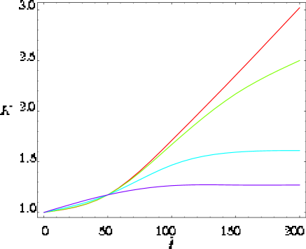
Figure 10.3: Schmidt number $K$ versus $\tilde{t}$ for $\tilde{\Gamma}=0$, $0.005$, $0.015$ and $0.03$. The higher curves correspond to the thinner $\Gamma$’s.

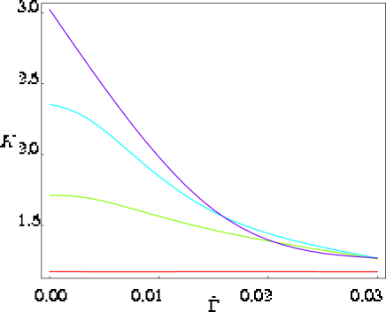
Figure 10.4: Schmidt number $K$ versus $\tilde{\Gamma}$ for $\tilde{t}=50$, $100$, $150$ and $200$. The higher curves correspond to the longer $t$’s.

10.3 Remarks

For the sake of completeness we point out that the term (10.16) may be important when $\Gamma$ is not so small, and there is a time in which this term becomes larger than the $\exp(-\tilde{\Gamma}\tilde{t})$ term. This value of $\tilde{t}$ is

$$\tilde{t}_{0}\simeq\frac{1}{\tilde{\Gamma}}\log\left[\frac{8\sqrt{2\pi}}{\tilde{\Gamma}}\frac{\tilde{E_{e}}^{5/2}(\tilde{E_{g}}+\tilde{E_{\gamma}})}{\sqrt{(\tilde{E_{e}}-\tilde{E_{g}}-\tilde{E_{\gamma}})^{2}+\tilde{\Gamma}^{2}/4}}\right].$$ (10.26)

The value of $\tilde{\Gamma}$ for which the term (10.16) becomes larger than the other terms ($\exp(-\tilde{\Gamma}\tilde{t})$ term and Lorentzian term) for the case here considered of $\tilde{m}_{g}=0.7$, $\tilde{m}_{\gamma}=0.1$ and for $\tilde{t}=50$ is around $\tilde{\Gamma}=1$, i.e., of $m_{e}$ order, which does not seem to be a realistic value in principle. However, some recent results [JMS⁺05] point to the possibility of decay in S-wave in such a way that the width is larger than the difference in energies between excited and ground states. In such a case, the contribution from $I_{cut}$ would be relevant.

In summary, we analyzed the generation of momentum entanglement in the decay of unstable systems described by a decay width $\Gamma$. We verify that, as expected, the entanglement grows with time until reaching an asymptotic maximum. On the other hand, unexpectedly, the wider the decay width $\Gamma$, the lesser the asymptotic attainable entanglement. We explain this apparently surprising result in terms of the fact that for wider width the mean life is shorter, so that the system evolves faster (during a shorter period) and can reach lesser entanglement than with longer mean lives.

Chapter 11 Maximum entanglement: The Dirac delta

One interesting (non-normalizable) amplitude when studying continuous variable entanglement is the Dirac delta. In this chapter we give [LL05a] a concise description of its entanglement content based on the method we proposed in Chapter 8 for computing the Schmidt decomposition of an amplitude with continuous variables.

In this case we have (see Chapter 8) $f(p,q)=\delta(p-q)$ and we take the same interval $(a,b)$ for $p$ and $q$ to apply our method, for analyzing its entanglement. We consider complete sets of orthonormal functions satisfying $O^{(1)}_{n}(k)=O^{(2)*}_{n}(k)$. A particular case is when they are real functions, as for example the typical orthogonal polynomials (Legendre, Hermite, Laguerre, Chebyshev,…) are. We must take into account that the Dirac delta is not a function but a distribution, and indeed is outside $L^{2}$. However, we can calculate the $C_{mn}$ and study how much entanglement does this state have. We obtain straightforwardly $C_{mn}=\delta_{mn}$. This gives

$$\delta(p-q)=\sum_{n=0}^{\infty}O^{(\alpha)*}_{n}(p)O^{(\alpha)}_{n}(q),$$ (11.1)

which is just the resolution of the identity as given in (8.4). The Schmidt decomposition of the Dirac delta is not unique, because all the weights $\sqrt{\lambda_{n}}$ are equal to one (they are degenerate). In fact, the decomposition can be done with any complete, denumerable set of orthonormal functions, in the form (8.4). This expression can be seen as an infinite entanglement case, in the sense explained below. The fact that all the weights are equal to one, makes sense only because we are considering a distribution, not an $L^{2}$ state. The sum of the squares of the weights, which must be equal to the square of the norm of the function $f(p,q)$, diverges because the Dirac delta is not square-integrable.

A possible measure of the entanglement of a state $f(p,q)$ in its Schmidt decomposition (A.14) is given by the von Neumann entropy [NC00]

$$S=-\sum_{n=0}^{\infty}\lambda_{n}\log_{2}\lambda_{n}.$$ (11.2)

This is usually called the entropy of entanglement.

The state of $L^{2}$ closer to (11.1) is the case of an entangled state with $N$ diagonal terms with equal $\lambda_{n}$, when $N$ goes to infinity. To be correctly normalized it verifies $\lambda_{n}=1/N$, $n=0,...,N-1$ and

$$S=-\lim_{N\rightarrow\infty}\sum_{n=0}^{N-1}\frac{1}{N}\log_{2}\frac{1}{N}=-\lim_{N\rightarrow\infty}\log_{2}\frac{1}{N}=\infty.$$ (11.3)

This is the maximum entanglement case. This provides an estimate of the entropy of the Dirac delta (were it in $L^{2}$). Another well-known way of obtaining the amount of entanglement of the Dirac delta is considering it as the limit of infinite squeezing of a bipartite Gaussian state [Gie01]. However, to our knowledge, the Schmidt decomposition of the Dirac delta has never been obtained before. We believe ours is an elegant result, that may clarify the entanglement structure of this distribution.

Part III Multipartite entanglement

Chapter 12 Sequential quantum cloning

12.1 Quantum cloning sequentially implemented

Multipartite entangled states stand up as the most versatile and powerful tool to perform information-processing protocols in quantum information science [BD00]. They arise as an invaluable resource in tasks such as quantum computation [DE98, RB01], quantum state teleportation [BEA00], quantum communication [ABH⁺01] and dense coding [BW92]. As a result, the controllable generation of these states becomes a crucial issue in the quest for quantum-informational proposals. However, the generation of multipartite entangled states through single global unitary operations is, in general, an extremely difficult experimental task. In this sense, the sequential generation studied by Schön et al. [SSV⁺05, SHW⁺06], where at each step one qubit is allowed to interact with an ancilla, appears as the most promising avenue. The essence of this sequential scheme is the successive interaction of each qubit initialized in the standard state $|0\rangle$ with an ancilla of a suitable dimension $D$ to generate the desired multiqubit state. In the last step, the qubit-ancilla interaction is chosen so as to decouple the final multiqubit entangled state from the auxiliary $D$-dimensional system, yielding [SSV⁺05]

$$|\Psi\rangle=\sum_{i_{1}\cdots i_{n}=0,1}\langle\varphi_{F}|V_{[n]}^{i_{n}}\cdots V_{[1]}^{i_{1}}|\varphi_{I}\rangle|i_{1}\cdots i_{n}\rangle,$$ (12.1)

where the $V_{[k]}^{i_{k}}$ are $D-$dimensional matrices arising from the isometries $V_{[k]}:{\cal{H}}_{A}\otimes\{|0\rangle\}\to{\cal{H}}_{A}\otimes{\cal{H}}_{B_{k}}$, with ${\cal{H}}_{A}=\mathbb{C}^{D}$ and ${\cal{H}}_{B_{k}}=\mathbb{C}^{2}$ being the Hilbert spaces for the ancilla and the $k$th qubit, respectively, and where $|\varphi_{I}\rangle$ and $|\varphi_{F}\rangle$ denote the initial and final states of the ancilla, respectively. The state (12.1) is, indeed, a Matrix-Product State (MPS) (cf. [Eck05, PGVWC06] and multiple references therein), already present in spin chains [AKLT87], classical simulations of quantum entangled systems [Vid03] and density-matrix renormalization group techniques [VPC04]. Moreover, it was proven that any multiqubit MPS can be sequentially generated using the recipe of Ref. [SSV⁺05]. Notice that in this formalism, the mutual qubit-ancilla interaction in each step $k$ completely determines the matrices $V_{[k]}^{i_{k}}$, $i_{k}=0,1$, whereas we enjoy some freedom to build such an interaction from a known $V_{[k]}^{i_{k}}$. This freedom stems from the very fact that in the proposed scheme only the initial state $|0\rangle$ for each qubit will be relevant.

Here we consider [DLL⁺06] the possibility of implementing quantum cloning based on a sequential protocol with the help of an ancillary system. This problem is certainly far from being an application of Ref. [SSV⁺05], given that the initial and final states are unknown. In this sense, any proposed strategy will be closer to the open problem of which global unitary operations (certainly not all of them) can be implemented through a sequential procedure. Despite the fundamental no-cloning theorem [WZ82, Die82], stating the impossibility to exactly clone an unknown quantum state, there exist several cloning techniques with a given optimal fidelity [SIGA05] (see Appendix B). These procedures differ either from the initial set of states to be cloned or from symmetry considerations. In general, an optimality condition of the cloning procedure is obtained via the maximization of the fidelity between the original qubit and each final clone state. We will show how to perform sequentially both the universal symmetric [BH96, GM97] and the economical phase-covariant symmetric quantum cloning [DM03, BDM05] from one qubit to $M$ clones. In the first case, a global unitary evolution transforms any input state $|\psi\rangle$ in a set of $M$ clones whose individual reduced states $\rho_{out}$ carry maximal fidelity with respect to $|\psi\rangle$: $F_{1,M}=\frac{2M+1}{3M}$. This cloning procedure is fully described by the evolution

$$|\psi\rangle\otimes|B\rangle\to\sum_{j=0}^{M-1}\alpha_{j}|(M-j)\psi,j\psi^{\perp}\rangle_{S}\otimes|(M-j-1)\psi^{*},j\psi^{*\perp}\rangle_{S},$$ (12.2)

where $|B\rangle$ denotes the initial blank state, $\alpha_{j}=\sqrt{\frac{2(M-j)}{M(M+1)}}$ and $|(M-j)\phi,j\phi^{\perp}\rangle_{S}$ denotes the normalized completely symmetric state with $(M-j)$ qubits in state $\phi$ and $j$ qubits in state $\phi^{\perp}$. As a relevant feature it must be noticed that the presence of $M-1$ additional so-called anticlones is necessary in order to perform this cloning procedure with the optimal fidelity. The anticlone state $\psi^{*}$ refers to the fact that they transform under rotations as the complex conjugate representation. For concreteness sake we have chosen $|\psi^{*}\rangle=\cos\theta/2|1\rangle+e^{-i\phi}\sin\theta/2|0\rangle$ in coincidence with the seminal paper by Bužek and Hillery [BH96], where $|\psi\rangle=\cos\theta/2|0\rangle+e^{i\phi}\sin\theta/2|1\rangle$. In the second case, motivated by quantum cryptoanalysis, the goal is to clone only those states belonging to the equatorial plane of the Bloch sphere, i.e. those such that $\theta=\pi/2$. Furthermore, we have only focused upon the cases where no anticlones are needed (hence the term economical). Under this assumption, imposing the purity of the joint state, the number of clones $M$ must be odd [DM03]. The cloning evolution is now given by

$$|\psi\rangle\otimes|B\rangle\to\frac{1}{\sqrt{2}}\left[|(k+1)0,k1\rangle_{S}+e^{i\phi}|k0,(k+1)1\rangle_{S}\right],$$ (12.3)

where $k=(M-1)/2$ and where we have followed the same convention as above. In order to employ the sequential ancilla-qubit device as a quantum cloning machine we will firstly elucidate the minimal dimension required for the ancilla. The basic idea is to express the final states (12.2) and (12.3) in its MPS form, following Vidal’s recipe [Vid03] (see Appendix C):

$$|\Phi\rangle=\sum_{i_{1}\dots i_{n}}\left(\sum_{\alpha_{1}\dots\alpha_{n-1}}\Gamma[1]^{i_{1}}_{\alpha_{1}}\lambda[1]_{\alpha_{1}}\Gamma[2]^{i_{2}}_{\alpha_{1}\alpha_{2}}\lambda[2]_{\alpha_{2}}\Gamma[3]^{i_{3}}_{\alpha_{2}\alpha_{3}}\dots\Gamma[n]_{\alpha_{n-1}}^{i_{n}}\right)|i_{1}\dots i_{n}\rangle.$$ (12.4)

We identify the matrices $V^{i_{k}}_{[k]}$ by matching indices in expressions (12.1) and (12.4). The indices $\alpha_{j}$ run from $1$ to $\chi$, where $\chi=\max_{\mathcal{P}}\{\chi_{\mathcal{P}}\}$, $\chi_{\mathcal{P}}$ denoting the rank of the reduced density matrix $\rho_{\mathcal{P}}$ for the bipartite partition $\mathcal{P}$ of the composite system [Vid03]. To clone an arbitrary input qubit state $|\psi\rangle=\alpha|0\rangle+\beta|1\rangle$, we exploit linearity and determine the minimal dimension $D_{i}$ of the ancilla to perform the cloning for the state $|0\rangle$ and then similarly for the state $|1\rangle$. Then we combine both results in a single ancilla to obtain its desired minimal dimension $D$. Let us focus upon the symmetric universal cloning of $|0\rangle$. To determine the minimal dimension $D_{0}$ of the ancilla we need to compute $\chi$, which can be undertaken without the exact MPS expression for the state. We need some previous results:

Proposition 1.

Let $|\psi\rangle$ and $|\phi\rangle$ be multipartite states of the same system related through an invertible local operator $F_{\mathcal{P}}=F_{A}\otimes F_{B}$ for the partition $\mathcal{P}=A|B$:

$$|\psi\rangle=F_{\mathcal{P}}|\phi\rangle.$$ (12.5)

Then $\chi_{\mathcal{P}}(\phi)=\chi_{\mathcal{P}}(\psi)$.

Proof.

Recalling that the rank of $\rho_{\mathcal{P}}$ coincides with the rank of the coefficient matrix $C_{\mathcal{P}}$ of the corresponding state for that partition $\mathcal{P}$, the application of the invertible local operator $F_{\mathcal{P}}$ amounts to changing the local basis of each part $A$ and $B$ in which the coefficient matrix is expressed. Since the rank is invariant under local changes of basis, we will have $\mathop{\rm r}\nolimits\left(C_{\mathcal{P}}(\phi)\right)=\mathop{\rm r}\nolimits\left(C_{\mathcal{P}}(\psi)\right)$ for the bipartite partition $\mathcal{P}$. Hence $\chi_{\mathcal{P}}(\phi)=\chi_{\mathcal{P}}(\psi)$. ∎

Proposition 2.

Let $C_{M|M-1}$ be the coefficient matrix of the state (12.2) for the partition $M|M-1$. Then

$$\mathop{\rm r}\nolimits(C_{M|M-1})=M.$$ (12.6)

Proof.

In virtue of the preceding proposition and using the invertible local operator $\mathcal{S}_{M}\otimes\mathcal{S}_{M-1}$, where $\mathcal{S}_{K}$ denotes the normalized symmetrizing operator for $K$ qubits, we only need to compute the rank of the coefficient matrix of

$$\sum_{j=0}^{M-1}\alpha_{j}|(M-j)0,j1\rangle\otimes|(M-j-1)1,j0\rangle,$$ (12.7)

where the states are no longer completely symmetrized. Given the orthonormality of the involved states and the number of different components ($M$), it is clear that there are only $M$ different rows, whereas the rest are all null, i.e. $\mathop{\rm r}\nolimits(C_{M|M-1})=M$. ∎

Finally we prove the following

Proposition 3.

Let $C_{k|2M-1-k}$ be the coefficient matrix of state (12.2) for the partition $k|2M-k-1$, where $k=1,2,\dots,2M-2$. Then

$$\mathop{\rm r}\nolimits(C_{k|2M-1-k})\leq\mathop{\rm r}\nolimits(C_{M|M-1})\qquad\forall k.$$ (12.8)

Proof.

The key point is to realize that the matrices $C_{k|2M-1-k}$ are obtained from $C_{M|M-1}$ by appropriately adjoining rows or columns to make them longer. From the preceding proof it is clear that there are only $M$ different rows in $C_{M|M-1}$, the rest being all null, thus the reordering procedure to build the other matrices cannot increase the former rank. Hence the stated result. ∎

With all these propositions it elementarily follows that $\chi=M$, i.e. that the minimal dimension $D_{0}$ to clone the $|0\rangle$ state is $D_{0}=M$, namely the number of clones to produce. Repeating the same argument for the initial state $|1\rangle$ we also conclude that the minimal dimension of the ancilla to clone the $|1\rangle$ state is $D_{1}=M$, as expected. Now we must combine both results to find $D$ for an arbitrary unknown state $|\psi\rangle=\alpha|0\rangle+\beta|1\rangle$. It is a wrong guessing to think that it should also be $D=M$ and, consequently, a different scheme must be given. The MPS expression of (12.2) for the original state $|0\rangle$ determines the $D$-dimensional matrices $V_{0[k]}^{i_{k}}$, whereas the corresponding MPS expression for the original state $|1\rangle$ determines $V_{1[k]}^{i_{k}}$,

$$|GM_{M}(0)\rangle=\sum_{i_{1}\dots i_{n}=0,1}\langle\varphi_{F}^{(0)}|V_{0[n]}^{i_{n}}\dots V_{0[1]}^{i_{1}}|0\rangle_{D}|i_{1}\dots i_{n}\rangle,$$

$$|GM_{M}(1)\rangle=\sum_{i_{1}\dots i_{n}=0,1}\langle\varphi_{F}^{(1)}|V_{1[n]}^{i_{n}}\dots V_{1[1]}^{i_{1}}|0\rangle_{D}|i_{1}\dots i_{n}\rangle.$$

Here, $|\varphi_{F}^{(0)}\rangle$ and $|\varphi_{F}^{(1)}\rangle$ can be calculated explicitly and will play an important role below.

We propose now to double the dimension of the ancilla, $\mathbb{C}^{D}\to\mathbb{C}^{2}\otimes\mathbb{C}^{D}$, in order to implement a deterministic protocol of sequential quantum cloning.

Protocol 1.

Let $V_{[k]}^{i_{k}}=|0\rangle\langle 0|\otimes V_{0[k]}^{i_{k}}+|1\rangle\langle 1|\otimes V_{1[k]}^{i_{k}}$. Then

1. Encode the unknown state $|\psi\rangle$ in the initial ancilla state $|\varphi_{I}\rangle=|\psi\rangle\otimes|0\rangle_{D}$.

2. Allow each qubit $k$ to interact with the ancilla according to the preceding $2D$-dimensional matrices $V_{[k]}^{i_{k}}$.

3. Perform a generalized Hadamard transformation upon the ancilla:

   $$|0\rangle\otimes|\varphi_{F}^{(0)}\rangle\to\frac{1}{\sqrt{2}}\left[|0\rangle\otimes|\varphi_{F}^{(0)}\rangle+|1\rangle\otimes|\varphi_{F}^{(1)}\rangle\right]$$ (12.10a)

   $$|1\rangle\otimes|\varphi_{F}^{(1)}\rangle\to\frac{1}{\sqrt{2}}\left[|0\rangle\otimes|\varphi_{F}^{(0)}\rangle-|1\rangle\otimes|\varphi_{F}^{(1)}\rangle\right]$$

   Note that the choice $\mathbb{C}^{D}\to\mathbb{C}^{2}\otimes\mathbb{C}^{D}$ (based on pedagogical reasons) could be changed, equivalently, to $\mathbb{C}^{D}\to\mathbb{C}^{2D}$. In this way, Eq. (12.10a) would not display entangled states but simple linear superpositions.

4. Perform a measurement upon the ancilla in the local basis $\{|0\rangle\otimes|\varphi_{F}^{(0)}\rangle,|1\rangle\otimes|\varphi_{F}^{(1)}\rangle\}$.

5. If the result is $|0\rangle\otimes|\varphi_{F}^{(0)}\rangle$ (which happens with probability $1/2$), the qubits are already in the desired state; if the result is $|1\rangle\otimes|\varphi_{F}^{(1)}\rangle$ (probability $1/2$), perform a local $\varphi=\pi$ phase gate upon each qubit, then they will end up in the desired state.

Proof.

After the first two steps, the joint state of the ancilla and the qubits is $\alpha\left(|0\rangle\otimes|\varphi_{F}^{(0)}\rangle\right)\otimes|GM_{M}(0)\rangle+\beta\left(|1\rangle\otimes|\varphi_{F}^{(1)}\rangle\right)|GM_{M}(1)\rangle$, where originally $|\psi\rangle=\alpha|0\rangle+\beta|1\rangle$. After the Hadamard rotation (step iii), this state becomes

$$\frac{1}{\sqrt{2}}\left(|0\rangle\otimes|\varphi_{F}^{(0)}\rangle\right)\otimes\left[\alpha|GM_{M}(0)\rangle+\beta|GM_{M}(1)\rangle\right]+$$

$$+\frac{1}{\sqrt{2}}\left(|1\rangle\otimes|\varphi_{F}^{(1)}\rangle\right)\otimes\left[\alpha|GM_{M}(0)\rangle-\beta|GM_{M}(1)\rangle\right]$$

The remaining steps follow immediately from this expresion and from linearity [GM97].

∎

Notice that despite the measurement process in step (iv), the final desired state is obtained with probability $1$. In summary, the minimal dimension $D$ of the ancilla for cloning $M$ qubits is $D=2\times M$, i.e. it grows linearly with the number of clones even although the dimension of their space grows exponentially ($2^{M}$). The reader can straightforwardly convince himself that were we to clone a $d$-dimensional system, the minimal dimension for the ancilla would be $D=d\times M$, with an obvious generalization of the preceding argument. For the symmetric phase-covariant cloning, the same arguments can be reproduced provided we realize that the first term of the r.h.s. of Eq. (12.3) can adopt a similar form to (12.2):

$$|(k+1)0,k1\rangle_{S}=\sum_{j=0}^{k}\gamma_{j}|(k+1-j)0,j1\rangle_{S}\otimes|(k-j)1,j0\rangle_{S},$$ (12.11)

where $\gamma_{j}\neq 0$ for all $j$, and similarly for the second term. Thus for symmetric phase-covariant cloning the minimal dimension for the ancilla is $D=2\times(k+1)=2\times\frac{M+1}{2}=M+1$. We see that the dimension of the ancilla $D$ also grows linearly with the number of clones, although it is now lesser than above. This is a direct consequence of reducing the set of possible original states to clone.

12.2 A specific illustrative case: $1\rightarrow 3$

In this section we explicitly compute the isometries for the universal symmetric quantum cloning from 1 qubit to 3 clones. We will show how the dimension of the ancilla is indeed $2\times 3=6$. We will be mainly using the formalism for computing the MPS form of an arbitrary multipartite state by Vidal [Vid03]. The final state after the cloning procedure for the $|\!\!\uparrow\rangle$, according to Gisin and Massar [GM97] is

$$|\Psi\rangle=\alpha_{0}|\!\!\uparrow\uparrow\uparrow\rangle|\!\!\downarrow\downarrow\rangle+\alpha_{1}\frac{|\!\!\uparrow\uparrow\downarrow\rangle+|\!\!\uparrow\downarrow\uparrow\rangle+|\!\!\downarrow\uparrow\uparrow\rangle}{\sqrt{3}}\frac{|\!\!\uparrow\downarrow\rangle+|\!\!\downarrow\uparrow\rangle}{\sqrt{2}}+\alpha_{2}\frac{|\!\!\uparrow\downarrow\downarrow\rangle+|\!\!\downarrow\uparrow\downarrow\rangle+|\!\!\downarrow\downarrow\uparrow\rangle}{\sqrt{3}}|\!\!\uparrow\uparrow\rangle$$ (12.12)

We now compute the Schmidt decomposition for the entangled state (12.12) in the partition $1|2345$:

$$|\Psi\rangle = \sqrt{N_{\uparrow}}|\!\!\uparrow\rangle\left[\underbrace{\frac{\alpha_{0}}{\sqrt{N_{\uparrow}}}|\!\!\uparrow\uparrow\downarrow\downarrow\rangle+\frac{\alpha_{1}}{\sqrt{3N_{\uparrow}}}\frac{(|\!\!\uparrow\downarrow\rangle+|\!\!\downarrow\uparrow\rangle)(|\!\!\uparrow\downarrow\rangle+|\!\!\downarrow\uparrow\rangle)}{\sqrt{2}}+\frac{\alpha_{2}}{\sqrt{3N_{\uparrow}}}|\!\!\downarrow\downarrow\uparrow\uparrow\rangle}\right]$$

$$\;\;\;\;\;\;\;\;\;\;\;\;\;\;\;\;\;\;\;\;\;\;\;\;\;\;\;\;\;\;\;\;\;\;\;\;\;\;\;\;\;\;\;\;\;\;\;\;\;\;\;\;\;\;\;\;\;\;\;\Phi^{[2...5]}_{\uparrow}$$

$$+\sqrt{N_{\downarrow}}|\!\!\downarrow\rangle\left[\underbrace{\frac{\alpha_{1}}{\sqrt{3N_{\downarrow}}}|\!\!\uparrow\uparrow\rangle\frac{|\!\!\uparrow\downarrow\rangle+|\!\!\downarrow\uparrow\rangle}{\sqrt{2}}+\frac{\alpha_{2}}{\sqrt{3N_{\downarrow}}}(|\!\!\uparrow\downarrow\rangle+|\!\!\downarrow\uparrow\rangle)|\!\!\uparrow\uparrow\rangle}\right],$$

$$\;\;\;\;\;\;\;\;\;\;\;\;\;\;\;\;\;\;\;\;\;\;\;\;\;\;\;\;\;\;\;\;\;\;\;\;\;\;\;\;\;\;\;\;\;\;\;\;\;\Phi^{[2...5]}_{\downarrow}$$

where $\Phi^{[2...5]}_{\uparrow}$ and $\Phi^{[2...5]}_{\downarrow}$ are the Schmidt vectors of the subsystem corresponding to qubits 2 to 5, and $N_{\uparrow}$, $N_{\downarrow}$ are the Schmidt coefficients, given by $N_{\uparrow}:=\alpha_{0}^{2}+\frac{2\alpha_{1}^{2}}{3}+\frac{\alpha_{2}^{2}}{3}$, $N_{\downarrow}:=\frac{\alpha_{1}^{2}}{3}+\frac{2\alpha_{2}^{2}}{3}$.

According to the protocol developed in [Vid03], we have, following its notation, (see Eq. (12.4) above)

$$[\lambda_{\alpha_{1}}^{[1]}]=(\sqrt{N_{\uparrow}},\sqrt{N_{\downarrow}})$$ (12.14)

$$[\Gamma_{\alpha_{1}}^{[1]\uparrow}]=(1,0);\;\;[\Gamma_{\alpha_{1}}^{[1]\downarrow}]=(0,1).$$ (12.15)

We proceed now iteratively, computing the Schmidt decomposition for state (12.12) in the partition $12|345$. It easily follows

$$|\Psi\rangle=\sqrt{N_{\uparrow\uparrow}}|\!\!\uparrow\uparrow\rangle\left[\underbrace{\frac{\alpha_{0}}{\sqrt{N_{\uparrow\uparrow}}}|\!\!\uparrow\downarrow\downarrow\rangle+\frac{\alpha_{1}}{\sqrt{3N_{\uparrow\uparrow}}}|\!\!\downarrow\rangle\frac{|\!\!\uparrow\downarrow\rangle+|\!\!\downarrow\uparrow\rangle}{\sqrt{2}}}\right]+$$

$$\;\;\;\;\;\;\;\;\;\;\;\;\;\;\;\;\;\;\;\;\;\;\;\;\;\;\;\;\;\;\;\;\;\;\;\;\;\;\;\;\;\;\;\;\;\;\;\;\;\;\Phi^{[3...5]}_{\uparrow\uparrow}$$

$$+\sqrt{2N_{\uparrow\downarrow+\downarrow\uparrow}}\frac{|\!\!\uparrow\downarrow\rangle+|\!\!\downarrow\uparrow\rangle}{\sqrt{2}}\left[\underbrace{\frac{\alpha_{1}}{\sqrt{3N_{\uparrow\downarrow+\downarrow\uparrow}}}|\!\!\uparrow\rangle\frac{|\!\!\uparrow\downarrow\rangle+|\!\!\downarrow\uparrow\rangle}{\sqrt{2}}+\frac{\alpha_{2}}{\sqrt{3N_{\uparrow\downarrow+\downarrow\uparrow}}}|\!\!\downarrow\uparrow\uparrow\rangle}\right]$$

$$\;\;\;\;\;\;\;\;\;\;\;\;\;\;\;\;\;\;\;\;\;\;\;\;\;\;\;\;\;\;\;\;\;\;\;\;\;\;\;\;\;\;\;\;\;\;\;\;\;\;\;\;\;\;\;\;\;\;\;\;\;\;\;\;\;\;\Phi^{[3...5]}_{\uparrow\downarrow+\downarrow\uparrow}$$

$$+\sqrt{N_{\downarrow\downarrow}}|\!\!\downarrow\downarrow\rangle\underbrace{\frac{\alpha_{2}}{\sqrt{3N_{\downarrow\downarrow}}}|\!\!\uparrow\uparrow\uparrow\rangle},$$ (12.16)

$$\;\;\;\;\;\;\;\;\;\;\;\;\;\;\;\;\;\;\;\;\;\;\Phi^{[3...5]}_{\downarrow\downarrow}$$

where $\Phi^{[3...5]}_{\uparrow\uparrow}$, $\Phi^{[3...5]}_{\uparrow\downarrow+\downarrow\uparrow}$ and $\Phi^{[3...5]}_{\downarrow\downarrow}$ are the Schmidt vectors of the subsystem corresponding to qubits 3 to 5, and $N_{\uparrow\uparrow}$, $2N_{\uparrow\downarrow+\downarrow\uparrow}$ and $N_{\downarrow\downarrow}$ are the Schmidt coefficients, given by $N_{\uparrow\uparrow}:=\alpha_{0}^{2}+\frac{\alpha_{1}^{2}}{3}$, $2N_{\uparrow\downarrow+\downarrow\uparrow}:=\frac{2\alpha_{1}^{2}}{3}+\frac{2\alpha_{2}^{2}}{3}$, $N_{\downarrow\downarrow}:=\frac{\alpha_{2}^{2}}{3}$.

According to [Vid03], we have in this case

$$[\lambda_{\alpha_{2}}^{[2]}]=(\sqrt{N_{\uparrow\uparrow}},\sqrt{2N_{\uparrow\downarrow+\downarrow\uparrow}},\sqrt{N_{\downarrow\downarrow}})$$ (12.17)

$$[\Gamma_{\alpha_{1}\alpha_{2}}^{[2]\uparrow}]=\left(\begin{array}[]{ccc}\frac{1}{\sqrt{N_{\uparrow}}}&0&0\\ 0&\frac{1}{\sqrt{2N_{\downarrow}}}&0\end{array}\right)$$ (12.20)

$$[\Gamma_{\alpha_{1}\alpha_{2}}^{[2]\downarrow}]=\left(\begin{array}[]{ccc}0&\frac{1}{\sqrt{2N_{\uparrow}}}&0\\ 0&0&\frac{1}{\sqrt{N_{\downarrow}}}\end{array}\right).$$ (12.23)

We proceed now with the partition $123|45$ of the state $|\Psi\rangle$. Eq. (12.12) is indeed the Schmidt decomposition for this partition, where the Schmidt vectors of the subsystem associated to qubits 4 and 5 are $\Phi_{\uparrow\uparrow\uparrow}^{[4,5]}:=|\!\!\downarrow\downarrow\rangle$, $\Phi_{(\uparrow\uparrow\downarrow)}^{[4,5]}:=\frac{|\!\uparrow\downarrow\rangle+|\!\downarrow\uparrow\rangle}{\sqrt{2}}$, and $\Phi_{(\uparrow\downarrow\downarrow)}^{[4,5]}:=|\!\!\uparrow\uparrow\rangle$.

With the notation $(...)$ we denote here the combination maximally symmetrized.

Following [Vid03], we have

$$[\lambda_{\alpha_{3}}^{[3]}]=(\alpha_{0},\alpha_{1},\alpha_{2})$$ (12.24)

$$[\Gamma_{\alpha_{2}\alpha_{3}}^{[3]\uparrow}]=\left(\begin{array}[]{ccc}\frac{1}{\sqrt{N_{\uparrow\uparrow}}}&0&0\\ 0&\frac{1}{\sqrt{3N_{\uparrow\downarrow+\downarrow\uparrow}}}&0\\ 0&0&\frac{1}{\sqrt{3N_{\downarrow\downarrow}}}\end{array}\right)$$ (12.28)

$$[\Gamma_{\alpha_{2}\alpha_{3}}^{[3]\downarrow}]=\left(\begin{array}[]{ccc}0&\frac{1}{\sqrt{3N_{\uparrow\uparrow}}}&0\\ 0&0&\frac{1}{\sqrt{3N_{\uparrow\downarrow+\downarrow\uparrow}}}\\ 0&0&0\end{array}\right).$$ (12.32)

Finally we compute the Schmidt decomposition of $|\Psi\rangle$ in the remaining partition $1234|5$, which turns to be

$$|\Psi\rangle=\sqrt{N_{4:1,\downarrow}}\left[\frac{\alpha_{0}|\!\!\uparrow\uparrow\uparrow\rangle|\!\!\downarrow\rangle}{\sqrt{N_{4:1,\downarrow}}}+\frac{\alpha_{1}|(\uparrow\uparrow\downarrow)\rangle|\uparrow\rangle}{\sqrt{2N_{4:1,\downarrow}}}\right]|\!\!\downarrow\rangle$$

$$+\sqrt{N_{4:1,\uparrow}}\left[\frac{\alpha_{1}|(\uparrow\uparrow\downarrow)\rangle|\!\!\downarrow\rangle}{\sqrt{2N_{4:1,\uparrow}}}+\frac{\alpha_{2}|(\uparrow\downarrow\downarrow)\rangle|\!\!\uparrow\rangle}{\sqrt{N_{4:1,\uparrow}}}\right]|\!\!\uparrow\rangle,$$ (12.33)

where the Schmidt vectors associated to the subsystem of qubit 5 are $\Phi_{4:1,\downarrow}^{[5]}:=|\!\!\downarrow\rangle$ and $\Phi_{4:1,\uparrow}^{[5]}:=|\!\!\uparrow\rangle$, and the Schmidt coefficients are $N_{4:1,\downarrow}:=\alpha_{0}^{2}+\frac{\alpha_{1}^{2}}{2}$, $N_{4:1,\uparrow}:=\frac{\alpha_{1}^{2}}{2}+\alpha_{2}^{2}$.

In this case we have

$$[\lambda_{\alpha_{4}}^{[4]}]=(\sqrt{N_{4:1,\downarrow}},\sqrt{N_{4:1,\uparrow}})$$ (12.35)

$$[\Gamma_{\alpha_{3}\alpha_{4}}^{[4]\uparrow}]=\left(\begin{array}[]{cc}0&0\\ \frac{1}{\sqrt{2N_{4:1,\downarrow}}}&0\\ 0&\frac{1}{\sqrt{N_{4:1,\uparrow}}}\end{array}\right)$$ (12.39)

$$[\Gamma_{\alpha_{3}\alpha_{4}}^{[4]\downarrow}]=\left(\begin{array}[]{cc}\frac{1}{\sqrt{N_{4:1,\downarrow}}}&0\\ 0&\frac{1}{\sqrt{2N_{4:1,\uparrow}}}\\ 0&0\end{array}\right).$$ (12.43)

Finally we have the remaining matrices $[\Gamma_{\alpha_{4}}^{[5]\uparrow}]$ and $[\Gamma_{\alpha_{4}}^{[5]\downarrow}]$,

$$[\Gamma_{\alpha_{4}}^{[5]\uparrow}]=\left(\begin{array}[]{c}0\\ 1\end{array}\right);\;\;[\Gamma_{\alpha_{4}}^{[5]\downarrow}]=\left(\begin{array}[]{c}1\\ 0\end{array}\right).$$ (12.48)

The last step left is to match the $\lambda^{\prime}s$ and $\Gamma^{\prime}s$ with the $V^{\prime}s$ (isometries) of Eq. (12.1). An easy comparison between Eqs. (12.1) and (12.4) yields

$$[V_{0[1]}^{\uparrow}]_{ij}:=\left(\begin{array}[]{ccc}\sqrt{N_{\uparrow}}&0&0\\ 0&\frac{1}{\sqrt{2}}&0\\ 0&0&\frac{1}{\sqrt{2}}\end{array}\right);\;\;[V_{0[1]}^{\downarrow}]_{ij}:=\left(\begin{array}[]{ccc}0&\frac{1}{\sqrt{2}}&0\\ \sqrt{N_{\downarrow}}&0&0\\ 0&0&\frac{1}{\sqrt{2}}\end{array}\right)$$ (12.55)

$$[V_{0[2]}^{\uparrow}]_{ij}:=\left(\begin{array}[]{ccc}\sqrt{\frac{N_{\uparrow\uparrow}}{N_{\uparrow}}}&0&0\\ 0&\sqrt{\frac{N_{\uparrow\downarrow+\downarrow\uparrow}}{N_{\downarrow}}}&0\\ 0&0&\frac{1}{\sqrt{2}}\end{array}\right);\;\;[V_{0[2]}^{\downarrow}]_{ij}:=\left(\begin{array}[]{ccc}0&0&\frac{1}{\sqrt{2}}\\ \sqrt{\frac{N_{\uparrow\downarrow+\downarrow\uparrow}}{N_{\uparrow}}}&0&0\\ 0&\sqrt{\frac{N_{\downarrow\downarrow}}{N_{\downarrow}}}&0\end{array}\right)$$ (12.62)

$$[V_{0[3]}^{\uparrow}]_{ij}:=\left(\begin{array}[]{ccc}\frac{\alpha_{0}}{\sqrt{N_{\uparrow\uparrow}}}&0&0\\ 0&\frac{\alpha_{1}}{\sqrt{3N_{\uparrow\downarrow+\downarrow\uparrow}}}&0\\ 0&0&\frac{\alpha_{2}}{\sqrt{3N_{\downarrow\downarrow}}}\end{array}\right);\;\;[V_{0[3]}^{\downarrow}]_{ij}:=\left(\begin{array}[]{ccc}0&0&0\\ \frac{\alpha_{1}}{\sqrt{3N_{\uparrow\uparrow}}}&0&0\\ 0&\frac{\alpha_{2}}{\sqrt{3N_{\uparrow\downarrow+\downarrow\uparrow}}}&0\end{array}\right)$$ (12.69)

$$[V_{0[4]}^{\uparrow}]_{ij}:=\left(\begin{array}[]{ccc}0&\frac{1}{\sqrt{2}}&0\\ 0&0&1\\ 0&0&0\end{array}\right);\;\;[V_{0[4]}^{\downarrow}]_{ij}:=\left(\begin{array}[]{ccc}1&0&0\\ 0&\frac{1}{\sqrt{2}}&0\\ 0&0&0\end{array}\right)$$ (12.76)

$$[V_{0[5]}^{\uparrow}]_{ij}:=\left(\begin{array}[]{ccc}0&1&0\\ 0&0&0\\ 0&0&\frac{1}{\sqrt{2}}\end{array}\right);\;\;[V_{0[5]}^{\downarrow}]_{ij}:=\left(\begin{array}[]{ccc}1&0&0\\ 0&0&0\\ 0&0&\frac{1}{\sqrt{2}}\end{array}\right)$$ (12.83)

The interested reader may straightforwardly check the isometry condition $V_{0[k]}^{\uparrow{\dagger}}V_{0[k]}^{\uparrow}+V_{0[k]}^{\downarrow{\dagger}}V_{0[k]}^{\downarrow}=I_{3\times 3}$, $k=1,...,5$ that the matrices verify, as expected. Some remarks are to be pointed out:

• The dimension of the ancilla Hilbert space is in this case $D_{0}=3$ (the matrices $V$ explicitly calculated have dimension 3$\times$3), in concordance with the results of the previous section: the dimension $D_{0}$ equals the number of clones $M$ for the universal symmetric cloning (3, in this particular example). The global dimension for this case, $D$, is, according to our protocol stated in previous section, $D=2\times D_{0}=6$.

• Notice the change of order between the matrices $V$ and Vidal’s matrices $\Gamma$ and $\lambda$: we have expressed the $V$ matrices in order to be applied from right to left, sequentially, upon the initial state $|\varphi_{I}\rangle:=(1,0,0)^{T}$. The matrices 1 to 3 create the three clones in a highly entangled state with the ancilla, and the remaining matrices 4 and 5 uncouple the clones from the ancilla by creating the two anticlones. The final state of the ancilla after successive application of the five matrices $V_{0[i]}$ results $|\varphi_{F}\rangle:=(1,0,0)$, as the interested reader may readily check.

• The previous matrices are the corresponding to the sequential generation of state (12.12), which is the cloning of state $|\!\!\uparrow\rangle$. In order to clone an arbitrary superposition $\alpha|\!\!\uparrow\rangle+\beta|\!\!\downarrow\rangle$, according to our protocol, the sequential generation of the cloning of state $|\!\!\downarrow\rangle$ is needed. This state is obtained from state (12.12) by doing the substitution $0\leftrightarrow 1$. Accordingly, the matrices $V_{1[k]}^{i_{k}}$ are obtained from the ones (12.83) by $V_{1[k]}^{i_{k}}=V_{0[k]}^{\bar{i}_{k}}$, where $\bar{i}:=i\oplus 1$. The global unitary operations are 6$\times$6 matrices built from $V_{0[k]}$ and $V_{1[k]}$ by diagonal blocks, according to our protocol 1.

12.3 Isometries in the general case $1\rightarrow M$

For the symmetric universal cloning $1\rightarrow M$ we now give in detail the $2D-$dimensional matrices $V_{[k]}^{i_{k}}$ driving us to a concrete sequential scheme. The procedure for the calculation in this case follows the same lines of the previous example, although here the method relies in a highly symbolic notation based on maximally symmetrized states.

To explicitly obtain the isometries, we firstly compute the Schmidt decomposition (see Appendix A) for the multipartite state $|(M-j)\uparrow j\downarrow\rangle_{S}$, where here $|k\uparrow k^{\prime}\downarrow\rangle_{S}$ denotes the maximally-symmetrized state with $k$ qubits $\uparrow$ and $k^{\prime}$ qubits $\downarrow$. We will be interested in the Schmidt decomposition for the $1|2...M$ bipartition, that gives

$$|(M-j)\uparrow j\downarrow\rangle_{S}=\sqrt{\frac{M-j}{M}}|\!\!\uparrow\rangle|(M-j-1)\uparrow j\downarrow\rangle_{S}+\sqrt{\frac{j}{M}}|\!\!\downarrow\rangle|(M-j)\uparrow(j-1)\downarrow\rangle_{S}.$$

(12.84)

The coefficients $\sqrt{\frac{M-j}{M}}$ and $\sqrt{\frac{j}{M}}$ follow directly from straightforward combinatorics.

Expression (12.84) will be the basis for our computation of the isometries.

We consider now the general state with $M$ clones and $M-1$ anticlones for the initial qubit $\uparrow$ [GM97]

$$|\!\!\uparrow\rangle\to|\psi\rangle=\sum_{j=0}^{M-1}\alpha_{j}|(M-j)\uparrow,j\downarrow\rangle_{S}\otimes|(M-j-1)\downarrow,j\uparrow\rangle_{S},$$ (12.85)

where the first vector in the explicitly indicated tensor product corresponds to the clones and the second one to the anticlones, and $\alpha_{j}=\sqrt{\frac{2(M-j)}{M(M+1)}}$.

The Schmidt decomposition of (12.85) for the $1|2...2M-1$ bipartition, is, according to (12.84)

$$|\psi\rangle=|\!\!\uparrow\rangle\left[\alpha_{0}|(M-1)\uparrow\rangle_{S}|(M-1)\downarrow\rangle_{S}+\alpha_{1}\sqrt{\frac{M-1}{M}}|(M-2)\uparrow 1\downarrow\rangle_{S}|(M-2)\downarrow 1\uparrow\rangle_{S}+\right.$$

$$...+\left.\alpha_{M-1}\sqrt{\frac{1}{M}}|(M-1)\downarrow\rangle_{S}|(M-1)\uparrow\rangle_{S}\right]+|\!\!\downarrow\rangle\left[\alpha_{1}\sqrt{\frac{1}{M}}|(M-1)\uparrow\rangle_{S}|(M-2)\downarrow 1\uparrow\rangle_{S}\right.$$

$$+\alpha_{2}\sqrt{\frac{2}{M}}|(M-2)\uparrow 1\downarrow\rangle_{S}|(M-3)\downarrow 2\uparrow\rangle_{S}+...+\left.\alpha_{M-1}\sqrt{\frac{M-1}{M}}|1\uparrow(M-2)\downarrow\rangle_{S}\right.$$

$$\left.\frac{}{}\times|(M-1)\uparrow\rangle_{S}\right].$$ (12.86)

The (normalized) Schmidt vectors of the previous decomposition associated to the subspace of qubits $2...2M-1$ are directly read from it and are given by

$$\Phi_{\uparrow}^{[2...2M-1]}$$

$$:=\frac{1}{\sqrt{N_{\uparrow}}}\left[\alpha_{0}|(M-1)\uparrow\rangle_{S}|(M-1)\downarrow\rangle_{S}+\alpha_{1}\sqrt{\frac{M-1}{M}}|(M-2)\uparrow 1\downarrow\rangle_{S}\right.$$

$$\times|(M-2)\downarrow 1\uparrow\rangle_{S}+...+\left.\alpha_{M-1}\sqrt{\frac{1}{M}}|(M-1)\downarrow\rangle_{S}|(M-1)\uparrow\rangle_{S}\right],$$ (12.87)

$$\Phi_{\downarrow}^{[2...2M-1]}$$

$$:=\frac{1}{\sqrt{N_{\downarrow}}}\left[\alpha_{1}\sqrt{\frac{1}{M}}|(M-1)\uparrow\rangle_{S}|(M-2)\downarrow 1\uparrow\rangle_{S}\right.+\alpha_{2}\sqrt{\frac{2}{M}}|(M-2)\uparrow 1\downarrow\rangle_{S}$$

$$\times|(M-3)\downarrow 2\uparrow\rangle_{S}+...+\left.\alpha_{M-1}\sqrt{\frac{M-1}{M}}|1\uparrow(M-2)\downarrow\rangle_{S}|(M-1)\uparrow\rangle_{S}\right],$$ (12.88)

where $N_{\uparrow}:=\alpha_{0}^{2}+\alpha_{1}^{2}(M-1)/M+\alpha_{2}^{2}(M-2)/M+...$, and $N_{\downarrow}:=\alpha_{1}^{2}/M+2\alpha_{2}^{2}/M+...$.

According to the protocol developed in [Vid03], we have, following its notation, (see Eq. (12.4) above)

$$[\lambda_{\alpha_{1}}^{[1]}]=(\sqrt{N_{\uparrow}},\sqrt{N_{\downarrow}})$$ (12.89)

$$[\Gamma_{\alpha_{1}}^{[1]\uparrow}]=(1,0);\;\;[\Gamma_{\alpha_{1}}^{[1]\downarrow}]=(0,1).$$ (12.90)

We now proceed iteratively, just as in the $1\rightarrow 3$ case shown above. We compute the Schmidt decomposition for every bipartition, $12...k|k+1...2M-1$, $k=2,...,2M-2$, extract the Schmidt coefficients, $\lambda^{[k]}$, and the Schmidt vectors, $\Phi^{[k+1...2M-1]}$, and, applying Vidal’s recipe, we obtain the $\Gamma^{[k]i_{k}}$ matrices. We made the calculation along this lines, by splitting it in 3 steps: the partitions with $k=1,...,M-1$, that create the clones. The partition with $k=M$, that attains the multiqubit state of the clones with highest entanglement with the ancilla of all the sequential protocol, and the remaining partitions with $k=M+1,...,2M-2$, that create the anticlones. The need for this splitting of the computation is due to the different role of clones and anticlones: they are not mutually symmetric. The result of our computation is

$$1\leq n\leq M-1\rightarrow$$

$$\Gamma^{[n]\uparrow}\lambda^{[n]}=\left(\begin{array}[]{ccccc}\sqrt{\frac{N_{n\uparrow}}{N_{(n-1)\uparrow}}}&0&\ldots&0&0\\ 0&\sqrt{\frac{N_{(n-1)\uparrow 1\downarrow}}{N_{(n-2)\uparrow 1\downarrow}}}&\ldots&0&0\\ \vdots&&\ddots&&\vdots\\ 0&0&\ldots&\sqrt{\frac{N_{1\uparrow(n-1)\downarrow}}{N_{(n-1)\downarrow}}}&0\end{array}\right)_{n\times n+1},$$ (12.95)

$$\Gamma^{[n]\downarrow}\lambda^{[n]}=\left(\begin{array}[]{ccccc}0&\sqrt{\frac{N_{(n-1)\uparrow 1\downarrow}}{N_{(n-1)\uparrow}}}&0&\ldots&0\\ 0&0&\sqrt{\frac{N_{(n-2)\uparrow 2\downarrow}}{N_{(n-2)\uparrow 1\downarrow}}}&\ldots&0\\ \vdots&&&\ddots&\vdots\\ 0&0&0&\ldots&\sqrt{\frac{N_{n\downarrow}}{N_{(n-1)\downarrow}}}\end{array}\right)_{n\times n+1},$$ (12.100)

$$n=M\rightarrow$$

$$\Gamma^{[M]\uparrow}\lambda^{[M]}=\left(\begin{array}[]{cccccc}\frac{\alpha_{0}}{\sqrt{N_{(M-1)\uparrow}}}&0&\ldots&\dots&\ldots&0\\ 0&\frac{\alpha_{1}/\sqrt{M}}{\sqrt{N_{(M-2)\uparrow 1\downarrow}}}&\ldots&\ldots&\ldots&0\\ \vdots&\vdots&\ddots&&&\vdots\\ \vdots&\vdots&&\frac{\alpha_{k}/\sqrt{\binom{M}{k}}}{\sqrt{N_{(M-k-1)\uparrow k\downarrow}}}&&\vdots\\ \vdots&\vdots&&&\ddots&0\\ 0&0&\ldots&\ldots&0&\frac{\alpha_{M-1}/\sqrt{M}}{\sqrt{N_{(M-1)\downarrow}}}\end{array}\right)_{M\times M},$$ (12.107)

$$\Gamma^{[M]\downarrow}\lambda^{[M]}=\left(\begin{array}[]{cccccc}0&\frac{\alpha_{1}/\sqrt{M}}{\sqrt{N_{(M-1)\uparrow}}}&0&\ldots&\ldots&0\\ \vdots&0&\ddots&&&\vdots\\ \vdots&\vdots&&\frac{\alpha_{k}/\sqrt{\binom{M}{k}}}{\sqrt{N_{(M-k)\uparrow(k-1)\downarrow}}}&&\vdots\\ \vdots&\vdots&&&\ddots&0\\ \vdots&0&\ldots&\ldots&0&\frac{\alpha_{M-1}/\sqrt{M}}{\sqrt{N_{1\uparrow(M-2)\downarrow}}}\\ 0&\ldots&\ldots&\ldots&\ldots&0\end{array}\right)_{M\times M},$$ (12.114)

$$0\leq j\leq M-2\rightarrow$$

$$\Gamma^{[M+1+j]\uparrow}\lambda^{[M+1+j]}=\left(\begin{array}[]{ccccc}0&0&\ldots&\ldots&0\\ \sqrt{\frac{1}{M-1-j}}&0&\ldots&\ldots&0\\ 0&\ddots&&&\vdots\\ \vdots&&\sqrt{\frac{k}{M-1-j}}&&\vdots\\ \vdots&&&\ddots&0\\ 0&\ldots&\ldots&0&1\end{array}\right)_{M-j\times M-j-1},$$ (12.121)

$$\Gamma^{[M+1+j]\downarrow}\lambda^{[M+1+j]}=\left(\begin{array}[]{cccccc}1&0&\ldots&\ldots&0\\ 0&\ddots&&&\vdots\\ \vdots&&\sqrt{\frac{M-j-k}{M-1-j}}&&\vdots\\ \vdots&&&\ddots&0\\ 0&\ldots&\ldots&0&\sqrt{\frac{1}{M-1-j}}\\ 0&\ldots&\ldots&\ldots&0\end{array}\right)_{M-j\times M-j-1},$$ (12.128)

where the coefficients $N_{k\uparrow k^{\prime}\downarrow}$ are the normalization coefficients of the corresponding Schmidt vectors as outlined for the $1\rightarrow 3$ case in this chapter, and previously in this section. They are given by

$$N_{i\uparrow j\downarrow}:=\frac{1}{\binom{i+j}{i}}\sum_{k=j}^{M-1}|\alpha_{k}|^{2}\frac{\binom{M-k}{i}\binom{k}{j}}{\binom{M}{i+j}}.$$ (12.129)

The corresponding isometries $V_{[k]}$ for the universal symmetric cloning $1\rightarrow M$ of qubits, built upon the $\Gamma$ matrices and $\lambda$ vectors, according to our protocol, are given in Table 12.1.

The matrices $V_{[k]}^{i_{k}}$ coincide also with the ones for the symmetric phase-covariant cloning just by doing the substitutions $M\rightarrow\frac{M+1}{2}$ and $\alpha_{j}\rightarrow\gamma_{j}:=\sqrt{\frac{\binom{k+1}{k+1-j}\binom{k}{j}}{\binom{2k+1}{k+1}}}$.

	$k=0$	$k=1$
$\left[V_{0[1]}^{k}\right]_{ij}=$	$\left\{\begin{array}[]{cc}\delta_{ij}\mathcal{C}(2-i,i-1)&1\leq i,j\leq 2\\ \frac{1}{\sqrt{2}}\delta_{ij}&\textrm{otherwise}\end{array}\right.$	$\left\{\begin{array}[]{cc}\delta_{i,3-j}\mathcal{C}(2-i,i-1)&1\leq i,j\leq 2\\ \frac{1}{\sqrt{2}}\delta_{ij}&\textrm{otherwise}\end{array}\right.$
$\left[V_{0[n]}^{k}\right]_{ij}=$	$\left\{\begin{array}[]{cc}\delta_{ij}\frac{\mathcal{C}(n+1-i,i-1)}{\mathcal{C}(n-i,i-1)}&1\leq i,j\leq n\\ \frac{1}{\sqrt{2}}\delta_{ij}&\textrm{otherwise}\end{array}\right.$	$\left\{\begin{array}[]{cc}\frac{1}{\sqrt{2}}&i=1,j=n+1\\ \delta_{i,j+1}\frac{\mathcal{C}(n-j,j)}{\mathcal{C}(n-j,j-1)}&2\leq i\leq n+1;1\leq j\leq n\\ \frac{1}{\sqrt{2}}\delta_{ij}&\textrm{otherwise}\end{array}\right.$
$\left[V_{0[M]}^{k}\right]_{ij}=$	$\left\{\begin{array}[]{cc}\delta_{ij}\frac{\alpha_{i-1}}{\mathcal{C}(M-i,i-1)\sqrt{\binom{M}{i-1}}}&1\leq i,j\leq M\end{array}\right.$	$\left\{\begin{array}[]{cc}\delta_{i,j+1}\frac{\alpha_{j}}{\mathcal{C}(M-j,j-1)\sqrt{\binom{M}{j}}}&1\leq i,j\leq M\\ \end{array}\right.$
$\left[V_{0[M+n]}^{k}\right]_{ij}=$	$\left\{\begin{array}[]{cc}\delta_{i,j-1}\sqrt{\frac{i}{M-n}}&1\leq i\leq M-n;2\leq j\leq M-n+1\\ 0&i=M-n+1;1\leq j\leq M\\ \frac{1}{\sqrt{2}}\delta_{ij}&\textrm{otherwise}\end{array}\right.$	$\left\{\begin{array}[]{cc}\delta_{ij}\sqrt{\frac{M-n+1-i}{M-n}}&1\leq i,j\leq M-n\\ 0&i=M-n+1;1\leq j\leq M\\ \frac{1}{\sqrt{2}}\delta_{ij}&\textrm{otherwise}\end{array}\right.$

Table 12.1: Explicit form of the isometries for universal symmetric quantum cloning $1\rightarrow M$.

Here $\mathcal{C}(i,j):=\sqrt{N_{i\uparrow j\downarrow}}=\sqrt{\frac{1}{\binom{i+j}{i}}\sum_{k=j}^{M-1}|\alpha_{k}|^{2}\frac{\binom{M-k}{i}\binom{k}{j}}{\binom{M}{i+j}}}$ (we use the convention $\binom{p}{q}=0$ if $q>p$) and $1<n\leq M-1$. Complementarily, we also have $V_{1[k]}^{i_{k}}=V_{0[k]}^{\bar{i_{k}}}$, where by $\bar{i}$ we indicate $\bar{i}:=i\oplus 1$. The reader can readily check that the minimal dimension for the ancilla is $2\times M$. When sequentially applying these matrices to the initial state $|\varphi_{I}\rangle$ of the ancilla, one can check, as expected, that if we were to stop at the $M$th step, the $M$ clones would have already been produced with the desired properties, although in a highly entangled state with the ancilla. To arrive at a final uncoupled state, the remaining $M-1$ anticlones must be operated upon by the ancilla.

In conclusion, following the idea that some (certainly not all) unitary operations upon a multiqubit state can be implemented sequentially by successive interactions between each qubit and an ancilla, we have shown how to reproduce both the symmetric universal and symmetric phase-covariant cloning operations. For the universal cloning we have proved that the minimal dimension for the ancilla must be $D=2M$, where $M$ denotes the number of clones, thus showing a linear dependence. The original state must be encoded in a $D-$dimensional state. For the phase-covariant case, the dimension $D$ of the ancilla can be reduced to $D=M+1$, even lower. In both cases, the ancilla ends up uncoupled to the qubits. Along similar lines, this sequential cloning protocol can be adapted to other proposals, such as asymmetric universal quantum cloning or other state-dependent cloning. This procedure can have notable experimental interest, since it provides a systematic method to furnish any multiqubit state using only sequential two-body (qubit-ancilla) operations.

Chapter 13 Inductive classification of multipartite entanglement under stochastic local operations and classical communication

A comprehensive understanding of entanglement is still lacking, mainly because it is a highly counterintuitive feature of quantum systems (non-separability [Bel87]) and because its analysis can be undertaken under different, although complementary, standpoints. As prominent examples the subjects of deciding in full generality whether a given state carries entanglement or not and how much entanglement the system should be attributed to are vivid open questions (cf. e.g. [Bru02] and references therein). This state of affairs is critical in multipartite systems, where most applications find their desired utility.

Among others, part of the efforts are being dedicated to classify under diversely motivated criteria the types of entanglement which a multipartite system can show. It is in this sense desirable, independently of these criteria, to have classification methods valid for any number $N$ of entangled systems. One of these most celebrated criteria to carry out such a classification was provided in [DVC00]. In physical terms Dür et al. defined an entanglement class as the set of pure states which can be interrelated through stochastic local operations and classical communications (SLOCC hereafter) or equivalently, as those pure states which can carry out the same quantum-informational tasks with non-null possibly different probabilities. They also proved the mathematical counterpart of this characterization: two states $\Psi$ and $\bar{\Psi}$ of a given system belong to the same entanglement class if, and only if, there exist invertible local operators (ILO’s hereafter; that is, nonsingular matrices), which we agree on denoting as $F^{[i]}$ such that $\bar{\Psi}=F^{[1]}\otimes\dots\otimes F^{[N]}(\Psi)$. Moreover, they provided the first classification under this criterion of tripartite multiqubit entanglement, giving birth to the two well-known genuine entanglement triqubit classes named as $GHZ$ and $W$ classes. Later on, exploiting some accidental facts in group theory, Verstraete et al. [VDMV02] gave rise to the classification of $4$-qubit states.

Regretfully none of the previous works allowed one to succeed in obtaining a generalizable method. In the second case, the exploitation of a singular fact such as the isomorphism $SU(2)\otimes SU(2)\simeq SO(4)$ is clearly useless in a general setting; in the first case, the use of quantitative entanglement measures specifically designed for three qubits, as the $3-$tangle [CKW00], to discern among different entanglement classes discourages one to follow up the same trend, since we would have to be able to build more generic entanglement measures, per se a formidable task. However, Verstraete et al. [VDM03] succeeded in this approach by introducing the so-called normal forms, namely those pure states such that all reduced local operators are proportional to the identity matrix. These authors also provided a systematic, mostly numerical, constructive procedure to find the ILO’s bringing an arbitrary pure state to a normal form. Furthermore, the use of these normal forms allowed them to introduce entanglement measures (entanglement monotones [Vid00], indeed), which offered the possibility to quantify the amount of entanglement in the original state. For completeness’ sake let us recall that classification under SLOCC is coarser than that using only local unitaries, that is in which every $F^{[k]}$ is unitary. Nevertheless relevant results in this realm can be found in the literature [GRB98, AAC⁺00, CHS00, GAFW06].

Here we offer [LLSS06] an alternative and complementary approach to the classification under SLOCC based on an analysis of the singular value decomposition (SVD) of the coefficient matrix of the pure state in an arbitrary product basis. The coefficient matrix is chosen according to the partition $1|2\dots N$ with the subsequent goal of establishing a recursive procedure allowing one to elucidating the entanglement classes under SLOCC provided such a classification is known with one less qubit. The key feature in this scheme is the structure of the right singular subspace, i.e. of the subspace generated by the right singular vectors of the coefficient matrix, set up according to the entanglement classes which its generators belong to. As a secondary long-term goal, the approach seeks possible connections to the matrix product state (MPS) formalism (cf. [Eck05, PGVWC06] and multiple references therein), which is becoming increasingly ubiquitous in different fields such as spin chains [AKLT87], classical simulations of quantum entangled systems [Vid03], density-matrix renormalization group techniques [VPC04] and sequential generation of entangled multiqubit states [SSV⁺05, SHW⁺06].

This chapter uses a more mathematical notation. The canonical orthonormal basis in $\mathbb{C}^{N}$ will be denoted by $\{e_{j}\}_{j=1,\dots,N}$ (correspondingly in physics the kets $|j-1\rangle$). Normalization is not relevant in elucidating the entanglement class which a state belongs to. Thus we will deal with unnormalized vectors and non-unit-determinant ILO’s. In the SVD of an arbitrary matrix (cf. appendix), $V$ and $W$ will denote the left and right unitary matrix, whereas $\Sigma$ will stand for the diagonal possibly rectangular matrix with the singular values as entries. In the multiqubit cases, we will agree on denoting by small Greek letters $\phi,\varphi,...$ vectors belonging to $\mathbb{C}^{2}$, whereas capital Greek letters $\Psi,\Phi,...$ will denote a generic entangled state in $\mathbb{C}^{2}\otimes\mathbb{C}^{2}$.

The chapter is organized as follows. In section 13.1 the entanglement of two qubits is revisited with a reformulation of the Schmidt decomposition criterion in terms of the singular subspaces. In section 13.2 the extension to the three-qubit case is developed in detail and the principles of the generalization to multipartite and arbitrary-dimension systems are discussed in section 13.3. Some concluding remarks close the chapter.

13.1 Bipartite entanglement

13.1.1 The Schmidt decomposition criterion revisited

The determination of entanglement of pure states of bipartite systems in any dimensions, in general, and in two dimensions (qubits), in particular, was solved long ago with the aid of the well-known Schmidt decomposition [Sch06, EK95] (see Appendix A), by which any bipartite state can be written as a biorthogonal combination

$$\Psi=\sum_{n=1}^{\min(N_{1},N_{2})}\sqrt{\lambda_{n}}\phi_{n}^{(1)}\otimes\psi_{n}^{(2)},$$ (13.1)

where $\lambda_{1}\geq\lambda_{2}\geq\dots\geq 0$ for all $n$ and $N_{i}$ denotes the dimension of subsystem $i$. If $\lambda_{n}=0$ except for only one index $\lambda_{1}\neq 0$, then the state is a product state; on the contrary, if $\lambda_{n}\neq 0$ for two or more indices, then the state is an entangled state. Furthermore, $\lambda_{n}$ coincides with the common eigenvalues of both reduced density operators. Thus, to practically determine the entangled or separable character of a given pure state all we must do is to compute the spectrum of $\rho_{1}$ or $\rho_{2}$ or equivalently to analyze the dimensionality of their ranges. This is the backbone in the study of $3-$partite entanglement carried out in [DVC00].

Followingly in order to pave the way for a generalization to multipartite systems, we will reformulate the Schmidt decomposition criterion for bipartite systems focusing upon the subspace generated by the singular vectors. We need the next

Definition 5.

We will denote by $\mathfrak{V}$ (resp. $\mathfrak{W}$) the subspace generated by the left (resp. right) singular vectors, i.e. $\mathfrak{V}=\mathop{\rm span}\nolimits\{v_{1},\dots,v_{k}\}$ (resp. $\mathfrak{W}=\mathop{\rm span}\nolimits\{w_{1},\dots,w_{k}\}$).

We can now state the following

Theorem 1.

Let $\Psi\in\mathbb{C}^{m}\otimes\mathbb{C}^{n}$ and $C(\Psi)$ denote the matrix of coefficients of $\Psi$ in an arbitrary common product basis. Then $\Psi$ is a product state if and only if $\dim\mathfrak{W}=1$ (or alternatively $\dim\mathfrak{V}=1$).

Proof.

Let $\{e_{i}\}_{i=1,\dots,m}$ and $\{f_{j}\}_{j=1,\dots,n}$ denote bases in $\mathbb{C}^{m}$ and $\mathbb{C}^{n}$, respectively. Then any vector $\Psi\in\mathbb{C}^{m}\otimes\mathbb{C}^{n}$ can be written as

$$\Psi=\sum_{i=1}^{m}\sum_{j=1}^{n}c_{ij}e_{i}\otimes f_{j},$$ (13.2)

where $c_{ij}$ are the complex coeficients of $\Psi$, which we arrange as:

$$C(\Psi)\equiv\begin{pmatrix}c_{11}&\dots&c_{1n}\\ \vdots&\ddots&\vdots\\ c_{m1}&\dots&c_{mn}\end{pmatrix}.$$ (13.3)

The matrix $C(\Psi)\equiv C$ always admits a SVD, given by $C=V\Sigma W^{\dagger}$, where $V$ and $W$ are unitary matrices and $\Sigma$ is a diagonal matrix with entries $\sigma_{k}$ (the singular values, indeed). Thus

$$c_{ij}=\sum_{k=1}^{\min(m,n)}v_{ik}\sigma_{k}w_{jk}^{*}.$$ (13.4)

Inserting (13.4) into (13.2) and identifying new bases $\{\bar{e}_{i}\}_{i=1,2}$ and $\{\bar{f}_{j}\}_{j=1,2}$ we arrive at the well known Schmidt decomposition

$$\Psi=\sum_{k=1}^{\min(m,n)}\sigma_{k}\bar{e}_{k}\otimes\bar{f}_{k}.$$ (13.5)

The number of non-null singular values coincides with the rank of $\Sigma$, which in turn coincides with the dimensions of $\mathfrak{V}$ and $\mathfrak{W}$.

∎

From the proof we can deduce a practical method to recognize where a bipartite system is entangled or not:

Corollary 1.

Let $\Psi\in\mathbb{C}^{m}\otimes\mathbb{C}^{n}$ denote the state of a bipartite quantum system and $C(\Psi)$ its coefficient matrix in an arbitrary product basis. Then $\Psi$ is a product state if, and only if, $\mathop{\rm r}\nolimits(C(\Psi))=1$.

13.1.2 Classification of two-qubit entanglement under SLOCC

We only need one further tool to find the classification of bipartite entanglement under SLOCC, which is established as follows:

Proposition 4.

Let $\Psi,\bar{\Psi}\in\mathbb{C}^{2}\otimes\mathbb{C}^{2}$ denote two two-qubit states related by SLOCC, i.e.

$$\bar{\Psi}=F^{[1]}\otimes F^{[2]}(\Psi),$$ (13.6)

where $F^{[1]}$ and $F^{[2]}$ are non-singular operators upon $\mathbb{C}^{2}$. Then their corresponding coefficient matrices $C,\bar{C}$ in an arbitrary product basis are related through

$$\bar{C}=(F^{[1]^{T}}V)\Sigma(F^{[2]\dagger}W)^{\dagger}.$$ (13.7)

Proof.

Just substitute $\Psi=\sum_{i,j=1,2}c_{ij}e_{i}\otimes f_{j}$ in (13.6) and identify indices. ∎

The key idea in our analysis is to recognize the effect of the ILO’s $F^{[i]}$ upon the singular vectors. If $v_{j}$ (resp. $w_{j}$) is a left (resp. right) singular vector for the matrix coefficient $C$, then $F^{[1]T}(v_{j})$ (resp. $F^{[2]\dagger}(w_{j})$) is a left (resp. right) “singular vector” for the new matrix coefficient $\bar{C}$. In order to ease the notation, we will agree hereafter on relating $\Psi$ and $\bar{\Psi}$ through $\bar{\Psi}=F^{[1]T}\otimes F^{[2]\dagger}(\Psi)$, which allows us to drop the transpose and Hermitian conjugation in future considerations.

The case of two qubits is elementary, since there is no much space to discuss. The bases in which the coefficient matrix will be expressed are the canonical orthonormal basis $\{e_{1},e_{2}\}$ in $\mathbb{C}^{2}$. Only two options are present: either $\dim\mathfrak{W}=1$ or $\dim\mathfrak{W}=2$. In the first case, after choosing $F^{[1]}$ such that

$$F^{[1]}(v_{1}) = \frac{1}{\sigma_{1}}e_{1},$$ (13.8a)

$$F^{[2]}(w_{1}) = e_{1},$$ (13.8b)

the new coefficient matrix will turn into $\bar{C}=\left(\begin{smallmatrix}1&0\\ 0&0\end{smallmatrix}\right)$, which corresponds to the product state $\bar{\Psi}=e_{1}\otimes e_{1}$. We will agree on stating that $\Psi$ belongs to the entanglement class denoted by $00$.

In the second case, where $\sigma_{1}\geq\sigma_{2}>0$, after choosing $F^{[1]}$ and $F^{[2]}$ such that

$$F^{[1]}(v_{1})=\frac{1}{\sigma_{1}}e_{1}, F^{[1]}(v_{2})=\frac{1}{\sigma_{2}}e_{2},$$ (13.9a)

$$F^{[2]}(w_{1})=e_{1}, F^{[2]}(w_{2})=e_{2},$$ (13.9b)

the new coefficient matrix will be $\bar{C}=\left(\begin{smallmatrix}1&0\\ 0&1\end{smallmatrix}\right)$, which corresponds to the entangled state $\bar{\Psi}=e_{1}\otimes e_{1}+e_{2}\otimes e_{2}$. Now we say that $\Psi$ belongs to the class $\Psi^{+}$.

The reader can readily check by simple inspection how in the first case the canonical matrix $\bar{C}$ has rank one, whereas in the second it has rank $2$, as expected. In summary, only two classes are possible, namely $00$ and $\Psi^{+}$.

13.2 Tripartite entanglement

The classification of tripartite pure states is performed along the same lines, namely choosing the ILO’s $F^{[i]}$ so that the final coefficient matrix reduces to a canonical one. In order to find such canonical matrices, we must be exhaustive in the considerations of all possibilities when discussing about $\mathfrak{V}$ and $\mathfrak{W}$.

The analysis of tripartite entanglement can be undertaken upon three possible coefficient matrices, arising from the three different ways to group the indices, that is, since $\Psi=\sum_{i_{1},i_{2},i_{3}=1,2}c_{i_{1}i_{2}i_{3}}e_{i_{1}}\otimes e_{i_{2}}\otimes e_{i_{3}}$, where as before $\{e_{k}\}$ denotes the canonical orthonormal basis in $\mathbb{C}^{2}$, we have

$$C^{(1)}\equiv C_{1|23} = \begin{pmatrix}c_{111}&c_{112}&c_{121}&c_{122}\\ c_{211}&c_{212}&c_{221}&c_{222}\end{pmatrix},$$ (13.10a)

$$C^{(2)}\equiv C_{2|13} = \begin{pmatrix}c_{111}&c_{112}&c_{211}&c_{212}\\ c_{121}&c_{122}&c_{221}&c_{222}\end{pmatrix},$$ (13.10b)

$$C^{(3)}\equiv C_{3|12} = \begin{pmatrix}c_{111}&c_{121}&c_{211}&c_{221}\\ c_{112}&c_{122}&c_{212}&c_{222}\end{pmatrix}.$$ (13.10c)

There is no loss of generality in choosing one of them, since the analysis will be exhaustive. Hereafter we will choose $C=C^{(1)}$. Notice that now the left singular vectors of $C$ belong to $\mathbb{C}^{2}$ whereas the right singular vectors are in $\mathbb{C}^{2}\otimes\mathbb{C}^{2}$. Also, we immediately realize that only two possibles options arise, namely $\dim\mathfrak{W}=1$ or $\dim\mathfrak{W}=2$, since there are at most two positive singular values. The recursivity appears when classifying the different structures which the subspace $\mathfrak{W}$ can show. The classification of these subspaces is performed according to the entanglement classes which their generators belong to. In order to do that we need the following result, which was firstly proved in the context of entanglement theory in [STV98]. We offer an alternative proof in order to illustrate our methods.

Proposition 5.

Any two-dimensional subspace in $\mathbb{C}^{2}\otimes\mathbb{C}^{2}$ contains at least one product vector.

Proof.

Let $V$ be a two-dimensional subspace of $\mathbb{C}^{2}\otimes\mathbb{C}^{2}$. With no loss of generality two entangled vectors can be chosen as generators of $V$ with coefficient matrices given by $C_{1}=\mathbb{I}$ and $C_{2}$ being an arbitrary rank-2 matrix in the product canonical basis. Then it is always possible to find non-null complex numbers $\alpha$ and $\beta$ such that $\alpha\mathbb{I}+\beta C_{2}$ has rank one. ∎

In other words, this proposition shows that $\mathop{\rm span}\nolimits\{\Psi_{1},\Psi_{2}\}$ always equals either $\mathop{\rm span}\nolimits\{\phi_{1}\otimes\psi_{1},\phi_{2}\otimes\psi_{2}\}$ or $\mathop{\rm span}\nolimits\{\phi\otimes\psi,\Psi\}$, where implicit are the assumptions that different indices denote linear independence and in the last case only one product unit vector can be found. Thus, with the same convention, the right singular subspace $\mathfrak{W}$ can show six different structures, namely $\mathop{\rm span}\nolimits\{\phi\otimes\psi\}$, $\mathop{\rm span}\nolimits\{\Psi\}$, $\mathop{\rm span}\nolimits\{\phi\otimes\psi_{1},\phi\otimes\psi_{2}\}$, $\mathop{\rm span}\nolimits\{\phi_{1}\otimes\psi,\phi_{2}\otimes\psi\}$, $\mathop{\rm span}\nolimits\{\phi_{1}\otimes\psi_{1},\phi_{2}\otimes\psi_{2}\}$ and $\mathop{\rm span}\nolimits\{\phi\otimes\psi,\Psi\}$. We can now state our result, already contained in [DVC00] with different criteria:

Theorem 2.

Let $\Psi\in\mathbb{C}^{2}\otimes\mathbb{C}^{2}\otimes\mathbb{C}^{2}$ be the pure state of a tripartite system. Then $\Psi$ can be reduced through SLOCC to one of the following six states, which corresponds to the six possible entanglement classes, according to the following table:

Class	Canonical vector	Canonical matrix	$\mathfrak{W}$
$000$	$e_{1}\otimes e_{1}\otimes e_{1}$	$\begin{pmatrix}1&0&0&0\\ 0&0&0&0\end{pmatrix}$	$\mathop{\rm span}\nolimits\{\phi\otimes\psi\}$
$0_{1}\Psi_{23}^{+}$	$e_{1}\otimes e_{1}\otimes e_{1}+e_{1}\otimes e_{2}\otimes e_{2}$	$\begin{pmatrix}1&0&0&1\\ 0&0&0&0\end{pmatrix}$	$\mathop{\rm span}\nolimits\{\Psi\}$
$0_{2}\Psi_{13}^{+}$	$e_{1}\otimes e_{1}\otimes e_{1}+e_{2}\otimes e_{1}\otimes e_{2}$	$\begin{pmatrix}1&0&0&0\\ 0&1&0&0\end{pmatrix}$	$\phi\otimes\mathbb{C}^{2}$
$0_{3}\Psi_{12}^{+}$	$e_{1}\otimes e_{1}\otimes e_{1}+e_{2}\otimes e_{2}\otimes e_{1}$	$\begin{pmatrix}1&0&0&0\\ 0&0&1&0\end{pmatrix}$	$\mathbb{C}^{2}\otimes\psi$
$GHZ$	$e_{1}\otimes e_{1}\otimes e_{1}+e_{2}\otimes e_{2}\otimes e_{2}$	$\begin{pmatrix}1&0&0&0\\ 0&0&0&1\end{pmatrix}$	$\mathop{\rm span}\nolimits\{\phi_{1}\otimes\psi_{1},\phi_{2}\otimes\psi_{2}\}$
$W$	$e_{1}\otimes e_{1}\otimes e_{2}+e_{1}\otimes e_{2}\otimes e_{1}+e_{2}\otimes e_{1}\otimes e_{1}$	$\begin{pmatrix}0&1&1&0\\ 1&0&0&0\end{pmatrix}$	$\mathop{\rm span}\nolimits\{\phi_{1}\otimes\psi_{1},\Psi\}$

Table 13.1: Genuine entanglement classes for three qubits

Proof.

We discuss depending on $\mathfrak{W}$:

1. $\mathfrak{W}=\mathop{\rm span}\nolimits\{\phi\otimes\psi\}$. In this case, $w_{1}=\phi\otimes\psi$. Choose the ILO’s $F^{[k]}$, $k=1,2,3$ so that

   $$F^{[1]}(v_{1}) = \frac{1}{\sigma_{1}}e_{1},$$ (13.11a)

   $$F^{[2]}(\phi) = e_{1},$$ (13.11b)

   $$F^{[3]}(\psi) = e_{1}.$$ (13.11c)

   Then the new coefficient matrix will be

   $$\bar{C} = \begin{pmatrix}\frac{1}{\sigma_{1}}&\cdot\\ 0&\cdot\end{pmatrix}\cdot\begin{pmatrix}\sigma_{1}&0&0&0\\ 0&0&0&0\end{pmatrix}\cdot\begin{pmatrix}1&0&0&0\\ \cdot&\cdot&\cdot&\cdot\\ \cdot&\cdot&\cdot&\cdot\\ \cdot&\cdot&\cdot&\cdot\end{pmatrix}=$$ (13.12)

   $$= \begin{pmatrix}1&0&0&0\\ 0&0&0&0\end{pmatrix},$$ (13.13)

   which corresponds to the state $e_{1}\otimes e_{1}\otimes e_{1}$, and where the dots $\cdot$ indicates the irrelevant character of that entry.

2. $\mathfrak{W}=\mathop{\rm span}\nolimits\{\Psi\}$. In this case $w_{1}=\phi_{1}\otimes\psi_{1}+\phi_{2}\otimes\psi_{2}$. Choose the ILO’s so that

   $$F^{[1]}(v_{1})=\frac{1}{\sigma_{1}}e_{1},$$ (13.14a)

   $$F^{[2]}(\phi_{1})=e_{1}, F^{[2]}(\phi_{2})=e_{2},$$ (13.14b)

   $$F^{[3]}(\psi_{1})=e_{1}, F^{[3]}(\psi_{2})=e_{2}.$$ (13.14c)

   Then the new coefficient matrix will be

   $$\bar{C} = \begin{pmatrix}\frac{1}{\sigma_{1}}&\cdot\\ 0&\cdot\end{pmatrix}\cdot\begin{pmatrix}\sigma_{1}&0&0&0\\ 0&0&0&0\end{pmatrix}\cdot\begin{pmatrix}1&0&0&1\\ \cdot&\cdot&\cdot&\cdot\\ \cdot&\cdot&\cdot&\cdot\\ \cdot&\cdot&\cdot&\cdot\end{pmatrix}=$$ (13.15)

   $$= \begin{pmatrix}1&0&0&1\\ 0&0&0&0\end{pmatrix},$$ (13.16)

   which corresponds to the state $e_{1}\otimes e_{1}\otimes e_{1}+e_{1}\otimes e_{2}\otimes e_{2}$.

3. $\mathfrak{W}=\phi\otimes\mathbb{C}^{2}=\mathop{\rm span}\nolimits\{\phi\otimes\psi_{1},\phi\otimes\psi_{2}\}$. In this case $w_{1}=\mu_{11}\phi\otimes\psi_{1}+\mu_{12}\phi\otimes\psi_{2}$ and $w_{2}=\mu_{21}\phi\otimes\psi_{1}+\mu_{22}\phi\otimes\psi_{2}$, where the matrix $[\mu_{ij}]$ has rank $2$, since $w_{1}$ and $w_{2}$ are linear independent (orthonormal, indeed). Choose the ILO’s so that

   $$F_{1}^{[1]}(v_{1})=\frac{1}{\sigma_{1}}e_{1},\qquad F_{1}^{[1]}(v_{2})=\frac{1}{\sigma_{2}}e_{2},$$ (13.17a)

   $$F^{[1]}_{2}=[F_{2}^{[1]}(e_{1})\ F_{2}^{[1]}(e_{2})]=[\mu_{ij}^{*}]^{-1},$$ (13.17b)

   $$F^{[1]}=F_{2}^{[1]}F_{1}^{[1]},$$ (13.17c)

   $$F^{[2]}(\phi)=e_{1},$$ (13.17d)

   $$F^{[3]}(\psi_{1})=e_{1},\qquad F^{[3]}(\psi_{2})=e_{2}.$$ (13.17e)

   Then the new coefficient matrix will be

   $$\bar{C} = \begin{pmatrix}\mu_{11}^{*}&\mu_{12}^{*}\\ \mu_{21}^{*}&\mu_{22}^{*}\end{pmatrix}^{-1}\cdot\begin{pmatrix}\frac{1}{\sigma_{1}}&0\\ 0&\frac{1}{\sigma_{2}}\end{pmatrix}\cdot\begin{pmatrix}\sigma_{1}&0&0&0\\ 0&\sigma_{2}&0&0\end{pmatrix}\cdot\begin{pmatrix}\mu_{11}^{*}&\mu_{12}^{*}&0&0\\ \mu_{21}^{*}&\mu_{22}^{*}&0&0\\ \cdot&\cdot&\cdot&\cdot\\ \cdot&\cdot&\cdot&\cdot\end{pmatrix}=$$ (13.18)

   $$= \begin{pmatrix}1&0&0&0\\ 0&1&0&0\end{pmatrix},$$

   which corresponds to the state $e_{1}\otimes e_{1}\otimes e_{1}+e_{2}\otimes e_{1}\otimes e_{2}$.

4. $\mathfrak{W}=\mathbb{C}^{2}\otimes\psi=\mathop{\rm span}\nolimits\{\phi_{1}\otimes\psi,\phi_{2}\otimes\psi\}$. In this case $w_{1}=\mu_{11}\phi_{1}\otimes\psi+\mu_{12}\phi_{2}\otimes\psi$ and $w_{2}=\mu_{21}\phi_{1}\otimes\psi+\mu_{22}\phi_{2}\otimes\psi$, where the matrix $[\mu_{ij}]$ has rank $2$, since $w_{1}$ and $w_{2}$ are linear independent (orthonormal, indeed). Choose the ILO’s so that

   $$F_{1}^{[1]}(v_{1})=\frac{1}{\sigma_{1}}e_{1},\qquad F_{1}^{[1]}(v_{2})=\frac{1}{\sigma_{2}}e_{2},$$ (13.19a)

   $$F^{[1]}_{2}=[F_{2}^{[1]}(e_{1})\ F_{2}^{[1]}(e_{2})]=[\mu_{ij}^{*}]^{-1},$$ (13.19b)

   $$F^{[1]}=F_{2}^{[1]}F_{1}^{[1]},$$ (13.19c)

   $$F^{[2]}(\phi_{1})=e_{1},\qquad F^{[2]}(\phi_{2})=e_{2},$$ (13.19d)

   $$F^{[3]}(\psi)=e_{1}.$$ (13.19e)

   Then the new coefficient matrix will be

   $$\bar{C} = \begin{pmatrix}\mu_{11}^{*}&\mu_{12}^{*}\\ \mu_{21}^{*}&\mu_{22}^{*}\end{pmatrix}^{-1}\cdot\begin{pmatrix}\frac{1}{\sigma_{1}}&0\\ 0&\frac{1}{\sigma_{2}}\end{pmatrix}\cdot\begin{pmatrix}\sigma_{1}&0&0&0\\ 0&\sigma_{2}&0&0\end{pmatrix}\cdot\begin{pmatrix}\mu_{11}^{*}&0&\mu_{12}^{*}&0\\ \mu_{21}^{*}&0&\mu_{22}^{*}&0\\ \cdot&\cdot&\cdot&\cdot\\ \cdot&\cdot&\cdot&\cdot\end{pmatrix}=$$ (13.20)

   $$= \begin{pmatrix}1&0&0&0\\ 0&0&1&0\end{pmatrix},$$

   which corresponds to the state $e_{1}\otimes e_{1}\otimes e_{1}+e_{2}\otimes e_{2}\otimes e_{1}$.

5. $\mathfrak{W}=\mathop{\rm span}\nolimits\{\phi_{1}\otimes\psi_{1},\phi_{2}\otimes\psi_{2}\}$. In this case $w_{1}=\mu_{11}\phi_{1}\otimes\psi_{1}+\mu_{12}\phi_{2}\otimes\psi_{2}$ and $w_{2}=\mu_{21}\phi_{1}\otimes\psi_{1}+\mu_{22}\phi_{2}\otimes\psi_{2}$, where the matrix $[\mu_{ij}]$ has rank $2$, since $w_{1}$ and $w_{2}$ are linear independent (orthonormal, indeed). Choose the ILO’s so that

   $$F_{1}^{[1]}(v_{1})=\frac{1}{\sigma_{1}}e_{1},\qquad F_{1}^{[1]}(v_{2})=\frac{1}{\sigma_{2}}e_{2},$$ (13.21a)

   $$F^{[1]}_{2}=[F_{2}^{[1]}(e_{1})\ F_{2}^{[1]}(e_{2})]=[\mu_{ij}^{*}]^{-1},$$ (13.21b)

   $$F^{[1]}=F_{2}^{[1]}F_{1}^{[1]},$$ (13.21c)

   $$F^{[2]}(\phi_{1})=e_{1},\qquad F^{[2]}(\phi_{2})=e_{2},$$ (13.21d)

   $$F^{[3]}(\psi_{1})=e_{1},\qquad F^{[3]}(\psi_{2})=e_{2}.$$ (13.21e)

   Then the new coefficient matrix will be

   $$\bar{C} = \begin{pmatrix}\mu_{11}^{*}&\mu_{12}^{*}\\ \mu_{21}^{*}&\mu_{22}^{*}\end{pmatrix}^{-1}\cdot\begin{pmatrix}\frac{1}{\sigma_{1}}&0\\ 0&\frac{1}{\sigma_{2}}\end{pmatrix}\cdot\begin{pmatrix}\sigma_{1}&0&0&0\\ 0&\sigma_{2}&0&0\end{pmatrix}\cdot\begin{pmatrix}\mu_{11}^{*}&0&0&\mu_{12}^{*}\\ \mu_{21}^{*}&0&0&\mu_{22}^{*}\\ \cdot&\cdot&\cdot&\cdot\\ \cdot&\cdot&\cdot&\cdot\end{pmatrix}=$$ (13.22)

   $$= \begin{pmatrix}1&0&0&0\\ 0&0&0&1\end{pmatrix},$$

   which corresponds to the state $e_{1}\otimes e_{1}\otimes e_{1}+e_{2}\otimes e_{2}\otimes e_{2}$.

6. $\mathfrak{W}=\mathop{\rm span}\nolimits\{\phi_{1}\otimes\psi_{1},\Psi\}$. In this notation, implicit is the assumption that only one product unit vector can be found in $\mathfrak{W}$. In this case $\Psi$ can be chosen so that $\Psi=\phi_{1}\otimes\psi_{2}+\phi_{2}\otimes\psi_{1}$. Thus the singular vectors can always be expressed as $w_{1}=\mu_{11}\left(\phi_{1}\otimes\psi_{2}+\phi_{2}\otimes\psi_{1}\right)+\mu_{12}\phi_{1}\otimes\psi_{1}$ and $w_{2}=\mu_{21}\left(\phi_{1}\otimes\psi_{2}+\phi_{2}\otimes\psi_{1}\right)+\mu_{22}\phi_{1}\otimes\psi_{1}$, where the matrix $[\mu_{ij}]$ has rank $2$, since $w_{1}$ and $w_{2}$ are linear independent (orthonormal, indeed). Choose the ILO’s so that

   $$F_{1}^{[1]}(v_{1})=\frac{1}{\sigma_{1}}e_{1},\qquad F_{1}^{[1]}(v_{2})=\frac{1}{\sigma_{2}}e_{2},$$ (13.23a)

   $$F^{[1]}_{2}=[F_{2}^{[1]}(e_{1})\ F_{2}^{[1]}(e_{2})]=[\mu_{ij}^{*}]^{-1},$$ (13.23b)

   $$F^{[1]}=F_{2}^{[1]}F_{1}^{[1]},$$ (13.23c)

   $$F^{[2]}(\phi_{1})=e_{1}\qquad F^{[2]}(\phi_{2})=e_{2},$$ (13.23d)

   $$F^{[3]}(\psi_{1})=e_{1}\qquad F^{[3]}(\psi_{2})=e_{2}.$$ (13.23e)

   Then the new coefficient matrix will be

   $$\bar{C} = \begin{pmatrix}\mu_{11}^{*}&\mu_{12}^{*}\\ \mu_{21}^{*}&\mu_{22}^{*}\end{pmatrix}^{-1}\cdot\begin{pmatrix}\frac{1}{\sigma_{1}}&0\\ 0&\frac{1}{\sigma_{2}}\end{pmatrix}\cdot\begin{pmatrix}\sigma_{1}&0&0&0\\ 0&\sigma_{2}&0&0\end{pmatrix}\cdot\begin{pmatrix}\mu_{12}^{*}&\mu_{11}^{*}&\mu_{11}^{*}&0\\ \mu_{22}^{*}&\mu_{21}^{*}&\mu_{21}^{*}&0\\ \cdot&\cdot&\cdot&\cdot\\ \cdot&\cdot&\cdot&\cdot\end{pmatrix}=$$ (13.24)

   $$= \begin{pmatrix}0&1&1&0\\ 1&0&0&0\end{pmatrix},$$

   which corresponds to the state $e_{1}\otimes e_{1}\otimes e_{2}+e_{1}\otimes e_{2}\otimes e_{1}+e_{2}\otimes e_{1}\otimes e_{1}$.

Since there is no more options for the subspace $\mathfrak{W}$ we have already considered all possible alternatives. ∎

In conclusion, we have found that there are six classes of entanglement, named after [DVC00] as $000$, $0_{i_{1}}\Psi^{+}_{i_{2}i_{3}}$, $GHZ$ and $W$. The theorem also indicates how to practically classify a given state $\Psi$: compute the SVD of its coefficient matrix and elucidate the structure of $\mathop{\rm span}\nolimits\{w_{1},w_{2}\}$. We include a further proposition comprising the practical implementation of this result. We need to introduce the following definition.

Definition 6.

Let $w_{j}=e_{1}\otimes w_{j1}+e_{2}\otimes w_{j2}\in\mathbb{C}^{2}\otimes\mathbb{C}^{2}$ be an arbitrary vector. We associate a two-dimensional matrix $W_{j}$ to $w_{j}$ by defining

$$W_{j}=[w_{j1}\ w_{j2}].$$ (13.25)

This definition will be mainly applied to the right singular vectors of the coefficient matrix $C$. As usual, the singular values of $C$ will be denoted by $\sigma_{k}$, in nonincreasing order, and $\sigma(A)$ denotes the spectrum of a matrix $A$. Our proposal to implement the preceding result is

Theorem 3.

Let $\Psi$ denote the pure state of a tripartite system and $C^{(i)}$ its coefficient matrix according to the partitions $i|jk$ (cf. (13.10a)-(13.10c)). Then

1. If $\mathop{\rm r}\nolimits(C^{(i)})=1$ for all $i=1,2,3$, $\Psi$ belongs to the $000$ class.

2. If $\mathop{\rm r}\nolimits(C^{(1)})=1$ and $\mathop{\rm r}\nolimits(C^{(k)})=2$ for $k=2,3$, $\Psi$ belongs to the $0_{1}\Psi^{+}_{23}$ class.

3. If $\mathop{\rm r}\nolimits(C^{(2)})=1$ and $\mathop{\rm r}\nolimits(C^{(k)})=2$ for $k=1,3$, $\Psi$ belongs to the $0_{2}\Psi^{+}_{13}$ class.

4. If $\mathop{\rm r}\nolimits(C^{(3)})=1$ and $\mathop{\rm r}\nolimits(C^{(k)})=2$ for $k=1,2$, $\Psi$ belongs to the $0_{3}\Psi^{+}_{12}$ class.

5. If $\mathop{\rm r}\nolimits(C^{(i)})=2$ for all $i=1,2,3$ and $\mathop{\rm r}\nolimits(W_{1})=\mathop{\rm r}\nolimits(W_{2})=1$ , $\Psi$ belongs to the $GHZ$ class.

6. If $\mathop{\rm r}\nolimits(C^{(i)})=2$ for all $i=1,2,3$, $\mathop{\rm r}\nolimits(W_{1})=2$, $\mathop{\rm r}\nolimits(W_{2})=1$ and $\sigma(W_{1}^{-1}W_{2})$ is non-degenerate, $\Psi$ belongs to the $GHZ$ class.

7. If $\mathop{\rm r}\nolimits(C^{(i)})=2$ for all $i=1,2,3$, $\mathop{\rm r}\nolimits(W_{1})=2$, $\mathop{\rm r}\nolimits(W_{2})=1$ and $\sigma(W_{1}^{-1}W_{2})$ is degenerate, $\Psi$ belongs to the $W$ class.

8. If $\mathop{\rm r}\nolimits(C^{(i)})=2$ for all $i=1,2,3$, $\mathop{\rm r}\nolimits(W_{1})=2$, $\mathop{\rm r}\nolimits(W_{2})=2$ and $\sigma(W_{1}^{-1}W_{2})$ is non-degenerate, $\Psi$ belongs to the $GHZ$ class.

9. If $\mathop{\rm r}\nolimits(C^{(i)})=2$ for all $i=1,2,3$, $\mathop{\rm r}\nolimits(W_{1})=2$, $\mathop{\rm r}\nolimits(W_{2})=2$ and $\sigma(W_{1}^{-1}W_{2})$ is degenerate, $\Psi$ belongs to the $W$ class.

Proof.

The first four cases are elementary, since it is a matter of detection of the vector which factorizes. The final five cases correspond to true tripartite entangled states. If $\mathop{\rm r}\nolimits(W_{k})=1$ for $k=1,2$, it is clear that there exist two product vectors belonging to $\mathfrak{W}$, thus $\Psi$ belongs to the $GHZ$ class. If $\mathop{\rm r}\nolimits(W_{1})=2$ and $\mathop{\rm r}\nolimits(W_{2})=1$ we need to check whether an ILO applied upon the first qubit can reduce the rank of the transformed $\bar{W}_{1}$. As it can be deduced from the preceding proofs, an ILO upon the first qubit amounts to constructing a linear combination between the two right singular vectors, which is equivalent to find new matrices $\bar{W}_{j}=F^{[1]}_{1j}W_{1}+F^{[1]}_{2j}W_{2}$, with $j=1,2$. If $\mathop{\rm r}\nolimits(W_{1})=2$, then by multiplying this expression to the left by $W_{1}^{-1}$, we have

$$F^{[1]}_{1j}\mathbb{I}+F^{[1]}_{2j}W^{-1}_{1}W_{2}.$$ (13.26)

It is immediate to realize that it is possible to reduce the rank of $W_{1}$ to $1$ and to choose $F^{[1]}_{ij}$ such that $F^{[1]}$ is nonsingular provided the spectrum of $W^{-1}_{1}W_{2}$ is non-degenerate, in which case $\Psi$ belongs to the $GHZ$ class. If the spectrum is degenerate, thus both eigenvalues being null, no further reduction is possible and $\Psi$ belongs to the $W$ class.
Finally if $\mathop{\rm r}\nolimits(W_{1})=\mathop{\rm r}\nolimits(W_{2})=2$, reasoning along similar lines if both eigenvalues of $W_{1}^{-1}W_{2}$ are equal, only one rank can be reduced keeping the nonsingularity of $F^{[1]}$ and $\Psi$ belongs again to the $W$ class, whereas if the eigenvalues are different, both ranks can be reduced to $1$ keeping the nonsingularity of $F^{[1]}$ and $\Psi$ belongs to the $GHZ$ class. ∎

As a final remark let us indicate how close, despite the apparent differences in the approach, our analysis runs to that performed in [DVC00]: the ranges of the reduced density operators are indeed generated by the corresponding singular vectors, and the study of these ranges drove them and has driven us to the same final result. The change of method is motivated by the attempt to find a generalizable criterion not using entanglement measures specifically built upon the number of qubits of the system, such as the $3-$tangle [CKW00]. With this approach it is not necessary to consider at any stage the reduced density matrices and entanglement measures upon them.

13.3 Generalizations ($N\geq 4$)

The generalization of the preceding approach to pure states of arbitrary multipartite systems is two-folded. On the one hand, the generalization to multiqubit states can be implemented inductively:

Theorem 4.

If the entanglement classes under SLOCC are known for $N$ qubits, the corresponding entanglement classes for $N+1$ qubits are also known.

Proof.

We proceed by induction. We have proved in preceding sections that this statement is true for $N=2$ and have explicitly found the entanglement classes for $N=3$. For a given $(N+1)$-qubit system, write the coefficient matrix $C_{1|2\cdots N+1}\equiv C$. Because of the induction hypothesis one knows in advance the classification of the right singular subspaces of $C$ according to $\mathfrak{W}=\mathop{\rm span}\nolimits\{\Psi_{i}\}$ if $\dim\mathfrak{W}=1$ and $\mathfrak{W}=\mathop{\rm span}\nolimits\{\Psi_{i},\Psi_{j}\}$ if $\dim\mathfrak{W}=2$, where each $\Psi_{i}$ and $\Psi_{j}$ belong to one (possibly the same) of the entanglement classes of $N$ qubits. Choose the ILO’s $F^{[2]}\otimes\dots\otimes F^{[N+1]}$ so that the two first columns of $\bar{W}$ (the transformed right singular vectors) are expressed as linear combinations of the canonical vectors of the entanglement classes corresponding to the structure of $\mathfrak{W}$ and choose the ILO $F^{[1]}$ so that $\bar{V}\Sigma\bar{W}^{\dagger}$ drops out as many non-null entries as possible (typically $F^{[1]}$ will be the inverse of a rank$-2$ submatrix of $W^{\dagger}$). The result is the canonical matrix for an entanglement class of $N+1$ qubits. ∎

There is an important remark in the preceding inductive construction, already stated in [DVC00] and explicitly shown in [VDMV02]: there will be a continuous range of states with a similar right singular subspace but with no ILO’s connecting them. Let us illustrate this peculiar fact with an explicit example. When considering $4-$partite entanglement, there will exist $45$ a priori structures of the right singular subspace of the coefficient matrix, arising from $6$ possible one-dimensional right singular subspaces $\mathfrak{W}=\mathop{\rm span}\nolimits\{\Psi\}$, where $\Psi$ belongs to one of the six entanglement classes of $N=3$, times four possible sites for the fourth added qubit, plus $21$ possible bidimensional right singular subspaces $\mathfrak{W}=\mathop{\rm span}\nolimits\{\Psi_{1},\Psi_{2}\}$, corresponding to the $\binom{6+2-1}{2}$ ways to choose the classes for $N=3$ which $\Psi_{1}$ and $\Psi_{2}$ belong to. An example will be $\mathfrak{W}=\mathop{\rm span}\nolimits\{000,GHZ\}$, with the already convention that only one product vector and no $0_{i}\Psi_{jk}$ belongs to $\mathfrak{W}$, i.e. $\mathfrak{W}=\mathop{\rm span}\nolimits\{\phi_{1}\otimes\varphi_{1}\otimes\psi_{1},\phi_{2}\otimes\varphi_{2}\otimes\psi_{2}+\bar{\phi}_{2}\otimes\bar{\varphi}_{2}\otimes\bar{\psi}_{2}\}$, where the vectors with  $\bar{}$ are pairwise linearly independent. In order to only have one product vector and the rest being $GHZ$ vectors, we must have (up to permutations) $\mathfrak{W}=\mathop{\rm span}\nolimits\{\phi\otimes\bar{\varphi}\otimes\psi^{\prime},\phi\otimes\varphi\otimes\psi+\bar{\phi}\otimes\bar{\varphi}\otimes\bar{\psi}\}$, with $\psi^{\prime}\neq\psi,\bar{\psi}$.
Recalling that

$$w_{1} = \mu_{11}\phi\otimes\bar{\varphi}\otimes\psi^{\prime}+\mu_{12}\left(\phi\otimes\varphi\otimes\psi+\bar{\phi}\otimes\bar{\varphi}\otimes\bar{\psi}\right),$$

$$w_{2} = \mu_{21}\phi\otimes\bar{\varphi}\otimes\psi^{\prime}+\mu_{22}\left(\phi\otimes\varphi\otimes\psi+\bar{\phi}\otimes\bar{\varphi}\otimes\bar{\psi}\right),$$

where the matrix $[\mu_{ij}]\equiv\left(\begin{smallmatrix}\mu_{11}&\mu_{12}\\ \mu_{21}&\mu_{22}\end{smallmatrix}\right)$ will be non-singular, it is immediate to find ILO’s $F^{[2]},F^{[3]},F^{[4]}$ such that

$$F^{[2]}\otimes F^{[3]}\otimes F^{[4]}(w_{1}) = \mu_{11}e_{1}\otimes e_{2}\otimes\psi+\mu_{12}\left(e_{1}\otimes e_{1}\otimes e_{1}+e_{2}\otimes e_{2}\otimes e_{2}\right),$$ (13.28a)

$$F^{[2]}\otimes F^{[3]}\otimes F^{[4]}(w_{2}) = \mu_{21}e_{1}\otimes e_{2}\otimes\psi+\mu_{22}\left(e_{1}\otimes e_{1}\otimes e_{1}+e_{2}\otimes e_{2}\otimes e_{2}\right)$$ (13.28b)

which corresponds to a coefficient matrix given by

$$\bar{C}=\bar{V}\Sigma\begin{pmatrix}\mu_{12}^{*}&0&\mu_{11}^{*}\psi_{1}^{*}&\mu_{11}^{*}\psi_{2}^{*}&0&0&0&\mu_{12}^{*}\\ \mu_{22}^{*}&0&\mu_{21}^{*}\psi_{1}^{*}&\mu_{21}^{*}\psi_{2}^{*}&0&0&0&\mu_{22}^{*}\\ \cdot&\cdot&\cdot&\cdot&\cdot&\cdot&\cdot&\cdot\\ \vdots&\vdots&\vdots&\vdots&\vdots&\vdots&\vdots&\vdots\\ \cdot&\cdot&\cdot&\cdot&\cdot&\cdot&\cdot&\cdot\end{pmatrix}_{8\times 8},$$ (13.29)

where the coefficients $\psi_{i}$ corresponds to the coordinates of the transformed $\psi^{\prime}$ in the canonical basis. Choosing $F^{[1]}$ so that

$$\bar{V}\Sigma=[\mu_{ij}^{*}]^{-1},$$ (13.30)

we arrive at

$$\bar{C}=\begin{pmatrix}0&0&\psi_{1}^{*}&\psi_{2}^{*}&0&0&0&0\\ 1&0&0&0&0&0&0&1\end{pmatrix},$$ (13.31)

which corresponds to the canonical vector

$$e_{1}\otimes e_{1}\otimes e_{2}\otimes\psi^{*}+e_{2}\otimes e_{1}\otimes e_{1}\otimes e_{1}+e_{2}\otimes e_{2}\otimes e_{2}\otimes e_{2}=\quad(\psi^{*}\neq e_{1},e_{2})$$

$$=|001\psi^{*}\rangle+|1000\rangle+|1111\rangle\quad(|\psi^{*}\rangle\neq|0\rangle,|1\rangle)$$ (13.32)

Thus, different $\psi$ will yield different entanglement classes under non-singular local operators $F^{[1]}\otimes\dots\otimes F^{[N]}$. Notice that this vector belongs neither to the $GHZ_{4}$ class nor to the $W_{4}$ class nor to the $\Phi_{4}$ class (containing the cluster state of four qubits -see below). It is a peculiar feature that two infinitesimally close states could belong to distinct entanglement classes, so a deeper elucidation of this point is on due and will be carried out also elsewhere. For the time being, we will agree on attributing all states reducible to (13.32) by ILO’s $F^{[1]}\otimes\dots\otimes F^{[4]}$, independently of the particular vector $\psi$, the same entanglement properties under SLOCC and analogously for arbitrary $N$-partite multiqubit systems.

This allows us to find an upper bound for the number of genuine $(N+1)$-partite entanglement classes. Firstly, notice that e.g. the right singular subspace $\mathfrak{W}=\mathop{\rm span}\nolimits\{000,000\}$ in the $4-$partite case actually contains structures with different properties, namely $\mathfrak{W}=\phi\otimes\varphi\otimes\mathbb{C}^{2}$ (and permutations), $\mathfrak{W}=\mathop{\rm span}\nolimits\{\phi\otimes\varphi_{1}\otimes\psi_{1},\phi\otimes\varphi_{2}\otimes\psi_{2}\}$ (and permutations) and $\mathfrak{W}=\mathop{\rm span}\nolimits\{\phi_{1}\otimes\varphi_{1}\otimes\psi_{1},\phi_{2}\otimes\varphi_{2}\otimes\psi_{2}\}$. All of them drives us to at least one factor qubit in the final canonical state, except one, that is, there will correspond one right singular subspace structure $\mathop{\rm span}\nolimits\{\Psi_{1},\Psi_{2}\}$ to each genuine $(N+1)-$entanglement class.

This is rigorously proved in the following

Proposition 6.

Let $\mathfrak{W}_{N}$ be the right singular subspace of the coefficient matrix in an arbitrary product basis of an $N$-qubit pure state. If $\mathfrak{W}_{N}$ is supported in a product space $\mathfrak{W}_{N}=\psi\otimes\mathfrak{W}_{N-1}$, then the state belongs to a product class $0_{2}\Psi$, where $\Psi$ denotes a class of $(N-1)$-partite entanglement.

Proof.

Under the above assumption, $w_{j}=\psi\otimes\bar{w}_{j}$, $j=1,2$, with $\psi\in\mathbb{C}^{2}$ and $\bar{w}_{j}\in\mathbb{C}^{2(N-2)}$. We can always find an ILO $F^{[2]}$ such that

$$\bar{w}_{j} \to e_{1}\otimes\hat{w}_{j},$$ (13.33)

where also $\hat{w}_{j}\in\mathbb{C}^{2(N-2)}$, hence $\bar{W}_{N}=E_{11}\otimes\bar{W}_{N-1}$, where $E_{11}$ denotes the Weyl matrix $E_{11}=|e_{1}\rangle\langle e_{1}|$. Since we can always write $\Sigma_{N}=E_{11}\otimes\Sigma_{N-1}$, the coefficient matrix can always be written as

$$\bar{C}_{N}=\bar{V}\Sigma_{N}\bar{W}^{\dagger}=\bar{V}\left(E_{11}\otimes\Sigma_{N-1}\right)\left(E_{11}\otimes\bar{W}_{N-1}\right)^{\dagger}=E_{11}\otimes\left(\bar{V}\Sigma_{N-1}\bar{W}_{N-1}^{\dagger}\right).$$ (13.34)

The remaining ILO’s $F^{[1]}$ and $F^{[j]}$, $j>2$, can always be chosen so that

$$\bar{C}_{N}=E_{11}\otimes\bar{C}_{N-1},$$ (13.35)

where $\bar{C}_{N-1}$ denotes a canonical matrix of an $(N-1)$-partite entanglement class. This proves that the second qubit factorizes, as the reader may check. ∎

With appropiate permutations, this result applies to any qubit.

If we denote by $M(N)$ the number of $N-$partite entanglement classes, there will be at most

$$\binom{M(N)+2-1}{2}=\frac{1}{2}\left[M(N)+1\right]M(N)$$ (13.36)

genuine entanglement classes for $N+1$ qubits. Besides, the number of degenerate $(N+1)-$entanglement classes will be at most $(N+1)\times M(N)$ (corresponding to the $N+1$ possible factor positions which the $(N+1)$th qubit can occupy), thus

Corollary 2.

Let $M(N)$ denote the number of $N-$partite entanglement classes under SLOCC. Then

$$M(N+1)\leq\frac{1}{2}M(N)\left[M(N)+2N+3\right].$$ (13.37)

The equality will be in general unattainable, since, as in the case of tripartite entanglement, only a few distinct true entanglement classes exist, coming out from the only actually different structures which the right singular subspace can adopt (only two in the case of tripartite systems; cf. proposition 5).

Another benefit of the present approach arises when deciding whether two states belong to the same entanglement class or not. As an example, let us include a one-line proof that the $4-$qubit GHZ state $|GHZ_{4}\rangle\equiv\frac{1}{\sqrt{2}}\left(|0000\rangle+|1111\rangle\right)$ and the cluster state $|\phi_{4}\rangle\equiv\frac{1}{2}\left(|0000\rangle+|0011\rangle+|1100\rangle-|1111\rangle\right)$ [BR01] do not belong to the same class [WZ00]. Their respective right singular subspaces are $\mathfrak{W}_{GHZ_{4}}=\mathop{\rm span}\nolimits\{e_{1}\otimes e_{1}\otimes e_{1},e_{2}\otimes e_{2}\otimes e_{2}\}$ and $\mathfrak{W}_{\phi_{4}}=\mathop{\rm span}\nolimits\{e_{1}\otimes\Psi^{+},e_{2}\otimes\Psi^{-}\}$, where $\Psi^{\pm}$ denote two-qubit Bell states. It is immediate to conclude that they are different, since none $e_{j}\otimes e_{j}\otimes e_{j}$ belong to $\mathfrak{W}_{\phi_{4}}$ (write the coefficient matrix of a generic vector in $\mathfrak{W}_{\phi_{4}}$ in terms of two coordinates $\alpha$ and $\beta$ and check that it is impossible to choose the latter so that the matrix corresponds to $e_{j}\otimes e_{j}\otimes e_{j}$). These states belong to the respective so-called $GHZ_{4}$ and $\Phi_{4}$ classes, characterized by the above right singular subspaces.

On the other hand, to find a wider generalization one can focus upon arbitrary dimensional entangled systems. The leit motiv is still the same, with the important exception that the dimension of the right singular subspace can grow up to the dimension of the Hilbert space of the first subsystem. Thus the analysis of the possible structures which $\mathfrak{W}$ may adopt is now much more complex.

We include as an illustrative immediate example the analysis of all entanglement classes under SLOCC of any bipartite $(N_{1}\times N_{2})$-dimensional system: there exist $\min(N_{1},N_{2})$ entanglement classes, which can be denoted as $00\equiv\Psi_{1}^{+}$, $\Psi_{2}^{+}$, $\Psi_{3}^{+}$, …, $\Psi_{\min(N_{1},N_{2})}^{+}$, whose canonical states will elementarily be $\sum_{i=1}^{k}e_{i}\otimes e_{i}$, for each class $\Psi_{k}^{+}$. They correspond to canonical matrices given by $\sum_{i=1}^{k}E_{ii}$, so that we can state the following

Theorem 5.

Let $\Psi\in\mathbb{C}^{N_{1}}\otimes\mathbb{C}^{N_{2}}$ be the pure state of a bipartite quantum system with coefficient matrix in an arbitrary product basis denoted by $C(\Psi)$. Then $\Psi$ belongs to the $\Psi_{k}^{+}$ class, $k=1,2,\dots,\min(N_{1},N_{2})$, if, and only if, $\mathop{\rm r}\nolimits(C(\Psi))=k=\dim\mathfrak{V}=\dim\mathfrak{W}$.

Proof.

Let $\mathfrak{V}=\mathop{\rm span}\nolimits\{\phi_{k}\}_{k=1,\cdots,n\leq\min(N_{1},N_{2})}$ and $\mathfrak{W}=\mathop{\rm span}\nolimits\{\varphi_{k}\}_{k=1,\cdots,n\leq\min(N_{1},N_{2})}$. Choose $F^{[1]}$ and $F^{[2]}$ so that

$$F^{[1]}(\phi_{k}) = \frac{1}{\sigma_{k}}e_{k},$$ (13.38)

$$F^{[2]}(\varphi_{k}) = e_{k}.$$ (13.39)

Then the coefficient matrix (in blocks) will turn out to be

$$\bar{C}=\begin{pmatrix}\mathbb{I}_{n}&0_{N_{2}-n}\\ 0_{N_{1}-n}&0_{N_{1}-n,N_{2}-n}\end{pmatrix}.$$ (13.40)

∎

For more general cases, the difference stems solely in the higher computational complexity.

We have developed a recursive inductive criterion to classify entanglement under SLOCC in multipartite systems in pure states which allows one to find the entanglement classes for $N+1$ qubits provided this classification is known for $N$ qubits. The method rests on the analysis of the right singular subspace of their coefficient matrix, which is chosen according to the partition $1|2\dots N$, hence a $2\times 2^{N-1}$ rectangular matrix. Then one must elucidate the classification of the one- and two-dimensional right singular subspaces according to the entanglement classes which their generators belong to. As a consequence, this construction reveals a systematic way to detect the entanglement class of a given state without resorting to quantitative measures of entanglement. In arbitrary-dimensional generalizations, the same scheme must be followed with the exception that the dimension of the right singular subspaces is higher and their structure now depends on several generators.

For $N\geq 4$ it has been showed that within each right singular subspace structure, there could exist a continuous infinity of states not connected through invertible local operators. Additionally, up to this continuous degree of freedom within each right singular subspace structure, we have found an upper bound for the number of classes on $N+1$ qubits in terms of the number of classes of $N$ qubits.

13.4 The $N=4$ classes

Here we give, in Table 13.2 and without explicit calculation, our result for the $N=4$ entanglement classes under SLOCC according to our method. The specific details of the calculation may be found in [LLSS07a].

Class ($\mathfrak{W}$)	Canonical States	Name	Notation
$\mathop{\rm span}\nolimits\{000,000\}$	$|0000\rangle+|1111\rangle$	$GHZ_{4}$	$\mathfrak{W}_{000,000}$
$\mathop{\rm span}\nolimits\{000,0_{k}\Psi\}$	$|0000\rangle+|1100\rangle+|1111\rangle$	-	$\mathfrak{W}_{000,0_{k}\Psi}$
	$|0000\rangle+|1101\rangle+|1110\rangle$
$\mathop{\rm span}\nolimits\{000,GHZ\}$	$|0\phi\varphi\psi\rangle+|1000\rangle+|1111\rangle$	-	$\mathfrak{W}_{000,GHZ}$
$\mathop{\rm span}\nolimits\{000,W\}$	$|1000\rangle+|0100\rangle+|0010\rangle+|0001\rangle$	$W_{4}$	$\mathfrak{W}_{000,W}$
$\mathop{\rm span}\nolimits\{0_{k}\Psi,0_{k}\Psi\}$	$|0000\rangle+|1100\rangle+\lambda_{1}|0011\rangle+\lambda_{2}|1111\rangle$	$\Phi_{4}$	$\mathfrak{W}_{0_{k}\Psi,0_{k}\Psi}$
	$|0000\rangle+|1100\rangle+\lambda_{1}|0001\rangle+\lambda_{1}|0010\rangle$
	$+\lambda_{2}|1101\rangle+\lambda_{2}|1110\rangle$
$\mathop{\rm span}\nolimits\{0_{i}\Psi,0_{j}\Psi\}$	$|0\phi 00\rangle+|0\phi 1\psi\rangle+|1000\rangle+|1101\rangle$	-	$\mathfrak{W}_{0_{i}\Psi,0_{j}\Psi}$
	$|0\phi 0\psi\rangle+|0\phi 10\rangle+|1000\rangle+|1101\rangle$
$\mathop{\rm span}\nolimits\{0_{k}\Psi,GHZ\}$	$|0\phi\Psi\rangle+|1000\rangle+|1111\rangle$	-	$\mathfrak{W}_{0_{k}\Psi,GHZ}$
$\mathop{\rm span}\nolimits\{GHZ,W\}$	$|0001\rangle+|0010\rangle+|0100\rangle+|1\phi\varphi\psi\rangle+|1\bar{\phi}\bar{\varphi}\bar{\psi}\rangle$	-	$\mathfrak{W}_{GHZ,W}$

Table 13.2: Genuine entanglement classes for four qubits

Agreeing to consider each structure of $\mathfrak{W}$ as a single entanglement class, we have found $18$ degenerate and $16$ genuine classes (totally $34$ classes), where permutation is explicitly included in the counting. Taking into account the permutation among the qubits, $8$ genuine classes can be considered, recopiled in table 13.2. As expected, in most of the classes a continuous range of strictly non-equivalent states is contained, although with similar structure.

This result allows us to predict that there will be at most $765$ entanglement classes (permutation included) for $5$-partite systems, $595$ at most genuine and $170$ at most degenerate (cf. [LLSS06]). This classification stands up as a formidable task.

As a final remark, let us conjecture that a possible connection with the MPS formalism is probable to exist. In this formalism (cf. [Eck05, PGVWC06] and multiple references therein) any pure state is written as

$$\Psi=\sum_{i_{1}\dots i_{N}}\textrm{tr}\left(A^{[i_{1}]}_{1}\dots A^{[i_{N}]}_{N}\right)e_{i_{1}}\otimes\dots\otimes e_{i_{N}},$$

so that adjoining a further $(N+1)$-th qubit amounts to adjoining a further $A^{[i_{N+1}]}_{N+1}$ matrix in the trace giving the coefficients. In the analysis carried out above, this last added qubit is equivalent to increase the dimension of the right singular subspace $\dim\mathfrak{W}_{N}\to\dim\mathfrak{W}_{N+1}=2\times\dim\mathfrak{W}_{N}$. Our conjecture is that the structure of $\mathfrak{W}_{N}$ should be read from the properties of the $N$ matrices $A^{[i_{k}]}_{k}$, so that the succesion of structures of $\mathfrak{W}_{N}$ should run parallel to that of the matrices $A^{[i_{1}]}_{1},\dots,A^{[i_{N}]}_{N}$.

Chapter 14 Conclusions

In this Thesis I have obtained a series of results related to quantum entanglement. The interest of entanglement is manifest, both from a fundamental point of view in quantum mechanics, or in order to process and transmit information with quantum systems more efficiently than with classical ones. Its study is thus very relevant, and here I have contributed with some developments that I believe may help in the understanding of this mysterious physical property of quantum systems. In order to do this, I have mainly followed three research lines related to three different aspects of entanglement:

• Entanglement and Relativistic Quantum Theory.

  • Dynamics of momentum entanglement in lowest-order QED [LLS06b].

    We have analyzed the momentum entanglement generation among two electrons which interact in QED by exchanging virtual photons. We show that surprisingly, $S$ matrix theory produces pathological results in this case: the entanglement in Møller scattering would be divergent for incident particles with well-defined momentum. In order to manage with these divergences, that would be physical (entanglement is a measurable magnitude, with a physical meaning), we made the calculation for electrons with Gaussian momentum distributions which interact for a finite time. The divergences disappear, but, remarkably, the attainable entanglement would not be bounded from above.

  • Generation of spin entanglement via spin-independent scattering [LL06].

    Here we have considered the spin entanglement among two or more identical particles, generated in spin-independent scattering. We show how the spatial degrees of freedom act as ancillas creating entanglement between the spins to a degree that will depend in general on the specific scattering geometry considered. This is genuine entanglement among identical particles as the correlations are larger than merely those related to antisymmetrization. We analize specifically the bipartite and tripartite case, showing also the degree of violation of Bell’s inequality as a function of the scattering angle. This phenomenon is unrelated to the symmetrization postulate but does not appear for unlike particles.

  • Relativity of distillability [LMDS06].

    In this work we have studied the Lorentz invariance of usual magnitudes in quantum information, like the degree of entanglement or the entanglement distillability. We introduce the concepts of relativistic weak and strong isoentangled and isodistillable states that will help to clarify the role of Special Relativity in the quantum information theory. One of the most astonishing results in this work is the fact that the very separability or distillability concepts do not have a Lorentz-invariant meaning. This means that a state which is entangled (distillable) for one observer may be separable (nondistillable) for another one that propagates with a finite $v<c$ speed with respect the first one. This is an all-versus-nothing result, in opposition to previous results on relativistic quantum information, which showed that a certain entanglement measure was not relativistically-invariant (but always remained larger than zero).

  • Dirac equation and relativistic effects in a single trapped ion [LLSS07b].

    Here we have introduced a method for simulating Dirac equation, a quantum-relativistic wave equation for massive, spin-$\frac{1}{2}$ particles, in a single trapped ion. The four-component Dirac bispinor is represented by four metastable, internal, ionic states, which, together with the motional degrees of freedom, could be controlled and measured. We show that paradigmatic effects of relativistic quantum mechanics unaccesible to experimental verification in real fermions, like Zitterbewegung, Klein’s paradox, Wigner rotations, and spontaneous symmetry breaking produced by a Higgs boson, could be studied.

• Continuous-variable entanglement.

  • How much entanglement can be generated between two atoms by detecting photons? [LGRC07].

    We have proved that in experiments with two atoms an arbitrary degree of entanglement between them may be reached, by only using linear optics and postselection on the light they emit, when taking into account additional photons as ancillas. This is in contrast to all current experimental proposals for entangling two atoms, that were only able to obtain one ebit.

  • Spin entanglement loss by local correlation transfer to the momentum [LLS06a].

    We have shown the decrease of the initial spin-spin entanglement among two $s=\frac{1}{2}$ fermions or two photons, due to local correlation transfer from the spin to the momentum degree of freedom of one of the two particles. We explicitly show how this phenomenon works in the case where one of the two fermions (photons) traverses a local homogeneous magnetic field (optically active medium), losing its spin correlations with the other particle.

  • Schmidt decomposition with complete sets of orthonormal functions [LL05a].

    We have developed a mathematical method for computing analytic approximations of the Schmidt modes of a bipartite amplitude with continuous variables. In the existing literature various authors compute the Schmidt decomposition in the continuous case by discretizing the corresponding integral equations. We maintain the analytical character of the amplitude by using complete sets of orthonormal functions. We give criteria for the convergence control and analyze the efficiency of the method comparing it with previous results in the literature related to entanglement of biphotons via parametric down-conversion.

  • Momentum entanglement in unstable systems [LL05b].

    We have analyzed the dynamical generation of momentum entanglement in the decay of unstable non-elementary systems described by a decay width $\Gamma$. We study the degree of entanglement as a function of time and as a function of $\Gamma$. We verify that, as expected, the entanglement grows with time until reaching an asymptotic maximum, while, the wider the decay width $\Gamma$, the lesser the asymptotic attainable entanglement. This is a surprising result, because a wider width is associated to a stronger interaction that would presumably create more entanglement. However, we explain this result as a consequence of the fact that for wider width the mean life is shorter, so that the system evolves faster (during a shorter period) and can reach lesser entanglement than with longer mean lives.

• Multipartite entanglement.

  • Sequential quantum cloning [DLL⁺06].

    Not every unitary operation upon a set of qubits may be implemented sequencially through successive interactions between each qubit and an ancilla. Here we have analyzed the operations associated to the quantum cloning sequentially implemented. We show that surprisingly the resources (Hilbert space dimension $D$) of the ancilla grow just linearly with the number of clones $M$ to obtain. Specifically, for universal symmetric quantum cloning we obtain $D=2M$ and for symmetric phase covariant quantum cloning, $D=M+1$. Moreover, we obtain for both cases the isometries for the qubit-ancilla interaction in each step of the sequential procedure. This proposal is easily generalizable to every quantum cloning protocol, and is very relevant from the experimental point of view: three-body interactions are very difficult to implement in the laboratory, so it is fundamental to reduce the protocols to sequential operations, which are mainly two-body interactions.

  • Inductive classification of multipartite entanglement under SLOCC [LLSS06, LLSS07a].

    Here we have proposed an inductive procedure to classify $N$-partite entanglement under stochastic local operations and classical communication (SLOCC) when the classification for $N-1$ qubits is supposed to be known. The method relies in the analysis of the coefficients matrix of the state in an arbitrary product basis. We illustrate this method in detail with the well-known bi- and tripartite cases, obtaining as a by-product a systematic criterion to establish the entanglement class of a pure state without using entanglement measures, in opposition to what has been done up to now. The general case is proved by induction, allowing us to obtain un upper bound for the number of entanglement classes of $N$-partite entanglement in terms of the number of classes for $N-1$ qubits. We also give our complete classification of the $N=4$ case.

Appendix A The Schmidt decomposition

In this appendix we briefly review the Schmidt decomposition procedure [Sch06, EK95, PBP00] to express an arbitrary bipartite pure state as ‘sum of biorthonormal products’.

A.1 Finite-dimension Hilbert space

We begin with an arbitrary pure, normalized state, pertaining to a finite dimension Hilbert space, associated to a bipartite system of subsystems $S_{1}$ and $S_{2}$

$$|\psi\rangle=\sum_{m=0}^{m_{0}}\sum_{n=0}^{n_{0}}C_{mn}|m\rangle\otimes|n\rangle,$$ (A.1)

where $m_{0}\leq n_{0}$ with no loss of generality, and $\{|m\rangle\}$, $\{|n\rangle\}$ are two orthonormal bases associated to $S_{1}$ and $S_{2}$ respectively.

Expression (A.1) does not show the degree of entanglement of the state $|\psi\rangle$, because one cannot tell in principle whether this state is a product state (in which case the degree of entanglement would be zero) or not (in which case the state would be entangled). To address this question, and to quantify the degree of entanglement (‘how much’), it is useful to express the state $|\psi\rangle$ in its Schmidt decomposition. To do this, firstly we construct the density matrix of $|\psi\rangle$

$$\rho=|\psi\rangle\langle\psi|=\sum_{mn}\sum_{m^{\prime}n^{\prime}}C_{mn}C^{*}_{m^{\prime}n^{\prime}}|m\rangle\langle m^{\prime}|\otimes|n\rangle\langle n^{\prime}|,$$ (A.2)

and now we take traces over the largest subspace (between the subspaces related to $S_{1}$ and $S_{2}$), in this case, the subspace associated to subsystem $S_{2}$ ($m_{0}\leq n_{0}$ by hypothesis).

$$Tr_{S_{2}}\rho=\sum_{n^{\prime\prime}=0}^{n_{0}}\langle n^{\prime\prime}|\rho|n^{\prime\prime}\rangle=\sum_{mm^{\prime}=0}^{m_{0}}\sum_{n^{\prime\prime}=0}^{n_{0}}C_{mn^{\prime\prime}}C^{*}_{m^{\prime}n^{\prime\prime}}|m\rangle\langle m^{\prime}|.$$ (A.3)

Now we diagonalize the matrix $M_{mm^{\prime}}=M^{*}_{m^{\prime}m}\equiv\sum_{n^{\prime\prime}=0}^{n_{0}}C_{mn^{\prime\prime}}C^{*}_{m^{\prime}n^{\prime\prime}}$, obtaining the (transposed) matrix $V$ of eigenvectors and the eigenvalues $\{\lambda_{m}\}$:

$$\sum_{m^{\prime}=0}^{m_{0}}M_{mm^{\prime}}V^{T}_{m^{\prime}m^{\prime\prime}}=\lambda_{m^{\prime\prime}}V^{T}_{mm^{\prime\prime}}.$$ (A.4)

Thus the eigenvectors $|\psi^{(1)}_{m}\rangle$ of $M$, result

$$|\psi^{(1)}_{m}\rangle=\sum_{m^{\prime}=0}^{m_{0}}V_{mm^{\prime}}|m^{\prime}\rangle,$$ (A.5)

and we can write (A.2), expressing $|m\rangle$ as a function of $|\psi^{(1)}_{m}\rangle$ via $V^{{\dagger}}$, in the form

$$\rho=\sum_{mm^{\prime}=0}^{m_{0}}\sum_{nn^{\prime}=0}^{n_{0}}C_{mn}C^{*}_{m^{\prime}n^{\prime}}\sum_{m^{\prime\prime}=0}^{m_{0}}V^{*}_{m^{\prime\prime}m}|\psi^{(1)}_{m^{\prime\prime}}\rangle\sum_{m^{\prime\prime\prime}=0}^{m_{0}}V_{m^{\prime\prime\prime}m^{\prime}}\langle\psi^{(1)}_{m^{\prime\prime\prime}}|\otimes|n\rangle\langle n^{\prime}|.$$ (A.6)

Now we define the (unnormalized) states

$$|\widetilde{\psi^{(2)}_{m}}\rangle\equiv\sum_{m^{\prime}=0}^{m_{0}}\sum_{n=0}^{n_{0}}V^{*}_{mm^{\prime}}C_{m^{\prime}n}|n\rangle,$$ (A.7)

and thus it follows

$$\rho=\sum_{m=0}^{m_{0}}\sum_{m^{\prime}=0}^{m_{0}}|\psi^{(1)}_{m}\rangle\langle\psi^{(1)}_{m^{\prime}}|\otimes|\widetilde{\psi^{(2)}_{m}}\rangle\langle\widetilde{\psi^{(2)}_{m^{\prime}}}|.$$ (A.8)

Expression (A.8) represents the density matrix of the pure state

$$|\psi\rangle=\sum_{m=0}^{m_{0}}|\psi^{(1)}_{m}\rangle\otimes|\widetilde{\psi^{(2)}_{m}}\rangle.$$ (A.9)

The last step is to correctly normalize the states $|\widetilde{\psi^{(2)}_{m}}\rangle$, getting the orthonormal states $|\psi^{(2)}_{m}\rangle$

$$|\psi^{(2)}_{m}\rangle\equiv\frac{1}{\sqrt{\lambda_{m}}}|\widetilde{\psi^{(2)}_{m}}\rangle.$$ (A.10)

Finally, the Schmidt decomposition we have obtained is

$$|\psi\rangle=\sum_{m=0}^{m_{0}}\sqrt{\lambda_{m}}|\psi^{(1)}_{m}\rangle\otimes|\psi^{(2)}_{m}\rangle,$$ (A.11)

where $\{|\psi^{(1)}_{m}\rangle\}$, $\{|\psi^{(2)}_{m}\rangle\}$ are orthonormal bases by construction and thus (A.11) is a decomposition of $|\psi\rangle$ in diagonal biorthonormal terms.

A quick inspection of (A.11) tells us whether the state $|\psi\rangle$ is entangled or not. If the decomposition has just one term, the state is a product: not entangled. If the decomposition has more than one term, the state is entangled. The situation is different for some specific cases that we do not review in this appendix, like for a pair of identical particles [SCK⁺01, ESBL02, GM04] (see Chapter 2) or whenever superselection rules are present [SVC04a, SVC04b].

A suitable magnitude to quantify the degree of entanglement of the state $|\psi\rangle$ is the entropy of entanglement

$$S=-\sum_{m=0}^{m_{0}}\lambda_{m}\log_{2}\lambda_{m}.$$ (A.12)

For a product state, $S=0$. For an entangled state, $S>0$, and the more entangled is $|\psi\rangle$, the greater is $S$.

A.2 Infinite-dimension Hilbert space

In this section we review the Schmidt decomposition procedure for continuous-variable states.

Now we consider a continuous pure bipartite state, pertaining to an infinite dimension Hilbert space, associated to a bipartite system, of the form

$$|\psi\rangle=\int dpdqf(p,q)a^{{\dagger}}_{(1)}(p)a^{{\dagger}}_{(2)}(q)|0,0\rangle$$ (A.13)

$$\left(||f(p,q)||^{2}\equiv\int dpdq|f(p,q)|^{2}<\infty\right),$$

where $a^{{\dagger}}_{(1)}(p)$, $a^{{\dagger}}_{(2)}(q)$ are the creation operators of a particle associated to the subsystems $S_{1}$ and $S_{2}$ which form the system. $p$ and $q$ are continuous variables associated to $S_{1}$ and $S_{2}$ respectively, which can represent one dimensional momenta, energies, light frequencies, or the like. In general, $p\in(a_{1},b_{1})$, $q\in(a_{2},b_{2})$.

The amplitude $f(p,q)$ can then be expressed, via the Schmidt decomposition, as ‘sum of biorthonormal products’ in the form

$$f(p,q)=\sum_{n}\sqrt{\lambda_{n}}\psi^{(1)}_{n}(p)\psi^{(2)}_{n}(q),$$ (A.14)

where $\psi^{(1)}_{n}$, $\psi^{(2)}_{n}$ and $\lambda_{n}$ are solutions of the integral eigenstate equations

$$\int_{a_{1}}^{b_{1}}dp^{\prime}K^{(1)}(p,p^{\prime})\psi^{(1)}_{n}(p^{\prime}) = \lambda_{n}\psi^{(1)}_{n}(p),$$ (A.15)

$$\int_{a_{2}}^{b_{2}}dq^{\prime}K^{(2)}(q,q^{\prime})\psi^{(2)}_{n}(q^{\prime}) = \lambda_{n}\psi^{(2)}_{n}(q),$$ (A.16)

and $K^{(1)}$, $K^{(2)}$ are given by

$$K^{(1)}(p,p^{\prime}) \equiv \int_{a_{2}}^{b_{2}}dqf(p,q)f^{*}(p^{\prime},q),$$ (A.17)

$$K^{(2)}(q,q^{\prime}) \equiv \int_{a_{1}}^{b_{1}}dpf(p,q)f^{*}(p,q^{\prime}).$$ (A.18)

A.3 The singular value decomposition

We include the relevant properties of the SVD of an arbitrary matrix and suggest the interested reader to consult e.g. [HJ91] for a comprehensive analysis of this decomposition with the corresponding proofs. The set of $m\times n$ complex matrices will be denoted as usual by $\mathcal{M}_{m,n}(\mathbb{C})\equiv\mathcal{M}_{m,n}$ and the group of unitary matrices of dimension $k$ will be denoted by $U(k)$. The main result can be stated as

Theorem 6.

(Singular Value Decomposition) Let $Q\in\mathcal{M}_{m,n}$. Then $Q$ can always be decomposed as

$$Q=V\Sigma W^{\dagger},$$ (A.19)

where $V\in U(m)$, $W\in U(n)$ and $\Sigma\in M_{m,n}$ is a diagonal matrix with non-negative entries, i.e. $\Sigma_{ij}=\sigma_{i}\delta_{ij}$, with $i=1,\dots,m$, $j=1,\dots,n$ and $\sigma_{k}\geq 0$ for all $k$.

The columns of $V$ and $W$ and the positive entries of $\Sigma$ receive a special name:

Definition 7.

The columns of $V=[v_{1}\ v_{2}\ \dots\ v_{m}]$ (resp. $W=[w_{1}\ w_{2}\ \dots\ w_{n}]$) are the left (resp. right) singular vectors of $Q$. The positive entries of $\Sigma$ are the singular values of $Q$.

Notice that with this definition any $m\times n$ dimensional matrix will have $m$ left singular vectors and $n$ right singular vectors; since the relevant singular vectors will be those associated to non-null singular values, we agree, as usual, on referring as singular vectors only to the latter, i.e. to those $v_{k}$ and $w_{k}$ for which $\sigma_{k}>0$. Another common convention is the decreasing order of the singular values in the diagonal of $\Sigma$: $\sigma_{1}\geq\sigma_{2}\geq\dots\geq 0$.

The singular vectors are highly nonunique or equivalently there always exist another unitary matrices $\hat{V}$ and $\hat{W}$ such that $Q=\hat{V}\Sigma\hat{W}^{\dagger}$, where these new unitary matrices depend of the former $V$ and $W$ and the multiplicities of each singular value [HJ91]. However this fact has not been exploited in Chapter 13.

One of the main consequences of the SVD is that the rank of a given matrix $Q$ coincides with the rank of $\Sigma$, i.e. with the number of positive singular values, which, in turn, coincides with the dimension of the subspace generated by the left (or right) singular vectors. This is the basis to the analysis of entanglement of a pure state upon its coefficient matrix in a product basis performed in Chapter 13.

Appendix B Quantum cloning

In this appendix we briefly review the no-cloning theorem of quantum mechanics and two types of approximate quantum cloning (to a certain fidelity): Universal symmetric quantum cloning, and phase-covariant quantum cloning. For a thorough review of the field, see [SIGA05].

B.1 No-cloning theorem

Quantum mechanics forbids to exactly copy quantum states while leaving unperturbed the original state [WZ82, Die82]. This is a fundamental property lying at the very core of quantum mechanics, and proofs can be found based in unitarity and also in linearity.

Theorem 7.

(No-cloning theorem) No quantum operation exists that can duplicate with fidelity 1 an arbitrary quantum state.

Linearity-based proof:

Proof.

We proceed with a reductio ad absurdum by considering the $1\rightarrow 2$ case (two clones). We begin by considering that perfect cloning can be realized by a unitary operation such that

$$|\Psi\rangle\otimes|R\rangle\otimes|{\cal{M}}\rangle\rightarrow|\Psi\rangle\otimes|\Psi\rangle\otimes|{\cal{M}}(\Psi)\rangle,$$ (B.1)

where $|R\rangle$ is the blank state into which the clone would be produced, and $|{\cal{M}}\rangle$ the internal state of the cloning machine. In particular, for two orthogonal states $|0\rangle$ and $|1\rangle$, it is verified

$$|0\rangle\otimes|R\rangle\otimes|{\cal{M}}\rangle\rightarrow|0\rangle\otimes|0\rangle\otimes|{\cal{M}}(0)\rangle,$$ (B.2)

$$|1\rangle\otimes|R\rangle\otimes|{\cal{M}}\rangle\rightarrow|1\rangle\otimes|1\rangle\otimes|{\cal{M}}(1)\rangle.$$ (B.3)

But then, due to linearity, it is verified

$$(|0\rangle+|1\rangle)\otimes|R\rangle\otimes|{\cal{M}}\rangle\rightarrow|00\rangle|{\cal{M}}(0)\rangle+|11\rangle|{\cal{M}}(1)\rangle,$$ (B.4)

which is incompatible with

$$(|0\rangle+|1\rangle)(|0\rangle+|1\rangle)|{\cal{M}}(0+1)\rangle=(|00\rangle+|01\rangle+|10\rangle+|11\rangle)|{\cal{M}}(0+1)\rangle.$$ (B.5)

This implies that Eq. (B.1) may hold for the states of an orthonormal basis, but not for their superpositions. ∎

Unitarity-based proof:

Proof.

We proceed with a reductio ad absurdum by considering the $1\rightarrow 2$ case (two clones). We begin by considering that perfect cloning can be realized by a unitary operation such that

$$|\Psi\rangle|R\rangle|{\cal{M}}\rangle\rightarrow U(|\Psi\rangle|R\rangle|{\cal{M}}\rangle)=|\Psi\rangle|\Psi\rangle|{\cal{M}}(\Psi)\rangle,$$ (B.6)

for a certain state $|\Psi\rangle$. But for a different input state $|\Phi\rangle$ of the cloning system, it should be verified

$$|\Phi\rangle|R\rangle|{\cal{M}}\rangle\rightarrow U(|\Phi\rangle|R\rangle|{\cal{M}}\rangle)=|\Phi\rangle|\Phi\rangle|{\cal{M}}(\Phi)\rangle.$$ (B.7)

Taking the inner product of Eqs. (B.6) and (B.7), and imposing unitarity, we have

$$\langle\Psi|\Phi\rangle=\langle\Psi|\Phi\rangle\langle\Psi|\Phi\rangle\langle{\cal{M}}(\Psi)|{\cal{M}}(\Phi)\rangle.$$ (B.8)

But Eq. (B.8) can only hold (for non-orthogonal states $|\Psi\rangle$ and $|\Phi\rangle$) in case $\langle\Psi|\Phi\rangle\langle{\cal{M}}(\Psi)|{\cal{M}}(\Phi)\rangle=1$, which is impossible given that $|\Psi\rangle$ and $|\Phi\rangle$ are different states. Eq. (B.8) may only hold in case $|\Psi\rangle$ and $|\Phi\rangle$ are orthogonal, but that would only allow to clone, as in the previous proof, the states of an orthonormal basis, and not their superpositions. ∎

B.2 Optimal approximate cloning

Since the seminal work by Bužek and Hillery [BH96], which obtained the optimal Symmetric Universal Quantum Cloning Machine (SUQCM) for the $1\rightarrow 2$ cloning of qubits, a lot of research has been done in order to obtain the optimal unitary operations that clone an arbitrary quantum state maximizing the fidelity (for a thorough review, see [SIGA05]). Here we review the optimal SUQCM [BH96, GM97] for $1\rightarrow M$ cloning of qubits, and the economical phase-covariant symmetric quantum cloning [DM03, BDM05], which has applications in cryptography. These are mainly the two cases considered in our proposal of sequential quantum cloning exposed in Chapter 12.

Definition 8.

A Quantum Cloning Machine (QCM, unitary operation) is called universal if it copies all the states with equal fidelity. On the other hand, it is called symmetric if at the output all the clones have the same fidelity.

B.2.1 Symmetric universal quantum cloning machine: $1\rightarrow M$ case for qubits

The general formula for the $1\rightarrow M$ cloning of qubits was provided by Gisin and Massar [GM97]. The unitary operation associated to the cloning machine is

$$|\psi\rangle\otimes|B\rangle\to|GM_{M}(\psi)\rangle:=\sum_{j=0}^{M-1}\!\!\alpha_{j}|(M-j)\psi,j\psi^{\perp}\rangle_{S}\!\otimes\!|(M-j-1)\psi^{*},j\psi^{*\perp}\rangle_{S},$$ (B.9)

where $|B\rangle$ denotes the initial blank state, $\alpha_{j}=\sqrt{\frac{2(M-j)}{M(M+1)}}$ and $|(M-j)\psi,j\psi^{\perp}\rangle_{S}$ denotes the normalized completely symmetric state with $(M-j)$ qubits in state $\phi$ and $j$ qubits in state $\phi^{\perp}$. It must be noticed that the presence of $M-1$ additional so-called anticlones is necessary in order to perform this cloning procedure with the optimal fidelity. The anticlone state $\psi^{*}$ refers to the fact that it transforms under rotations as the complex conjugate representation.

B.2.2 Economical phase-covariant symmetric quantum cloning: $1\rightarrow M$ case for qubits

This is a case of state-dependent cloning. Here the motivation is to clone at best an arbitrary state of a subspace of the whole Hilbert space of one qubit. In fact, the phase-covariant QCM is defined as the QCM that copy at best states of the equator ($x-y$) of the Bloch sphere, i.e., those states of the form $|\psi\rangle=1/\sqrt{2}(|0\rangle+e^{i\phi}|1\rangle)$. We have only focused upon the cases where no anticlones are needed (hence the term economical). Under this assumption, imposing the purity of the joint state, the number of clones $M$ must be odd [DM03]. The optimal machine in this case was obtained by D’Ariano and Macchiavello [DM03], and is associated to the operation

$$|\psi\rangle\otimes|B\rangle\to\frac{1}{\sqrt{2}}\left[|(k+1)0,k1\rangle_{S}+e^{i\phi}|k0,(k+1)1\rangle_{S}\right],$$ (B.10)

where $k=(M-1)/2$.

Appendix C Matrix-Product States

In this appendix we review the protocol [Vid03] for expressing a multipartite pure state in its matrix-product form (MPF, cf. [Eck05, PGVWC06] and multiple references therein), already present in spin chains [AKLT87], classical simulations of quantum entangled systems [Vid03] and density-matrix renormalization group techniques [VPC04].

We begin with a multiqubit state pertaining to a Hilbert space ${\cal H}_{2}^{\otimes n}$, expressed in the computational basis,

$$|\psi\rangle=\sum_{i_{1}=0}^{1}\dots\sum_{i_{n}=0}^{1}c_{i_{1}\dots i_{n}}|i_{1}\dots i_{n}\rangle.$$ (C.1)

Our aim is to obtain its MPF, i.e., to express it in the form

$$|\psi\rangle=\sum_{i_{1}\dots i_{n}}\left(\sum_{\alpha_{1}\dots\alpha_{n-1}}\Gamma[1]^{i_{1}}_{\alpha_{1}}\lambda[1]_{\alpha_{1}}\Gamma[2]^{i_{2}}_{\alpha_{1}\alpha_{2}}\lambda[2]_{\alpha_{2}}\Gamma[3]^{i_{3}}_{\alpha_{2}\alpha_{3}}\dots\Gamma[n]_{\alpha_{n-1}}^{i_{n}}\right)|i_{1}\dots i_{n}\rangle,$$ (C.2)

where $\{\Gamma[1],\dots,\Gamma[n]\}$ are two- and three-tensors and $\{\lambda[1],\dots,\lambda[n-1]\}$ are vectors. The indices $i_{k}$ and $\alpha_{k}$ take values in $\{0,1\}$ and $\{1,\dots,\chi\}$, respectively, being $\chi=\max_{A}\chi_{A}$. Here $\chi_{A}$ is the rank of the reduced density matrix $\rho_{A}$ of the partition $A:B$ of the multipartite state (C.1).

In order to obtain Eq. (C.2) we first compute the Schmidt decomposition (SD, see Appendix A) of state (C.1) according to the partition $1:2\cdots n$

$$|\psi\rangle=\sum_{\alpha_{1}}\lambda[1]_{\alpha_{1}}|\Phi^{[1]}_{\alpha_{1}}\rangle|\Phi^{[2\dots n]}_{\alpha_{1}}\rangle=\sum_{i_{1},\alpha_{1}}\Gamma[1]_{\alpha_{1}}^{i_{1}}\lambda[1]_{\alpha_{1}}|i_{1}\rangle|\Phi^{[2\dots n]}_{\alpha_{1}}\rangle,$$ (C.3)

where in rhs of last equality we have expanded each Schmidt vector $|\Phi^{[1]}_{\alpha_{1}}\rangle=\sum_{i_{1}}\Gamma[1]_{\alpha_{1}}^{i_{1}}|i_{1}\rangle$ in terms of the computational basis for the qubit 1.

The next step is to expand each Schmidt vector $|\Phi_{\alpha_{1}}^{[2\dots n]}\rangle$ in the computational basis for qubit 2

$$|\Phi_{\alpha_{1}}^{[2\dots n]}\rangle=\sum_{i_{2}}|i_{2}\rangle|\tau_{\alpha_{1}i_{2}}^{[3\dots n]}\rangle.$$ (C.4)

Next we express each vector $|\tau_{\alpha_{1}i_{2}}^{[3\dots n]}\rangle$ in terms of the at most $\chi$ Schmidt vectors $\{|\Phi_{\alpha_{2}}^{[3\dots n]}\rangle\}_{\alpha_{2}=1}^{\chi}$ of the bipartition $12:3\dots n$ and the associated Schmidt coefficients $\lambda[2]_{\alpha_{2}}$

$$|\tau_{\alpha_{1}i_{2}}^{[3\dots n]}\rangle=\sum_{\alpha_{2}}\Gamma[2]_{\alpha_{1}\alpha_{2}}^{i_{2}}\lambda[2]_{\alpha_{2}}|\Phi_{\alpha_{2}}^{[3\dots n]}\rangle.$$ (C.5)

Now we insert Eq. (C.5) in Eq. (C.4) and the resulting expression in Eq. (C.3), and obtain

$$|\psi\rangle=\sum_{i_{1},\alpha_{1},i_{2},\alpha_{2}}\Gamma[1]^{i_{1}}_{\alpha_{1}}\lambda[1]_{\alpha_{1}}\Gamma[2]^{i_{2}}_{\alpha_{1}\alpha_{2}}\lambda[2]_{\alpha_{2}}|i_{1}i_{2}\rangle|\Phi_{\alpha_{2}}^{[3\dots n]}\rangle.$$ (C.6)

Proceeding iteratively in this way, by making the $n-1$ SD associated to the successive bipartitions of state (C.1), we arrive straightforwardly to Eq. (C.2). This is basically the protocol developed in [Vid03].

Index

• acousto-optical modulators §5.3
• ancilla 2nd item, 1st item, 1st item, 11st item, 2nd item, 5th item, §12.1, item i., item ii., item iii., item iv., §12.1, §12.1, §12.1, §12.1, §12.1, §12.1, §12.1, §12.1, §12.1, 1st item, 2nd item, §12.2, §12.3, §12.3, 2nd item, 1st item, 1st item, §3.1, Chapter 6, §6.2, §6.4
• anti-Jaynes-Cummings interaction §5.1
• anticlone §B.2.1, §12.1
• attenuator Chapter 6, §6.4, §6.4
• beam splitter Chapter 6, §6.1, §6.1, §6.4
• Bell states 1st item, 2nd item, §13.3, §4.1, §4.1, Chapter 7, §7.1, §7.2.1, §7.2.1, §7.3
• Bell’s inequality 2nd item, 2nd item, 2nd item, Chapter 2, §3.3, §3.3, §3.3, §3.3, §3.4, §6.4
• biphoton 3rd item, 7th item, 3rd item, 3rd item, Chapter 9, Chapter 9
• Bloch sphere §B.2.2, §12.1
• blue-sideband transition §5.1, §5.3, §5.3, §5.3
• boson 4th item, 4th item, 4th item, §3.1, §5.1
• bound entanglement §4.3
• carrier interaction §5.1, §5.3, §5.3, §5.3
• cat state §5.1
• Cauchy theorem §10.1
• completely positive maps §4.3
• Compton wavelength §5.2.1
• continuous variables §A.2, §A.2, 3rd item, 7th item, Chapter 11, 3rd item, §2.3.1, §2.3.1, §3.1, §4.1, §6.1, §6.1, Chapter 8, Chapter 8, Chapter 8
• Coulomb interaction Chapter 2, §2.2, §3.1, §3.2, §3.3
• cyclotron frequency §7.2.2
• decay width 4th item, 9th item, §10.1, §10.1, §10.1, §10.3, §10.3, 4th item
• decoherence §2.3.1, §2.3.2, §4.1, §4.1, Chapter 7, §7.3
• degree of freedom 2nd item, 4th item, 2nd item, 2nd item, 4th item, 6th item, §13.3, 2nd item, 4th item, 2nd item, Chapter 2, §2.3.1, §2.3.2, §3.1, §3.1, §3.4, §4.1, §4.1, §4.1, §4.1, §5.1, §5.1, §5.1, §5.1, §5.1, §7.1, §7.2.1
• detector Chapter 6, §6.1, §6.1, §6.1, §6.1, §6.2, §6.2, §6.2, §6.3, §6.4, §6.4, §6.4, §6.4, §6.4, §6.4, §6.4
• dielectric §7.2.2, §7.2.2
• Dirac delta 10th item, §10.1, Chapter 11, Chapter 11, Chapter 11, Chapter 11, §2.2
• Dirac equation 4th item, 4th item, 4th item, §5.1, §5.1, §5.1, §5.1, §5.1, §5.1, §5.1, §5.1
• distillability 3rd item, 3rd item, §4.1, §4.2, §4.3, §4.3
• ebit 1st item, 2nd item, 1st item, 5th item, 1st item, §3.1, §3.2, Chapter 6, Chapter 6, Chapter 6, §6.1, §6.1, §6.1, §6.1, §6.2, §7.1, §7.1, §7.2.1
• electro-optical modulators §5.3
• entangled state §A.1, 1st item, 2nd item, §1.2.3, Chapter 11, item iii., §12.1, 2nd item, §12.2, §12.3, Chapter 13, §13.1.1, §13.1.2, §13.2, §2.3.1, §2.3.1, §2.3.1, §2.3.2, §2.3.2, §3.1, 1st item, 2nd item, §4.1, Chapter 6, §6.2, §6.2, §6.3, §6.4, §6.4, §7.1, §7.1, §7.2.1, Definition 2, Definition 4
• entanglement transfer 2nd item, 2nd item, 6th item, 2nd item, 2nd item, Chapter 2, §2.3, §2.3.1, §2.3.1, §2.3.1, §2.3.2, §2.3.2, §2.3.2, §2.3.2, Chapter 7, Chapter 7, Chapter 7, §7.1, §7.1, §7.1, §7.2.1, §7.2.2, §7.3
• entropy of entanglement §A.1, 1st item, §1.2.1, Chapter 11, Chapter 11, §2.2, §2.3.1, §3.1, §4.1, §4.1, §5.1
• EPR §6.2, Chapter 8
• fermion 1st item, 1st item, 2nd item, 4th item, 2nd item, 4th item, 6th item, 4th item, 2nd item, §2.2, §2.2, §2.2, §2.2, §2.2, §2.2, §2.2, §2.3.1, §2.3.2, §2.3.2, §3.1, §3.1, §3.1, §3.1, §3.1, §3.1, §3.1, §3.2, §3.2, §3.4, §5.1, §5.1, §5.1, §5.1, §5.2.1, §5.2.4, Chapter 7, §7.1, §7.1, §7.1, §7.1, §7.2.1, §7.2.1, §7.2.1, §7.2.1, §7.2.1, §7.2.2, §7.2.2, §7.2.2, §7.3, §7.3, §7.3, §7.3, §7.3
• flavor entanglement §3.3
• Fock space §4.1
• GHZ Chapter 13, §13.2, §13.2, §13.2, §13.3, §13.3
• Green function §2.1, §2.1
• Heisenberg picture §2.1, §5.2.1
• Hermite polynomials §2.2, §2.2, §2.2, §8.1, §8.2
• Hilbert space §A.1, §A.2, §B.2.2, Appendix C, §1.1.1, 1st item, 11st item, §12.1, 1st item, §13.3, 1st item, §2.3.1, §3.1, §3.1, §3.4, Chapter 6, Chapter 6, §6.1, §7.1, item 2
• hyperfine levels §5.3
• identical particles §A.1, 1st item, 2nd item, 2nd item, Chapter 2, §2.2, §2.2, Figure 3.1, Figure 3.4, §3.1, §3.1, §3.1, §3.1, §3.1, §3.1, §3.1, §3.4, §3.4, §3.4
• integral equations §A.2, 3rd item, 3rd item, Chapter 8, Chapter 8, item 2
• invertible local operator §12.1, §12.1, Chapter 13, §13.3, Proposition 1
• isometries 1st item, 11st item, §12.1, §12.2, §12.2, §12.3, §12.3, Table 12.1, 1st item
• Jaynes-Cummings interaction §5.1
• Kerr medium Chapter 6, §6.2
• Klein’s paradox 4th item, 4th item, 4th item, §5.1, §5.2.2, §5.2.2
• KLM Chapter 6, §6.2
• linear optics 1st item, 5th item, 1st item, Chapter 6, §6.1, §6.2, §6.2, §6.4
• local realistic theory §1.1
• localization §4.1, §8.1
• LOCC Chapter 2, §2.3.1, §2.3.1, §2.3.1
• Lorentz transformation 1st item, 3rd item, §1.2.1, 3rd item, Chapter 2, Chapter 2, §2.3.2, §2.3.2, §2.3.2, §2.3.2, §4.1, §4.1, §4.1, §4.1, §4.2, §4.3, §4.3, §4.3, §4.3, §5.1, §5.1, §5.1, §5.1, §5.2.3
• Lorentzian curve §10.1, §10.1, §10.1, §10.3
• magnetic field 2nd item, 6th item, 2nd item, §2.3.1, §5.3, Chapter 7, §7.1, §7.2.1, §7.2.1, §7.2.1, §7.2.1, §7.2.2, §7.2.2, §7.3, §7.3
• majorization criterion Chapter 2, §2.3.1, §2.3.1, §2.3.1
• Mandelstam variables §3.2
• matrix-product states Appendix C, 14th item, §12.1, §12.1, §12.1, §12.1, §12.2, Chapter 13, §13.4
• momentum entanglement 1st item, 1st item, 4th item, 1st item, 9th item, Chapter 10, §10.1, §10.3, 1st item, 1st item, 4th item, Chapter 2, Chapter 2, §2.2, §2.3.2
• multipartite entanglement §1.1.1, §1.1.1, 3rd item, 2nd item, §1.2.3, Chapter 13, Chapter 13, 2nd item, 3rd item, §3.4, Chapter 7, Chapter 8
• negativity 2nd item, Chapter 7, §7.1, §7.1, §7.1, §7.2.1, §7.2.1, §7.2.2, §7.2.2
• no-cloning theorem Appendix B, §B.1, 3rd item, 14th item, §12.1
• observer §1.1, §1.1, §1.1, §1.2.1, 3rd item, 3rd item, §2.3.2, 3rd item, §4.1, §7.3
• optically active medium 2nd item, 6th item, 2nd item, Chapter 7, §7.1, §7.2.2, §7.2.2, §7.3
• orthonormal functions 3rd item, 7th item, Chapter 11, Chapter 11, 3rd item, §2.2, §2.2, §2.2, §2.2, Chapter 8, Chapter 8, Chapter 8, Chapter 8, item 1, item 2, 1st item, 1st item, §8.1, §8.1, Chapter 9, Chapter 9, Chapter 9, Chapter 9
• parametric down-conversion 3rd item, 7th item, 3rd item, Chapter 8, Chapter 9
• partition Appendix C, Appendix C, §12.1, §12.1, §12.2, §12.2, §12.2, §12.2, §12.3, Chapter 13, §13.3, Proposition 1, Proposition 2, Proposition 3
• Paul trap §5.3
• Pauli operators §1.1, §5.1, §5.1, §5.1
• phase transition §5.2.4
• phase-shifter §6.4
• polarization Chapter 2, §5.3, Chapter 6, §6.1, Chapter 7, Chapter 7, §7.1, §7.1, §7.2.2, §7.2.2
• postselection 1st item, 5th item, 1st item, §6.2
• PPT criterion §4.3
• product state §A.1, §A.1, §A.1, 1st item, 1st item, §13.1.1, §13.1.2, §13.2, item 6, §13.2, §13.3, Chapter 2, §2.3.2, §3.1, §4.1, §6.2, Corollary 1, Definition 1, Definition 2, Proposition 5, Theorem 1
• projective measurement §2.3.1, Chapter 6, §6.1, §6.1, §6.4
• QED 1st item, 1st item, 1st item, 1st item, 1st item, Chapter 2, Chapter 2, §2.2, §2.2, §2.2, §2.2, 3rd item
• quantum channel Chapter 6, §7.3, §7.3
• quantum cloning Appendix B, §B.2, §B.2.1, §B.2.2, 1st item, 1st item, 11st item, 14th item, §12.1, §12.1, §12.1, §12.1, §12.2, §12.3, Table 12.1, 1st item, 1st item, Definition 8
• quantum field theory §4.1, §5.1
• quantum network Chapter 6
• quantum vacuum §5.2.4, §5.2.4, §6.1
• Raman transitions §5.3, §5.3
• recoil §6.1, §6.4, §6.4
• red-sideband transition §5.1, §5.3, §5.3
• resolvent operator §10.1, §10.1
• Riemann sheet §10.1, §10.1
• S-matrix Chapter 2
• scattering 1st item, 2nd item, 1st item, 2nd item, Chapter 2, §2.1, §2.1, §2.2, Figure 3.1, Figure 3.4, §3.1, §3.1, §3.1, §3.1, §3.2, §3.3, §3.4, §3.4, §3.4, §3.4, §3.4
• scattering angle 2nd item, §3.1, §3.3
• Schmidt decomposition Appendix A, §A.1, §A.1, §A.2, 3rd item, 3rd item, §10.2, Chapter 11, Chapter 11, 3rd item, 3rd item, Chapter 2, §2.2, §2.2, §2.3.1, Chapter 8, Chapter 8, Chapter 8, item 2, Chapter 9, Chapter 9
• Schmidt number 1st item, 1st item, §10.2, §10.2
• Schrödinger picture §2.2, §5.2.1
• separable state 2nd item, §10.2, §2.2, §2.2, §4.1, §4.3, §4.3, Definition 3
• sequential operations §B.2, 1st item, 1st item, §1.2.3, 11st item, §12.1, §12.1, §12.1, §12.1, §12.1, §12.1, 2nd item, 3rd item, §12.3, §12.3, §12.3, Chapter 13, 1st item, 1st item
• singular value decomposition §A.3, Chapter 13, Chapter 8
• singular vector §A.3, §A.3, §A.3, Chapter 13, §13.1.1, §13.1.2, §13.2, item 6, §13.2, §13.2, §13.2, §13.3, Definition 5, Definition 7
• Slater decomposition 1st item, §2.2, §2.2
• Slater determinants 1st item, §2.2, §2.2, §3.1, §3.1, §3.1
• SLOCC 2nd item, 2nd item, 12nd item, Chapter 13, Chapter 13, Chapter 13, §13.1.2, §13.1.2, §13.3, §13.3, §13.3, §13.4, 2nd item, 2nd item, Corollary 2, Proposition 4, Theorem 2, Theorem 4
• special relativity 1st item, §1.2.1, 3rd item, 3rd item, §4.1, §4.3, §5.1, Chapter 7, §7.3
• spin entanglement 1st item, 2nd item, 2nd item, 2nd item, 2nd item, 2nd item, 6th item, 2nd item, 2nd item, 2nd item, 2nd item, §2.3.1, §2.3.2, §3.1, 1st item, §3.1, §3.1, §3.3, Chapter 7, Chapter 7, §7.1, §7.1, §7.1, §7.1, §7.1, §7.2.1, §7.2.2, §7.3
• spinor 4th item, 4th item, 4th item, §2.1, §5.1, §5.1, §5.1, §5.2.1, §5.2.1
• spontaneous symmetry breaking 4th item, 4th item, 4th item, §5.1, §5.2.4, §5.2.4
• Stark shift §5.2.2, §5.3
• strong isodistillable state 4th item, §4.3, §4.3, §4.3
• strong isoentangled state 2nd item, §4.3, §4.3, §4.3
• time diffraction §2.2
• transmission coefficient §7.2.1, §7.2.2, §7.2.2
• trapped ion 4th item, 4th item, 4th item, §5.1, §5.1, §5.1, §5.2.1, §5.3, §5.3, §5.3
• truncation error Chapter 8, Chapter 8, Chapter 9
• unstable systems 4th item, Chapter 10, §10.1, §10.1, §10.3, 4th item
• vibronic dynamics §5.1
• W state Chapter 13, §13.2, §3.4
• wave equation 4th item, 4th item, 4th item, §5.1, §5.1
• weak convergence §2.2
• weak isodistillable state 3rd item, §4.2, §4.3
• weak isoentangled state 1st item, §4.2, §4.3
• Werner states 2nd item, §4.1, §4.1, §4.2, §4.3
• Wigner rotations 3rd item, 4th item, 4th item, 4th item, §2.3.2, §2.3.2, §4.1, §4.1, §4.1, §5.1, §5.1, §5.2.3, §5.2.3, Chapter 7, §7.1, §7.3
• WKB approximation §7.2.2
• Yukawa coupling §5.2.4
• Zeeman shift §5.3
• Zitterbewegung 4th item, 4th item, 4th item, §5.1, §5.1, §5.2.1, §5.2.1

Bibliography

- [AAC+00] A. Acín, A. Andrianov, L. Costa, E. Jané, J. I. Latorre, and R. Tarrach, Generalized Schmidt decomposition and classification of three-quantum-bit states, Phys. Rev. Lett. 85 (2000), 1560.
- [AAMS04] Y. Aharonov, J. Anandan, G. J. Maclay, and J. Suzuki, Model for entangled states with spin-spin interaction, Phys. Rev. A 70 (2004), 052114.
- [AB05] G. S. Agarwal and A. Biswas, Quantitative measures of entanglement in pair-coherent states, J. Opt. B: Quantum Semiclass. Opt. 7 (2005), 350.
- [ABH+01] G. Alber, T. Beth, M. Horodecki, P. Horodecki, R. Horodecki, M. Rötteler, H. Weinfurter, R. Werner, and A. Zeilinger, Quantum information: An introduction to basic theoretical concepts and experiments, Springer, Berlin, 2001.
- [ADM05] P.M. Alsing, J.P. Dowling, and G.J. Milburn, Ion trap simulations of quantum fields in an expanding universe, Phys. Rev. Lett. 94 (2005), 220401.
- [AFSMT06] P. M. Alsing, I. Fuentes-Schuller, R. B. Mann, and T. E. Tessier, Entanglement of Dirac fields in noninertial frames, Phys. Rev. A 74 (2006), 032326.
- [AjLMH03] D. Ahn, H. j. Lee, Y. H. Moon, and S. W. Hwang, Relativistic entanglement and Bell’s inequality, Phys. Rev. A 67 (2003), 012103.
- [AKLT87] I. Affleck, T. Kennedy, E. H. Lieb, and H. Tasaki, Rigorous results on valence-bond ground states in antiferromagnets, Phys. Rev. Lett. 59 (1987), 799.
- [ALP01] A. Acín, J. I. Latorre, and P. Pascual, Three-party entanglement from positronium, Phys. Rev. A 63 (2001), 042107.
- [AM02] P. M. Alsing and G. J. Milburn, Lorentz invariance of entanglement, Quant. Inf. Comput. 2 (2002), 487.
- [Bar47] V. Bargmann, Irreducible unitary representations of the Lorentz group, Ann. Math. 48 (1947), 568.
- [BB98] I. Bialynicki-Birula, Exponential localization of photons, Phys. Rev. Lett. 80 (1998), 5247.
- [BBB+92] C. H. Bennett, F. Bessette, G. Brassard, L. Salvail, and J. Smolin, Experimental quantum cryptography, J. Cryptology 5 (1992), 3.
- [BBC+93] C. H. Bennett, G. Brassard, C. Crépeau, R. Jozsa, A. Peres, and W. K. Wootters, Teleporting an unknown quantum state via dual classical and Einstein-Podolsky-Rosen channels, Phys. Rev. Lett. 70 (1993), 1895.
- [BBGH04] R. A. Bertlmann, A. Bramon, G. Garbarino, and B. C. Hiesmayr, Violation of a Bell inequality in particle physics experimentally verified?, Phys. Lett. A 332 (2004), 355.
- [BBM+98] D. Boschi, S. Branca, F. De Martini, L. Hardy, and S. Popescu, Experimental realization of teleporting an unknown pure quantum state via dual classical and Einstein-Podolsky-Rosen channels, Phys. Rev. Lett. 80 (1998), 1121.
- [BBP+96] C. H. Bennett, G. Brassard, S. Popescu, B. Schumacher, J. A. Smolin, and W. K. Wootters, Purification of noisy entanglement and faithful teleportation via noisy channels, Phys. Rev. Lett. 76 (1996), 722.
- [BD00] C. H. Bennett and D. P. DiVincenzo, Quantum information and computation, Nature 404 (2000), 247.
- [BDM05] F. Buscemi, G. M. D’Ariano, and C. Macchiavello, Economical phase-covariant cloning of qudits, Phys. Rev. A 71 (2005), 042327.
- [BEA00] D. Bouwmeester, A. K. Ekert, and A. Zeilinger, eds., The physics of quantum information, Springer, Berlin, 2000.
- [BEG05] A. Bramon, R. Escribano, and G. Garbarino, Bell’s inequality tests: from photons to B-mesons, J. Mod. Opt. 52 (2005), 1681.
- [Bel64] J. S. Bell, On the Einstein-Podolsky-Rosen paradox, Physics 1 (1964), 195.
- [Bel87] , Speakable and unspeakable in quantum mechanics, Cambridge University Press, Cambridge, U.K., 1987.
- [BF65] A. O. Barut and C. Frosdal, On non-compact groups. ii. representations of the 2 + 1 Lorentz group, Proc. Roy. Soc. Lon. A 287 (1965), 532.
- [BH96] V. Bužek and M. Hillery, Quantum copying: Beyond the no-cloning theorem, Phys. Rev. A 54 (1996), 1844.
- [BJD+06] J. Beugnon, M. P. A. Jones, J. Dingjan, B. Darquié, G. Messin, A. Browaeys, and P. Grangier, Quantum interference between two single photons emitted by independently trapped atoms, Nature 440 (2006), 779.
- [BKPV99] S. Bose, P. L. Knight, M. B. Plenio, and V. Vedral, Proposal for teleportation of an atomic state via cavity decay, Phys. Rev. Lett. 83 (1999), 5158.
- [BMD05] H. Bombin and M. A. Martin-Delgado, Entanglement distillation protocols and number theory, Phys. Rev. A 72 (2005), 032313.
- [BMDM04] B. B. Blinov, D. L. Moehring, L.-M. Duan, and C. Monroe, Observation of entanglement between a single trapped atom and a single photon, Nature 428 (2004), 153.
- [BPM+97] D. Bouwmeester, J. W. Pan, K. Mattle, M. Eibl, H. Weinfurter, and A. Zeilinger, Experimental quantum teleportation, Nature 390 (1997), 575.
- [BR01] H. J. Briegel and R. Raussendorf, Persistent entanglement in arrays of interacting particles, Phys. Rev. Lett. 86 (2001), 910.
- [Bru02] D. Bruß, Characterizing entanglement, J. Math. Phys. 43 (2002), 4237.
- [BvL05] S. L. Braunstein and P. van Loock, Quantum information with continuous variables, Rev. Mod. Phys. 77 (2005), 513.
- [BW92] C. H. Bennett and S. J. Wiesner, Communication via one- and two-particle operators on Einstein-Podolsky-Rosen states, Phys. Rev. Lett. 69 (1992), 2881.
- [Cab00] A. Cabello, Bibliographic guide to the foundations of quantum mechanics and quantum information, quant-ph/0012089 (2000).
- [Cab05] , How much larger quantum correlations are than classical ones, Phys. Rev. A 72 (2005), 012113.
- [CCGFZ99] C. Cabrillo, J. I. Cirac, P. García-Fernández, and P. Zoller, Creation of entangled states of distant atoms by interference, Phys. Rev. A 59 (1999), 1025.
- [CdF+05] C. W. Chou, H. de Riedmatten, D. Felinto, S. V. Polyakov, S. J. van Enk, and H. J. Kimble, Measurement-induced entanglement for excitation stored in remote atomic ensembles, Nature 438 (2005), 828.
- [CHS00] H. A. Carteret, A. Higuchi, and A. Sudbery, Multipartite generalization of the Schmidt decomposition, J. Math. Phys. 41 (2000), 7932.
- [CKW00] V. Coffman, J. Kundu, and W. K. Wootters, Distributed entanglement, Phys. Rev. A 61 (2000), 052306.
- [CLE02] K. W. Chan, C. K. Law, and J. H. Eberly, Localized single-photon wave functions in free space, Phys. Rev. Lett. 88 (2002), 100402.
- [CLE03] , Quantum entanglement in photon-atom scattering, Phys. Rev. A 68 (2003), 022110.
- [CMPB05] A. R. R. Carvalho, F. Mintert, S. Palzer, and A. Buchleitner, Entanglement dynamics under decoherence: from qubits to qudits, quant-ph/0508114 (2005).
- [CS78] J. F. Clauser and A. Shimony, Bell’s theorem: experimental tests and implications, Rep. Prog. Phys. 41 (1978), 1881.
- [CSM77] C. B. Chiu, E. C. G. Sudarshan, and B. Misra, Time evolution of unstable quantum states and a resolution of Zeno’s paradox, Phys. Rev. D 16 (1977), 520.
- [CTDRG92] C. Cohen-Tannoudji, J. Dupont-Roc, and G. Grynberg, Atom-photon interactions, John Wiley & Sons, Inc., New York, 1992.
- [CW03] M. Czachor and M. Wilczewski, Relativistic Bennett-Brassard cryptographic scheme, relativistic errors, and how to correct them, Phys. Rev. A 68 (2003), 010302(R).
- [Cza97] M. Czachor, Einstein-Podolsky-Rosen-Bohm experiment with relativistic massive particles, Phys. Rev. A 55 (1997), 72.
- [Cza05] , Comment on “Quantum entropy and special relativity”, Phys. Rev. Lett. 94 (2005), 078901.
- [CZKM97] J. I. Cirac, P. Zoller, H. J. Kimble, and H. Mabuchi, Quantum state transfer and entanglement distribution among distant nodes in a quantum network, Phys. Rev. Lett. 78 (1997), 3221.
- [DE98] D. Deutsch and A. Ekert, Phys. World 11 (1998), 47.
- [DH04] P. J. Dodd and J. J. Halliwell, Disentanglement and decoherence by open system dynamics, Phys. Rev. A 69 (2004), 052105.
- [Die82] D. Dieks, Communication by EPR devices, Phys. Lett. A 92 (1982), 271.
- [DJD+05] B. Darquie, M. P. A. Jones, J. Dingjan, J. Beugnon, S. Bergamini, Y. Sortais, G. Messin, A. Browaeys, and P. Grangier, Controlled single-photon emission from a single trapped two-level atom, Science 309 (2005), 454.
- [DLL+06] Y. Delgado, L. Lamata, J. León, D. Salgado, and E. Solano, Sequential quantum cloning, Phys. Rev. Lett. (in press), quant-ph/0607105 (2006).
- [DM03] G. M. D’Ariano and C. Macchiavello, Optimal phase-covariant cloning for qubits and qutrits, Phys. Rev. A 67 (2003), 042306.
- [DVC00] W. Dür, G. Vidal, and J.I. Cirac, Three qubits can be entangled in two inequivalent ways, Phys. Rev. A 62 (2000), 062314.
- [Eck05] M. Eckholt, Matrix product formalism, Master Thesis, Technische Universität München/Max-Planck-Institut für Quantenoptik (2005).
- [EK95] A. Ekert and P. L. Knight, Entangled quantum systems and the Schmidt decomposition, Am. J. Phys. 63 (1995), 415.
- [Eke91] A. K. Ekert, Quantum cryptography based on Bell’s theorem, Phys. Rev. Lett. 67 (1991), 661.
- [EPR35] A. Einstein, B. Podolsky, and N. Rosen, Can quantum-mechanical description of physical reality be considered complete?, Phys. Rev. 47 (1935), 777.
- [ESBL02] K. Eckert, J. Schliemann, D. Bruß, and M. Lewenstein, Quantum correlations in systems of indistinguishable particles, Ann. Phys. 299 (2002), 88.
- [FSB+98] A. Furusawa, J. L. Sørensen, S. L. Braunstein, C. A. Fuchs, H. J. Kimble, and E. S. Polzik, Unconditional quantum teleportation, Science 282 (1998), 706.
- [FSM05] I. Fuentes-Schuller and R. B. Mann, Alice falls into a black hole: entanglement in noninertial frames, Phys. Rev. Lett. 95 (2005), 120404.
- [GA02] R. M. Gingrich and C. Adami, Quantum entanglement of moving bodies, Phys. Rev. Lett. 89 (2002), 270402.
- [GACZ00] L. J. Garay, J. R. Anglin, J. I. Cirac, and P. Zoller, Sonic analog of gravitational black holes in Bose-Einstein condensates, Phys. Rev. Lett. 85 (2000), 4643.
- [GAFW06] X.-H. Gao, S. Alberverio, S.-M. Fei, and Z.-X. Wang, Matrix tensor product approach to the equivalence of multipartite states under local unitary transformations, Commun. Theor. Phys. 45 (2006), 267.
- [GBA03] R. M. Gingrich, A. J. Bergou, and C. Adami, Entangled light in moving frames, Phys. Rev. A 68 (2003), 042102.
- [GECP03] G. Giedke, J. Eisert, J. I. Cirac, and M. B. Plenio, Entanglement transformations of pure Gaussian states, Quant. Inf. Comput. 3 (2003), 211.
- [Gie01] G. Giedke, Quantum information and continuous variable systems, PhD Thesis, Innsbruck (2001).
- [GM97] N. Gisin and S. Massar, Optimal quantum cloning machines, Phys. Rev. Lett. 79 (1997), 2153.
- [GM04] G. C. Ghirardi and L. Marinatto, Criteria for the entanglement of composite systems with identical particles, Fortschr. Phys. 52 (2004), 1045.
- [GMD02] A. Galindo and M. A. Martin-Delgado, Information and computation: Classical and quantum aspects, Rev. Mod. Phys. 74 (2002), 347.
- [GML51] M. Gell-Mann and F. Low, Bound states in quantum field theory, Phys. Rev. 84 (1951), 350.
- [Go04] A. Go, Observation of Bell inequality violation in mesons, J. Mod. Opt. 51 (2004), 991.
- [GR48] I. S. Gradshteyn and I. M. Ryzhik, Table of integrals, series, and products, Academic Press, Inc., Orlando, 1980, Equation 7.374.8.
- [GRB98] M. Grassl, M. Rötteler, and T. Beth, Computing local invariants of quantum-bit systems, Phys. Rev. A 58 (1998), 1833.
- [GRE94] R. Grobe, K. Rza̧żewski, and J. H. Eberly, Measure of electron-electron correlation in atomic physics, J. Phys. B:At. Mol. Opt. Phys. 27 (1994), L503.
- [Gro97] L. K. Grover, Quantum mechanics helps in searching for a needle in a haystack, Phys. Rev. Lett. 79 (1997), 325.
- [GST+98] K. M. Gheri, C. Saavedra, P. Torma, J. I. Cirac, and P. Zoller, Entanglement engineering of one-photon wave packets using a single-atom source, Phys. Rev. A 58 (1998), R2627.
- [Har05] N. L. Harshman, Dynamical entanglement in particle scattering, Int. J. Mod. Phys. A 20 (2005), 6220.
- [Har06a] N. L. Harshman, Dynamical entanglement in non-relativistic, elastic scattering, quant-ph/0606011 (2006).
- [Har06b] N. L. Harshman, Limits on entanglement from rotationally invariant scattering of spin systems, Phys. Rev. A 73 (2006), 062326.
- [HBD+05] P. C. Haljan, K. A. Brickman, L. Deslauriers, P. J. Lee, and C. Monroe, Spin-dependent forces on trapped ions for phase-stable quantum gates and entangled states of spin and motion, Phys. Rev. Lett. 94 (2005), 153602.
- [HHH96] M. Horodecki, P. Horodecki, and R. Horodecki, Separability of mixed states: necessary and sufficient conditions, Phys. Lett. A 223 (1996), 1.
- [HHH98] , Mixed-state entanglement and distillation: Is there a “bound” entanglement in nature?, Phys. Rev. Lett. 80 (1998), 5239.
- [HJ91] R. A. Horn and C. R. Johnson, Topics in Matrix Analysis, Cambridge University Press, Cambridge, U.K., 1991.
- [HW06] N. L. Harshman and S. Wickramasekara, Galilean and dynamical invariance of entanglement in particle scattering, quant-ph/0607181 (2006).
- [JKP01] B. Julsgaard, A. Kozhekin, and E. S. Polzik, Experimental long-lived entanglement of two macroscopic objects, Nature 413 (2001), 400.
- [JMS+05] T. Jittoh, S. Matsumoto, J. Sato, Y. Sato, and K. Takeda, Nonexponential decay of an unstable quantum system: Small-Q-value s-wave decay, Phys. Rev. A 71 (2005), 012109.
- [JSS06a] T. F. Jordan, A. Shaji, and E. C. G. Sudarshan, Lorentz transformations that entangle spins and entangle momenta, quant-ph/0608061 (2006).
- [JSS06b] T. F. Jordan, A. Shaji, and E. C. G. Sudarshan, Maps for Lorentz transformations of spin, Phys. Rev. A 73 (2006), 032104.
- [Kha57] L. A. Khalfin, Zh. Eksp. Teor. Fiz. 33 (1957), 1371.
- [KHR02] A. Kuhn, M. Hennrich, and G. Rempe, Deterministic single-photon source for distributed quantum networking, Phys. Rev. Lett. 89 (2002), 067901.
- [Kle29] O. Klein, Die reflexion von elektronen an einem potentialsprung nach der relativistischen dynamik von Dirac, Z. Phys. 53 (1929), 157.
- [KLM01] E. Knill, R. Laflamme, and G. J. Milburn, A scheme for efficient quantum computation with linear optics, Nature 409 (2001), 46.
- [Lam02] L. Lamata, Condiciones alternativas al problema de Cauchy y localización para el fotón, Trabajo finalista del I Certamen Arquímedes de Introducción a la Generación de Conocimiento (Ministerio de Educación, Cultura y Deporte), 2002.
- [Lam05] , Dealing with entanglement of continuous variables: Schmidt decomposition with denumerable sets of orthonormal functions, DEA research project (Master Thesis), Universidad Autónoma de Madrid & Consejo Superior de Investigaciones Científicas (2005).
- [LB99] S. Lloyd and S. L. Braunstein, Quantum computation over continuous variables, Phys. Rev. Lett. 82 (1999), 1784.
- [LBC+00] M. Lewenstein, D. Bruß, J. I. Cirac, B. Kraus, M. Kuś, J. Samsonowicz, A. Sanpera, and R. Tarrach, Separability and distillability in composite quantum systems - a primer, J. Mod. Opt. 47 (2000), 2481.
- [LBMW03] D. Leibfried, R. Blatt, C. Monroe, and D. Wineland, Quantum dynamics of single trapped ions, Rev. Mod. Phys. 75 (2003), 281.
- [LE04] C. K. Law and J. H. Eberly, Analysis and interpretation of high transverse entanglement in optical parametric down conversion, Phys. Rev. Lett. 92 (2004), 127903.
- [LGRC07] L. Lamata, J. J. García-Ripoll, and J. I. Cirac, How much entanglement can be generated between two atoms by detecting photons?, Phys. Rev. Lett. 98 (2007), 010502.
- [LL05a] L. Lamata and J. León, Dealing with entanglement of continuous variables: Schmidt decomposition with discrete sets of orthogonal functions, J. Opt. B: Quantum Semiclass. Opt. 7 (2005), 224.
- [LL05b] , Evolución temporal de entrelazamiento bipartito en sistemas inestables, Proceedings of XXX Reunión Bienal de la Real Sociedad Española de Física, Ourense, 2005.
- [LL06] , Generation of bipartite spin entanglement via spin-independent scattering, Phys. Rev. A 73 (2006), 052322.
- [LLS06a] L. Lamata, J. León, and D. Salgado, Spin entanglement loss by local correlation transfer to the momentum, Phys. Rev. A 73 (2006), 052325.
- [LLS06b] L. Lamata, J. León, and E. Solano, Dynamics of momentum entanglement in lowest-order QED, Phys. Rev. A 73 (2006), 012335.
- [LLSS06] L. Lamata, J. León, D. Salgado, and E. Solano, Inductive classification of multipartite entanglement under stochastic local operations and classical communication, Phys. Rev. A 74 (2006), 052336.
- [LLSS07a] , Inductive entanglement classification of four qubits under stochastic local operations and classical communication, Phys. Rev. A 75 (2007), 022318.
- [LLSS07b] L. Lamata, J. León, T. Schätz, and E. Solano, Dirac equation and quantum relativistic effects in a single trapped ion, Submitted to Phys. Rev. Lett., quant-ph/0701208 (2007).
- [LMDS06] L. Lamata, M. A. Martin-Delgado, and E. Solano, Relativity and Lorentz invariance of entanglement distillability, Phys. Rev. Lett. 97 (2006), 250502.
- [LRM76] M. Lamehi-Rachti and W. Mittig, Quantum mechanics and hidden variables: A test of Bell’s inequality by the measurement of the spin correlation in low-energy proton-proton scattering, Phys. Rev. D 14 (1976), 2543.
- [LWE00] C. K. Law, I. A. Walmsley, and J. H. Eberly, Continuous frequency entanglement: Effective finite Hilbert space and entropy control, Phys. Rev. Lett. 84 (2000), 5304.
- [MBB+04] J. McKeever, A. Boca, A. D. Boozer, R. Miller, J. R. Buck, A. Kuzmich, and H. J. Kimble, Deterministic generation of single photons from one atom trapped in a cavity, Science 303 (2004), 1992.
- [MCJ+06] D. N. Matsukevich, T. Chaneliere, S. D. Jenkins, S. Y. Lan, T. A. B. Kennedy, and A. Kuzmich, Entanglement of remote atomic qubits, Phys. Rev. Lett. 96 (2006), 030405.
- [MMM+06] P. Maunz, D. L. Moehring, M. J. Madsen, R. N. Kohn Jr., K. C. Younge, and C. Monroe, Step-by-step engineered multiparticle entanglement, quant-ph/0608047 (2006).
- [Mos52] M. Moshinsky, Diffraction in time, Phys. Rev. 88 (1952), 625.
- [MY04] E. B. Manoukian and N. Yongram, Speed dependent polarization correlations in QED and entanglement, Eur. Phys. J. D 31 (2004), 137.
- [NC00] M. A. Nielsen and I. L. Chuang, Quantum computation and quantum information, Cambridge University Press, Cambridge, U.K., 2000.
- [Nie99] M. A. Nielsen, Conditions for a class of entanglement transformations, Phys. Rev. Lett. 83 (1999), 436.
- [NS05] B. K. Nikolić and S. Souma, Decoherence of transported spin in multichannel spin-orbit-coupled spintronic devices: Scattering approach to spin-density matrix from the ballistic to the localized regime, Phys. Rev. B 71 (2005), 195328.
- [PBP00] S. Parker, S. Bose, and M. B. Plenio, Entanglement quantification and purification in continuous-variable systems, Phys. Rev. A 61 (2000), 032305.
- [Per78] A. Peres, Unperformed experiments have no results, Am. J. Phys. 46 (1978), 745.
- [Per95] , Quantum theory: Concepts and methods, Kluwer Academic Publishers, 1995.
- [Per96] , Separability criterion for density matrices, Phys. Rev. Lett. 77 (1996), 1413.
- [PGVWC06] D. Perez-Garcia, F. Verstraete, M. M. Wolf, and J. I. Cirac, Matrix product state representations, quant-ph/0608197 (2006).
- [PK00] A. S. Parkins and H. J. Kimble, Position-momentum Einstein-Podolsky-Rosen state of distantly separated trapped atoms, Phys. Rev. A 61 (2000), 052104.
- [PS95] M. E. Peskin and D. V. Schroeder, Quantum field theory, Westview press, Boulder, 1995.
- [PS03] J. Pachos and E. Solano, Generation and degree of entanglement in a relativistic formulation, Quant. Inf. Comput. 3 (2003), 115.
- [PST02] A. Peres, P. F. Scudo, and D. R. Terno, Quantum entropy and special relativity, Phys. Rev. Lett. 88 (2002), 230402.
- [PT04] A. Peres and D. R. Terno, Quantum information and relativity theory, Rev. Mod. Phys. 76 (2004), 93.
- [PV07] M. B. Plenio and S. Virmani, An introduction to entanglement measures, Quant. Inf. Comp. 7 (2007), 1.
- [RB01] R. Raussendorf and H. J. Briegel, A one-way quantum computer, Phys. Rev. Lett. 86 (2001), 5188.
- [Rin01] W. Rindler, Relativity, Oxford University Press, New York, 2001.
- [RZBB94] M. Reck, A. Zeilinger, H. J. Bernstein, and P. Bertani, Experimental realization of any discrete unitary operator, Phys. Rev. Lett. 73 (1994), 58.
- [Sak67] J.J. Sakurai, Advanced quantum mechanics, Addison-Wesley, New York, 1967.
- [SALW04] D. S. Saraga, B. L. Altshuler, D. Loss, and R. M. Westervelt, Coulomb scattering in a 2D interacting electron gas and production of EPR pairs, Phys. Rev. Lett. 92 (2004), 246803.
- [SAW03] E. Solano, G.S. Agarwal, and H. Walther, Strong-driving-assisted multipartite entanglement in cavity QED, Phys. Rev. Lett. 90 (2003), 027903.
- [SB51] E. E. Salpeter and H. A. Bethe, A relativistic equation for bound state problems, Phys. Rev. 84 (1951), 1232.
- [Sch06] E. Schmidt, Zur theorie der linearen und nichtlinearen integralgleichungen. I. Teil: Entwicklung willk rlicher funktionen nach systemen vorgeschriebener, Math. Annalen 63 (1906), 433.
- [Sch35] E. Schrödinger, Discussion of probability relations between separated systems, Proc. Cambridge Philos. Soc. 31 (1935), 555.
- [SCK+01] J. Schliemann, J. I. Cirac, M. Kuś, M. Lewenstein, and D. Loss, Quantum correlations in two-fermion systems, Phys. Rev. A 64 (2001), 022303.
- [SdMFZ01] E. Solano, R. L. de Matos Filho, and N. Zagury, Mesoscopic superpositions of vibronic collective states of N trapped ions, Phys. Rev. Lett. 87 (2001), 060402.
- [Sho97] P. W. Shor, Polynomial-time algorithms for prime factorization and discrete logarithms on a quantum computer, SIAM J. Comp. 26 (1997), 1484.
- [SHW+06] C. Schön, K. Hammerer, M.M. Wolf, J.I. Cirac, and E. Solano, Sequential generation of matrix-product states in cavity QED, quant-ph/0612101 (2006).
- [SIGA05] V. Scarani, S. Iblisdir, N. Gisin, and A. Acín, Quantum cloning, Rev. Mod. Phys. 77 (2005), 1225.
- [SLW05] J. Schliemann, D. Loss, and R.M. Westervelt, Zitterbewegung of electronic wave packets in III-V zinc-blende semiconductor quantum wells, Phys. Rev. Lett. 94 (2005), 206801.
- [SMDZ06] M. França Santos, P. Milman, L. Davidovich, and N. Zagury, Direct measurement of finite-time disentanglement induced by a reservoir, Phys. Rev. A 73 (2006), 040305(R).
- [SMKR01] M. França Santos, P. Milman, A. Z. Khoury, and P. H. Souto Ribeiro, Measurement of the degree of polarization entanglement through position interference, Phys. Rev. A 64 (2001), 023804.
- [SSV+05] C. Schön, E. Solano, F. Verstraete, J. I. Cirac, and M. M. Wolf, Sequential generation of entangled multiqubit states, Phys. Rev. Lett. 95 (2005), 110503.
- [STV98] A. Sanpera, R. Tarrach, and G. Vidal, Local description of quantum inseparability, Phys. Rev. A 58 (1998), 826.
- [SVC04a] N. Schuch, F. Verstraete, and J. I. Cirac, Nonlocal resources in the presence of superselection rules, Phys. Rev. Lett. 92 (2004), 087904.
- [SVC04b] , Quantum entanglement theory in the presence of superselection rules, Phys. Rev. A 70 (2004), 042310.
- [SZ97] M. O. Scully and M. S. Zubairy, Quantum optics, Cambridge University Press, Cambridge, U.K., 1997.
- [TK05] A. Tal and G. Kurizki, Translational entanglement via collisions: How much quantum information is obtainable?, Phys. Rev. Lett 94 (2005), 160503.
- [Tör85] N. A. Törnqvist, Bell’s inequalities as triangle equalities for cross-sections, Helsinki University preprint HU-TFT-85-59 (1985).
- [Tör86] , The decay as an Einstein-Podolsky-Rosen experiment, Phys. Lett. A 117 (1986), 1.
- [TU03] H. Terashima and M. Ueda, Einstein-Podolsky-Rosen correlation seen from moving observers, Quant. Inf. Comput. 3 (2003), 224.
- [UBW03] A. B. U’Ren, K. Banaszek, and I. A. Walmsley, Photon engineering for quantum information processing, Quant. Inf. Comp. 3 (2003), 480.
- [Vai94] L. Vaidman, Teleportation of quantum states, Phys. Rev. A 49 (1994), 1473.
- [VDM03] F. Verstraete, J. Dehaene, and B. De Moor, Normal forms and entanglement measures for multipartite quantum states, Phys. Rev. A 68 (2003), 012103.
- [VDMV02] F. Verstraete, J. Dehaene, B. De Moor, and H. Verschelde, Four qubits can be entangled in nine different ways, Phys. Rev. A 65 (2002), 052112.
- [vECZ97] S. J. van Enk, J. I. Cirac, and P. Zoller, Ideal quantum communication over noisy channels: A quantum optical implementation, Phys. Rev. Lett. 78 (1997), 4293.
- [Vid00] G. Vidal, Entanglement monotones, J. Mod. Opt. 47 (2000), 355.
- [Vid03] , Efficient classical simulation of slightly entangled quantum computations, Phys. Rev. Lett 91 (2003), 147902.
- [VPC04] F. Verstraete, D. Porras, and J. I. Cirac, Density matrix renormalization group and periodic boundary conditions: A quantum information perspective, Phys. Rev. Lett. 93 (2004), 227205.
- [VW02] G. Vidal and R. F. Werner, Computable measure of entanglement, Phys. Rev. A 65 (2002), 032314.
- [VWS+06] J. Volz, M. Weber, D. Schlenk, W. Rosenfeld, J. Vrana, K. Saucke, C. Kurtsiefer, and H. Weinfurter, Observation of entanglement of a single photon with a trapped atom, Phys. Rev. Lett. 96 (2006), 030404.
- [Wan05] H.-J. Wanng, Understanding entangled spins in QED, quant-ph/0510016 (2005).
- [Wer89] R. F. Werner, Quantum states with Einstein-Podolsky-Rosen correlations admitting a hidden-variable model, Phys. Rev. A 40 (1989), 4277.
- [Wie83] S. Wiesner, Conjugate coding, SIGACT News 15 (1983), 78.
- [Wig39] E. P. Wigner, On unitary representations of the inhomogeneous Lorentz group, Ann. Math. 40 (1939), 149.
- [WZ82] W. K. Wootters and W. H. Zurek, A single quantum cannot be cloned, Nature 299 (1982), 802.
- [WZ00] S. Wu and Y. Zhang, Multipartite pure-state entanglement and the generalized Greenberger-Horne-Zeilinger states, Phys. Rev. A 63 (2000), 012308.
- [YE02] T. Yu and J. H. Eberly, Phonon decoherence of quantum entanglement: Robust and fragile states, Phys. Rev. B 66 (2002), 193306.
- [YE03] , Qubit disentanglement and decoherence via dephasing, Phys. Rev. B 68 (2003), 165322.
- [YE04] , Finite-time disentanglement via spontaneous emission, Phys. Rev. Lett. 93 (2004), 140404.
- [Zhe98] S.-B. Zheng, Preparation of motional macroscopic quantum-interference states of a trapped ion, Phys. Rev. A 58 (1998), 761.