Enhanced Kondo Effect in an Electron System Dynamically Coupled with Local Optical Phonon

Abstract

We discuss Kondo behavior of a conduction electron system coupled with local optical phonon by analyzing the Anderson-Holstein model with the use of a numerical renormalization group (NRG) method. There appear three typical regions due to the balance between Coulomb interaction $U_{\rm ee}$ and phonon-mediated attraction $U_{\rm ph}$. For $U_{\rm ee}>U_{\rm ph}$, we observe the standard Kondo effect concerning spin degree of freedom. Since the Coulomb interaction is effectively reduced as $U_{\rm ee}-U_{\rm ph}$, the Kondo temperature $T_{\rm K}$ is increased when $U_{\rm ph}$ is increased. On the other hand, for $U_{\rm ee}<U_{\rm ph}$, there occurs the Kondo effect concerning charge degree of freedom, since vacant and double occupied states play roles of pseudo-spins. Note that in this case, $T_{\rm K}$ is decreased with the increase of $U_{\rm ph}$. Namely, $T_{\rm K}$ should be maximized for $U_{\rm ee}\approx U_{\rm ph}$. Then, we analyze in detail the Kondo behavior at $U_{\rm ee}=U_{\rm ph}$, which is found to be explained by the polaron Anderson model with reduced hybridization of polaron and residual repulsive interaction among polarons. By comparing the NRG results of the polaron Anderson model with those of the original Anderson-Holstein model, we clarify the Kondo behavior in the competing region of $U_{\rm ee}\approx U_{\rm ph}$.

1 Introduction

Kondo effect and its related phenomena have been currently investigated intensively and extensively in the research field of condensed matter physics,[1] even after more than forty years have passed since the pioneering work of Kondo in 1964.[2] It has been widely recognized that the Kondo-like phenomenon generally occurs in a conduction electron system in which a localized entity with internal degrees of freedom is embedded. Then, a new mechanism of Kondo phenomenon with non-magnetic origin has been potentially discussed, although the original Kondo effect concerning local magnetic moment has been perfectly understood.

Concerning such non-magnetic Kondo effect, Kondo himself has first considered a conduction electron system which is coupled with a local double-well potential.[3, 4] Two possibilities for electron position in the double-well potential play roles of pseudo-spins and the Kondo-like behavior is considered to appear in such a two-level system. In fact, it has been shown that the two-level Kondo system exhibits the same behavior as the magnetic Kondo effect. [5, 6] Recently, four- and six-level Kondo systems have been also analyzed, [7, 8, 9] in order to understand magnetically robust heavy-fermion phenomenon observed in SmOs₄Sb₁₂.[10, 11]

The multi-level Kondo problem is considered to stem from Kondo physics in electron-phonon systems. For instance, the present author has discussed how Kondo-like phenomenon occurs in a conduction electron system coupled with local Jahn-Teller phonon. [12, 13, 14, 15] In order to overview the situation, it is convenient to envisage the electron potential in an adiabatic approximation, although in actuality, the potential is not static, but it dynamically changes to follow the electron motion. When we simply ignore anharmonicity in the potential of Jahn-Teller phonon, there exists continuous degeneracy along the circle of the bottom of a Mexican-hat potential, characteristic of Jahn-Teller system. When we further take into account the effect of cubic anharmonicity, three potential minima appear in the bottom of the Mexican-hat potential. Then, we effectively obtain the three-level Kondo system.

It is quite meaningful to pursue a new possibility of Kondo effect in the multi-level Kondo system or in the Anderson model dynamically coupled with local Jahn-Teller phonon. On the other hand, it is also important to confirm the fundamentals of Kondo physics in electron-phonon systems, in parallel with the research of complex models with close relation to actual materials. Thus, we believe that it is useful to clarify the Kondo behavior of a simple electron-phonon model. In this sense, here we pick up the Anderson model coupled with local optical phonon, called the Anderson-Holstein model.[16, 17, 18] Concerning the origin of heavy-fermion phenomenon in SmOs₄Sb₁₂, the periodic Anderson-Holstein model has been also analyzed,[19] and a mechanism of the mass enhancement due to electron-phonon interaction has been addressed.

We note that the effect of Holstein phonon on the Kondo phenomenon is considered to be limited, if we use the adiabatic approximation, since the adiabatic potential would simply reduce the Coulomb interaction. It is rather interesting to examine dynamical phonon effect on the standard Kondo behavior concerning spin degree of freedom. From a viewpoint of the relation with actual materials, the Kondo behavior of the Anderson-Holstein model in the anti-adiabatic region may have possible relevance with the enhanced Kondo effect in molecular quantum dots. [20, 21, 22, 23, 24] Since such a system is composed of light atoms, relatively high frequency phonon may play an important role for the Kondo physics through the competition with Coulomb interaction.

In this paper, we analyze the Anderson-Holstein model by using a numerical renormalization group (NRG) method. The results are classified into three categories, depending on Coulomb repulsion $U_{\rm ee}$ and phonon-mediated attraction $U_{\rm ph}$. For $U_{\rm ee}>U_{\rm ph}$, we easily understand that the standard Kondo effect occurs, since the repulsive interaction is still dominant, even though it is effectively reduced as $U_{\rm ee}-U_{\rm ph}$. Then, the Kondo temperature $T_{\rm K}$ is increased when $U_{\rm ph}$ is increased. Note that in this paper, $T_{\rm K}$ is defined as a temperature which exhibits a peak in the specific heat. For $U_{\rm ee}<U_{\rm ph}$, we observe the Kondo effect concerning charge degree of freedom, since vacant and double occupied states play roles of pseudo-spins. In this case, $T_{\rm K}$ is decreased with the increase of $U_{\rm ph}$. Thus, $T_{\rm K}$ is considered to be maximized for $U_{\rm ee}\approx U_{\rm ph}$. We focus on the case of $U_{\rm ee}=U_{\rm ph}$ and the results are found to be understood by the polaron Anderson model with reduced hybridization and residual Coulomb interaction between polarons. We discuss in detail the Kondo behavior of the Anderson-Holstein model in the region of $U_{\rm ee}=U_{\rm ph}$ in comparison with the polaron Anderson model.

The organization of this paper is as follows. In Sec. 2, we introduce the Anderson-Holstein model and provide a brief explanation of the NRG technique used here. We also show the canonical transformation of the model to diagonalize the phonon part, in order to visualize the competition between Coulomb repulsion $U_{\rm ee}$ and phonon-mediated attraction $U_{\rm ph}$. In Sec. 3, we show our numerical results for $U_{\rm ee}>U_{\rm ph}$ and $U_{\rm ee}<U_{\rm ph}$. In order to analyze the Kondo temperature, we introduce the effective $s$-$d$ models for both cases. In Sec. 4, we discuss in detail the NRG results for $U_{\rm ee}=U_{\rm ph}$. For the purpose of intuitive understanding of the results, we propose the polaron Anderson model. Finally, in sec. 5, we briefly discuss the difference in the Kondo effects between Holstein and Jahn-Teller phonons. Throughout this paper, we use such units as $\hbar$=$k_{\rm B}$=1 and the energy unit is set as eV.

2 Model and Method

2.1 Anderson-Holstein model

Let us introduce the Anderson model coupled with local optical phonon. The model Hamiltonian is expressed as

$$H=\sum_{\mib{k}\sigma}\varepsilon_{\mib{k}}c_{\mib{k}\sigma}^{{\dagger}}c_{\mib{k}\sigma}+\sum_{\mib{k}\sigma}(Vc_{\mib{k}\sigma}^{{\dagger}}d_{\sigma}+{\rm h.c.})+H_{\rm loc},$$ (1)

where $\varepsilon_{\mib{k}}$ is the dispersion of conduction electron, $c_{\mib{k}\sigma}$ is an annihilation operator of conduction electron with momentum $\mib{k}$ and spin $\sigma$, $d_{\sigma}$ is an annihilation operator of localized electron on an impurity site with spin $\sigma$, and $V$ is the hybridization between conduction and localized electrons. We choose $V$=0.25 and the energy unit is a half of the conduction bandwidth, $D$, which is set as 1 eV throughout this paper.

The local term $H_{\rm loc}$ is given by

$$H_{\rm loc}=U_{\rm ee}n_{\uparrow}n_{\downarrow}+\mu\rho+H_{\rm eph},$$ (2)

where $U_{\rm ee}$ denotes Coulomb interaction, $n_{\sigma}$=$d^{{\dagger}}_{\sigma}d_{\sigma}$, $\mu$ is a chemical potential, and $\rho$=$n_{\uparrow}+n_{\downarrow}$. We adjust $\mu$ appropriately to consider the half-filling case, but the explicit value will be shown later.

The electron-phonon coupling term $H_{\rm eph}$ is given by

$$H_{\rm eph}=gQ\rho+P^{2}/2+\omega^{2}Q^{2}/2,$$ (3)

where $g$ is the electron-phonon coupling constant, $Q$ is normal coordinate of breathing mode, and $P$ is the corresponding canonical momentum. Note that the reduced mass of the breathing mode phonon is set as unity. Using the phonon operator $a$ defined through $Q$=$(a+a^{{\dagger}})/\sqrt{2\omega}$, we obtain

$$H_{\rm eph}=\omega\sqrt{\alpha}(a+a^{{\dagger}})\rho+\omega(a^{{\dagger}}a+1/2),$$ (4)

where $\alpha$ is the non-dimensional electron-phonon coupling constant, given by $\alpha$=$g^{2}/(2\omega^{3})$. The phonon basis is given by $|\ell\rangle$=$(a^{{\dagger}})^{\ell}|0\rangle/\sqrt{\ell!}$, where $\ell$ is the phonon number and $|0\rangle$ is the vacuum state. In actual calculations, the phonon basis is truncated at a finite number, which is set as 400 in this paper.

2.2 Numerical renormalization group method

In this paper, the Anderson-Holstein model is analyzed by a numerical renormalization group (NRG) method [25], in which momentum space is logarithmically discretized to include efficiently the conduction electrons near the Fermi energy and the conduction electron states are characterized by “shell” labeled by $N$. The shell of $N$=0 denotes an impurity site described by the local Hamiltonian. The Hamiltonian is transformed into the recursion form as

$$H_{N+1}=\sqrt{\Lambda}H_{N}+t_{N}\sum_{\sigma}(c_{N\sigma}^{{\dagger}}c_{N+1\sigma}+c_{N+1\sigma}^{{\dagger}}c_{N\sigma}),$$ (5)

where $\Lambda$ is a parameter for logarithmic discretization, $c_{N\sigma}$ denotes the annihilation operator of conduction electron in the $N$-shell, and $t_{N}$ indicates “hopping” of electron between $N$- and $(N+1)$-shells, expressed by

$$t_{N}=\frac{(1+\Lambda^{-1})(1-\Lambda^{-N-1})}{2\sqrt{(1-\Lambda^{-2N-1})(1-\Lambda^{-2N-3})}}.$$ (6)

The initial term $H_{0}$ is given by

$$H_{0}=\Lambda^{-1/2}[H_{\rm loc}+\sum_{\sigma}V(c_{0\sigma}^{{\dagger}}d_{\sigma}+d_{\sigma}^{{\dagger}}c_{0\sigma})].$$ (7)

The free energy $F$ for local electron in each step is evaluated by

$$F=-T(\ln{\rm Tr}e^{-H_{N}/T}-\ln{\rm Tr}e^{-H_{N}^{0}/T}),$$ (8)

where a temperature $T$ is defined as $T$=$\Lambda^{-(N-1)/2}$ in the NRG calculation and $H_{N}^{0}$ denotes the Hamiltonian without the hybridization term and $H_{\rm loc}$. The entropy $S_{\rm imp}$ is obtained by $S_{\rm imp}$=$-\partial F/\partial T$ and the specific heat $C_{\rm imp}$ is evaluated by $C_{\rm imp}$=$-T\partial^{2}F/\partial T^{2}$. In the NRG calculation, we keep $m$ low-energy states for each renormalization step. In this paper, $\Lambda$ is set as 2.5 and we choose $m$=5000, but for some case, it is necessary to increase $m$ up to 7500 to obtain convergent results.

In order to clarify the low-temperature properties, we evaluate charge and charge susceptibilities, given by, respectively,

$$\chi_{{\rm c}}=\frac{1}{Z}\sum_{n,m}\frac{e^{-E_{n}/T}-e^{-E_{m}/T}}{E_{m}-E_{n}}|\langle n|(\rho-\langle\rho\rangle)|m\rangle|^{2},$$ (9)

and

$$\chi_{{\rm s}}=\frac{1}{Z}\sum_{n,m}\frac{e^{-E_{n}/T}-e^{-E_{m}/T}}{E_{m}-E_{n}}|\langle n|\sigma_{z}|m\rangle|^{2},$$ (10)

where $E_{n}$ is the eigenenergy for the $n$-th eigenstate $|n\rangle$ of $H$, $Z$ is the partition function given by $Z$=$\sum_{n}e^{-E_{n}/T}$, $\langle\rho\rangle$= $(1/Z)\sum_{n}e^{-E_{n}/T}\langle n|\rho|n\rangle$, and $\sigma_{z}$=$n_{\uparrow}-n_{\downarrow}$. We perform the calculation in each step by using the renormalized state.

2.3 Lang-Firsov transformation

The NRG calculations are performed for the Anderson-Holstein model, but in order to grasp roughly the property of the model, it is convenient to employ the Lang-Firsov canonical transformation,[26] defined through the change of an operator $A$ into ${\tilde{A}}$=$e^{R}Ae^{-R}$ with $R$=$\sqrt{\alpha}\rho(a^{{\dagger}}-a)$. Then, the Anderson-Holstein model is transformed into

$$\begin{split}{\tilde{H}}&=\sum_{\mib{k}\sigma}\varepsilon_{\mib{k}}c_{\mib{k}\sigma}^{{\dagger}}c_{\mib{k}\sigma}+\sum_{\mib{k}\sigma}(Vc_{\mib{k}\sigma}^{{\dagger}}d_{\sigma}X+{\rm h.c.})\\ &+(U_{\rm ee}-U_{\rm ph})n_{\uparrow}n_{\downarrow}+(\mu-\alpha\omega)\rho+\omega(a^{{\dagger}}a+1/2),\end{split}$$ (11)

where $X$=$e^{\sqrt{\alpha}(a-a^{{\dagger}})}$ and $U_{\rm ph}$=$2\alpha\omega$. Note that the Coulomb repulsion is reduced by the phonon-mediated attractive interaction. We easily understand that for $U_{\rm ee}>U_{\rm ph}$, the local state is doubly degenerate with spin degree of freedom, while for $U_{\rm ee}<U_{\rm ph}$, the vacant and double occupied states are degenerate at half-filling. From the canonical transformation, we obtain that the chemical potential at half-filling is given by $\mu$=$-U_{\rm ee}/2+2\alpha\omega$. In the following section, we will discuss the numerical results in three regions as $U_{\rm ee}>U_{\rm ph}$, $U_{\rm ee}<U_{\rm ph}$, and $U_{\rm ee}=U_{\rm ph}$.

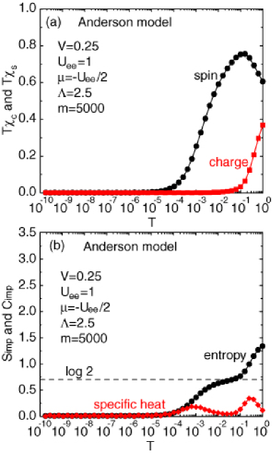
Figure 1: (Color online) (a) $T\chi_{\rm c}$ and $T\chi_{\rm s}$ vs. temperature for the Anderson model with $U_{\rm ee}=1$. (b) $S_{\rm imp}$ and $C_{\rm imp}$ vs. temperature for the Anderson model with $U_{\rm ee}=1$.

3 Kondo Behavior for $U_{\rm ee}\neq U_{\rm ph}$

3.1 Numerical results

First let us briefly review the results of the Anderson model, in order to clarify the effect of Holstein phonon. In Fig. 1(a), we show $T\chi_{\rm c}$ and $T\chi_{\rm s}$ for $U_{\rm ee}$=1. The charge susceptibility is rapidly suppressed due to the effect of on-site Coulomb interaction, while the spin susceptibility is increased. As is well known, in the Kondo system, the renormalization flow moves toward the strong-coupling regime in which the spin susceptibility is suppressed, through the local moment regime with enhanced spin susceptibility.

The Kondo behavior is clearly observed in the entropy and the specific heat. After the charge susceptibility is suppressed around at a temperature in the order of $U_{\rm ee}$, we can observe the local moment region with $\log 2$ between $0.01<T<0.1$. Then, the entropy of $\log 2$ is gradually released and around at $T\sim 10^{-4}$, it eventually goes to zero. We can see a clear peak in the specific heat around at $T\sim 10^{-3}$ due to the release of spin entropy $\log 2$. We define the Kondo temperature $T_{\rm K}^{(0)}$ of the Anderson model as a lower peak in the specific heat. It is well known that $T_{\rm K}^{(0)}$ is scaled by $e^{-1/(2\rho_{0}J_{0})}$, where the exchange interaction $J_{0}$ is given by $J_{0}$=$4V^{2}/U_{\rm ee}$ and $\rho_{0}$ is the density of states at the Fermi level. Although a peak in the specific heat does not indicate exactly the Kondo temperature, the effect of the prefactor is simply ignored here, since in this paper, we concentrate on the scaling relation when the parameters of the model are changed. Thus, we conventionally define $T_{\rm K}$ as the lower peak in the specific heat throughout this paper.

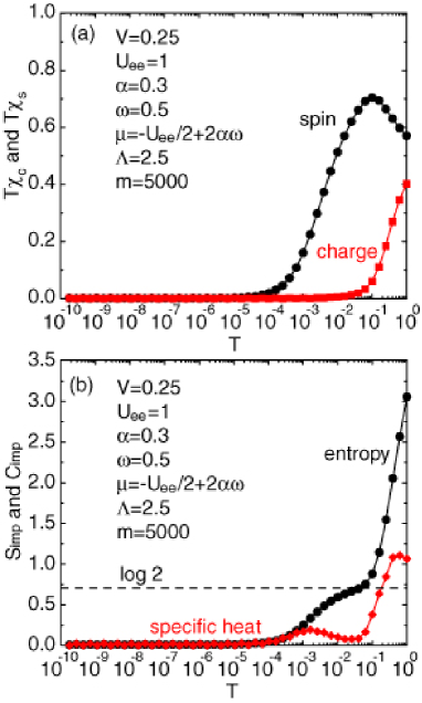
Figure 2: (Color online) (a) $T\chi_{\rm c}$ and $T\chi_{\rm s}$ vs. temperature for $\alpha$=0.3, $\omega$=0.5, and $U_{\rm ee}$=1. (b) $S_{\rm imp}$ and $C_{\rm imp}$ vs. temperature for the same parameters as (a).

Now let us show the results of the Anderson-Holstein model. First we consider the case in which the Coulomb interaction is dominant. In Fig. 2(a), we show the results for $T\chi_{\rm s}$ and $T\chi_{\rm c}$ for $U_{\rm ee}$=1, $\alpha$=0.3, and $\omega$=0.5. We note that in this case, $U_{\rm ph}$=0.3, which is smaller than $U_{\rm ee}$. We find that the charge susceptibility is rapidly suppressed around at $T\sim 0.03$. With decreasing temperature, the spin susceptibility is suppressed around at $T\sim 10^{-4}$. In Fig. 2(b), we show the entropy and specific heat for the same parameters as in Fig. 2(a). At high temperatures as $T>0.1$, we observe the entropy larger than $\log 4$ due to the low-lying phonon excitation states. Passing through the narrow local moment region, the entropy $\log 2$ is released and the peak appears in the specific heat. Note that the peak position is slightly shifted to the higher-temperature side in comparison with Fig. 1(b).

The overall features of Figs. 2 are quite similar to those of Figs. 1 except for the high-temperature region, since the situation is effectively understood by the Anderson model with reduced Coulomb repulsion $U_{\rm ee}-U_{\rm ph}$=0.7. As we will discuss later, due to the decrease of Coulomb interaction, the Kondo temperature is increased in comparison with that of the Anderson model with $U_{\rm ee}$=1.

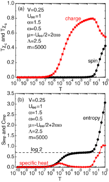
Figure 3: (Color online) (a) $T\chi_{\rm c}$ and $T\chi_{\rm s}$ vs. temperature for $\alpha$=1.5, $\omega$=0.5, and $U_{\rm ee}$=1. (b) $S_{\rm imp}$ and $C_{\rm imp}$ vs. temperature for the same parameters as (a).

Next we consider the situation with $U_{\rm ee}<U_{\rm ph}$. In Fig. 3(a), we show the results for $T\chi_{\rm s}$ and $T\chi_{\rm c}$ for $U_{\rm ee}$=1, $\alpha$=1.5, and $\omega$=0.5. In this case, we obtain $U_{\rm ph}$=1.5, leading to on-site attractive interaction with $U_{\rm ee}-U_{\rm ph}$=$-0.5$. Thus, in sharp contrast to Fig. 2(a), the spin susceptibility is first rapidly suppressed around at $T\sim 0.1$. With decreasing temperature, through the localized charge state, the charge susceptibility vanishes around at $T\sim 10^{-6}$.

In Fig. 3(b), we depict the entropy and specific heat for the same parameters as in Fig. 3(a). At high temperatures, we again observe that the entropy is larger than $\log 4$ due to the low-lying phonon states. We find the localized charge region with $\log 2$ between $10^{-4}<T<0.1$, originating from the double degeneracy of vacant and double occupied sites. With decreasing temperature, the entropy $\log 2$ is eventually released and a clear peak appears in the specific heat.

Due to the effective attractive interaction, we can find the Kondo behavior concerning charge degree of freedom for $U_{\rm ee}<U_{\rm ph}$. Since we are now considering the half-filling case, as mentioned above, vacant and double occupied states are degenerate and these states play roles of pseudo-spins. Thus, we can understand the occurrence of the Kondo-like behavior in the case of $U_{\rm ee}<U_{\rm ph}$. The difference in the magnitude of the Kondo temperature between the cases of $U_{\rm ee}>U_{\rm ph}$ and $U_{\rm ee}<U_{\rm ph}$ will be discussed in the next subsection.

3.2 Effective $s$-$d$ models

In the previous subsection, we have shown the NRG results for $U_{\rm ee}>U_{\rm ph}$ and $U_{\rm ee}<U_{\rm ph}$. Here let us discuss analytic expressions for $T_{\rm K}$. By using the second-order perturbation theory in terms of the hybridization, we can derive the effective $s$-$d$ model from the Anderson-Holstein model. There appear the virtual second-order processes concerning phonon excitations in addition to electronic excitations, which affect on the exchange interactions. The similar calculations have been done in the derivation of the effective model from the Hubbard-Holstein model. [27, 28, 29]

After some algebraic calculations, we obtain the effective $s$-$d$ models for $U_{\rm ee}>U_{\rm ph}$ and $U_{\rm ee}<U_{\rm ph}$, respectively, as

$$\begin{split}H^{\rm(s)}_{\rm s-d}&=\sum_{\mib{k}\sigma}\varepsilon_{\mib{k}}c_{\mib{k}\sigma}^{{\dagger}}c_{\mib{k}\sigma}\\ &+\sum_{{\mib k},{\mib k^{\prime}}}[J_{+}(c_{\mib{k}\uparrow}^{{\dagger}}c_{\mib{k^{\prime}}\uparrow}-c_{\mib{k}\downarrow}^{{\dagger}}c_{\mib{k^{\prime}}\downarrow})S_{z}\\ &+J_{+}(c_{\mib{k}\downarrow}^{{\dagger}}c_{\mib{k^{\prime}}\uparrow}S_{+}+c_{\mib{k}\uparrow}^{{\dagger}}c_{\mib{k^{\prime}}\downarrow}S_{-})],\end{split}$$ (12)

and

$$\begin{split}H^{\rm(c)}_{\rm s-d}&=\sum_{\mib{k}\sigma}\varepsilon_{\mib{k}}c_{\mib{k}\sigma}^{{\dagger}}c_{\mib{k}\sigma}\\ &+\sum_{{\mib k},{\mib k^{\prime}}}[J_{+}(c_{\mib{k}\uparrow}^{{\dagger}}c_{\mib{k^{\prime}}\uparrow}+c_{\mib{k}\downarrow}^{{\dagger}}c_{\mib{k^{\prime}}\downarrow}-1)\eta_{z}\\ &+J_{-}(c_{\mib{k}\uparrow}c_{\mib{k^{\prime}}\downarrow}\eta_{+}+c_{\mib{k}\downarrow}^{{\dagger}}c_{\mib{k^{\prime}}\uparrow}^{{\dagger}}\eta_{-})],\end{split}$$ (13)

where $S_{z}$=$(n_{\uparrow}-n_{\downarrow})/2$, $S_{+}$=$d_{\uparrow}^{{\dagger}}d_{\downarrow}$, $S_{-}$=$d_{\downarrow}^{{\dagger}}d_{\uparrow}$, $\eta_{z}$=$(|2\rangle\langle 2|-|0\rangle\langle 0|)/2$, $\eta_{+}$=$|2\rangle\langle 0|$, and $\eta_{-}$=$|0\rangle\langle 2|$ with $|2\rangle$=$d^{{\dagger}}_{\uparrow}d^{{\dagger}}_{\downarrow}|0\rangle$.

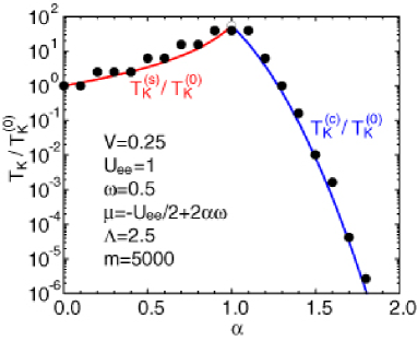
Figure 4: (Color online) Kondo temperature vs. $\alpha$ for $\omega$=0.5 and $U_{\rm ee}$=1. Solid symbols denotes numerical results while solid curves indicate analytic results of $T_{\rm K}^{\rm(c)}$ and $T_{\rm K}^{\rm(s)}$. The open circle at $\alpha$=1 indicates that the analytic results cannot be used at this point.

The exchange interactions are expressed as

$$J_{\pm}=4V^{2}e^{-\alpha}\sum_{\ell=0}^{\infty}\frac{(\pm\alpha)^{\ell}}{\ell!}\frac{1}{|U-U_{\rm ph}|+2\ell\omega}.$$ (14)

We note that this expression does not hold around at $U_{\rm ee}=U_{\rm ph}$. Note also that the longitudinal and transverse parts of $H^{\rm(c)}_{\rm s-d}$ are given by $J_{+}$ and $J_{-}$, respectively, while for $H^{\rm(s)}_{\rm s-d}$, both are given by $J_{+}$. The difference between $J_{+}$ and $J_{-}$ clearly appears in the asymptotic form for large $\alpha$ as $J_{+}\sim 1/\alpha$ and $J_{-}\sim e^{-2\alpha}/\alpha$. Namely, in the strong electron-phonon coupling region, $J_{-}$ decays very rapidly, while $J_{+}$ becomes small slowly. The smallness of $J_{-}$ for large $\alpha$ originates from the immobile nature of bi-polaron. Single polaron can be relatively mobile in comparison with bi-polaron.

Now we discuss the Kondo temperatures on the basis of the effective $s$-$d$ models. For the case of $U_{\rm ee}>U_{\rm ph}$, $H_{\rm s-d}^{\rm(s)}$ is the isotropic $s$-$d$ model and we can easily obtain

$$T^{\rm(s)}_{\rm K}=D{\rm exp}\Bigl{(}-\frac{1}{2\rho_{0}J_{+}}\Bigr{)}.$$ (15)

On the other hand, $H_{\rm s-d}^{\rm(c)}$ is the $s$-$d$ model with anisotropic exchange interaction. For this case, Shiba has obtained the explicit expression for the binding energy ${\tilde{E}}$.[30] When we define the Kondo temperature $T_{\rm K}$ as $T_{\rm K}=-{\tilde{E}}$, we obtain

$$T^{\rm(c)}_{\rm K}=D{\rm exp}\Biggl{[}\frac{-1}{2\rho_{0}\sqrt{J_{+}^{2}-J_{-}^{2}}}{\rm tanh}^{-1}\Bigl{(}\frac{\sqrt{J_{+}^{2}-J_{-}^{2}}}{J_{+}}\Bigr{)}\Biggr{]}.$$ (16)

In Fig. 4, we depict $T_{\rm K}/T_{\rm K}^{(0)}$ vs. $\alpha$. Numerical results are shown by solid symbols. Note that $T_{\rm K}$ as well as $T_{\rm K}^{(0)}$ in the numerical results is defined as a temperature which shows the peak in the specific heat. Analytic results for the $s$-$d$ models are depicted by solid curves, which indicate eqs. (15) and (16) divided by $T_{\rm K}^{(0)}$. We find that the numerical results agree well with the analytic curves for $H_{\rm s-d}^{\rm(s)}$ and $H_{\rm s-d}^{\rm(c)}$. Note that the numerical results seem to scatter due to the effect of discrete temperature $\Lambda^{-(N-1)/2}$, but all the results are considered to be in the error-bars.

As mentioned above, for $U_{\rm ee}<U_{\rm ph}$, the effective $s$-$d$ model becomes highly anisotropic for large $\alpha$. Since the transverse part is exponentially small, the interaction part of $H_{\rm s-d}^{\rm(c)}$ becomes Ising-like and the Kondo temperature is rapidly suppressed. Thus, the plot of $T_{\rm K}$ vs. $\alpha$ is asymmetric at the center of $\alpha$=1 ($U_{\rm ee}$=$U_{\rm ph}$). Note also that two analytic curves seem to converge to a value similar to the numerical result at $\alpha$=1, but as mentioned above, the expression of $T_{\rm K}$ does not hold around at $U_{\rm ee}$=$U_{\rm ph}$. The Kondo behavior in the repulsion-attraction competing region with $U_{\rm ee}\approx U_{\rm ph}$ will be separately discussed in the next section.

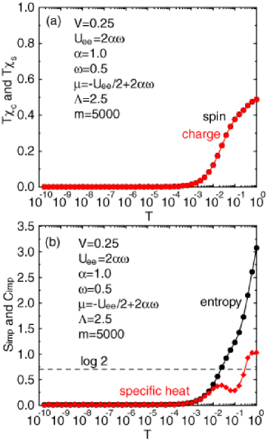
Figure 5: (Color online) (a) $T\chi_{\rm c}$ and $T\chi_{\rm s}$ vs. temperature for $\alpha$=1 and $\omega$=0.5 with $U_{\rm ee}$=$2\alpha\omega$. (b) $S_{\rm imp}$ and $C_{\rm imp}$ vs. temperature for the same parameters as (a).

4 Kondo Behavior in the Competing Region

Now we focus on the case of $U_{\rm ee}=U_{\rm ph}$. In Fig. 5(a), we show the results for $T\chi_{\rm s}$ and $T\chi_{\rm c}$ for $\alpha$=1, $U_{\rm ee}$=1, and $\omega$=0.5. As naively expected from the cancellation of the on-site interaction, the situation is considered to be understood by the non-interacting model. In fact, as shown in Fig. 5(a), it is very difficult to distinguish the charge and spin susceptibilities, indicating that the interaction effect is virtually ignored.

In Fig. 5(b), the entropy and specific heat are shown for the same parameters as in Fig. 5(a). At high temperatures as $T>0.1$, in common with the cases of $U_{\rm ee}\neq U_{\rm ph}$, we find that the entropy is larger than $\log 4$ due to the low-lying phonon states. We note that the entropy gradually goes to zero without showing the region of $\log 2$. We can see the peak in the specific heat around at $T\sim 0.01$, which has been assigned as the Kondo temperature in Fig. 4. However, this Kondo-like behavior is not due to Coulomb interaction, but it originates from the hybridization in the non-interacting Anderson model. This point will be discussed later again.

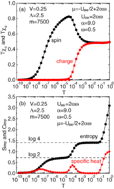
Figure 6: (Color online) (a) $T\chi_{\rm c}$ and $T\chi_{\rm s}$ vs. temperature for $\alpha$=9 and $\omega$=0.5 with $U_{\rm ee}$=$2\alpha\omega$. (b) $S_{\rm imp}$ and $C_{\rm imp}$ vs. temperature for the same parameters as (a). Note that in this case, we increase $m$ up to 7500, since convergence becomes worse due to the strong-coupling nature.

Next we increase the value of $\alpha$ by keeping the relation of $U_{\rm ee}=U_{\rm ph}$. In Fig. 6(a), we show the results for $T\chi_{\rm s}$ and $T\chi_{\rm c}$ for $\alpha$=9, $U_{\rm ee}$=$2\alpha\omega$, and $\omega$=0.5. From the viewpoint of the comparison with actual materials, the value of $\alpha$=9 seems to be unrealistically large, but we consider such a situation in order to complete the discussion from the theoretical viewpoint. As naively expected from the cancellation of on-site interaction, the situation can be understood from the non-interacting model, but in the strong-coupling case, the results clearly show the interaction effect. For $T>10^{-3}$, $T\chi_{\rm c}$ and $T\chi_{\rm s}$ takes a constant value of 0.5. This region can be interpreted as the free orbital regime, described by the conduction electron systems.[25] Around at $T\sim 10^{-3}$, spin and charge response begin to be separated from each other. The charge susceptibility is rapidly suppressed, while the spin susceptibility grows up, suggesting the local moment regime. After that, the spin susceptibility is gradually suppressed and it eventually goes to zero around at $T\sim 10^{-9}$, entering the strong-coupling regime.

The above behavior can be clearly found in the entropy and the specific heat, as shown in Fig. 6(b). The high-temperature behavior is almost the same as that in Fig. 5(b). For $0.1<T<10^{-4}$, we clearly observe the region of $\log 4$ due to the four-fold degeneracy of vacant, spin-up, spin-down, and double occupied states, corresponding to the free-orbital regime. Then, the entropy of $\log 2$ relevant to charge degree of freedom is released and a peak is formed in the specific heat. Finally, the residual entropy of $\log 2$ for spin degree of freedom is released and we find another peak in the specific heat.

From the above numerical results, we deduce that the case of $U_{\rm ee}=U_{\rm ph}$ is described by the Anderson model with effective on-site repulsive interaction. From ${\tilde{H}}$, eq. (11), we propose the polaronic Anderson model, given by

$$\begin{split}H_{\rm eff}&=\sum_{{\bf k}\sigma}\varepsilon_{\bf{k}}c_{\bf{k}\sigma}^{{\dagger}}c_{\bf{k}\sigma}+\sum_{\bf{k}\sigma}(V_{\rm eff}c_{\bf{k}\sigma}^{{\dagger}}d_{\sigma}+{\rm h.c.})\\ &+U_{\rm eff}n_{\uparrow}n_{\downarrow}+\mu_{\rm eff}\rho,\end{split}$$ (17)

where $V_{\rm eff}$ is the hybridization for polarons, $U_{\rm eff}$ is the residual Coulomb interaction among polarons, and $\mu_{\rm eff}$ is the chemical potential for polarons, given by $\mu_{\rm eff}$=$-U_{\rm eff}/2$.

By taking the average over the zero-phonon state, we obtain $V_{\rm eff}$ as $V_{\rm eff}$=$V\langle 0|X|0\rangle$=$Ve^{-\alpha/2}$. However, we cannot hit upon an idea to derive the analytic form of $U_{\rm eff}$. Then, we resort to a numerical method to determine $U_{\rm eff}$ so as to reproduce the average value of double occupancy $\langle n_{\uparrow}n_{\downarrow}\rangle$ of $H$.

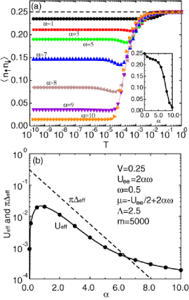
Figure 7: (Color online) (a) $\langle n_{\uparrow}n_{\downarrow}\rangle$ vs. temperature for several values of $\alpha$ with $\omega$=0.5 and $U_{\rm ee}$=$2\alpha\omega$. Inset shows $\langle n_{\uparrow}n_{\downarrow}\rangle$ at the lowest temperature in the present NRG calculations. (b) $\Delta_{\rm eff}$ and $U_{\rm eff}$ vs. $\alpha$ for $\omega$=0.5 and $U_{\rm ee}$=$2\alpha\omega$.

In Fig. 7(a), we show $\langle n_{\uparrow}n_{\downarrow}\rangle$ for several values of $\alpha$ with $U_{\rm ee}$=$2\alpha\omega$. In the inset, we depict $\langle n_{\uparrow}n_{\downarrow}\rangle$ at the lowest temperature which we can reach in the present NRG calculation. Irrespective of the vales of $\alpha$, in the high-temperature region as $T>10^{-3}$, $\langle n_{\uparrow}n_{\downarrow}\rangle$ takes the value near the non-interacting one, 0.25. When we further decrease the temperature, for $\alpha<6$, $\langle n_{\uparrow}n_{\downarrow}\rangle$ is not largely suppressed and it keeps the value about 0.2 even at low temperatures. However, for $\alpha>6$, it is rapidly suppressed and takes the value much smaller than 0.25. In fact, as shown in the inset, the low-temperature value of $\langle n_{\uparrow}n_{\downarrow}\rangle$ is rapidly suppressed around at $\alpha\sim 6$.

Readers may feel it strange that the double occupancy is so suppressed, in spite of the fact that the on-site interaction exactly vanishes at $U_{\rm ee}=U_{\rm ph}$. As mentioned in the explanation of the effective $s$-$d$ model, bi-polaron has immobile nature in comparison with single polaron for large $\alpha$. Due to the difference in the mobility between polaron and bi-polaron, single polaron state has the energy gain of the exchange interaction, while bi-polaron cannot. Thus, the single polaron state is favored in the strong-coupling region, leading to the effective occurrence of the residual repulsion between polarons.

By changing the values of $U_{\rm eff}$ for each values of $\alpha$, we repeat the NRG calculations for $H_{\rm eff}$, until we can reproduce the low-temperature value of $\langle n_{\uparrow}n_{\downarrow}\rangle$ of $H$. The results are shown by solid symbols in Fig. 7(b). In order to understand intuitively the extent of correlation effect, we also depict the line of $\pi\Delta_{\rm eff}$, where $\Delta_{\rm eff}$ is the width of the virtual bound state, expressed as $\Delta_{\rm eff}$=$\pi\rho_{0}V_{\rm eff}^{2}$=$\pi\rho_{0}V^{2}e^{-\alpha}$. Note that the expansion parameter of the Anderson model is given by $U_{\rm eff}/(\pi\Delta_{\rm eff})$. [31, 32, 33, 34] For $\alpha<6.5$, we observe that $U_{\rm eff}$ is smaller than $\pi\Delta_{\rm eff}$, suggesting that the peak in the specific heat should be determined by $\Delta_{\rm eff}$. For large $\alpha$, on the other hand, $U_{\rm eff}$ is still small, but $\Delta_{\rm eff}$ is exponentially reduced, as observed in Fig. 7(b). Then, in this region, we expect that the correlation effect becomes significant.

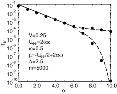
Figure 8: $T_{\rm K}$ vs. $\alpha$ for $\omega$=0.5 and $U_{\rm ee}$=$2\alpha\omega$.

In Fig. 8, we summarize the numerical results for the peak temperature in the specific heat with the fitting curve deduced from the polaron Anderson model.[35] For $\alpha<6.5$, as described above, the NRG results are simply scaled by $\Delta_{\rm eff}$. For $\alpha>6.5$, as typically found in Figs. 6, we obtain clear two peaks in the specific heat. The higher peak concerning charge degree of freedom should be characterized by $U_{\rm eff}$, while the lower one indicates the characteristic temperature of the standard Kondo effect, given by $e^{-1/(2\rho_{0}J_{\rm eff})}$ with $J_{\rm eff}$=$4V_{\rm eff}^{2}/U_{\rm eff}$. By adjusting appropriately numerical prefactors at $\alpha$=7, we can actually fit the NRG results by $U_{\rm eff}$ and $e^{-1/(2\rho_{0}J_{\rm eff})}$. We believe that the success of this fitting suggests the effectiveness of the polaron Anderson model, which describes the low-energy states of the Anderson-Holstein model in the competing region of $U_{\rm ee}\approx U_{\rm ph}$.

5 Discussion and Summary

We have clarified the Kondo behavior of the Anderson-Holstein model by using the NRG method. It has been clearly shown that the results are categorized into three classes labeled by $U_{\rm ee}>U_{\rm ph}$, $U_{\rm ee}<U_{\rm ph}$, and $U_{\rm ee}\approx U_{\rm ph}$. For $U_{\rm ee}>U_{\rm ph}$, the standard magnetic Kondo phenomenon occurs with the reduced Coulomb interaction, suggesting the increase of the Kondo temperature in comparison with that of the Anderson model without the electron-phonon interaction. For $U_{\rm ee}<U_{\rm ph}$, the charge Kondo effect occurs and the Kondo temperature is decreased with the increase of electron-phonon coupling constant, since the relevant exchange interaction is decreased when we increase $\alpha$. Note that the effective $s$-$d$ model for this case becomes highly anisotropic, since the transverse part is related to the bi-polaron motion with immobile nature in comparison with single polaron.

Around at $U_{\rm ee}\approx U_{\rm ph}$, the Kondo temperature is maximized, but for small $\alpha$, the characteristic energy is simply given by the width of the virtual bound state of the non-interacting Anderson model. In this sense, we should not call the peak in the specific heat as the Kondo temperature for small $\alpha$, but the Kondo-like behavior occurs at relatively high temperature, when the strong electron-phonon interaction competes with Coulomb interaction. We may consider possible relevance of this scenario to the enhanced Kondo temperature observed in molecular quantum dots. For larger $\alpha$, the effect of residual polaron repulsion becomes significant, since the polaron hybridization is exponentially suppressed. Then, we have found the Kondo singlet formation, through the free-orbital and local moment regimes.

Finally, we provide a comment on the different effect of the phonon mode on the Kondo temperature. In this paper, we have concentrated on the Holstein phonon and stressed the enhancement of the Kondo temperature. However, this enhancement depends on the feature of relevant phonon. For instance, for the case of Jahn-Teller phonon, the Kondo temperature is monotonically decreased with the increase of the electron-phonon coupling constant. [12, 13] For Jahn-Teller phonon, the local electron-phonon state has double degeneracy originating from clockwise and anti-clockwise rotational phonon mode. Such geometrical degree of freedom is characterized by $J$=$\pm 1/2$, where $J$ is total angular moment, composed of electron orbital and phonon angular moments. The conduction electrons must screen phonon angular moment in addition to electron orbital moment to form the singlet ground state with $J$=0. Thus, the Kondo temperature is decreased when we increase $\alpha$.

In summary, we have discussed the Kondo effect of the Anderson-Holstein model. We have observed that the Kondo behavior can be explained by the isotropic $s$-$d$ model for $U_{\rm ee}>U_{\rm ph}$, the polaron Anderson model for $U_{\rm ee}\approx U_{\rm ph}$, and the anisotropic $s$-$d$ model for $U_{\rm ee}<U_{\rm ph}$. The Kondo behavior has been found to be enhanced when $U$ competes with $U_{\rm ph}$.

References

- [1] Kondo effect and its related phenomena have been reviewed in J. Phys. Soc. Jpn. 74 (2005) 1-238.
- [2] J. Kondo: Prog. Theor. Phys. 32 (1964) 37.
- [3] J. Kondo: Physica 84B (1976) 40.
- [4] J. Kondo: Physica 84B (1976) 207.
- [5] K. Vladar and A. Zawadowski: Phys. Rev. B 28 (1983) 1564.
- [6] K. Vladar and A. Zawadowski: Phys. Rev. B 28 (1983) 1582.
- [7] S. Yotsuhashi, M. Kojima, H. Kusunose and K. Miyake: J. Phys. Soc. Jpn. 74 (2005) 49.
- [8] K. Hattori, Y. Hirayama and K. Miyake: J. Phys. Soc. Jpn. 74 (2005) 3306.
- [9] K. Hattori, Y. Hirayama and K. Miyake: Proc. 5th Int. Symp. ASR-WYP-2005: Advances in the Physics and Chemistry of Actinide Compounds, J. Phys. Soc. Jpn. 75 (2006) Suppl., p. 238.
- [10] S. Sanada, Y. Aoki, H. Aoki, A. Tsuchiya, D. Kikuchi, H. Sugawara and H. Sato: J. Phys. Soc. Jpn. 74 (2005) 246.
- [11] W. M. Yuhasz, N. A. Frederick, P.-C. Ho, N. P. Butch, B. J. Taylor, T. A. Sayles, M. B. Maple, J. B. Betts, A. H. Lacerda, P. Rogl and G. Giester: Phys. Rev. B 71 (2005) 104402.
- [12] T. Hotta: Phys. Rev. Lett. 96 (2006) 197201.
- [13] T. Hotta: J. Phys. Soc. Jpn. 76 (2007) 023705.
- [14] T. Hotta: J. Magn. Magn. Mater. 310 (2007) 1691.
- [15] T. Hotta: J. Phys. Soc. Jpn. 76 (2007) 034713.
- [16] A. C. Hewson and D. Meyer: J. Phys.: Condens. Matter. 14 (2002) 427.
- [17] G. S. Jeon, T. -H. Park and H. -Y. Choi: Phys. Rev. B 68 (2003) 045106.
- [18] H. C. Lee and H. -Y. Choi: Phys. Rev. B 69 (2004) 075109.
- [19] K. Mitsumoto and Y. Ōno: Physica C 426-431 (2005) 330.
- [20] L. H. Yu, Z. K. Keane, J. W. Ciszek, L. Cheng, M. P. Stewart, J. M. Tour and D. Natelson: Phys. Rev. Lett. 93 (2004) 266802.
- [21] L. H. Yu, Z. K. Keane, J. W. Ciszek, L. Cheng, J. M. Tour, T. Baruah, M. R. Pederson and D. Natelson: Phys. Rev. Lett. 95 (2005) 245803.
- [22] P. S. Cornaglia, H. Ness and D. R. Grempel: Phys. Rev. Lett. 93 (2004) 147201.
- [23] P. S. Cornaglia, D. R. Grempel and H. Ness: Phys. Rev. B 71 (2005) 075320.
- [24] P. S. Cornaglia and D. R. Grempel: Phys. Rev. B 71 (2005) 245326.
- [25] H. R. Krishna-murthy, J. W. Wilkins and K. G. Wilson: Phys. Rev. B 21 (1980) 1003.
- [26] I. G. Lang and Yu. A . Firsov: Zh. Eksp. Theor. Fiz. 43 (1962) 1843 [Sov. Phys. -JETP 16 (1963) 1301].
- [27] T. Hotta and Y. Takada: Phys. Rev. Lett. 76 (1996) 3180.
- [28] T. Hotta and Y. Takada: J. Phys. Soc. Jpn. 65 (1996) 2922.
- [29] T. Hotta and Y. Takada: Phys. Rev. B 56 (1997) 13916.
- [30] H. Shiba: Prog. Theor. Phys. 43 (1970) 601.
- [31] K. Yamada and K. Yoshida: Prog. Thoer. Phys. Suppl. 46 (1970) 244.
- [32] K. Yamada: Prog. Thoer. Phys. 53 (1975) 970.
- [33] K. Yoshida and K. Yamada: Prog. Thoer. Phys. 53 (1975) 1286.
- [34] K. Yamada: Prog. Thoer. Phys. 54 (1975) 316.
- [35] T. Hotta: submitted to Physica B.