Effects of an oscillating field on pattern formation in a ferromagnetic thin film: Analysis of patterns traveling at a low velocity

Abstract

Magnetic domain patterns under an oscillating field are studied theoretically by using a simple Ising-like model. We propose two ways to investigate the effects of the oscillating field. The first one leads to a model in which rapidly oscillating terms are averaged out and the model can explain the existence of the maximum amplitude of the field for the appearance of patterns. The second one leads to a model that includes the delay of the response to the field and the model suggests the existence of a traveling pattern which moves very slowly compared with the time scale of the driving field.

I Introduction

Rapidly driven systems have received considerable attention these days. Under a rapidly oscillating field, a state which is unstable in the absence of the oscillating field can be stabilized. One of the most simple and well-known examples is Kapitza’s inverted pendulum and Landau and Lifshitz generalized the problem landau . Their method has recently been applied to classical and quantum dynamics in periodically driven systems rahav03 ; rahav05 . The method is also applied to stabilization of a matter-wave soliton in two-dimensional Bose-Einstein condensates without an external trap saito ; abdullaev ; liu .

Magnetic domain patterns in a uniaxial ferromagnetic thin film, which usually show a labyrinth structure, exhibit various kinds of structures under an oscillating field. For example, the labyrinth structure changes into a parallel-stripe structure for a certain field miura ; mino . In some other cases, several types of lattice structures can appear tsuka .

In this paper, we develop effective theories for slow motion of magnetic domain patterns under a rapidly oscillating field. Especially, we focus on traveling patterns as an example of slowly moving patterns. So far, there were few effective theories to describe such a slowly traveling pattern under a rapidly oscillating field. In experiments on a garnet thin film, we can observe a parallel-stripe pattern traveling very slowly compared with the time scale of the field in some cases mino_p . A traveling mazelike pattern like Fig. 1 is also found in our numerical simulations.

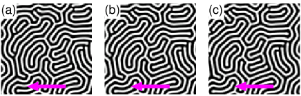
Figure 1: Snapshots of a traveling pattern under an oscillating field after (a) 5000 cycles, (b) 10000 cycles, and (c) 15000 cycles. The whole pattern is traveling to the left. The details are described in Appendix A.

Although traveling patterns appear in various kinds of systems, most works about them have been limited to the systems in the absence of an oscillating field malomed ; coullet ; douady ; fauvePRL ; price ; lega ; okuzono ; sagues . The mechanism of such traveling patterns in one-dimensional (1D) systems was intensively studied in the 1980s as drift instabilities or parity-breaking instabilities malomed ; coullet ; douady ; fauvePRL . In Ref. malomed , secondary instabilities were discussed for several similar equations. By contrast, the authors of Refs. coullet ; douady ; fauvePRL gave no particular equation at first, but they considered symmetries of the system and assumed the form of the solution before deriving their equations. Almost 10 years after those papers, Price studied traveling patterns in 2D scalar nonlinear neural fields where the nonlinearity is purely cubic and discussed constraints on the neural field structure and parameters to support traveling patterns price . He suggested that Swift-Hohenberg-type models will not support traveling patterns. However, moving patterns were actually observed in numerical simulations for a general complex Swift-Hohenberg equation in Ref. lega . Our model has similar properties to those of the (real) Swift-Hohenberg equation. We will not use the method of Ref. price but that of Ref. malomed to explore the existence of a traveling pattern in a ferromagnetic thin film.

In fact, recently, domain walls under a rapidly oscillating field have been studied michaelis ; kirakosyan . Michaelis et al. discussed the effects of rapid periodic oscillation of parameters in a Ginzburg-Landau (GL) equation by applying a multiscale technique and derived the averaged GL equation michaelis ; Kirakosyan et al. derived the averaged Landau-Lifshitz equation by employing the multi-time-scale expansion technique kirakosyan . In those papers, they took into account higher harmonic oscillations. Although their methods cannot be directly applied to our model, our methods correspond to the lowest orders of their multi-time-scale expansions.

Our model is a simple 2D Ising-like model (see Refs. jagla04 ; jagla05 ; kudoE ; kudoS , and references therein), which has been used to simulate magnetic domain patterns. The numerical results simulated by the model show very similar properties to experimental ones jagla04 ; jagla05 ; kudoE ; kudoS . We consider a scalar field $\phi(\bm{r})$, where $\bm{r}=(x,y)$. The positive and negative values of $\phi(\bm{r})$ correspond to the up and down spins, respectively. The Hamiltonian consists of four energy terms: Uniaxial-anisotropy energy $H_{\rm ani}$, exchange interactions $H_{J}$, dipolar interactions $H_{\rm di}$, and interactions with the external field $H_{\rm ex}$. The anisotropy energy is given by

$$H_{\rm ani}=\alpha\int{\rm d}\bm{r}\left(-\frac{\phi(\bm{r})^{2}}{2}+\frac{\phi(\bm{r})^{4}}{4}\right).$$ (1)

It implies that the anisotropy energy prefers the values $\phi(\bm{r})=\pm 1$. The exchange and dipolar interactions are described by

$$H_{J}=\beta\int{\rm d}\bm{r}\frac{|\nabla\phi(\bm{r})|^{2}}{2}$$ (2)

and

$$H_{\rm di}=\gamma\int{\rm d}\bm{r}{\rm d}\bm{r}^{\prime}\phi(\bm{r})\phi(\bm{r}^{\prime})G(\bm{r},\bm{r}^{\prime}),$$ (3)

respectively. Here, $G(\bm{r},\bm{r}^{\prime})\sim|\bm{r}-\bm{r}^{\prime}|^{-3}$ at long distances. The exchange interactions imply that $\phi(\bm{r})$ tends to have the same value as neighbors. On the other hand, the dipolar interactions imply that $\phi(\bm{r})$ tends to have the opposite sign to the values in a region at a long distance. Namely, $H_{J}$ and $H_{\rm di}$ may be interpreted as short-range attractive and long-range repulsive interactions, respectively. Their competition leads to a domain structure with a characteristic length. The term from the interactions with the external field is given by

$$H_{\rm ex}=-h(t)\int{\rm d}\bm{r}\phi(\bm{r}).$$ (4)

Here, we consider a spatially homogeneous and rapidly oscillating field:

$$h(t)=h_{0}\sin\omega t.$$ (5)

From Eqs. (1)–(4), the dynamical equation of the model is described by

$$\frac{\partial\phi(\bm{r})}{\partial t} = -L_{0}\frac{\delta(H_{\rm ani}+H_{J}+H_{\rm di}+{H_{\rm ex}})}{\delta\phi(\bm{r})}$$ (6)

$$= L_{0}\biggl{\{}\alpha[\phi(\bm{r})-\phi(\bm{r})^{3}]+\beta\nabla^{2}\phi(\bm{r})-\gamma\int{\rm d}\bm{r}^{\prime}\phi(\bm{r}^{\prime})G(\bm{r},\bm{r}^{\prime})+h(t)\bigg{\}}.$$

Hereafter, we fix $L_{0}=1$ and give the parameters $\alpha$, $\beta$, $\gamma$, and $h_{0}$ as positive values.

In this paper, we propose two approximation methods to obtain the dynamical equation for slow motion. In both methods, we apply a part of Kapitza’s idea that the dynamics under a rapidly oscillating field can be separated into a rapidly oscillating part and a slowly varying part landau . In Sec. II, we derive the model whose rapidly oscillating part is averaged out on the basis of the Kapitza’s idea about the time average of the fast motion. In Sec. III, we derive another model for the slow motion, considering the delay of the response to the field instead of taking a time average. After the derivation of the models, the instabilities of traveling patterns are investigated in both Secs. II and III. We discuss the details about the existence of a traveling pattern in Sec. IV. Conclusions are given in Sec. V.

II Time-averaged model

First of all, we assume that the variable $\phi(\bm{r})$ can be separated into two parts:

$$\phi(\bm{r},t)=\Phi(\bm{r},t)+\phi_{0}(t).$$ (7)

Here, $\Phi(\bm{r},t)$ is a slowly varying term and $\phi_{0}(t)$ is a rapidly oscillating space-independent term. Substituting Eq. (7) into Eq. (6), we obtain

$$\frac{\partial\Phi(\bm{r})}{\partial t}+\dot{\phi_{0}}=\alpha\left[(\Phi(\bm{r})+\phi_{0})-(\Phi(\bm{r})+\phi_{0})^{3}\right]+\beta\nabla^{2}(\Phi(\bm{r})+\phi_{0})-\gamma\int{\rm d}\bm{r}^{\prime}(\Phi(\bm{r}^{\prime})+\phi_{0})G(\bm{r},\bm{r}^{\prime})+h(t).$$ (8)

Let us consider only the rapidly oscillating space-independent part; then we have

$$\dot{\phi_{0}}=\alpha(\phi_{0}-\phi_{0}^{3})-\gamma\phi_{0}\int{\rm d}\bm{r}^{\prime}G(\bm{r}^{\prime},0)+h(t).$$ (9)

Here, we define $G(\bm{r},0)\equiv 1/|\bm{r}|^{3}$. Then, the integral in Eq. (9) is a constant, $a_{0}$:

$$a_{0}=2\pi\int_{d}^{\infty}\frac{{\rm d}r}{r^{2}}.$$ (10)

Here, $d$ is the cutoff length to prevent the divergence for $d\to 0$. It is also interpreted as the lower limit of the dipolar interactions. The solution of Eq. (9) should have the following form:

$$\phi_{0}=\rho_{0}\sin(\omega t+\delta),$$ (11)

where $\delta$ is a phase shift which comes from the delay of the response to the field. Substituting Eq. (11) into Eq. (9) and omitting high-order harmonics (i.e. $\sin 3\omega t$), we have

$$\omega\rho_{0}\cos(\omega t+\delta)=\eta_{0}\rho_{0}\sin(\omega t+\delta)-\frac{3}{4}\alpha\rho_{0}^{3}\sin(\omega t+\delta)+h_{0}\sin\omega t,$$ (12)

where $\eta_{0}=\alpha-\gamma a_{0}$. From Eq. (12), a pair of simultaneous equations is obtained:

$$-\omega\rho_{0}\sin\delta = \left(\eta_{0}-\frac{3}{4}\alpha\rho_{0}^{2}\right)\rho_{0}\cos\delta+h_{0},$$ (13a)

$$\omega\rho_{0}\cos\delta = \left(\eta_{0}-\frac{3}{4}\alpha\rho_{0}^{2}\right)\rho_{0}\sin\delta.$$ (13b)

Eliminating $\delta$ from Eq. (13), we obtain a cubic equation of $X\equiv\rho_{0}^{2}$:

$$\frac{9}{16}\alpha^{2}X^{3}-\frac{3}{2}\alpha\eta_{0}X^{2}+(\omega^{2}+\eta_{0}^{2})X=h_{0}^{2}.$$ (14)

Therefore, $\rho_{0}$ can be evaluated from Eq. (14) if the parameters $\alpha$, $\eta_{0}$, $\omega$, and $h_{0}$ are given.

Now, let us think about the slowly varying part. After substituting Eq. (11) into Eq. (8), we average out the rapid oscillation, closely following Kapitza’s idea. Then, we obtain an equation for slowly varying domain patterns:

$$\frac{\partial\Phi(\bm{r})}{\partial t}=\alpha\left(\Phi(\bm{r})-\Phi(\bm{r})^{3}\right)-\frac{3}{2}\alpha\rho_{0}^{2}\Phi(\bm{r})+\beta\nabla^{2}\Phi(\bm{r})-\gamma\int{\rm d}\bm{r}^{\prime}\Phi(\bm{r}^{\prime})G(\bm{r},\bm{r}^{\prime}).$$ (15)

The second term on the right hand side of Eq. (15) is an extra term due to the time average. This term is essential to explore the effects of the rapidly oscillating field.

On the basis of Eq. (15), we will analyze the possibility of patterns traveling at a low velocity. Let us first choose the most simple moving stripe-type solution for Eq. (15):

$$\Phi(\bm{r},t)=A_{0}(t)+A_{1}(t)\sin(kx+b(t)).$$ (16)

Substituting Eq. (16) into Eq. (15) and omitting high-order harmonics, we have

$$\dot{A}_{0}+\dot{A}_{1}\sin(kx+b) +\dot{b}A_{1}\cos(kx+b)=\eta_{0}^{\prime}A_{0}+\eta_{1}^{\prime}A_{1}\sin(kx+b)$$ (17)

$$-\alpha\left[A_{0}^{3}+3A_{0}^{2}A_{1}\sin(kx+b)+\frac{3}{2}A_{0}A_{1}^{2}+\frac{3}{4}A_{1}^{3}\sin(kx+b)\right].$$

Here,

$$\eta_{0}^{\prime} = \left(1-\frac{3}{2}\rho_{0}^{2}\right)\alpha-\gamma a_{0},$$ (18a)

$$\eta_{1}^{\prime} = \left(1-\frac{3}{2}\rho_{0}^{2}\right)\alpha-\beta k^{2}-\gamma(a_{0}-a_{1}k),$$ (18b)

with $a_{0}$ given by Eq. (10), $a_{1}=2\pi$, and $k=|\bm{k}|$. Equation (17) leads to the following equations:

$$\dot{A}_{0} = \eta_{0}^{\prime}A_{0}-\alpha\left(A_{0}^{3}+\frac{3}{2}A_{0}A_{1}^{2}\right),$$ (19a)

$$\dot{A}_{1} = \eta_{1}^{\prime}A_{1}-\alpha\left(3A_{0}^{2}A_{1}+\frac{3}{4}A_{1}^{3}\right),$$ (19b)

$$\dot{b} = 0.$$ (19c)

Equation (19c) implies that the phase $b(t)$ in Eq. (16) shows no time dependence and that there is no traveling pattern with the simplest form like Eq. (16).

Next, let us consider a more generalized solution by incorporating the second harmonics:

$$\Phi(\bm{r},t)=A_{0}(t)+A_{1}(t)\sin(kx+b(t))+A_{21}\cos[2(kx+b(t))]+A_{22}\sin[2(kx+b(t))].$$ (20)

Substituting Eq. (20) into Eq. (15) leads to the following equations:

$$\dot{A}_{0} = \eta_{0}^{\prime}A_{0}-\alpha\left(A_{0}^{3}+\frac{3}{2}A_{0}A_{1}^{2}+\frac{3}{2}A_{0}A_{21}^{2}+\frac{3}{2}A_{0}A_{22}^{2}-\frac{3}{4}A_{1}^{2}A_{21}\right),$$ (21a)

$$\dot{A}_{1} = \eta_{1}^{\prime}A_{1}-\alpha\left(\frac{3}{4}A_{1}^{3}+3A_{0}^{2}A_{1}+\frac{3}{2}A_{1}A_{21}^{2}+\frac{3}{2}A_{1}A_{22}^{2}-3A_{0}A_{1}A_{21}\right),$$ (21b)

$$\dot{A}_{21} = \eta_{2}^{\prime}A_{21}-\alpha\left(\frac{3}{4}A_{21}^{3}-\frac{3}{2}A_{0}A_{1}^{2}+3A_{0}^{2}A_{21}+\frac{3}{2}A_{1}^{2}A_{21}+\frac{3}{4}A_{21}A_{22}^{2}-6A_{0}A_{22}^{2}\right),$$ (21c)

$$\dot{A}_{22} = \eta_{2}^{\prime}A_{22}-\alpha\left(\frac{3}{4}A_{22}^{3}+3A_{0}^{2}A_{22}+\frac{3}{4}A_{21}^{2}A_{22}+\frac{3}{2}A_{1}^{2}A_{22}+6A_{0}A_{21}A_{22}\right),$$ (21d)

and

$$\dot{b}=-3\alpha A_{0}A_{22}.$$ (22)

Here, $\eta_{0}^{\prime}$ and $\eta_{1}^{\prime}$ are given by Eq. (18), and

$$\eta_{2}^{\prime}=\left(1-\frac{3}{2}\rho_{0}^{2}\right)\alpha-4\beta k^{2}-\gamma(a_{0}-2a_{1}k).$$ (23)

This time, Eq (22) implies that there can be a traveling pattern if $A_{0}\neq 0$ and $A_{22}\neq 0$.

Now let us find a stationary point (SP) of Eq. (21) where $A_{0}=0$ or $A_{22}=0$, and examine its linear stability. If the SP is unstable and both $A_{0}$ and $A_{22}$ grow from zero, the pattern can start to travel. For the parameter values used to obtain Fig. 1, however, there are no SPs except for ones with $A_{0}=A_{21}=A_{22}=0$. We should note $A_{1}=0$ or $A_{1}^{2}=4\eta_{1}^{\prime}/3\alpha$ at the SPs with $A_{0}=A_{21}=A_{22}=0$. Since $A_{1}$ must be real, $\eta_{1}^{\prime}>0$. Namely,

$$\rho_{0}^{2}<\frac{2}{3\alpha}\left[\alpha-\beta k^{2}-\gamma(a_{0}-a_{1}k)\right].$$ (24)

This condition gives an estimate of the maximum value of the field amplitude $h_{0}$ to observe a nonuniform pattern, as $h_{0}$ proves to be a monotonic function of $\rho_{0}$ for the parameter values in Fig. 1. In other words, if Eq. (24) is not satisfied, the only SP is $(A_{0},A_{1},A_{21},A_{22})=(0,0,0,0)$, which means that no pattern appears. At the SPs with $A_{0}=A_{21}=A_{22}=0$ and $A_{1}^{2}=4\eta_{1}^{\prime}/3\alpha$, the Jacobian of Eq. (21) becomes

$$J=\left(\begin{array}[]{cccc}\eta_{0}^{\prime}-2\eta_{1}^{\prime}&0&\eta_{1}^{\prime}&0\\ 0&-2\eta_{1}^{\prime}&0&0\\ 2\eta_{1}^{\prime}&0&\eta_{2}^{\prime}-2\eta_{1}^{\prime}&0\\ 0&0&0&\eta_{2}^{\prime}-2\eta_{1}^{\prime}\end{array}\right).$$ (25)

The real parts of eigenvalues of Eq. (25) are $\Lambda_{1}=-2\eta_{1}^{\prime}$, $\Lambda_{2}=\Lambda_{3}=\frac{1}{2}(\eta_{0}^{\prime}-4\eta_{1}^{\prime}+\eta_{2}^{\prime})$, and $\Lambda_{4}=\eta_{2}^{\prime}-2\eta_{1}^{\prime}$. Note that $\Lambda_{1}$ is always negative. The others ($\Lambda_{2}$, $\Lambda_{3}$, $\Lambda_{4}$) also prove to be negative when $k\simeq 1$. In fact, the most preferable wave number of domain patterns is $k=1$ for the parameter values in Fig. 1 (see Ref. kudoS for details). Therefore, the present SPs are stable and we cannot expect a traveling pattern in this case.

III Phase-shifted model

In this section, we consider another equation for slowly varying domain patterns instead of Eq. (15). We begin with Eqs. (7)–(14) again, but we will not take a time average. Instead, we take the delay of the response to the field into consideration. Substituting Eq. (11) into Eq. (8), we consider the equation as a discrete-time equation which is valid at $t=(2\pi/\omega)n$ with integers $n$. Then, we regard the discrete time as continuous. This procedure is justified when the field oscillation is rapid enough compared with the time scale of the slowly varying part. It is as if we take a sequence of snapshots at $t=(2\pi/\omega)n$ and take it as a movie. In fact, our numerical results in Fig. 1 are obtained by taking these kinds of snapshots. We thus obtain a new equation for slowly varying domain patterns:

$$\frac{\partial\Phi(\bm{r})}{\partial t}=\alpha(1-3\rho_{0}^{2}\sin^{2}\delta)\Phi(\bm{r})+\beta\nabla^{2}\Phi(\bm{r})-\gamma\int{\rm d}\bm{r}^{\prime}\Phi(\bm{r}^{\prime})G(\bm{r},\bm{r}^{\prime})-\alpha\Phi(\bm{r})^{2}\left(\Phi(\bm{r})+3\rho_{0}\sin\delta\right)+C,$$ (26)

where

$$C=\eta_{0}\rho_{0}\sin\delta-\alpha\rho_{0}^{3}\sin^{3}\delta-\omega\rho_{0}\cos\delta,$$ (27)

with $\rho_{0}$ and $\delta$ evaluated from Eq. (13). Equation (26) has two extra terms due to the phase shift $\delta$ except for the constant $C$. One is linear and the other is nonlinear in $\Phi$. The extra nonlinear term has an important role in discussion of the existence of a traveling pattern.

Now, let us consider the stability of a traveling pattern on the basis of Eq. (26). When the simplest form, Eq. (16), is substituted into Eq. (26), we obtain the same result as Eq. (19c). Therefore, we proceed to choose the extended solution, Eq. (20). Substituting Eq. (20) into Eq. (26) leads to the following equations:

$$\dot{A}_{0} = \tilde{\eta}_{0}A_{0}+C$$ (28a)

$$-\alpha\left[A_{0}^{2}(A_{0}+3\rho_{0}\sin\delta)+\frac{3}{2}(A_{0}+\rho_{0}\sin\delta)(A_{1}^{2}+A_{21}^{2}+A_{22}^{2})-\frac{3}{4}A_{1}^{2}A_{21}\right],$$

$$\dot{A}_{1} = \tilde{\eta}_{1}A_{1}$$ (28b)

$$-\alpha\left[\frac{3}{4}A_{1}^{3}+\frac{3}{2}A_{1}(A_{21}^{2}+A_{22}^{2})+3A_{0}A_{1}(A_{0}+2\rho_{0}\sin\delta)-3A_{1}A_{21}(A_{0}+\rho_{0}\sin\delta)\right],$$

$$\dot{A}_{21} = \tilde{\eta}_{2}A_{21}$$ (28c)

$$-\alpha\left[\frac{3}{4}A_{21}^{3}+\frac{3}{4}A_{21}(2A_{1}^{2}+A_{22}^{2})+3A_{0}A_{21}(A_{0}+2\rho_{0}\sin\delta)-\frac{3}{2}(A_{1}^{2}+4A_{22}^{2})(A_{0}+\rho_{0}\sin\delta)\right],$$

$$\dot{A}_{22} = \tilde{\eta}_{2}A_{22}$$ (28d)

$$-\alpha\left[\frac{3}{4}A_{22}^{3}+\frac{3}{4}A_{22}(2A_{1}^{2}+A_{21}^{2})+3A_{0}A_{22}(A_{0}+2\rho_{0}\sin\delta)+6A_{21}A_{22}(A_{0}+\rho_{0}\sin\delta)\right],$$

and

$$\dot{b}=-3\alpha(A_{0}+\rho_{0}\sin\delta)A_{22}.$$ (28e)

Here,

$$\tilde{\eta}_{0} = (1-3\rho_{0}^{2}\sin^{2}\delta)\alpha-\gamma a_{0},$$ (29a)

$$\tilde{\eta}_{1} = (1-3\rho_{0}^{2}\sin^{2}\delta)\alpha-\beta k^{2}-\gamma(a_{0}-a_{1}k),$$ (29b)

$$\tilde{\eta}_{2} = (1-3\rho_{0}^{2}\sin^{2}\delta)\alpha-4\beta k^{2}-\gamma(a_{0}-2a_{1}k).$$ (29c)

Equation (28e) suggests that there can be a traveling pattern if both $A_{0}+\rho_{0}\sin\delta\neq 0$ and $A_{22}\neq 0$ are satisfied.

Now let us think about the SPs of Eq. (28) where $A_{0}+\rho_{0}\sin\delta=0$ or $A_{22}=0$. For the cases with $k\simeq 1$ and the parameter set used in Fig. 1, we find that there are no SPs with $A_{0}+\rho_{0}\sin\delta=0$. Therefore, we concentrate on SPs with $A_{22}=0$, where Eq. (28) leads to the following equations:

$$0 = \tilde{\eta}_{0}A_{0}+C-\alpha\left[A_{0}^{2}(A_{0}+3\rho_{0}\sin\delta)+\frac{3}{2}(A_{0}+\rho_{0}\sin\delta)(A_{1}^{2}+A_{21}^{2})-\frac{3}{4}A_{1}^{2}A_{21}\right],$$ (30a)

$$0 = \tilde{\eta}_{1}A_{1}-\alpha\left[\frac{3}{4}A_{1}^{3}+\frac{3}{2}A_{1}A_{21}^{2}+3A_{0}A_{1}(A_{0}+2\rho_{0}\sin\delta)-3A_{1}A_{21}(A_{0}+\rho_{0}\sin\delta)\right],$$ (30b)

$$0 = \tilde{\eta}_{2}A_{21}-\alpha\left[\frac{3}{4}A_{21}^{3}+\frac{3}{2}A_{1}^{2}A_{21}+3A_{0}A_{21}(A_{0}+2\rho_{0}\sin\delta)-\frac{3}{2}A_{1}^{2}(A_{0}+\rho_{0}\sin\delta)\right].$$ (30c)

Here, we note that $A_{1}$ should not be zero. When $A_{1}\neq 0$, Eq. (30b) leads to

$$A_{1}^{2}=\frac{4\tilde{\eta}_{1}}{3\alpha}-2\left[A_{21}^{2}+2A_{0}(A_{0}+2\rho_{0}\sin\delta)-2A_{21}(A_{0}+\rho_{0}\sin\delta)\right].$$ (31)

Substituting Eq. (31) into Eqs. (30a) and (30c), we obtain a pair of nonlinear simultaneous equations for $A_{0}$ and $A_{21}$, which can be solved numerically.

At those SPs, the Jacobian of Eq. (28) is

$$J=\left(\begin{array}[]{cccc}J_{11}&J_{12}&J_{13}&0\\ 2J_{12}&J_{22}&J_{23}&0\\ 2J_{13}&J_{23}&J_{33}&0\\ 0&0&0&J_{44}\end{array}\right),$$ (32)

with the elements given by

$$J_{11} = \tilde{\eta}_{0}-\alpha\left[3A_{0}^{2}+6A_{0}\rho_{0}\sin\delta+\frac{3}{2}(A_{1}^{2}+A_{21}^{2})\right],$$ (33a)

$$J_{12} = -3\alpha A_{1}\left(A_{0}+\rho_{0}\sin\delta-\frac{1}{2}A_{21}\right),$$ (33b)

$$J_{13} = -3\alpha\left[(A_{0}+\rho_{0}\sin\delta)A_{21}-\frac{1}{4}A_{1}^{2}\right],$$ (33c)

$$J_{22} = \tilde{\eta}_{1}-\alpha\left[\frac{9}{4}A_{1}^{2}+\frac{3}{2}A_{21}^{2}+3A_{0}(A_{0}+2\rho_{0}\sin\delta)-3A_{21}(A_{0}+\rho_{0}\sin\delta)\right],$$ (33d)

$$J_{23} = 3\alpha A_{1}(A_{0}+\rho_{0}\sin\delta-A_{21}),$$ (33e)

$$J_{33} = \tilde{\eta}_{2}-\alpha\left[\frac{9}{4}A_{21}^{2}+\frac{3}{2}A_{1}^{2}+3A_{0}(A_{0}+2\rho_{0}\sin\delta)\right],$$ (33f)

$$J_{44} = \tilde{\eta}_{2}-\alpha\left[\frac{3}{4}(2A_{1}^{2}+A_{21}^{2})+3A_{0}(A_{0}+2\rho_{0}\sin\delta)+6A_{21}(A_{0}+\rho_{0}\sin\delta)\right].$$ (33g)

Equation (32) is a block-diagonal matrix. We can evaluate the real parts of the eigenvalues, $\Lambda_{1}$, $\Lambda_{2}$, $\Lambda_{3}$, for the upper-left $3\times 3$ matrix as well as $\Lambda_{4}=J_{44}$.

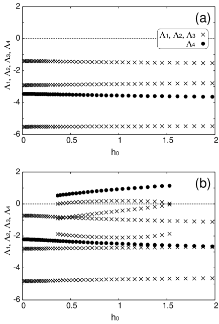
Figure 2: The dependence of the real parts of the eigenvalues of Eq. (32) on the field amplitude $h_{0}$: (a) $k=1.0$ and (b) $k=0.83$.

The dependence of the real parts of the eigenvalues on the field amplitude $h_{0}$ is shown in Fig. 2. Here, we take the values of the parameters, $\alpha$, $\beta$, and $\gamma$, used in Fig. 1. For $k=1.0$, all the real parts of the eigenvalues ($\Lambda_{1},\ldots,\Lambda_{4}$) are always negative. In other words, the SPs are stable and a traveling pattern cannot appear. For $k=0.83$, however, extra SPs appear in the region between $h_{0}\simeq 0.35$ and $h_{0}\simeq 1.5$. In that region, $\Lambda_{4}$ and one of the other three ($\Lambda_{1},\Lambda_{2},\Lambda_{3}$) are positive. Incidentally, it is confirmed that $A_{0}+\rho_{0}\sin\delta\neq 0$ in the region. This result suggests that a traveling pattern can appear in a certain region of the field when $k=0.83$.

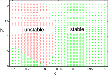
Figure 3: Stability diagram in $k$-$h_{0}$ space. In the unstable area (red-circle points), a traveling pattern can appear. In the stable area (green-cross points), the pattern cannot travel.

Using the above analysis, we show a stability diagram in Fig. 3. In the unstable area, where there is a branch with positive $\Lambda_{4}$, a traveling pattern can appear. In the stable area, where all the branches of $\Lambda_{4}$ have negative values, it cannot appear. The values of the parameters $\alpha$, $\beta$, and $\gamma$ are the same as ones in Fig. 1. The characteristic wave number $k_{0}$ depends on the ratio of $\beta$ and $\gamma$ (see Ref. kudoS for details), and $k_{0}=1$ in our case. Though it is expected that $k\simeq k_{0}$, the actual characteristic length in the simulations is larger than $2\pi/k_{0}$. In other words, $k<k_{0}$ in the actual numerical results, although a domain pattern with a small $k$ is not always realistic. Incidentally, the field larger than $h_{0}\simeq 1.5$ may be meaningless since domain patterns should vanish under a strong field.

IV Discussion

The results in Fig. 2 suggest that a traveling pattern can exist for $k\leq 0.83$ but not for $k=1.0$. This can be interpreted as meaning that a traveling pattern should be a little fat. In fact, the actual wave numbers of domain patterns in our numerical simulations are a little less than $k=1$, although $k=0.83$ seems too small. We can say that this fact partly supports the theoretical results given here.

We have used very simple approximations, i.e. perfect parallel-stripe structures without any distortion, to investigate the instabilities of a traveling pattern. That may be one of the reasons why the present analysis has suggested a traveling pattern with $k$ smaller than that of the numerical results. In our simulations, the traveling patterns do not have a perfect parallel-stripe structure. If more complex and better approximations are employed, the actual traveling patterns exhibited by numerical simulations may be better explained.

In experiments, the perfect parallel-stripe structure is a realistic pattern. However, as mentioned above, the condition for a traveling pattern is tight even for such a simple structure. Traveling patterns with a more complex structure can be observed in experiments and the conditions of their appearance would be more complex than the present case. In any case, it is sure that a traveling pattern cannot appear without a rapid oscillating field.

V Conclusions

We have proposed two ways to describe magnetic domain patterns moving slowly under a rapidly oscillating field. One gives a model in which rapidly oscillating terms are averaged out. The time-averaged model can explain the existence of the maximum values of the field where non-uniform domain patterns are preferable. The other gives a model which includes a phase shift as the delay of the response to the field. The phase-shifted model suggests the existence of a traveling pattern which moves very slowly compared with the time scale of the field. These two models have both merits and demerits. In other words, the approximations to be employed depend on the phenomenon under consideration. We should choose a method suitable for the analysis of the phenomenon to be investigated.

Although we have focused on a traveling pattern in this paper, these two methods are promising for applying to many other domain patterns under a rapidly oscillating field.

Appendix A Numerical simulations

The numerical procedures for time evolution are almost the same as those of Refs. kudoE ; kudoS . For time evolution, we use a semi-implicit method: The exact solutions and the second order Runge-Kutta method are used for the linear and nonlinear terms, respectively. For a better spatial resolution, a pseudo-spectral method is applied. In other words, we numerically calculate the time evolutions of Eq. (6) in Fourier space:

$$\frac{\partial\phi_{\bm{k}}}{\partial t}=\alpha[\phi-\phi^{3}]_{\bm{k}}-(\beta k^{2}+\gamma G_{\bm{k}})\phi_{\bm{k}}+h(t)\delta_{\bm{k}},$$ (34)

where $[\cdot]_{\bm{k}}$ denotes the convolution sum and $G_{\bm{k}}$ is the Fourier transform of $G({\bm{r}},0)$. Since we defined $G(\bm{r},0)\equiv 1/|\bm{r}|^{3}$,

$$G_{\bm{k}}=a_{0}-a_{1}k,$$ (35)

where $k=|\bm{k}|$ and

$$a_{0}=2\pi\int_{d}^{\infty}\frac{{\rm d}r}{r^{2}},\quad a_{1}=2\pi.$$ (36)

In the simulations, we set $d=\pi/2$, which results in $a_{0}=4$.

In Fig. 1, the parameters are given as $\alpha=2.0$, $\beta=2.0$, and $\gamma=2\beta/a_{1}=2/\pi$. The frequency and amplitude of the field are $\omega=2\pi\times 5\times 10^{-2}$ and $h_{0}=0.8$, respectively. The simulations are performed on a $128\times 128$ lattice with periodic boundary conditions. The snapshots in Fig. 1 are the domain patterns at (a) $5\times 10^{3}T$, (b) $10\times 10^{3}T$, and (c) $15\times 10^{3}T$, where $T=2\pi/\omega$. If the amplitude is larger (for example, $h_{0}=0.9$, $0.95$, etc.), we can see a traveling pattern with a different structure moves to a different direction.

References

- (1) L.D. Landau and E.M. Lifshitz, Mechanics (Pergamon, Oxford, 1960).
- (2) S. Rahav, I. Gilary, and S. Fishman, Phys. Rev. Lett. 91, 110404 (2003); Phys. Rev. A 68, 013820 (2003).
- (3) S. Rahav, E. Geva, and S. Fishman, Phys. Rev. E 71, 036210 (2005).
- (4) H. Saito and M. Ueda, Phys. Rev. Lett. 90, 040403 (2003).
- (5) F.K. Abdullaev, J.G. Caputo, R.A. Kraenkel, and B.A. Malomed, Phys. Rev. A 67, 013605 (2003).
- (6) C.N. Liu, T. Morishita, and S. Watanabe, Phys. Rev. A 75, 023604 (2007).
- (7) S. Miura, M. Mino and H. Yamazaki, J. Phys. Soc. Jpn. 70, 2821 (2001).
- (8) M. Mino, S. Miura, K. Dohi and H. Yamazaki, J. Magn. Magn. Mater. 226-230, 1530 (2001).
- (9) N. Tsukamoto, H. Fujisaka, and K. Ouchi, Prog. Theor. Phys. 161, 372 (2006).
- (10) M. Mino (private communication).
- (11) B.A. Malomed amd M.I. Tribelsky, Physica 14D, 67 (1984).
- (12) P. Coullet, R.E. Goldstein, and G.H. Gunaratne, Phys. Rev. Lett. 63, 1954 (1989).
- (13) S. Douady, S Fauve, and O. Thual, Europhys. Lett. 10, 309 (1989); S. Fauve, S Douady, and O Thual, J. Phys. II (Paris) 1, 311 (1991).
- (14) S. Fauve, S. Douady, and O. Thual, Phys. Rev. Lett. 65, 385 (1990).
- (15) C.B. Price, Phys, Rev. E 55, 6698 (1997).
- (16) J. Lega and N.H. Mendelson, Phys. Rev. E 59, 6267 (1999).
- (17) T. Okuzono and T. Ohta, Phys. Rev. E 67, 056211 (2003).
- (18) F. Sagués et al., Physica D 199, 235 (2004); D.G. Míguez, V. Peŕez-Villar, and A.P. Muñuzuri, Phys. Rev. E 71, 066217 (2005).
- (19) D. Michaelis, F.Kh. Abdullaev, S.A. Darmanyan, and F. Lederer, Phys. Rev. E 71, 056205 (2005).
- (20) A.S. Kirakosyan, F.Kh. Abdullaev, and R.M. Galimzyanov, Phys. Rev. B 65, 094411 (2002).
- (21) E.A. Jagla, Phys. Rev. E 70, 046204 (2004).
- (22) E.A. Jagla, Phys. Rev. B 72, 094406 (2005).
- (23) K. Kudo, M. Mino, and K. Nakamura, J. Phys. Soc. Jpn. 76, 013002 (2007).
- (24) K. Kudo and K. Nakamura,Phys. Rev. B 76, 054111 (2007).