Role of Particle Interactions in the Feshbach Conversion of Fermion Atoms to Bosonic Molecules

Abstract

We investigate the Feshbach conversion of fermion atomic pairs to condensed boson molecules with a microscopic model that accounts the repulsive interactions among all the particles involved. We find that the conversion efficiency is enhanced by the interaction between boson molecules while suppressed by the interactions between fermion atoms and between atom and molecule. In certain cases, the combined effect of these interactions leads to a ceiling of less than $100\%$ on the conversion efficiency even in the adiabatic limit. Our model predicts a non-monotonic dependence of the efficiency on mean atomic density. Our theory agrees well with recent experiments on ⁶Li and ⁴⁰K.

Feshbach resonance has now become a focal point of the research activities in cold atom physicsTimmermans ; Stoof ; chen ; Julienne since its first experimental realizationInouye . Among these research activities, the production of diatomic molecules from Fermi atoms with Feshbach resonance is of special interest and has attracted great attention. First, it is an interesting phenomenon by itself; second, it provides a unique experimental access to the BCS-BEC crossover physicsjin . So far, by slowly sweeping the magnetic field through the Feshbach resonance, samples of over $10^{5}$ weakly bound molecules (binding energy $\sim 10$ kHz) at temperatures of a few tens of nK have been produced from quantum degenerate Fermi gasregal ; strecker ; cubizolles .

The Feshbach conversion is a complicated process involving many fermion atoms and boson molecules in a sweeping magnetic field that crosses a resonance. The theoretical description of the conversion efficiency as a function of sweep rate, atom mass, atomic density, and temperature is still under development. The existing theories include the Landau-Zener (LZ) model of two-body molecular productionlz ; goral and its many-body extension at zero temperaturevardi1 ; vardi2 ; altman , phase-space density modelhodby , and equilibration model at finite temperatureswilliams .

In this Letter we study a microscopic model of the Feshbach conversion that accounts all the two-body interactions, which include atom-atom, molecule-molecule, and atom-molecule interactions. These interactions are ignored in previous theoretical studiesgoral ; vardi1 ; vardi2 ; altman . We find that these interactions affect strongly the Feshbach conversion efficiency: the repulsive interaction between molecules tends to enhance the conversion efficiency while the other two repulsive interactions between atoms and between atom and molecule suppress the efficiency. Combined together, these interactions can yield a ceiling of less than $100\%$ for the conversion efficiency even in the adiabatic limit of the sweeping magnetic field. This interaction-suppressed conversion efficiency is in spirit the same as the broken adiabaticity by interaction in the nonlinear LZ tunnelingwu ; nlz . In addition, our model predicts a non-monotonic dependence of the conversion efficiency on mean atomic density. Our results are compared to recent experiments with ⁶Li and ⁴⁰Kstrecker ; hodby ; they are in good agreement.

To include all particle interactions, we extend the two channel modelmodel1 ; model2 ; model3 and write the Hamiltonian as

$$H = \sum_{\mathbf{k},\sigma}\epsilon_{\mathbf{k}}a_{\mathbf{k},\sigma}^{\dagger}a_{\mathbf{k},\sigma}+\left(\gamma+\frac{\epsilon_{b}}{2}\right)b^{\dagger}b$$ (1)

$$+\frac{U_{a}}{V_{a}}\sum_{\mathbf{k},\mathbf{k^{\prime}}}a_{\mathbf{k},\uparrow}^{{\dagger}}a_{-\mathbf{k},\downarrow}^{{\dagger}}a_{-\mathbf{k^{\prime}},\downarrow}a_{\mathbf{k^{\prime}},\uparrow}$$

$$+\frac{U_{ab}}{V_{a}}\sum_{\mathbf{k},\sigma}a_{\mathbf{k},\sigma}^{\dagger}a_{\mathbf{k},\sigma}b^{\dagger}b+\frac{U_{b}}{V_{b}}b^{\dagger}b^{\dagger}bb$$

$$+\frac{gV_{b}}{V_{a}^{3/2}}\sum_{\mathbf{k}}\left(b^{\dagger}a_{-\mathbf{k},\downarrow}a_{\mathbf{k},\uparrow}+a_{\mathbf{k},\uparrow}^{\dagger}a_{-\mathbf{k},\downarrow}^{\dagger}b\right)\,.$$

Here $\epsilon_{\mathbf{k}}=\hbar^{2}k^{2}/2m_{a}$ is the kinetic energy of the atom and $\sigma=\uparrow,\downarrow$ denote the two hyperfine states of the atom. $U_{a}=\Lambda U_{0},U_{ab}=\Lambda U_{1},g=\Lambda g_{0}$, and $\gamma=\gamma_{0}-\Lambda g_{0}^{2}/U_{c}$, where $\gamma_{0}=\mu_{co}(B-B_{0})$ is the molecule energy under the linearly changing magnetic field with $B=-\alpha_{r}t$, $g_{0}=\sqrt{4\pi\hbar^{2}a_{bg}\Delta B\mu_{co}/m_{a}}$ is the atom-molecule coupling chen , $U_{0}=4\pi\hbar^{2}a_{bg}/m_{a}$ is the interaction between atoms, $U_{1}=4\pi\hbar^{2}1.2a_{bg}/m_{ab}$ is the atom-molecule scattering interaction, and $U_{b}=4\pi\hbar^{2}0.6a_{bg}/m_{b}$ is the interaction between moleculesscatter . $\Lambda\equiv(1+U_{0}/U_{c})^{-1}$ and $U_{c}^{-1}=-\sum_{k}(\exp(-k^{2}/k_{c}^{2})/2\epsilon_{k})$ with the cutoff momentum $k_{c}$ representing the inverse range of interaction model3 ; kokk ; chen1 . $B_{0}$ and $\Delta B$ are Feshbach resonance point and width, respectively. $m_{a}$ and $m_{b}=2m_{a}$ are masses for atoms and molecules, and $m_{ab}=\frac{2}{3}m_{a}$ is the reduced mass for the atom-molecule interaction.

In experiments, the molecular bosons are more tightly confined in space than the fermion atoms due to their different statistics. To reflect this, we use $V_{a}$ for the volume of fermion atoms and $V_{b}$ for bosonic molecules. We assume the zero temperature limit, consider only one bosonic mode, and ignore all possible dissipations in the system, such as the loss of atoms by three-body collision.

In current experiments, the intrinsic energy width of a Feshbach resonance is much larger than the Fermi energy $E_{F}$Diener , it is therefore reasonable to assume $\epsilon_{\mathbf{k}}=\epsilon$. This is called degenerate model in Ref.model2 ; vardi1 ; vardi2 . We introduce the following operatorsvardi1 ; vardi2 , $L_{x}=\frac{\sum_{\mathbf{k}}(a_{\mathbf{k},\uparrow}^{\dagger}a_{-\mathbf{k},\downarrow}^{\dagger}b+b^{\dagger}a_{-\mathbf{k},\downarrow}a_{\mathbf{k},\uparrow})}{(N/2)^{3/2}},L_{y}=\frac{\sum_{\mathbf{k}}(a_{\mathbf{k},\uparrow}^{\dagger}a_{-\mathbf{k},\downarrow}^{\dagger}b-b^{\dagger}a_{-\mathbf{k},\downarrow}a_{\mathbf{k},\uparrow})}{i(N/2)^{3/2}},L_{z}=\frac{\sum_{\mathbf{k},\sigma}a_{\mathbf{k},\sigma}^{\dagger}a_{\mathbf{k},\sigma}-2b^{\dagger}b}{N}$, where $N=2b^{\dagger}b+\sum_{\mathbf{k},\sigma}a_{\mathbf{k},\sigma}^{\dagger}a_{\mathbf{k},\sigma}$ is the total number of atoms. The Hamiltonian becomes $H=\frac{N}{4}\left(2\epsilon-(\gamma+\frac{\epsilon_{b}}{2})-\frac{NU_{a}}{2V_{a}}-\frac{NU_{ab}}{V_{a}}\right)L_{z}-\frac{N^{2}}{16}\left(\frac{U_{a}}{V_{a}}+\frac{2U_{ab}}{V_{a}}-\frac{U_{b}}{V_{b}}\right)\left(1-L_{z}\right)^{2}+\frac{gV_{b}}{V_{a}^{3/2}}\left(\frac{N}{2}\right)^{3/2}L_{x}$ reduce . With the commutators $[L_{z},L_{x}]=\frac{4i}{N}L_{y},[L_{z},L_{y}]=-\frac{4i}{N}L_{x},[L_{x},L_{y}]=\frac{i}{N}(1-L_{z})(1+3L_{z})+o(1/N^{2})$, we can obtain the Heisenberg equations for the system $i\hbar\frac{\mathit{d}}{\mathit{d}t}L_{l}=[L_{l},H],(l=x,y,z)$. Since all the commutators vanish in the limit of $N\rightarrow\infty$ and $N$ is large in current experiments, it is appropriate to take $L_{x}$, $L_{y}$, and $L_{z}$ as three real numbers $u,v,w$, respectively. These Heisenberg equations are then reduced to

$$du/d\tau = -\delta v-2\chi v(1-w)\,,~{}~{}~{}dw/d\tau=\sqrt{2}v\,,$$ (2)

$$dv/d\tau = \frac{3\sqrt{2}}{4}(w-1)(w+\frac{1}{3})+\delta u+2\chi u(1-w)\,,$$ (3)

where $\tau=(gV_{b}\sqrt{N}/\hbar V_{a}^{3/2})t$. Because of the identity $u^{2}+v^{2}=\frac{1}{2}(w-1)^{2}(w+1)$, with introducing the canonical variable $\theta=\arctan(v/u)$ we have a classical Hamiltonian,

$$\mathcal{H} = \delta w-\chi(1-w)^{2}+\sqrt{(w-1)^{2}(w+1)}\cos\theta.$$ (4)

The above equations show that all the experimental parameters affect the system via only two dimensionless parameters $\delta$ and $\chi$. By a trivial shift of time origin, we can set $\delta=\alpha\tau$ with

$$\frac{\alpha_{r}}{\alpha}=\frac{4\pi\hbar na_{bg}\Delta B}{m_{a}}\Lambda^{2}\frac{V_{b}^{2}}{V_{a}^{2}}\,,$$ (5)

where $n=N/V_{a}$ is the mean atomic density. The nonlinear parameter $\chi$ is given by

$$\chi=\left(2.3-\frac{0.15V_{a}}{\Lambda V_{b}}\right)\frac{V_{a}}{V_{b}}\sqrt{\frac{\pi\hbar^{2}a_{bg}n}{m_{a}\mu_{co}\Delta B}}\,.$$ (6)

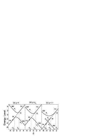
Figure 1: Adiabatic energy levels for different interaction strengths. (a)$\chi=0$; (b)$\chi=\chi_{c}=\sqrt{2}/4$; (c)$\chi=1.5$. The unstable states are indicated by dashed lines (MQ and DM).

To understand the dynamics, we first look at the fixed points $\dot{w}=\dot{u}=\dot{v}=0$ of Eqs.(2,3). The energies for these fixed points make up energy levels of the system as shown in Fig.1. One sees that the structure of these energy levels changes dramatically as the nonlinear parameter $\chi$ increases. Specifically, we observe: (i) There are two fixed points when $|\delta|$ is large enough: one for bosonic molecule (BM) and the other for fermion atom (FA). (ii) When $|\delta|<\delta_{c}=\sqrt{2}$, there is an additional fixed point with $w=1$. However, this fixed point is dynamically unstablenlz . (iii) For $\chi>\chi_{c}=\sqrt{2}/4$, there appears one more fixed point denoted by $P_{3}$ and, consequently, a loop in the energy levels. As we shall see, this loop has highly non-trivial physical consequences. This fixed point $P_{3}$ is also unstable.

Consider the adiabatic evolution of the system starting from a high negative value of $\delta$ with $w=1$. This corresponds to the experiments where the magnetic field sweeps slowly across the Feshbach resonance with no bosonic molecules initially. When $\chi$ is small, such as in Fig.1(a), the evolution of the system follows the solid line, converting all fermion atoms into molecules. However, when $\chi$ is beyond $\chi_{c}$ as in Fig.1(c), the system will find no stable energy level to follow at singular point $M$. As a result, only a fraction of fermion atoms are converted into bosonic molecules.

This simple analysis is confirmed by our numerical results, which are plotted in Fig.2. In our calculation, the 4-5th Runge-Kutta step-adaptive algorithm is used in solving the differential equations (2,3). Because $w=1$ is a fixed point when $\delta<-\sqrt{2}$, we start from $(w,u,v)\approx(1,0,0)$ and sweep the field from $\delta=-\sqrt{2}$ to $200$. In Fig.2, the conversion efficiency $\Gamma$, i.e., the fraction of the converted fermion atom pairs is drawn as a function of $\alpha$. Evidently, $\Gamma$ approaches one as $\alpha\rightarrow 0$ when $\chi<\chi_{c}$, indicating that all atomic pairs are converted into molecules. In contrast, when $\chi>\chi_{c}$, $\Gamma$ does not increase to one in the adiabatic limit $\alpha\rightarrow 0$. This means that there is a ceiling $\Gamma_{ad}$($<100\%$) on the conversion efficiency. Moreover, Fig.2 demonstrates that positive $\chi$ suppresses the conversion efficiency whereas the negative $\chi$ enhances it. Because the repulsive interaction between bosonic molecules enters $\chi$ as a negative value, it enhances the conversion efficiency; the repulsive fermion atomic interaction and atom-molecule interaction contribute positively to $\chi$, they suppress the conversion.

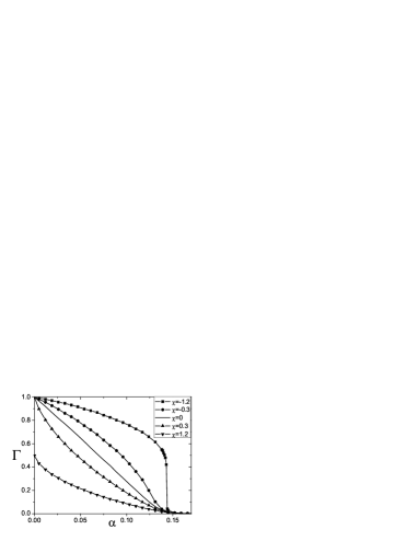
Figure 2: Conversion efficiency $\Gamma$ as a function of the sweeping rate $\alpha$ for various interactions.

The ceiling $\Gamma_{ad}$ on the atom-molecule conversion efficiency depends on $\chi$. This dependence can be found by examining the phase space diagrams of our system shown in Fig.3. As $\delta$ ramps up slowly from a large negative value, the fixed point $P_{3}$ will move up until it hits the fixed point $w=1,u=0,v=0$, represented by a dark straight line in Fig.3(a). This collision occurs at $\delta=-\sqrt{2}$. Immediately after the collision, the hyperbolic fixed point $P_{3}$ is no longer a fixed point and becomes a solution that evolves along the dark line in Fig.3(b). The dark line is given by $\sqrt{2}=\chi(1-w)-\sqrt{1+w}\cos\theta$, which is found by taking $E=\delta=-\sqrt{2}$ in the Hamiltonian (4). As the action of this trajectory is nonzero while a fixed point has zero action, this collision of the two fixed points represents a sudden jump in action. It is this sudden jump that has caused the nonzero fraction of remnant atoms. As $\delta$ ramps up further slowly, the trajectory will change its shape as witnessed in Fig.3(c); however, its action stays constant as demanded by the classical adiabatic theoremlan ; lwn . The action is

$$I=\begin{cases}\frac{1}{2\pi}\oint\frac{\cos\theta\sqrt{8\chi^{2}-4\sqrt{2}\chi+\cos^{2}\theta}}{2\chi^{2}}\mathit{d}\theta,&\frac{\sqrt{2}}{4}<\chi<\frac{\sqrt{2}}{2};\\ \frac{1}{2\pi}\int_{0}^{2\pi}\frac{4\chi^{2}-2\sqrt{2}\chi+\cos^{2}\theta}{2\chi^{2}}\mathit{d}\theta,&\chi>\frac{\sqrt{2}}{2},\end{cases}$$ (7)

which yields the ceiling on the efficiency

$$\Gamma_{ad}=1-\frac{1}{2}I=\frac{4\sqrt{2}\chi-1}{8\chi^{2}},\chi>\frac{\sqrt{2}}{4};\quad\Gamma_{ad}=1,\chi<\frac{\sqrt{2}}{4}.$$ (8)

Figure 3: Phase spaces of Hamiltonian (4). The dark line in (a) is for the fixed point $w=1,u=0,v=0$. It is a line because $\theta$ is not defined at $u=v=0$. The two fixed points on line $w=1$ in (c) are in fact the same fixed point; they are artifact caused by the definition $\theta=\arctan(v/u)$.

Now we compare our theory with existing experiments. For the experiment with ⁶Listrecker , the mean density is $n=4\times 10^{12}{\rm cm}^{-3}$ with $N=6\times 10^{5}$ atoms. The scattering length $a_{bg}=59a_{B}$, $\mu_{co}\sim 2\mu_{B}$, where $a_{B}$ and $\mu_{B}$ are Bohr radius and Bohr magneton, respectively, and the resonance width $\Delta B=0.1$G at $B_{0}=543.8$G. The Fermi energy $E_{F}$ in the combined harmonic and box-like trapping potential of Ref.strecker is given by $E_{F}=\left[15\pi N\hbar^{3}\omega_{r}^{2}/\left(8\sqrt{2m_{a}}L\right)\right]^{2/5}$, where $\omega_{r}=2\pi\times 800{\rm s}^{-1}$ is the angular frequency of the radial harmonic trap and $L=480\mu$m is the size of the axial potential. The ground state energy of molecular bosons is $E_{G}=\hbar\omega_{r}+\hbar^{2}\pi^{2}/(2m_{b}L^{2})$. Then we have $V_{a}/V_{b}=E_{F}/E_{G}=36$. We set $\Lambda=391$ with a momentum cutoff $K_{c}=96k_{F}$note . From Eq.(5), the sweeping rate is $\alpha_{r}/\alpha=20{\rm G/ms}$. The second term in the bracket of Eq.(6) that accounts for the repulsive interaction between bosonic molecules is small, so the interaction parameter takes the form of $\chi\simeq 2.3\frac{V_{a}}{V_{b}}\sqrt{\frac{\pi\hbar^{2}a_{bg}n}{m_{a}\mu_{co}\Delta B}}$. From the above experimental parameters, we find the interaction parameter as $\chi=1.26$. This strong interaction ($>\chi_{c}$) indicates a ceiling of $\Gamma_{ad}=0.48$ via Eq.(8). This is in good agreement with experiments (see Fig.4a).

For ${}^{40}{\rm K}$, the situation is different. The resonance at $B_{0}=202.1$G has a large width of $\Delta B=7.8$G and the mass of ⁴⁰K is 7 times that of ⁶Li. In Ref.hodby , the fermions are confined in a dipole trap characterized by a radial frequencies $\nu_{r}$ between 312 and 630 Hz and an aspect ratio of $\nu_{r}/\nu_{z}=70$. The Fermi energy is $E_{F}=\hbar\left(3N\omega_{r}^{2}\omega_{z}\right)^{1/3}$ and the ground state energy of condensed bosons is $E_{G}=\hbar\omega_{r}+\hbar\omega_{z}/2$. For the dipole trap, the ratio $V_{a}/V_{b}=\left(E_{F}/E_{G}\right)^{3/2}=251$. With $a_{bg}=174a_{B}$, $\mu_{co}\sim 2\mu_{B}$, initial clouds have mean densities $n=2\times 10^{12}$cm^-3, and $N=2.5\times 10^{5}$hodby , we obtain $\chi=0.135\sim 0.274$, which is less than the threshold $\chi_{c}=\sqrt{2}/4$. Therefore, ${}^{40}{\rm K}$ atom pairs can be completely converted to bosonic molecules in adiabatic limit. Indeed, the conversion efficiency up to $90\%$ has been observedhodby .

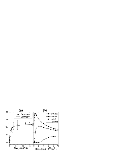
Figure 4: (a)Comparison between our theory and experimental data of ⁶Listrecker for the conversion efficiency $\Gamma$ as a function of field sweep rates. (b) The dependence of $\Gamma$ on the mean atomic density.

We emphasize that the suppressed conversion efficiency by particle interaction dominates only at low temperatures. As a result, in the above we have only compared to the data obtained at low temperatures ($T/T_{F}=0.1$ for ⁶Li and $T/T_{F}=0.05$ for ${}^{40}{K}$). Temperature can affect the conversion efficiency strongly as reported in Ref. hodby . The ceiling of $50\%$ conversion efficiency observed in Ref.regal is likely a thermal effect since the experiment is performed at $T/T_{F}=0.33$, and has been explained by the theories of finite temperaturepazy ; Chwe

For the ⁶Li, from Eq.(2)(3)we have also calculated numerically the conversion efficiency as a function of sweeping rate. The comparison between our theory and experiment is shown in Fig.4a. They are in a good agreement. In addition, our model predicts a non-monotonic dependence of the conversion rate on the mean atomic density (see Fig.4(b)). This can be understood from Eqs.(5,6). In Eq.(5), we see the effective sweeping rate $\alpha$ is inversely proportional to the atomic density. So, increasing the density will reduce the effective sweeping rate and therefore enhance the conversion rate. On the other hand, higher density will give larger nonlinearity $\chi$ as indicated in Eq.(6), which in turn suppresses the atom-molecule conversion. These two factors compete with each other, giving rise to the non-monotonic curves in Fig.4(b). In practical experiments, to achieve higher conversion efficiency, one needs to carefully choose initial fermion atom density, making it fall into the optimal parameter regime.

In summary, we have identified the significant role of the interactions between particles in the Feshbach conversion of atomic fermion pairs to molecular bosons. Our theory is consistent with the existing experiments. Our model also predicts a non-monotonic dependence of the conversion rate on the mean atomic density, which is important for the optimal choice of parameters in future Feshbach experiments.

This work was supported by NSF of China (10725521,10604009,10504040) and the 973 project (2006CB921400,2007CB814800). B.W. is also supported by the “BaiRen” program of the CAS.

References

- (1) E. Timmermans, P. Tommasini, M. Hussein, and A. Kerman, Phys. Rep. 315, 199 (1999).
- (2) R.A. Duine and H.T.C. Stoof, Phys. Rep. 396, 115 (2004).
- (3) Q. Chen, J. Stajic, S.N. Tan, and K. Levin, Phys. Rep. 412, 1 (2005).
- (4) T. Köhler, K. Góral, and P.S. Julienne, Rev. Mod. Phys. 78, 1311 (2006).
- (5) S. Inouye et al., Nature 392, 151 (1998).
- (6) C.A. Regal, M. Greiner, and D.S. Jin, Phys. Rev. Lett. 92, 040403 (2004).
- (7) C.A. Regal et al., Nature (London) 424, 47 (2003).
- (8) K.E. Strecker, G.B. Partridge, and R.G. Hulet, Phys. Rev. Lett. 91, 080406 (2003).
- (9) J. Cubizolles et al., Phys. Rev. Lett. 91, 240401 (2003).
- (10) C. Zener, Proc. R. Soc. A137, 696 (1932); L.D. Landau and E.M. Lifshitz, Quantum Mechanics (Pergamon, Oxford, 1977).
- (11) K. Goral et al., J. Phys. B 37,3457 (2004).
- (12) E. Pazy et al., Phys. Rev. Lett. 95, 170403 (2005).
- (13) I. Tikhonenkov et al., Phys. Rev. A. 73, 043605 (2006).
- (14) E. Altman and A. Vishwanath, Phys. Rev. Lett. 95, 110404 (2005).
- (15) E. Hodby et al., Phys. Rev. Lett, 94, 120402 (2005).
- (16) J.E. Williams et al, J. Phys. B, 37 (2004) L351-L357
- (17) B. Wu and Q. Niu, Phys. Rev. A 61, 023402 (2000).
- (18) J. Liu et al., Phys. Rev. A 66, 023404 (2002).
- (19) J. Javanainen et al., Phys. Rev. Lett. 92, 200402 (2004); R. A. Barankov and L. S. Levitov, ibid. 93, 130403 (2004); A. V. Andreev et al., ibid. 93, 130402 (2004); J. Dukelsky et al., ibid. 93, 050403 (2004).
- (20) T. Miyakawa and P. Meystre, Phys. Rev. A 71, 033624 (2005).
- (21) W. Yi and L.-M.Duan, Phys. Rev. A 73, 063607 (2006).
- (22) Here the of atom-molecule and molecule-molecule is taken to be 1.2 and 0.6 times that of atom-atom, respectively, see D. S. Petrov, C. Salomon, and G. V. Shlyapnikov, Phys. Rev. Lett. 93. 090404 (2004).
- (23) S. J. J. M. F. Kokkelmans et al., Phys. Rev. A 65, 053617 (2002).
- (24) Q. Chen and K. Levin, Phys. Rev. Lett. 95, 260406 (2005).
- (25) R.B. Diener and T.-L. Ho, cond-mat/0405174.
- (26) In deducing the atom-atom scattering term we need introduce the collective pseudo-spin operators . It is easy to prove that is a conservation and . Combining the conserved relation of the total paticles, , we can rewrite the atom-atom scattering term as .
- (27) L.D. Landau and E.M. Lifshitz, Mechanics (Pergamon, Oxford, 1977).
- (28) J. Liu, B. Wu, and Q. Niu, Phys. Rev. Lett. 90, 170404 (2003)
- (29) The cutoff is chosen such that the tunnelling window for converting atomic fermions to molecular bosons is consistent with the Feshbach resonance width of 6Li.
- (30) E. Pazy, A. Vardi, and Y. B. Band, Phys. Rev. Lett. 93, 120409 (2004).
- (31) J. Chwedeńczuk, K. Góral, T. Köhler, and P. S. Julienne, Phys. Rev. Lett. 93, 260403 (2004).