Gauge symmetry in Kitaev-type spin models and index theorems on odd manifolds

Abstract

We construct an exactly soluble spin-$\frac{1}{2}$ model on a honeycomb lattice, which is a generalization of Kitaev model. The topological phases of the system are analyzed by study of the ground state sector of this model, the vortex-free states. Basically, there are two phases, A phase and B phase. The behaviors of both A and B phases may be studied by mapping the ground state sector into a general $p$-wave paired states of spinless fermions with tunable pairing parameters on a square lattice. In this $p$-wave paired state theory, the A phase is shown to be the strong paired phase, an insulating phase. The B phase may be either gapped or gapless determined by the generalized inversion symmetry is broken or not. The gapped B is the weak pairing phase described by either the Moore-Read Pfaffian state of the spinless fermions or anti-Pfaffian state of holes depending on the sign of the next nearest neighbor hopping amplitude. A phase transition between Pfaffian and anti-Pfaffian states are found in the gapped B phase. Furthermore, we show that there is a hidden SU(2) gauge symmetry in our model. In the gapped B phase, the ground state has a non-trivial topological number, the spectral first Chern number or the chiral central charge, which reflects the chiral anomaly of the edge state. We proved that the topological number is identified to the reduced eta-invariant and this anomaly may be cancelled by a bulk Wess-Zumino term of SO(3) group through an index theorem in 2+1 dimensions.

I Introduction

The concept of the topological order recently is widely interesting the condensed matter physicists because it may describe the different ’phases’ without breaking any global continuous symmetry of the system wenniu . However, unlike the conventional order related to the symmetry of the system in Landau’s phase transition theory, the topological order of quantum states is not well defined yet. For example, in the quantum Hall effects, the topological property of the quantum stats may be reflected by the filling factor of the Landau level which may be thought as a topological index, the first Chern number in magnetic Brilliouin zone ttnn ; niu . Nevertheless, only the first Chern number can not fully score the topological order of the quantum Hall states. In a given filling factor, the quasiparticles may obey either abelian or non-abelian statistics. On the other hand, the edge state may partially image the topological properties of the bulk state wen . In quantum Hall system, it was seen that the edge state may be described by a conformal field theory mr . Thus, according to the bulk-edge correspondence due to the gauge invariance, it shows that the bulk state is determined by a Chern-Simons topological field theory cs . However, the bridge between the microscopic theory of the two-dimensional electron gas and the Chern-Simons theory was not spanned.

Kitaev recently constructed an exactly soluble spin model in a honeycomb lattice ki . Using a Majorana fermion representation, he found the quantum state space is characterized by two different topological phases even there is not any global symmetry breaking. The A phase is a gapped phase which has a zero spectral Chern number and the vortex excitations obey abelian anyonic statistics. The B phase is gapless at special points of Brilliouin zone. When the B phase is gapped by a perturbation, it is topologically non-trivial and has an odd-integer spectral Chern number. (We call the gapless B phase the B1 phase and gapped one the B2 phase.) Kitaev showed that if the spectral Chern number is odd, there must be unpaired Majorana fermions and then the vortex excitations obey non-abelian statistics. Consistent with the non-abelian statistics, the fusion rules of the superselection sectors of Kitaev model are the same as those of the Ising model. However, the source of the non-abelian physics has not been clearly revealed yet. On the other hand, the first Chern number can only relate to an abelian group and therefore, an odd spectral Chern number leads to a non-abelian physics but an even one did not is topologically hard to be understood.

Although Kitaev model has a very special spin coupling, its very attractive properties caused a bunch of recent studies note ; bas ; duan ; cn ; yw ; yzs ; yu ; lzx ; yk ; sdv ; lkc ; sdm ; kw . It is convenient to understand Kitaev model if one can map this model to a familiar model. In fact, Kitaev model may be mapped into a special $p$-wave paired BCS state if only the vortex-free sector of the model is considered cn . We recently generalized Kitaev model to an exactly soluble model whose vortex-free part is equivalent to $\Delta_{1x}p_{x}+\Delta_{1y}p_{y}+i(\Delta_{2x}p_{x}+\Delta_{2y}p_{y})$-wave paired fermion states with tunable pairing order parameters $\Delta_{ab}$ on a square lattice. yw . The phase diagram of our model has the same shape as that of Kitaev model, i.e, the boundary of the A-B phases are corresponding to the points ${\bf p}=(0,0),(0,\pm\pi)$ and $(\pm\pi,0)$ in the first Brilliouin zone. The A phase is gapped and may be identified as the strong paring phase of the $p$-wave paired state rg . The B phase can be either gapped or gapless even if T-symmetry is broken. We find that gapless excitations in the B phase, i.e., the B1 phase, is protected by a generalized inversion (G-inversion) symmetry under $p_{x}\leftrightarrow{\Delta_{1y}\over\Delta_{1x}}p_{y}$ and the emergence of a gapped B(B2) phase is thus tied to G-inversion symmetry breaking. For instance, the $p_{x}+ip_{y}$ wave paired state is gapped while $p_{y}+ip_{y}$-wave paired state is gapless although they both break the T-symmetry. The critical states of the A-B phase transition remains gapless whether or not T- and G-inversion symmetries are broken, indicative of its topological nature. Indeed, if all $\Delta_{ab}$ are tuned to zero, the topological A-B phase transition is from a band insulator to a free Fermi gas. The Fermi surface shrinks to a point zero at criticality.

In this paper, we further generalize the model proposed by the present author and Wang in ref. yw to a model whose square lattice mapping includes a next nearest hopping of the spinless fermions. In this case, the A phase is still a strong pairing phase as before. However, the B2 phase has more fruitful structure. The particle-hole symmetry is broken even if the chemical potential and the pairing parameters vanish. Near the long wave length limit (${\bf p}^{*}=(0,0)$ critical line), the effective chemical potential has the different sign from that of the nearest neighbor hopping amplitude. Near other two critical lines $(0,\pi)$ and $(\pi,0)$, when the next nearest neighbor amplitude is positive, the effective chemical potential is also positive. When the next nearest neighbor amplitude is negative, the effective chemical potential is also negative. A positive chemical potential corresponds to a closed Fermi surface of the particles and then a Pfaffian of the particles while a negative chemical potential to a closed Fermi surface of holes and then an anti-Pfaffian of the holes of the spinless fermion. Therefore, a Pfaffian/anti-Pfaffian phase transition happens in the B2 phase. This Pfaffian/anti-Pfaffian phase transition has been seen in the context of the $\nu=5/2$ fractional quantum Hall effect pfapf1 ; pfapf2 . The model we present here is exactly the same as a toy model on square lattice to study the Pfaffian and anti-Pfaffian physics pfapf1 . The B1 and B2 phases when the next nearest neighbor hopping is absent are corresponding to the particle-hole symmetry is conserved or spontaneously broken.

The another topic of this paper is trying to reveal the mathematical connotation behind the topological order. We emphasize that there is a hidden SU(2) gauge symmetry in this model if the model is represented by Majorana fermion operators. This non-abelian gauge symmetry is the source of the non-abelian physics of the model. The non-abelian degrees of freedom in the A phase are confined while in the B2 phase, the non-abelian degrees of freedom are deconfined. There is a Wess-Zumino(ZW) term for SU(2)/$Z_{2}$ group whose lever $k$ may character the confinement-deconfinement phases. A level $k$ WZ term corresponds to a level $k$ SU(2)/$Z_{2}$ Chern-Simons topological field theory. It was known that $k=1$ theory can only have abelian anyon while $k=2$ theory includes non-abelian anyons witten . A recently proved index theorem in 2+1 dimensions shows that the sum of this WZ term and a reduced eta-invariant $\bar{\eta}$ is an integer daizh . We show that difference between the WZ term and a part of the eta-invariant gives an ambiguity of the WZ term. Another part of this eta-invariant is identical to the chiral central charge, a half of the spectral Chern number. Thus, an odd Chern number corresponds to a $\pi i$ ambiguity while an even Chern number to a $2\pi i$ ambiguity. According to the bulk-edge correspondence, the former is consistent with $k=2$ while the latter is consistent with $k=1$.

The rest of this work was organized as follows. In Sec. II, we recall Kitaev model and show the SU(2) gauge invariance. In Sec. III, we will describe the generalized model. In Sec. IV, we give the phase diagram of the system. In Sec. V, we consider the continuous limit of our model and show that the low energy effective theory is the Majorana fermions coupled to a SO(3) gauge field in a pure gauge. In Sec. VI, we apply the index theorem on odd manifold to our model. In Sec. VII, we present a understanding to the edge state from the index theorem point of view. The section VIII is our conclusions. We arrange three appendices. Appendix A is to address the mathematic expression of the index theorem on odd manifold because most of physicists are not familiar with it. In Appendix B, we give an introduction to the representation to the spin-1/2 in the conventional fermion and Majorana fermion. And in Appendix C, for completeness, we recall the vortex excitations in our model although it was studied in our previous work yw .

II Kitaev model

We first recall some basic results of Kitaev model, which is a spin system on a honeycomb lattice ki . The Hamiltonian is given by

$$H_{ki}=-J_{x}\sum_{x{-\rm links}}\sigma^{x}_{i}\sigma^{x}_{j}-J_{y}\sum_{y{-\rm links}}\sigma^{y}_{i}\sigma^{y}_{j}-J_{z}\sum_{z{-\rm links}}\sigma^{z}_{i}\sigma^{z}_{j},$$

where $\sigma^{a}$ are Pauli matrices and ’x-,y-,z-links’ are three different links starting from a site in even sublattice ki . This model is exactly solvable if one uses a Majorana fermion representation for spin. Kitaev has shown that his Hamiltonian has a $Z_{2}$ gauge symmetry acting by a group element, e.g., for (123456) being a typical plaque

$$W_{P}=\sigma^{x}_{1}\sigma^{y}_{2}\sigma^{z}_{3}\sigma^{x}_{4}\sigma^{y}_{5}\sigma^{z}_{6}$$

with $[H_{ki},W_{P}]=0$. In fact, we can show that this model has an SU(2) gauge symmetry in the Majorana fermion representation. Let $b_{x,y,z}$ and $c$ be four kinds of Majorana fermions with $b_{x}^{2}=b_{y}^{2}=b_{z}^{2}=c^{2}=1$ and define

$$(\chi^{cd})=\frac{1}{2}\left(\begin{array}[]{cc}b_{x}-ib_{y}&b_{z}-ic\\ b_{z}+ic&-b_{x}-ib_{y}\\ \end{array}\right).$$ (1)

One observes SU(2) gauge invariant operators

$${\hat{\sigma}^{a}}=\frac{1}{2}{\rm Tr}[\chi^{\dagger}\chi(\sigma^{a})^{T}]=\frac{i}{2}(b_{a}c-\frac{1}{2}\epsilon_{abc}b_{b}b_{c})$$ (2)

with respect to the local gauge transformation $\chi^{cd}\to U^{cc^{\prime}}\chi^{c^{\prime}d}$ and then $(\chi^{\dagger})^{cd}\to(\chi^{\dagger})^{cc^{\prime}}(U^{-1})^{c^{\prime}d}$ for $U\in$SU(2) aff . It is easy to check that $\hat{\sigma}^{a}/2$ may serve as spin-1/2 operators. Replacing $\sigma^{a}$ by $\hat{\sigma}^{a}$, Kitaev model has a hidden SU(2) gauge symmetry which is trivial in the spin operator representation. The constraint $D=1$ is also gauge invariant because $D=b_{x}b_{y}b_{z}c=-i{\hat{\sigma}}^{x}{\hat{\sigma}}^{y}{\hat{\sigma}}^{z}$. Under this constraint, $\hat{\sigma}^{a}$ takes the form $ib_{a}c$ after using $b_{x}b_{y}b_{z}c=1$. The SU(2) symmetry of $\sigma^{a}=ib_{a}c$ can be directly checked

$$\sigma^{a}=ib_{a}c=ib_{a}^{\prime}c^{\prime},$$ (3)

where

$$\left(\begin{array}[]{c}b_{x}^{\prime}\\ b_{y}^{\prime}\\ b_{z}^{\prime}\\ c^{\prime}\\ \end{array}\right)=\left(\begin{array}[]{cccc}\alpha_{1}&\alpha_{2}&\beta_{1}&-\beta_{2}\\ -\alpha_{2}&\alpha_{1}&-\beta_{2}&-\beta_{1}\\ -\beta_{1}&\beta_{2}&\alpha_{1}&\alpha_{2}\\ \beta_{2}&\beta_{1}&-\alpha_{2}&\alpha_{1}\\ \end{array}\right)\left(\begin{array}[]{c}b_{x}\\ b_{y}\\ b_{z}\\ c\\ \end{array}\right)$$ (4)

with $\alpha_{1}^{2}+\alpha_{2}^{2}+\beta_{1}^{2}+\beta_{2}^{2}=1$ and $b_{x}b_{y}b_{z}c=b_{x}^{\prime}b_{y}^{\prime}b_{z}^{\prime}c^{\prime}=1$. Using Jordan-Wigner transformation, a variety of Kitaev model on a brick-wall lattice has been exactly solved note and a real space ground state wave function is explicitly shown cn . This variety should correspond to another gauge fixed theory.

After some algebras, Kitaev transferred the Hamiltonian to a free Majorana fermion one note

$$H=\frac{1}{2}\sum_{{\bf p};\mu,\nu=b,w}H({\bf p})_{\mu\nu}c_{-{\bf p},\mu}c_{{\bf p},\nu},$$ (5)

where $H(-{\bf p})=-H({\bf p})$ and $c_{{\bf q},\mu}$ are the Fourier components of a Majorana fermion operators and $\mu=b$ or $w$ refers to the even or odd position in a $z$-link ki . The ground state is vortex-free and the corresponding Hamiltonian $H_{0}({\bf p})$ is given by

$$H_{0}({\bf p})=\left(\begin{array}[]{cc}0&if({\bf p})\\ -if^{*}({\bf p})&0\\ \end{array}\right),$$ (6)

with $f({\bf p})=2(J_{x}e^{i\bf p\cdot n_{1}}+J_{y}e^{i\bf p\cdot n_{2}}+J_{z})$. Here we still follow Kitaev and choose the basis of the translation group ${\bf n}_{1,2}=(\pm 1/2,\sqrt{3}/2)$. In the next section, we will see that deforming the angle between the $x$-link and $y$-link to a rectangle will be much convenient. The eigenenergy may be obtained by diagonalizing the Hamiltonian, which is $E_{0}({\bf p})=\pm|f({\bf p})|$. The phase diagram of the model has been figured out in Fig. 1. Kitaev calls the gapped phase as A-phase and the gapless phase B phase. The A phase is topologically trivial and gapped. It is the strong-coupling limit of SU(2) like the antiferromagnetic Heisenberg model aff and can be explained as the strong paring phase in the $p$ wave sence rg . After perturbed by an external magentic field, the B phase is gapped and has a non-zero spectral Chern number and then is topologically non-trivial citeki. Without lose of generality, we consider $J_{x}=J_{y}=J_{z}=J$. The effective Hamiltonian is then given by $H_{0}({\bf p},\Delta)=(-f_{2}({\bf p}))\sigma^{x}+(-f_{1}({\bf p}))\sigma^{y}+\Delta({\bf p})\sigma^{z}$ with $\Delta(-{\bf p})=-\Delta({\bf p})$, $f_{1}=2J+4J\cos\frac{1}{2}p_{x}\cos\frac{\sqrt{3}}{2}p_{y}$ and $f_{2}=4J\cos\frac{1}{2}p_{x}\sin\frac{\sqrt{3}}{2}p_{y}$ ($f=f_{1}+if_{2}$). Assume $\psi^{\pm}({\bf p})$ to be the solutions of Schrodinger equation $H_{0}({\bf p},\Delta)\psi^{\pm}({\bf p})=\pm E({\bf p})\psi^{\pm}({\bf p})$ with $E({\bf p})=\sqrt{|f|^{2}+|\Delta|^{2}}$. After normalization, we have ${\bf L}\cdot{\vec{\sigma}}\psi^{\pm}=\pm\psi^{\pm}$ with

$${\bf L}=\frac{1}{\sqrt{3}JE({\bf p})}(-{f_{2}}({\bf p}),-{f_{1}}({\bf p}),{\Delta}({\bf p})).$$ (7)

Explicitly, near ${\bf p}={\bf p}_{*}=-\frac{2}{3}{\bf p}_{1}+\frac{2}{3}{\bf p}_{2}$mod$({\bf p}_{1},{\bf p}_{2})$ with ${\bf p}_{1}$ and ${\bf p}_{2}$ the dual vectors of ${\bf n}_{1}$ and ${\bf n}_{2}$, it is ${\bf L}=\frac{1}{\hat{E}({\bf p})}(\delta p_{y},\delta p_{x},\frac{\Delta({\bf p}_{*})}{\sqrt{3}J})\equiv(\delta\hat{p}_{y},\delta\hat{q}_{x},\hat{\Delta})$ with $\hat{E}({\bf p})=\sqrt{(\delta p_{x})^{2}+(\delta p_{y})^{2}+\Delta^{2}/3J^{2}}$. Near ${\bf p}=-{\bf p}_{*}$, it is ${\bf L}=(\delta\hat{p}_{y},-\delta\hat{p}_{x},-\hat{\Delta}).$ According to Kitaev, one can define a spectrum Chern number by using the vector field ${\bf L}$. We will be back to this issue when studying the index theorem.

Figure 1: Phase diagram in $(J_{x},J_{y},J_{z})$-space.

This is a (1,1,1)-cross section in all positive region.

III Generalized exactly soluble model

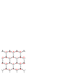
Figure 2: (Color online): The honeycomb lattices and links.

We now consider the Hamiltonian which is generalization of the Kitaev model in honeyconmb lattice to the following one

$$H = -J_{x}\sum_{x-links}\sigma_{i}^{x}\sigma_{j}^{x}-J_{y}\sum_{y-links}\sigma_{i}^{y}\sigma_{j}^{y}-J_{z}\sum_{z-links}\sigma_{i}^{z}\sigma_{j}^{z}$$

$$- \kappa_{x}\sum_{b}\sigma^{z}_{b}\sigma^{y}_{b+e_{z}}\sigma^{x}_{b+e_{z}+e_{x}}$$

$$- \kappa_{x}\sum_{w}\sigma^{x}_{w}\sigma^{y}_{w+e_{x}}\sigma^{z}_{w+e_{x}+e_{z}}$$

$$- \kappa_{y}\sum_{b}\sigma^{z}_{b}\sigma^{x}_{b+e_{z}}\sigma^{y}_{b+e_{z}+e_{y}}$$

$$- \kappa_{y}\sum_{w}\sigma^{y}_{w}\sigma^{x}_{w+e_{y}}\sigma^{z}_{w+e_{y}+e_{z}}$$

$$- \lambda_{x}\sum_{b}\sigma_{b}^{z}\sigma^{y}_{b+e_{z}}\sigma_{b+e_{z}+e_{x}}^{y}\sigma^{z}_{b+e_{z}+e_{x}+e_{z}}$$

$$- \lambda_{y}\sum_{b}\sigma_{b}^{z}\sigma^{x}_{b+e_{z}}\sigma_{b+e_{z}+e_{y}}^{x}\sigma^{z}_{b+e_{z}+e_{y}+e_{z}}$$

$$- B_{b}\sum_{b}\sigma^{z}_{b}\sigma^{y}_{b+e_{z}}\sigma^{z}_{b+e_{z}+e_{x}}\sigma^{y}_{b+e_{z}+e_{x}-e_{y}}$$

$$- B_{w}\sum_{w}\sigma_{w}^{x}\sigma_{w+e_{x}}^{z}\sigma_{w+e_{x}-e_{y}}^{x}\sigma_{w+e_{x}-e_{y}-e_{z}}^{z}$$

$$- B_{w}\sum_{b}\sigma_{b-e_{y}}^{y}\sigma_{b}^{x}\sigma_{b+e_{z}}^{y}\sigma_{b+e_{z}-e_{x}}^{x}$$

$$- B_{b}\sum_{b}\sigma^{z}_{b-e_{y}-e_{z}}\sigma^{x}_{b-e_{y}}\sigma^{x}_{b}\sigma^{y}_{b+e_{z}}\sigma^{y}_{b+e_{z}+e_{x}}\sigma^{z}_{b+e_{z}+e_{x}+e_{z}}$$

where ${}^{\prime}w^{\prime}$ and ${}^{\prime}b^{\prime}$ labels the white and black sites in lattice and $e_{x},e_{y},e_{z}$ are the positive unit vectors, which are defined as, e.g., $e_{12}=e_{z},e_{23}=e_{x},e_{61}=e_{y}$ (See Fig. 2). $J_{x,y,z}$, $\kappa_{x,y}$, $\lambda_{x,y}$ and $B_{b,w}$ are real parameters. This is a generalization of Kitaev model with the three-spin,four-spin and six-spin terms. It is easy to check this generalized Hamiltonian still has a $Z_{2}$ gauge symmetry acting by a group element, e.g., $W_{P}=\sigma^{x}_{1}\sigma^{y}_{2}\sigma^{z}_{3}\sigma^{x}_{4}\sigma^{y}_{5}\sigma^{z}_{6}$ with $[H,W_{P}]=0$. In fact, one can add more $Z_{2}$ gauge invariant multi-spin terms, e.g.,

$$\sigma_{9}^{z}\sigma_{10}^{y}\sigma^{y}_{1}\sigma^{y}_{2}\sigma^{x}_{3},$$

$$\sigma_{9}^{z}\sigma_{10}^{y}\sigma^{y}_{1}\sigma^{y}_{2}\sigma^{z}_{3}\sigma^{y}_{4},$$

$$\sigma_{9}^{z}\sigma_{10}^{y}\sigma^{y}_{1}\sigma^{y}_{2}\sigma^{y}_{3}\sigma^{z}_{16},$$

and so on. The site indices are shown in Fig. 2. For our purpose, however, we restrict on (III).

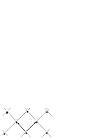
Figure 3: The effective square lattice.

We now use the Majorana fermion representation for this spin model and then the Hamiltonian reads

$$H = i\sum_{a}\sum_{a-links}J_{a}u^{a}_{ij}c_{i}c_{j}-i\sum_{b}K^{x}_{b,b+e_{z}}c_{b}c_{b+e_{z}+e_{x}}$$ (9)

$$- i\sum_{w}K^{x}_{w+e_{x}-e_{x},w-e_{z}-e_{x}}c_{w+e_{x}-e_{x}}c_{w-e_{z}-e_{x}}$$

$$- i\sum_{b}\Lambda^{x}_{b,b+2e_{z}+e_{x}}c_{b}c_{b+2e_{z}+e_{x}}$$

$$- i\sum_{w}\Lambda^{x}_{w,w-2e_{z}-e_{x}}c_{w}c_{w-2e_{z}-e_{x}}$$

$$+ y{\rm-partners}$$

$$+ i\sum_{b}\beta_{b,b+e_{z}+e_{x}-e_{y}}c_{b}c_{b+e_{z}+e_{x}-e_{y}}$$

$$+ i\sum_{w}\alpha_{w,w+e_{x}-e_{y}-e_{z}}c_{w}c_{w+e_{x}-e_{y}-e_{z}}$$

$$+ i\sum_{w}\alpha_{w,b+e_{y}+e_{x}}c_{w}c_{b+e_{y}+e_{x}}$$

$$+ i\sum_{b}\beta_{b,b+e_{z}+e_{y}+e_{x}+e_{z}}c_{b}c_{b+e_{z}+e_{x}+e_{y}+e_{z}}$$

where $K^{x}_{b,b+e_{z}}=\kappa_{x}u^{z}_{b,b+e_{z}}u^{x}_{b+e_{z}+e_{x},b+e_{z}},~{}\Lambda^{x}_{b,b+2e_{z}+e_{x}}=\lambda_{x}u^{z}_{b,b+e_{z}}u^{x}_{b+e_{z},b+e_{z}+e_{x}}u^{z}_{b+e_{z}+e_{x},b+e_{z}+e_{x}+e_{z}}$ etc and $u^{a}_{ij}=ib_{i}^{a}b_{j}^{a}$ on $a$-links. $\beta_{b,b+e_{z}+e_{x}-e_{y}}=B_{b}u^{z}_{b,b+e_{z}}u_{b+e_{z},b+e_{z}+e_{x}}^{x}u_{b+e_{z}+e_{x},b+e_{z}+e_{x}-e_{y}}^{y}$ and $\alpha_{w,w+e_{x}-e_{y}-e_{z}}=B_{w}u^{x}_{w,w+e_{x}}u_{w+e_{x},w+e_{x}-e_{y}}^{y}$ $u_{w+e_{x}-e_{y},w+e_{x}-e_{y}-e_{z}}^{z}$ etc. It can be shown that the Hamiltonian commutes with $u^{a}_{ij}$ and thus the eigenvalues of $u_{ij}=\pm 1$. Since the four spin and six-spin terms we introduced are related to the hopping between the ’b’ and ’w’ sites, Lieb’s theorem lieb is still applied. Following Kitaev, we take $u_{bw}=-u_{wb}=1$ and the vortex-free Hamiltonian is given by

$$H_{0} = i\tilde{J}_{x}\sum_{s}(c_{sb}c_{s-e_{x},w}-c_{s,w}c_{s-e_{x},b})$$

$$+ i\tilde{\lambda}_{x}\sum_{s}(c_{s,b}c_{s-e_{x},w}+c_{s,w}c_{s-e_{x},b})$$

$$+ i\frac{\kappa^{x}}{2}\sum_{s}(c_{s,b}c_{s+e_{x},b}+c_{s,w}c_{s-e_{x},w})$$

$$+ y~{}{\rm partners}+iJ_{z}\sum_{s}c_{sb}c_{sw}$$

$$+ iB_{b}\sum_{s}c_{s,b}c_{s+e_{x}-e_{y},w}+iB_{w}\sum_{s}c_{s,w}c_{s+e_{x}-e_{y},b}$$

$$+ iB_{w}\sum_{s}c_{s,w}c_{s+e_{y}+e_{x},b}+iB_{b}\sum_{s}c_{s,b}c_{s+e_{x}+e_{y},w}$$

$$= i\tilde{J}_{x}\sum_{s}(c_{sb}c_{s-e_{x},w}-c_{s,w}c_{s-e_{x},b})$$

$$+ i\tilde{\lambda}_{x}\sum_{s}(c_{s,b}c_{s-e_{x},w}+c_{s,w}c_{s-e_{x},b})$$

$$+ i\frac{\kappa^{x}}{2}\sum_{s}(c_{s,b}c_{s+e_{x},b}+c_{s,w}c_{s-e_{x},w})$$

$$+ y~{}{\rm partners}+iJ_{z}\sum_{s}c_{sb}c_{sw}$$

$$+ iB^{-}\sum_{s}(c_{s,b}c_{s+e_{x}-e_{y},w}-c_{s,w}c_{s+e_{x}-e_{y},b})$$

$$+ iB^{+}\sum_{s}(c_{s,b}c_{s+e_{x}-e_{y},w}+c_{s,w}c_{s+e_{x}-e_{y},b})$$

$$+ iB^{-}\sum_{s}(c_{s,b}c_{s+e_{x}+e_{y},w}-c_{s,w}c_{s+e_{x}+e_{y},b})$$

$$+ iB^{+}\sum_{s}(c_{s,b}c_{s+e_{x}+e_{y},w}+c_{s,w}c_{s+e_{x}+e_{y},b})$$

where $s$ represents the position of a $z$-link, $\tilde{\lambda}_{\alpha}=\frac{J_{\alpha}+\lambda_{\alpha}}{2}$ and $\tilde{J}_{\alpha}=\frac{J_{\alpha}-\lambda_{\alpha}}{2}$. $B^{\pm}=\frac{B_{b}\pm B_{w}}{2}$.

To simplify the pairing, one takes $B^{+}=0$ and denotes $B\equiv B^{-}$. Defining a fermion on $z$-links by cn ; yw

$$d_{s}=(c_{s,b}+ic_{s,w})/2,~{}~{}~{}d^{\dagger}_{s}=(c_{s,b}-ic_{s,w})/2,$$ (11)

the vortex-free Hamiltonian becomes an effective model of spinless fermions on a square lattice (Fig.3)

$$H_{0} = J_{z}\sum_{s}(d_{s}^{\dagger}d_{s}-1/2)$$ (12)

$$+ B\sum_{s}(d_{s}^{\dagger}d_{s\pm e_{x}\pm e_{y}}-d_{s}d^{\dagger}_{s\pm e_{x}\pm e_{y}})$$

$$+ \tilde{J}_{x}(d^{\dagger}_{s}d_{s+e_{x}}-d_{s}d_{s+e_{x}}^{\dagger})$$

$$+ \tilde{\lambda}_{x}\sum_{s}(d^{\dagger}_{s+e_{x}}d^{\dagger}_{s}-d_{s+e_{x}}d_{s})$$

$$+ i\kappa_{x}\sum_{s}(d_{s}d_{s+e_{x}}+d_{s}^{\dagger}d_{s+e_{x}}^{\dagger})+y~{}{\rm partners}.$$

Or it is

$$H_{0}=\sum_{\langle ij\rangle}(-td_{i}^{\dagger}d_{j}+\Delta_{ij}d^{\dagger}_{i}d^{\dagger}_{ij}+{\rm h.c.})-\mu\sum_{i}(d_{i}^{\dagger}d_{i}-1/2)$$

$$-t^{\prime}\sum_{\langle\langle ij\rangle\rangle}(d_{i}^{\dagger}d_{j}+{\rm h.c.})+\delta\sum_{i,\pm}(d_{i}^{\dagger}d_{i\pm e_{x}}-d_{i}^{\dagger}d_{i\pm e_{y}}),$$ (13)

where $t=-\frac{\tilde{J}_{x}+\tilde{J}_{y}}{2}$, $t^{\prime}=-B$, $\mu=-J_{z}$ and $\delta=\frac{\tilde{J}_{x}-\tilde{J}_{y}}{2}$. The paring parameters are defined by $\Delta_{i,i\pm e_{x,y}}=\tilde{\lambda}_{x,y}+i\kappa_{x,y}$. The last equality in eq.(13) is the toy model Hamiltonian describing Pfaffian/anti-Pfaffian states pfapf1 . Note that the pairing free Hamiltonian is particle-hole symmetry if $\Delta_{ij}=\mu=t^{\prime}=0$. The $t^{\prime}$-term breaks the particle-hole symmetry. The $\delta$-term breaks the $\pi/2$ rotational symmetry. After Fourier transformation $d_{s}=\frac{1}{\sqrt{L}_{x}L_{y}}\sum_{\bf p}e^{i{\bf p\cdot s}}d_{\bf p}$, we have

$$H_{0} = \sum_{\bf p}\xi_{\bf p}d^{\dagger}_{\bf p}d_{\bf p}+\frac{\Delta^{1}_{\bf p}}{2}(d_{\bf p}^{\dagger}d^{\dagger}_{-{\bf p}}+d_{\bf p}d_{-{\bf p}})$$ (14)

$$+ i\frac{\Delta^{2}_{\bf p}}{2}(d_{\bf p}^{\dagger}d^{\dagger}_{-{\bf p}}-d_{\bf p}d_{-{\bf p}})$$

where the dispersion relation is

$$\xi_{\bf p}=J_{z}-\tilde{J}_{x}\cos p_{x}-\tilde{J}_{y}\cos p_{y}+2B\cos p_{x}\cos p_{y}$$ (15)

and the pairing functions are

$$\Delta^{1}_{\bf p}=\Delta_{1x}\sin p_{x}+\Delta_{1y}\sin p_{y},$$

$$\Delta^{2}_{\bf p}=\Delta_{2x}\sin p_{x}+\Delta_{2y}\sin p_{y}$$ (16)

with $\Delta_{1,x(y)}=\kappa_{x(y)}$ and $\Delta_{2,x(y)}=\tilde{\lambda}_{x(y)}$. After Bogoliubov transformation,

$$\alpha_{\bf p}=u_{\bf p}d_{\bf p}-v_{\bf p}d^{\dagger}_{-\bf p},$$

$$\alpha^{\dagger}_{\bf p}=u^{*}_{\bf p}d^{\dagger}_{\bf p}-v^{*}_{\bf p}d_{-\bf p}$$ (17)

the Hamiltonian can be diagonalized

$$H_{0}=\sum_{\bf p}E_{\bf p}\alpha^{\dagger}_{\bf p}\alpha_{\bf p}+{\rm const.}$$ (18)

and the Bogoliubov quasiparticles have the dispersion

$$E_{\bf p}=\sqrt{\xi_{\bf p}^{2}+(\Delta^{1}_{\bf p})^{2}+(\Delta^{2}_{\bf p})^{2}}.$$ (19)

The Bogoliubov-de Gennes equations are given by

$$E_{\bf p}u_{\bf p}=\xi_{\bf p}u_{\bf p}-\Delta^{*}_{\bf p}v_{\bf p},~{}~{}E_{\bf p}v_{\bf p}=-\xi_{\bf p}v_{\bf p}-\Delta_{\bf p}u_{\bf p}$$ (20)

with

$$v_{\bf p}/u_{\bf p}=-(E_{\bf p}-\xi_{\bf p})/\Delta^{*}_{\bf p},$$

$$|u_{\bf p}|^{2}=\frac{1}{2}(1+\frac{\xi_{\bf p}}{E_{\bf p}}),$$

$$|v_{\bf p}|^{2}=\frac{1}{2}(1-\frac{\xi_{\bf p}}{E_{\bf p}}).$$ (21)

IV Phase diagram

We now study the phase diagram in parameter space. The phase diagram when $t^{\prime}=0$ has been discussed in our previous work yw , which has the same shape as that in original Kitaev model (with $(J_{x},J_{y},J_{z})$ in Fig.1 substituted by $(\tilde{J}_{x},\tilde{J}_{y},J_{z})$) but the structures of the B phase are more fruitful. After including the $t^{\prime}$-term, the phase boundary is still in $(p_{x},p_{y})=(0,0),(0,\pm\pi),(\pm\pi,0),(\pm\pi,\pm\pi)$ as we know before. For the present model, it is $\tilde{J}_{z}\pm\tilde{J}_{x}\pm\tilde{J}_{y}=0$ with $\tilde{J}_{z}=J_{z}+2B$ for $(0,0),(\pm\pi,\pm\pi)$ and $J_{z}-2B$ for $(0,\pm\pi),(\pm\pi,0)$. In $(\tilde{J}_{x},\tilde{J}_{y},\tilde{J}_{z})$ space, the phase diagram are of the same shape as that of original Kitaev model (Fig. 1, $(J_{x},J_{y},J_{z})$ is replaced by $(\tilde{J}_{x},\tilde{J}_{y},\tilde{J}_{z})$ ). The A phase is a strong pairing phase. The nature of the B phase is much more intriguing. Inside the B phase, $\xi_{p}$, $\Delta_{1,{\bf p}}$ and $\Delta_{2,{\bf p}}$ can be zero individually. The gapless condition ($E_{p}=0$) requires all three to be zero at a common ${\bf p}^{*}$. This can only be achieved if (i) one of the $\Delta_{a,\bf p}=0$ or (ii) $\Delta_{1,\bf p}\propto\Delta_{2,\bf p}$. If either (i) or (ii) is true, $\xi_{\bf p}$ and $\Delta_{\bf p}$ can vanish simultaneously, i.e. $E_{p}=0$ at ${\bf p}^{*}$, and the paired state is gapless. Otherwise, the B phase is gapped. Note that contrary to conventional wisdom, T-symmetry breaking alone does not guarantee a gap opening in the B phase. The symmetry reason behind the gapless condition of the B phase becomes clear in the continuum limit where $E_{p}=0$ implies that the vortex-free Hamiltonian must be invariant, up to a constant, under the transformation $p_{x}\leftrightarrow\eta p_{y}$ and $\tilde{J}_{x}\leftrightarrow\eta^{-2}\tilde{J}_{y}$ with $\eta=\frac{\Delta_{a,y}}{\Delta_{a,x}}$ with $a=1$ or $2$ and for nonzero $\Delta$. We refer to this as a generalized inversion (G-inversion) symmetry since it reduces to the usual mirror reflection when $\eta=1$. This (projective) symmetry protects the gapless nature of fermionic excitations and may be associated with the underlying quantum order wz . Kitaev’s original model has $\Delta_{1,i}=0$, and is thus G-inversion invariant and gapless. The magnetic field perturbation ki breaks this G-inversion symmetry and the fermionic excitation becomes gapped.

The continuum limit takes place near the critical line (0,0). In this case,

$$\tilde{J}_{z}-\tilde{J}_{x}-\tilde{J}_{y}-2t^{\prime}=-\mu_{eff}-2t^{\prime}=0.$$ (22)

with $\mu_{eff}=J_{z}-\tilde{J}_{x}-\tilde{J}_{y}$. Slight inside of the B phase,

$$\mu_{eff}\gtrsim-2t^{\prime}.$$ (23)

If $t^{\prime}<0$, $\mu_{eff}$ is positive and the system is in the Pfaffian phase. If $t^{\prime}>0$,

$$\mu_{eff}\lesssim 2|t^{\prime}|$$ (24)

may be either positive or negative. $\mu_{eff}>0$ means that the electron Fermi surface is closed ($\Delta_{ij}=0$) while the hole Fermi surface is opened. This is the $d$-particle paired phase. On the other hand, $\mu_{eff}<0$ means that the electron Fermi surface is opened while the hole Fermi surface is closed. This is the $d$-hole paired phase. Thus, there is a Pfaffian/anti-Pfaffian transition as $\mu_{eff}$ is across zero.

There are other two critical lines $(0,\pi)$ and $(\pi,0)$ near which there are also gapless excitations. The critical condition is given by

$$J_{z}\mp\tilde{J}_{x}\pm\tilde{J}_{y}-2B=-\mu\mp\delta+2t^{\prime}$$

$$=2t^{\prime}-\mu_{eff}=0.$$ (25)

Inside of the B phase but near the critical lines,

$$\mu_{eff}-2t^{\prime}\gtrsim 0.$$ (26)

To satisfy this condition, $\mu_{eff}$ has to be the same sign as that of $t^{\prime}$. Therefore, if $t^{\prime}>0$, the system is in the Pfaffian state and the system is in anti-Pfaffian state if $t^{\prime}<0$.

We see that when $t^{\prime}<0$, the sign of the effective chemical near the critical line $(0,0)$ has the opposite dependence on the sign of $t^{\prime}$ to the effective chemical near other two critical lines. For $t^{\prime}>0$, the sign of the effective chemical near the critical line $(0,0)$ may change from the opposite to the same as that near other two critical lines. Hence, if $t^{\prime}\neq 0$, there must be a Pfaffian/anti-Pfaffian transition inside of the gapped B phase.

At $t^{\prime}=0$, the Pfaffian and anti-Pfaffian states are degenerate. As we have seen yw , in the gapless B phase, there are two gapless Majorana excitations at nodal points while in the gapped B phase, the particle-hole symmetry is spontaneously broken, i.e., the ground state is either Pfaffian or anti-Pfaffian. All above discussions are consistent with those in ref. pfapf1 .

V Continuous limit, Dirac equations and SO(3) gauge theory

In fact, the ground state wave function for a general $p$-wave paired state can also be calculated in the continuous limit. The BCS wave function is given by

$$|\Omega\rangle=\prod_{\bf p}|u_{\bf p}|^{1/2}\exp{(\frac{1}{2}\sum_{\bf p}g_{\bf p}d^{\dagger}_{\bf p}d^{\dagger}_{\bf-p})}|0\rangle,$$ (27)

where $g_{\bf p}=v_{\bf p}/u_{\bf p}$. For even fermion number $N$, the Pfaffian ground state wave function reads

$$\Psi({\bf r}_{1},...,{\bf r}_{1})\propto\sum_{P}{\rm sgn}P\prod_{i=1}^{N/2}g({\bf r}_{P_{2i-1}}-{\bf r}_{P_{2i}})$$ (28)

with $g_{\bf p}$ is the Fourier transform of $g({\bf r})$. For the A phase, $g_{\bf p}\propto\Delta_{\bf p}$ and the analyticity of $g_{\bf p}$ leads to $g({\bf r})\propto e^{-\mu r}$ as the same calculation in a pure $p_{x}+ip_{y}$ strong pairing state. In the B phase, if the G-chiral symmetry is broken, defining $p_{a}^{\prime}=\Delta_{ab}p_{b}$ with $a=1,2$ and $b=x,y$, $g_{\bf p}\propto\frac{1}{p_{x}^{\prime}+ip_{y}^{\prime}}$ and then $g({\bf r})=\frac{1}{x_{1}^{\prime}+ix_{2}^{\prime}}$ with $x^{\prime}_{a}=\Delta^{-1}_{ab}x_{b}$. This is a Pfaffian state with $z^{\prime}=x^{\prime}_{1}+ix_{2}^{\prime}$ and is corresponding to a weak paired gapped fermion state rg .

In the long wave length limit (small $p$ limit), we approximate $\xi_{\bf p}\approx-m=\tilde{J}_{z}-\tilde{J}_{x}-\tilde{J}_{y}$ and define $\psi(t,{\bf s})=(u(t,{\bf s}),v(t,{\bf s}))$ with $(u,v)$ the Fourier transformation of $(u_{\bf p},v_{\bf p})$. The BdG equations in the gapped B phase reads

$$e^{\mu a}\gamma_{a}\partial_{\mu}\psi+im\psi=0$$ (29)

with the vielbein $e^{\mu t}=\delta_{\mu t}$ and $e^{ij}=\Delta_{ij}$. $\gamma_{0}=\sigma^{z}$ and $\gamma_{i}=\sigma^{z}\sigma^{i}$. Furthermore, it may be generalized to a curve space with spin connection term added rg . In general, the equation of $u$ is not compatible to that of $v$ and the fermions are Dirac fermions. However, it is easy to show that for this $p$-wave paired state, $u$ and $v^{*}$ obey the same equation, i.e., the anti-particle of the quasiparticle is itself. Then the fermions are Majorana ones.

We now turn to local gauge transformation. As we have pointed out, taking $u_{ij}=1$ means the whole SU(2) gauge symmetry is fixed. If making an SU(2) gauge transformation, we will run out the vortex-free state. Keeping in the vortex-free state, the gauge transformation is confined in an SU(2)/$Z_{2}\sim$ SO(3) one. Therefore, making an SO(3) transformation,

$$\psi^{\prime}({\bf r},t)=U({\bf r},t)\psi({\bf r},t),$$ (30)

Dirac equations read

$$e^{\mu a}\gamma_{a}D_{\mu}\psi^{\prime}+im\psi^{\prime}=0,$$ (31)

where the covariant derivative $D_{\mu}=\partial_{\mu}+A_{\mu}$ with $A_{\mu}=U^{-1}\partial_{\mu}U$ with $U\in$SO(3). This gauge potential is a pure gauge with a vanishing strength $F=dA+A\wedge A=0$.

We now discuss the nature of the gapless B phase in the general model with G-inversion symmetry. In this case, $E_{\bf p}=0$ at ${\bf p}=\pm{\bf p}^{*}$ which are the solutions of $\xi_{\bf p}=0$ and, say, $\Delta_{\bf p}=\Delta_{1,{\bf p}}=0$. At ${\bf p}^{*}$, the fermion dispersions are generally given by 2D Dirac cones. However, by a continuous variation of the parameters, one can realize a dimensional reduction near the phase boundary where the effective theory is in fact a 1+1 dimensional conformal field theory in the long wave length limit. Let us consider parameters that are close to the critical line with $|\sin p_{a}^{*}|\ll|\cos p_{a}^{*}|$ where $g_{\bf q}={\rm sgn}[q_{x}\Delta_{1x}\cos p_{x}^{*}+q_{y}\Delta_{1y}\cos p_{y}^{*}]\equiv{\rm sgn}(q_{x}^{\prime})$ with ${\bf q}={\bf p}-{\bf p}^{*}$. Doing the Fourier transform, we find

$$g({\bf r}) = \int dq^{\prime}_{x}dq^{\prime}_{y}e^{iq_{x}^{\prime}x^{\prime}+iq_{y}^{\prime}y}{\rm sgn}(q_{x}^{\prime})$$ (32)

$$= \delta(y^{\prime})\int dq_{x}^{\prime}\frac{q_{x}^{\prime}}{|q_{x}^{\prime}|}\sin q_{x}^{\prime}x^{\prime}\sim\frac{\delta(y^{\prime})}{x^{\prime}}.$$

The $\delta(y)$-function indicates that the pairing in the gapless B phase has a one-dimensional character and the ground state is a one-dimensional Moore-Read Pfaffian. The BdG equations reduces to

$$i\partial_{t}u=-i\Delta_{1x}(1+i\eta)\partial_{x^{\prime}}v,~{}~{}i\partial_{t}v=i\Delta_{1x}(1-i\eta)\partial_{x^{\prime}}u,$$ (33)

with $\eta=\frac{\Delta_{1y}}{\Delta_{1x}}$. Thus, the gapless Bogoliubov quasiparticles are one-dimensional Majorana fermions. The long wave length effective theory for the gapless B phase near the phase boundary is therefore the massless Majorana fermion theory in 1+1-dimensional space-time, i.e. a $c=1/2$ conformal field theory or equivalently a two-dimensional Ising model.

VI Topological invariants and Index theorem

VI.1 Spectral Chern Number and $\eta$-invariant

We note that there is no spontaneous breaking of a continuous symmetry in the phase transition from A to B phases. Kitaev has shown that the A phase in his model is topological trivial and has zero spectral Chern number while the gapped B phase has this Chern number $\pm 1$ ki . This fact was also already realized by Read and Green in the $p_{x}+ip_{y}$ paired state. Here we follow Read and Green rg to study this topological invariant for a general $p$-wave state.

In continuous limit, ${\bf p}=(p_{x},p_{y})$ is in an Euclidean space $R^{2}$. However, there is a constraint $|u_{p}|^{2}+|v_{p}|^{2}=1$, which parameterizes a sphere $S^{2}$. As $|{\bf p}|\to\infty$, $\xi_{\bf p}\to E_{\bf p}$. Then, $v_{\bf p}\to 0$ as $|{\bf p}|\to\infty$. Therefore, we can compact $R^{2}$ as an $S^{2}$ by adding $\infty$ in which $v_{\bf p}\to 0$ to $R^{2}$. The sphere $|u_{\bf p}|^{2}+|v_{\bf p}|^{2}=1$ can also be parameterized by ${\bf n_{p}}=(\Delta^{(1)}_{\bf p},-\Delta^{(2)}_{\bf p},\xi_{\bf p})/E_{\bf p}$ because $|{\bf n_{p}}|=1$. $(u_{\bf p},v_{\bf p})$ describes a mapping from $S^{2}~{}({\bf p}\in R^{2})$ to $S^{2}$ (spinor $|{\bf n_{p}}|=1$). The winding number of the mapping is a topological invariant.The north pole is $u_{\bf p}=1,v_{\bf p}=0$ at $|{\bf p}|=\infty$ and south pole $u_{\bf p}=0,v_{\bf p}=1$ at ${\bf p=0}$. For ${\bf n_{p}}$ parametrization, ${\bf n_{0}}=(0,0,\frac{\xi_{\bf p}}{E})$ at $|{\bf p}|=\infty$ and $(0,0,\frac{\xi_{\bf p}}{E})$ at ${\bf p}=0$, either the north pole or south pole.

For strong pairing phase, we know that $u_{p}\to 1$ and $v_{p}\to 0$ as ${\bf p}\to 0$ (or equivalently, $\xi_{\bf p}>0$). This means that for arbitrary ${\bf p}$, $(u_{\bf p},v_{\bf p})$ maps $p$-sphere to the up-hemishpere and then winding number is zero. That is, the topological number is zero in the strong pairing phase.

For the weak paring phase, $u_{\bf p}\to 0$ and $v_{\bf p}\to 1$ as ${\bf p}\to 0$. This means that the winding number is not zero (at least wrapping once). For our case, it may be directly calculated and the winding number is given by

$$\nu = \frac{1}{4\pi}\int dp_{x}dp_{y}\partial_{p_{x}}{\bf n_{p}}\times\partial_{p_{y}}{\bf n_{p}}\cdot{\bf n_{p}}=1$$ (34)

Defining $P({\bf p})=\frac{1}{2}(1+{\bf n_{p}}\cdot{\vec{\sigma}})$, which is the Fourier component of the project operator to the negative spectral space of the Hamiltonian, this winding number is identified as the spectral Chern number defined by Kitaev ki

$$\nu=\frac{1}{2\pi i}\int{\rm Tr}(P_{-}(\partial_{p_{x}}P_{-}\partial_{p_{y}}P_{-}\partial_{p_{y}}P_{-}\partial_{p_{x}}P_{-})]dp_{x}dp_{y}.$$ (35)

There is a topological invariant called Atiyah-Padoti-Singer eta-invraiant aps which reflects the asymmetry of the spectrum of the Dirac operator

$$\bar{\eta}(S^{2})=\frac{1}{2}\lim_{s\to 0}\int d\lambda\rho(\lambda){\rm sgn}(\lambda)|\lambda|^{-s},$$ (36)

where $\rho(\lambda)$ is the spectral density. Transforming the variable from $\lambda$ to ${\bf p}$, the measure of the integration from $\Delta_{\bf p}$ to ${\bf q}$ includes a Jacobian determinant nie ,

$$\int d\lambda...=\frac{1}{4\pi}\int d\Delta^{(1)}_{\bf p}d\Delta^{(1)}_{\bf p}\frac{1}{E_{\bf p}}...$$

$$=\frac{1}{4\pi}\int d^{2}pJ({\bf\Delta_{p},p})\frac{1}{E_{\bf p}}...$$

$$=\frac{1}{16\pi i}\int d^{2}p{\rm Tr}[J({\bf n_{p}}\cdot{\vec{\sigma}},{\bf q})...]$$

Note that $-\frac{1}{2}{\bf n_{p}}\cdot{\vec{\sigma}}$ is the signature matrix sgn$(H({\bf p}))$of the Hamiltonian, one has

$$\bar{\eta}(S^{2}) = \frac{1}{2}\lim_{s\to 0}\int d\lambda\rho(\lambda){\rm sgn}(\lambda)|\lambda|^{-s}$$ (37)

$$= \int_{S^{2}}d{\bf p}{\rm Tr[\frac{1}{2}sgn}(H({\bf p}))\rho(\frac{1}{2}{\rm sgn}(H({\bf p})))],$$

where

$$\rho(\frac{1}{2}{\rm sgn}(H({\bf q}))) = \frac{i}{16\pi}\biggl{(}\frac{\partial{\rm sgn}(H({\bf q}))}{dq_{x}}\frac{\partial{\rm sgn}(H({\bf q}))}{dq_{y}}$$ (38)

$$- \frac{\partial{\rm sgn}(H({\bf q}))}{dq_{y}}\frac{\partial{\rm sgn}(H({\bf q}))}{dq_{x}}\biggr{)}.$$

Defining the spectral projector $I-P=P_{-}({\bf q})=\frac{1}{2}(1-{\rm sgn}H({\bf q}))$, the eta-invariant is exactly equal to one half of the spectral Chern number defined by Kitaev ki

$$\bar{\eta}(S^{2})=\frac{1}{4\pi i}\int{\rm Tr}[P_{-}({\bf q})dP_{-}({\bf q})\wedge dP_{-}({\bf q})].$$ (39)

Kitaev identifies one half of $\nu$ as the chiral central charge $c_{-}$. Our result shows that this chiral central charge is just the eta-invariant. Physically, it is easy to be understood because both $c_{-}$ and $\bar{\eta}$ reflect the anomaly of the spectrum of the system.

VI.2 Index Theorem

In the continuous limit, if the space is compacted as $S^{2}$, the 2+1 space-time is a ball $X$ with a boundary $B=S^{2}_{+}(\tau=1)\cup Y\cup S^{2}_{-}(\tau=0)$ where $S^{2}_{\pm}$ are the top and bottom halves of a sphere and $Y$ is a cylinder. Now, we can apply the index theorem (46) to this spectral problem of the Dirac operator $D_{\mu}$ in $X$ with boundary $B$ daizh . The general form of thye index theorem in an odd-dimensional manifold is briefly reviewed in Appendix A. In 2+1-dimensions, the index theorem for the Toeplitz operator reads

$${\rm Ind}~{}T_{g}=\frac{1}{24\pi^{2}}\int_{X}{\rm Tr}[(gdg^{-1})^{3}]-\bar{\eta}(B,g)+\tau_{\mu}(B,P,g)$$ (40)

where the first term is equal to $\Gamma/2\pi i$ with $\Gamma$ the WZ term. The Maslov triple index $\tau_{\mu}(B,P,g)$ is an integer kl . We do not have a physical explanation of $\tau_{\mu}(B,P,g)$ yet and it possibly relates to the central charge of the theory turaev . $\bar{\eta}$ is the reduced eta-invariant. The first term in (40) determines the bulk state topological properties and the latter two terms reflect the boundary topological properties. That the index ${\rm Ind}~{}T_{g}-\tau_{\mu}$ is an integer determines the bulk-boundary correspondence.

The WZ term $\Gamma$ is defined for the fundamental representation of SU(2) but $g$ is restricted to a subgroup SU(2)/$Z_{2}\sim$ SO(3). The reduced eta-invariant is given by

$$\bar{\eta}(B,g)=\bar{\eta}(S^{2}_{+},g_{\tau=1})+\bar{\eta}(S^{2}_{-},g_{\tau=0})$$

$$=[\bar{\eta}(S^{2}_{+},g_{\tau=1})-\bar{\eta}(S^{2}_{+},g_{\tau=0})]$$

$$~{}~{}~{}+[\bar{\eta}(S^{2}_{+},g_{\tau=0})+\bar{\eta}(S^{2}_{-},g_{\tau=0})]$$

$$\equiv\Delta\bar{\eta}(S^{2}_{+})+\bar{\eta}(S^{2},g_{\tau=0}),$$ (41)

because $\bar{\eta}(Y)=0$ for $Y$ may contract to a cycle $S^{1}$. In general, $\bar{\eta}(S^{2}_{\pm},g_{1,0})=$$\frac{1}{2}[{\rm dim(ker}D(S^{2}_{\pm},g_{1,0}))+\eta(D(S^{2}_{\pm},g_{1,0}))].$ Because of a non-zero gap, ${\rm dim(ker}D(S^{2}_{\pm}))=0$. Therefore, $\bar{\eta}(S^{2},g)=\frac{1}{2}\Delta\eta(S^{2}_{+})+\frac{1}{2}\eta(D(S^{2},g_{\tau=0})).$ The discrete eigenstates of the Dirac operator do not contribute to $\bar{\eta}$ because there is no asymmetry of the spectrum for these states. $\bar{\eta}(S^{2},g_{\tau=0})=\bar{\eta}(S^{2})$ is just the eta-invariant calculated in the previous subsection.

Now, the index theorem reads

$${\rm Ind}~{}T_{g}={\Gamma}/{2\pi i}-\nu/2-\Delta\bar{\eta}(S^{2}_{+})+\tau_{\mu}(B,P,g).$$ (42)

The integrity of ${\rm Ind}~{}T_{g}-\tau_{\mu}(B,P,g)$ requires

$$\Delta\Gamma/2\pi i\equiv{\Gamma}/{2\pi i}-\Delta\bar{\eta}(S^{2}_{+})=\nu/2~{}{\rm mod}(Z).$$ (43)

Dai and Zhang have thought $\Delta\bar{\eta}(S^{2}_{+})$ as an intrinsic form of the WZ term daizh and then $\Delta\Gamma$ is in fact an ambiguity of the WZ term . It is seen that,if $\nu$ is even, one requires $\Delta\Gamma=2\pi i\times$ integer. If $\nu$ is odd , $\Delta\Gamma/2\pi i$ is required to be a half integer. In our model, it is known that for an SO(3) group, $\Delta\Gamma=\pi i\times$integer, which is consistent with $\nu=1$. In general, the index theorem (40) gives a constraint to the WZ term. An odd $\nu$ requires an even level $k$ WZ term in the effective action and the minimal one is $k=2$. This is consistent with the non-abelian anyonic statistics of the vortex excitations. For an even $\nu$, the minimal value of $k$ is one, it is consistent with the abelian anyonic statistics.

VII Edge excitations and bulk-edge correspondence

In the previous discussion, the two-dimensional space is taken to be a tours without boundary. If we consider a two-dimensional space with edge instead of the torus, Kitaev has shown that the gapless chiral edge excitations coexist with a non-zero spectral Chern numberki . This is a general result if the bulk states are gapped. In fact, it was generally known that the eta-invariant of the Dirac operator can be related to the ground state fermion charge jak ; po ; nie . By using the continuous equation $\partial_{t}\rho+\nabla\cdot{\bf j}=0$, the eat-invariant is related to the edge current integrated along the one-dimensional edge $S$, i.e.,nie

$$\eta=2\int_{S}d{\bf s}\cdot{\bf j}~{},$$ (44)

where the factor ’2’ is different from ’1’ in (104) of Kitaev in ki because of $\frac{1}{2}$ factor in (5). Thus, a non-zero eta-invariant corresponds to a non-vanishing net edge current and then the gapless chiral edge excitations. Hence, the index theorem already explained the bulk-edge correspondence.

VIII Conclusions

We studied a generalized Kitaev model whose vortex-free sector can be mapped to a $p$-wave paired state with the next nearest neighbor hopping. The phase diagram is figured out. The property of the gapped B phase was very interesting for a Pfaffian/anti-Pfaffian phase transition was found in this phase. According to the gauge invariance of the spin-1/2 theory in the fermion representation, we found the low-lying effective theory of the model is described by Majorana fermion coupled to a gauge field. The existence of this non-dynamic gauge field enabled us to understand the mathematic connotation behind these topological orders. The edge conformal anomaly can be cancelled by the bulk WZ term in terms of the recently proved index theorem on odd manifold.

IX Acknowledgement

The author would like to thank Z. Nussinov, N. Read, X. Wan, Z. H. Wang, X.-G. Wen, T. Xiang, Y. S. Wu, K. Yang, J. W. Ye and M. Yu for useful discussions. The author is grateful to Weiping Zhang for him to explain how to understand the index theorem (46). Especially, the author greatly appreciates Ziqiang Wang for our successful cooperation in ref. yw . Part of this work is the generalization of our co-work. This work was supported in part by the national natural science foundation of China, the national program for basic research of MOST of China and a fund from CAS.

Appendix A Index theorems: Mathematical preparation

Index theorems relate the analytical index of a differential operator to the topological index of a vector bundle that the operator acts on. Atiyah and Singer (AS) proved a general form of the index theorem for even dimensional compact manifold as . It said that the analytical index of an elliptical differential operator on the vector bundle is a global topological invariant which can be expressed by the integral of local topological characters on the background manifold. A generalization of the theorem to even manifolds with boundary, so-called Atiyah-Patodi-Singer (APS) theorem aps , e.g., for a Dirac operator $D$ on a manifold $M$ with boundary $\partial M$, reads

$${\rm Ind}D=\int_{M}\hat{A}(M)+\frac{1}{2}(h[\partial M]+\eta[\partial M])+\omega(\partial M),$$ (45)

where $\hat{A}$ is the Hirzebruch $\hat{A}$-class of $M$, $h$ is the dimensions of the zero modes of the boundary Dirac operator $D_{\partial M}$ and $\eta$ is the APS eta-invariant defined by $\eta(\partial M)=\lim_{s\to 0}\sum_{\lambda\neq 0}{\rm sgn}(\lambda)|\lambda|^{-s}$ where $\lambda$ is the eigenvalue of $D_{\partial M}$. $\omega(\partial M)$ is a Chern-Simons term caused by the non-product boundary metric and physically giving anomaly in quantum field theory zumino . There are many applications of the AS and APS theorem in physics, e.g, see Refs.nie ; po ; jak . Recently, index theorems were applied to chiral $p$-wave superconductors lee and graphene stone1 .

There are partners of AS and APS theorems on odd-dimensional manifolds $X$ ($d$=odd)odd1 ; odd2 ; daizh . Again, we consider Dirac operator $D$. ${\cal L}=\sum_{\lambda}{\cal L}_{\lambda}$ is the spectrum space of $D$ where ${\cal L}_{\lambda}$ is the subspace with eigenvalue $\lambda$. $P$ is a project operator defined by $P{\cal L}={\cal L}_{+}=\sum_{\lambda\geq 0}{\cal L}_{\lambda}$. Let ${\cal L}$ trivially take its value on $C^{N}$, i.e., a state $\psi\in{\cal L}$ is extended to an $N$ vector which transforms under a group GL$(N,C)$. For Toeplitz operator $T_{g}=PgP$ on odd-dimensional manifolds $X$ with boundary $B$ in which the group element $g$ is not an identity, an index theorem is given by daizh

$${\rm Ind}~{}T_{g} = -\frac{1}{(2\pi i)^{\frac{d+1}{2}}}\int_{X}\hat{A}(R^{X}){\rm Tr}[\exp(-R^{\cal L})]{\rm ch}(g)$$ (46)

$$- \bar{\eta}[B,g]+\tau_{\mu}(B,P,g),$$

where $g\in$GL$(N,C)$ (or a subgroup like SU($N$)); $R^{X}$ and $R^{\cal L}$ are the curvatures of the background manifold $X$ and ${\cal L}$; $\bar{\eta}[B,g]$ is a reduced eta-invariant and $\tau_{\mu}$, which is an integer, is the Maslov triple index kl . We do not have a physical explanation of $\tau_{\mu}$ yet and it possibly relates to the central charge of the theory turaev . ${\rm ch}(g)$ is odd Chern character defined by

$${\rm ch}(g)=\sum_{n=0}^{\frac{d-1}{2}}\frac{n!}{(2n+1)!}{\rm Tr}[(g^{-1}dg)^{2n+1}].$$ (47)

The first term in (46) determines the bulk state topological properties and the latter two terms reflect the boundary topological properties. That the index ${\rm Ind}~{}T_{g}-\tau_{\mu}$ is an integer determines the bulk-boundary correspondence.

Appendix B Spin and Majorana fermions

In this appendix, we introduce the Majorana representation of spin-1/2 operators. Consider the Pauli matrices

$$\sigma^{x}=\left(\begin{array}[]{cc}0&1\\ 1&0\\ \end{array}\right),\sigma^{y}=\left(\begin{array}[]{cc}0&-i\\ i&0\\ \end{array}\right),\sigma^{z}=\left(\begin{array}[]{cc}1&0\\ 0&-1\\ \end{array}\right),$$ (48)

with $\sigma^{x}\sigma^{y}=i\sigma^{z}$ and so on. The spin-1/2 matrices are one-half of the Pauli matrices: ${\bf S}=\frac{\vec{\sigma}}{2}$. Casimir of SU(2) group requires ${\bf S}\cdot{\bf S}=S(S+1)=3/4$ , i.e., ${\vec{\sigma}}\cdot{\vec{\sigma}}=3$. Using the conventional fermion operators $c_{\uparrow}$ and $c_{\downarrow}$, the spin-1/2 operators can be expressed by

$$\hat{\sigma}^{x}=c^{\dagger}_{\uparrow}c_{\downarrow}+c^{\dagger}_{\downarrow}c_{\uparrow}$$

$$\hat{\sigma}^{y}=-i(c^{\dagger}_{\uparrow}c_{\downarrow}-c^{\dagger}_{\downarrow}c_{\uparrow})$$

$$\hat{\sigma}^{z}=c^{\dagger}_{\uparrow}c_{\uparrow}-c^{\dagger}_{\downarrow}c_{\downarrow}.$$ (49)

That is $\hat{\sigma}^{a}=c^{\dagger}_{s}\sigma^{a}_{ss^{\prime}}c_{s^{\prime}}$. Since $\{c,c^{\dagger}\}=1,c^{2}={c^{\dagger}}^{2}=0$, one has $\hat{\sigma}^{x}\hat{\sigma}^{y}=i\hat{\sigma}^{z}$. However, it is easy to see that

$$(\hat{\sigma}^{a})^{2}=n_{\uparrow}+n_{\downarrow}-2n_{\uparrow}n_{\downarrow}$$

. To insure the Casimir operator constraint, one requires

$$n_{\uparrow}+n_{\downarrow}=1,~{}~{}n_{\uparrow}n_{\downarrow}=0$$

These are equivalent to an SU(2) constraint

$$T^{x}=c^{\dagger}_{\uparrow}c^{\dagger}_{\downarrow}+c_{\downarrow}c_{\uparrow}=0,$$

$$T^{y}=i(c^{\dagger}_{\uparrow}c^{\dagger}_{\downarrow}-c_{\downarrow}c_{\uparrow})=0,$$

$$T^{z}=n_{\uparrow}+n_{\downarrow}-1=0$$ (50)

with $T^{x}T^{y}=iT^{z}$ and so on. It is well-known taht $\{\hat{\sigma}^{a}/2,T^{a}/2\}$ form an$SO(4)\sim SU(2)\times SU(2)/Z_{2}$ Lie algebra.

The fermion expression brings extra degrees of freedom and then there is an SU(2) gauge invariant of the spin operators. Defining

$$(\chi_{\alpha\beta})=\left(\begin{array}[]{cc}c_{\uparrow}&c_{\downarrow}\\ c^{\dagger}_{\downarrow}&-c^{\dagger}_{\uparrow}\\ \end{array}\right),$$ (51)

the spin operator may be rewritten as

$${\hat{\sigma}^{a}}=\frac{1}{2}{\rm Tr}[\chi^{\dagger}\chi(\sigma^{a})^{T}]$$ (52)

Making a gauge transformation $\chi_{\alpha\beta}\to g_{\alpha\gamma}\chi_{\gamma\beta}$ and then $\chi^{\dagger}_{\alpha\beta}\to\chi^{\dagger}_{\alpha\gamma}g^{\dagger}_{\gamma\beta}$ for $g\in$SU(2) and $g^{\dagger}=g^{-1}$, one has $\hat{\sigma}^{a}$ is gauge invariant.

Majorana fermions are related to the conventional fermion through

$$c_{\uparrow}=\frac{1}{2}(b_{x}-ib_{y}),~{}~{}c_{\downarrow}=\frac{1}{2}(b_{z}-ic)$$

$$c^{\dagger}_{\uparrow}=\frac{1}{2}(b_{x}+ib_{y}),~{}~{}c^{\dagger}_{\downarrow}=\frac{1}{2}(b_{z}+ic)$$

That is,

$$b^{x}=c_{\uparrow}^{\dagger}+c_{\uparrow},~{}b^{y}=i(c_{\uparrow}^{\dagger}-c_{\uparrow}),$$

$$b^{z}=c_{\downarrow}^{\dagger}+c_{\downarrow},~{}c=i(c_{\downarrow}^{\dagger}-c_{\downarrow}).$$

It is easy to check that

$$b_{a}^{2}=1,~{}~{}~{}c^{2}=1$$

$$b_{a}b_{b}=-b_{b}b_{a},cb_{a}=-b_{a}c$$ (53)

Therefore, using the Majorana fermions, one can express the spin operators by

$$\hat{\sigma}^{x}=\frac{i}{2}(b_{x}c-b_{y}b_{z},$$

$$\hat{\sigma}^{y}=\frac{i}{2}(b_{y}c-b_{z}b_{x}),$$

$$\hat{\sigma}^{z}=\frac{i}{2}(b_{z}c-b_{x}b_{y}).$$ (54)

Correspondingly, the constraint reads

$$T^{x}=\frac{i}{2}(b_{x}c+b_{y}b_{z})=0,$$

$$T^{y}=\frac{i}{2}(b_{y}c+b_{z}b_{x})=0,$$

$$T^{z}=\frac{i}{2}(b_{z}c+b_{x}b_{y})=0.$$ (55)

Compactly, it is $D=b_{x}b_{y}b_{z}c=1$. In an explicit gauge invariant form, $D=-i\hat{\sigma}^{x}\hat{\sigma}^{y}\hat{\sigma}^{z}=1$. Using this constraint, the spin operators are simplified as

$$\hat{\sigma}^{a}=ib_{a}c.$$ (56)

Appendix C isolated vortex excitations

The isolated vortex excitations above the Pfaffian ground state has been discussed in yw . For self-containing of the paper, we repeat the paragraph which discuss the vortex excitations. The $Z_{2}$ vortex excitation in the spin model which corresponds to setting $W_{P}=-1$ for a given plaquette. Although the Hamiltonian in the fermion representation is bilinear, it is difficult to obtain analytical solutions of the wave function with vortex excitations ki . Our strategy is to evaluate the energy of the Moore-Read mr trial wave function with two well separated half-vortices located at $w_{1}$ and $w_{2}$ shown in Fig. 4 . In the gapped B phase with $p_{x}+ip_{y}$-wave pairing,

$$\Psi(z_{1},...z_{N};w_{1},w_{2})\propto{\rm Pf}(g^{\prime}(z_{i},z_{j};w_{1},w_{2})),$$

$$g^{\prime}(z_{1},z_{2};w_{1},w_{2})\propto\frac{(z_{1}-w_{1})(z_{2}-w_{2})+(w_{1}\leftrightarrow w_{2})}{z_{1}-z_{2}}.$$

$$|w_{1},w_{2}\rangle\propto\exp\{\frac{1}{2}\sum_{{\bf r}_{1},{\bf r}_{2}}g^{\prime}(z_{1},z_{2};w_{1},w_{2})d^{\dagger}_{{\bf r}_{1}}d^{\dagger}_{{\bf r}_{2}}\}$$ (57)

Performing a Fourier transformation, we have

$$|w_{1},w_{2}\rangle\propto\exp\{\frac{1}{2}\sum_{{\bf K},{\bf k}}g^{\prime}_{k}({\bf K})d_{\bf K+k}^{\dagger}d_{\bf K-k}^{\dagger}\},$$ (58)

where ${\bf k}={\bf k}_{1}-{\bf k}_{2}$ and ${\bf K}={\bf k}_{1}+{\bf k}_{2}$ are the relative and the total momenta of the pairs and $g^{\prime}_{k}({\bf K})$ is the Fourier transform of $g^{\prime}({\bf r}_{1},{\bf r}_{2})$. One can show that, in a system with linear dimension $L$, $g^{\prime}_{k}(K=0)\sim\frac{1}{k}(1/6+i/8-(1+i)(w_{1}+w_{2})/8L+w_{1}w_{2}/L^{2})$. The Hamiltonian in the presence of the two vortices shown in Fig. 1 where the red $z$-links have $u_{bw}=-1$ and all others $u_{bw}=1$, may be written as $H=H_{0}+\delta H$. Here $H_{0}$ is the vortex-free Hamiltonian and $\delta H$ is the vortex part. The latter is expressed as a sum of (twice) the pairing and chemical potential terms in Eq. (6) over the red $z$-links extending in the $\xi$-direction (the line with $x=y$) between the vortices. By a direct calculation, one can prove that $\delta H$ has the following form

$$\langle w_{1},w_{2}|\delta H|w_{1},w_{2}\rangle$$ (59)

$$\propto\sum_{p_{\xi},p^{\prime}_{\xi}}\frac{i(e^{iw_{1}(p_{\xi}+p^{\prime}_{\xi})}-e^{iw_{2}(p_{\xi}+p^{\prime}_{\xi})})}{p_{\xi}+p^{\prime}_{\xi}}f(p_{\xi},p_{\xi}^{\prime})=0,$$

where $f(p_{\xi},p_{\xi}^{\prime})$ is an analytical function of $p_{\xi}+p^{\prime}_{\xi}$. On the other hand, one can check that since $[H_{0},\sum_{\bf K,k}g^{\prime}_{k}({\bf K}\neq 0)d_{\bf K+k}^{\dagger}d_{\bf K-k}^{\dagger}]=0$, the ${\bf K}\neq 0$ sector does not play a nontrivial role in calculating $E_{v}$. The energy of such a vortex pair is given by

$$E_{v}=\langle w_{1},w_{2}|H|w_{1},w_{2}\rangle=\langle w_{1},w_{2}|H_{0}|w_{1},w_{2}\rangle$$

$$=\sum_{\bf k}E_{\bf k}|u_{\bf k}\delta g_{\bf k}|^{2}\langle w_{1}w_{2}|d_{\bf k}d^{\dagger}_{\bf k}|w_{1}w_{2}\rangle$$

$$\sim A(w_{1},w_{2})\sum_{\bf k}(1-|g^{\prime}_{\bf k}(K=0)|^{2})E_{\bf k},$$ (60)

where $\delta g_{\bf k}=g_{\bf k}^{\prime}({\bf K}=0)-g_{\bf k}$ and $A(w_{1},w_{2})$ is a positive constant. In general, $\langle w_{1}w_{2}|d_{\bf k}d^{\dagger}_{\bf k}|w_{1}w_{2}\rangle=1-|g^{\prime}_{\bf k}(K=0)|^{2}$ is the quasihole distribution when the two vortices are located at $w_{1}$ and $w_{2}$. Thus, $E_{v}$ is indeed the energy cost to excite the vortex pair. Since $g^{\prime}_{\bf k}\sim 1/k$ and $E_{\bf k}\sim k$ for $k\to 0$, there is no infrared divergence in $E_{v}$. Therefore it costs a finite energy for such vortex pair excitations which is isolated to other states in the gapped B phase. Note that $A(w_{1},w_{2})\to 0$ as $w_{1}$ and $w_{2}\to\infty$, which corresponds to the case where the bulk of the system is sent back to the vortex-free ground state.

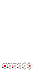
Figure 4: The vortex excitations. The grey solid circles denote $W_{P}=1$ and the red solid circles denote vortices with $W_{P}=-1$.

The finiteness of $E_{v}$ and vanishing of $\langle\delta H\rangle=0$ imply that the vortex excitations are isolate either to the ground state or the other excitations. This is consistent with analysis of Read and Green to the vortex excitations in U(1) vortex excitation of the $p$-wave paired state rg .

References

• (1) X. G. Wen and Q. Niu, Phys. Rev. B 41, 9377 (1990).
• (2) D. J. Thouless, M. Kohmoto, M. P. Nightingale, and M. den Nijs, Phys. Rev. Lett.49, 405(1982).
• (3) Q. Niu, D. J. Thouless, and Y. S. Wu, Phys. Rev. B 31, 3372(1985).
• (4) X. G. Wen, Phys. Rev. Lett. 64, 2206 (1990); Phys. Rev. B 41, 12838 (1990).
• (5) G. Moore and N. Read, Nucl. Phys. B 360, 362 (1991).
• (6) S. C. Zhang, H. Hasson, and S. Kivelson, Phys. Rev. Lett. 62 82 (1989).
• (7) A. Kitaev, Ann. Phys. 321, 2(2006).
• (8) X. Y. Feng, G. M. Zhang, and T. Xiang, Phys. Rev. Lett. 98, 087204 (2007).
• (9) G. Baskaran, S. Mandal, and R. Shankar,Phys. Rev. Lett. 98, 247201 (2007).
• (10) Y. J. Han, R. Raussendorf, and L. M. Duan Phys. Rev. Lett. 98, 150404 (2007).
• (11) H. D. Chen and J. P. Hu, arXiv:cond-mat/0702366; H. D. Chen and Z. Nussinov, arXiv:cond-mat/0703633.
• (12) Y. Yu and Z. Q. Wang, arXiv:0708.0631.
• (13) S. Yang, D. L. Zhou, and C. P. Sun, Phys. Rev. B 76, 180404 (2007).
• (14) Y. Yu, arXiv:0704.3829.
• (15) D. H. Lee, G. M. Zhang, and T. Xiang Phys. Rev. Lett. 99, 196805 (2007).
• (16) H. Yao and S. A. Kivelson, Phys. Rev. Lett. 99, 247203 (2007).
• (17) K. P. Schmidt, S. Dusuel, and J. Vidal, arXiv:0709.3017.
• (18) V. Lahtinen, G. Kells, A. Carollo, T. Stitt, J. Vala, and J. K. Pachos, arXiv:0712.1164.
• (19) K. Sengupta, D. Sen, and S. Mondal, arXiv:0710.1712.
• (20) S. P. Kou and X. G. Wen, arXiv:0711.0571.
• (21) N.Read and D.Green, Phys. Rev. B 61, 10267 (2000).
• (22) S. S. Lee, S. Ryu, C. Nayak, and M. P. A. Fisher, Phys. Rev. Lett. 99, 236807 (2007) .
• (23) M. Levin, B. Halperin, and B. Roscnow, Phys. Rev. Lett. 99, 236806 (2007).
• (24) E. Witten, Commun. Math. Phys. 121, 351 (1989).
• (25) X. Z. Dai and W. P. Zhang, J. Func. Analy. 238, 1(2006).
• (26) I. Affleck, Z. Zou, T. Hua, and P. W. Anderson, Phys. Rev. B 38, 745 (1988).
• (27) E. H. Lieb, Phys. Rev. Lett. 73, 2158 (1994).
• (28) X. G. Wen and A. Zee, Phys.Rev. B 66, 235110 (2002).
• (29) M. Niemi and G. W. Semenoff, Phys. Rep. 135, 99 (1986).
• (30) R. Jackiw, Phys. Rev. D 29, 2375 (1984).
• (31) A. P. Polychronakos, Nucl. Phys. B 278, 207 (1986); B 283, 268 (1987).
• (32) M. F. Atiyah and I. M. Singer, Ann. Math. 87, 485, 531, 546 (1968). 93 119,139 (1971).
• (33) M. F. Atiyah, V. K. Patodi, and I. M. Singer, Math. Proc. Camb. Phil. Soc. 77, 43 (1975); 78, 405 (1975); 79, 71 (1976).
• (34) B. Zumino, Y. S. Wu and A. Zee, Nucl. Phys. B 239, 477 (1984).
• (35) S. Tewari, S. Das Sarma, and Dung-Hai Lee, arXiv:cond-mat/0609556.
• (36) J. K. Pachos and M. Stone, arXiv:cond-mat/0607394.
• (37) P. Baum and R. G. Douglas, in Proc. Sympos. Pure and Appl. Math. 38,117 (1982).
• (38) R. G. Douglas and K. Wojciechowski, Commun. Math. Phys. 142, 139 (1991).
• (39) P. Kirk and M. Lesch, Forum Math. 16, 553 (2004).
• (40) V. G. Turaev, Quantum invariants of knots and 3-manifolds, de Gruyter Studies in Mathematics 18, de Gruyter (1994).