Abstract

For a quantum Hamiltonian $H=H(\lambda)$, the observability of the energies $E$ may be robust (whenever all $E$ are real at all $\lambda$) or, otherwise, conditional. Using a pseudo-Hermitian family of $N-$state chain models $H=H^{(N)}(\lambda)$ we discuss some generic properties of conditionally observable spectra.

1 Introduction

At the low energies and for the sufficiently weak interactions, quantum mechanics is a reliable theory. A transition to the full-fledged apparatus of relativistic quantum field theory is, moreover, generally believed to offer its natural extension to the higher energies and/or to the stronger interaction forces. In between these two extremes, unfortunately, there exists a huge territory of open theoretical questions. The loss of the internal consistency of many approximative phenomenological models may be encountered. Their limits of validity at certain parameters are often marked by the loss of the reality of the measurable quantities. One of the best known illustrations of such a “quantum catastrophe” is the complexification of the ground-state energy in the solvable model of a Dirac fermion moving in a overcritical external Coulomb field [1]. The same effect is encountered for the Klein-Gordon boson moving in an external scalar field [2], etc.

A particularly popular simulation of the breakdown of quantum stability has recently been found via the study of complex, ${\cal PT}-$symmetric local potentials admitting the completely real spectra [3]. Such an extension of the usual phenomenology offers multiple advantages in the context of physics (cf., e.g., its recent review [4]). At the same time, its proper implementation requires a fairly complicated mathematical apparatus [5]. This is a serious technical obstacle for any easy explanation of the parameter-controlled transitions between the real and complex energies. In fact, within the class of the ${\cal PT}-$symmetric local potentials the reality of the spectrum may prove extremely fragile [6]. For this reason one feels inclined to turn attention to the constructive study of the control of the observability of the energies (i.e., of the reality of all the eigenvalues of $H$) via some simplified models specified, say, by some finite-dimensional matrix Hamiltonians.

The first results in this direction were already obtained in our two recent remarks [7, 8] where we discussed some phenomenological aspects of certain “first nontrivial”, viz., two- and three-dimensional real-matrix models, respectively. In our present continuation of this effort we intend to extend our attention to the whole family of simplified matrix models of an arbitrary (say, even) dimension $N=2J$.

The key encouragement of such a project has been found in our computer-algebra-based paper [9] where we revealed that a transparent mathematical structure can emerge not only in the above-mentioned low-dimensional models $H^{(2)}$ and $H^{(3)}$ but also in some of their specific tridiagonal generalizations $H^{(N)}$ of any dimension $N$. For our present purposes we pick up a subset of the latter models with the even dimensions $N=2J$. The reason is pragmatic – one finds just purely formal differences between the separate even- and odd-dimensional series of the models $H^{(N)}$ of ref. [9].

Our main message will be preceded by a brief summary of the state of the art in section 2. A more detailed explanation of the problem will then follow in section 3. We emphasize there that several relevant properties of our family of the Hamiltonians may already be observed in its first, one-parametric real-matrix two-by-two member $H^{(2)}(\lambda)$. We point out the intimate connection between the parity-pseudo-Hermiticity of the model and the mechanism which makes the “observability” (i.e., the reality) of the energies lost during a smooth change of the $\lambda-$dependent matrix elements.

The next steps of our detailed analysis of chain-models $H^{(N)}(\lambda)$ are performed in sections 4 and 5 giving a detailed description of the spectra at $N=4$ and $N=6$, respectively. In section 6 some of the quantitative conclusions of this analysis are found extensible to all the dimensions $N=2J$. In particular, within the “catastrophic” loss-of-the-observability scenario we stress that the flexibility offered by the $J$ independent matrix elements in $H^{(2J)}$ suffices for the simulation and enumeration of the eligible level-confluences igniting the imminent quantum collapse.

Section 7 is a summary where we re-emphasize an exceptional suitability of our present models for deductions of some universal and generic qualitative conjectures.

2 The loss of observability in ${\cal PT}-$symmetric examples

A deep physical appeal of the ${\cal PT}-$symmetric quantum mechanics (PTSQM, [10]) lies in the variability of its definition of the inner product in the “physical” Hilbert space of states [11, 12, 13]. The idea itself is in fact not too surprising since it has been discovered, forgotten and rediscovered in field theory [14], in perturbation-theory mathematics [15, 16] as well as in nuclear physics etc [11, 17]. After its recent extremely successful popularization by Bender and Boettcher [3] its use helped to clarify also the stability of a quantum particle in many complex quantum potentials [18] – [21].

A mathematical core of the PTSQM formalism lies in its work with pseudo-Hermitian Hamiltonians $H$ such that $H^{\dagger}={\cal P}\,H\,{\cal P}^{-1}\neq H$. The intertwiner ${\cal P}$ should be an elementary operator which is, very often, identified with the parity [3, 16]. Then, the manifestly non-Hermitian Hamiltonian $H$ can only become selfadjoint (or, in the language of ref. [11], quasi-Hermitian) with respect to a nontrivial, ad hoc metric operator $\Theta\neq I$ which depends on $H=H(\lambda)$ and, hence, which can also vary with the parameter $\lambda$.

The selected $\Theta$ defines the inner product in the Hilbert space of states ${\cal H}^{(physical)}$ so that it may become singular at some “exceptional” $\lambda$ [22]. This is precisely what paved the way to the practical physical applications of the conditional reality of the eigenvalues in the single-particle relativistic context of Klein-Gordon equation [23] and of Proca equation [24] as well as in the papers on quantum anomalies [25], on supersymmetric models [26] or, beyond quantum-theory context, in cosmology [27] and in magnetohydrodynamics [28].

We believe that in virtually all of these (and many other) applications the conditional character of the reality of the eigenvalues plays the key role. For this reason let us now perform a certain systematic clarification of the related phenomenological as well as purely formal possibilities.

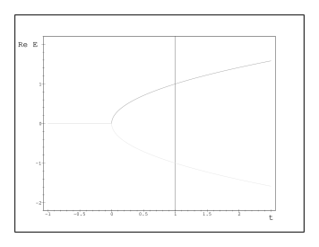
Figure 1: Real parts of the energies in the two-state model as functions of the parameter $t$.

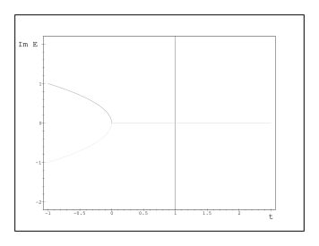
Figure 2: Imaginary parts of the energies in the two-state model as functions of the parameter $t$.

3 The loss/emergence of observability in a matrix example

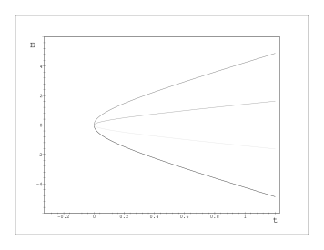
Figure 3: The four real $J=2$ energies at $A=B=1$

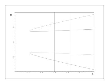
Figure 4: The four real $J=2$ energies at $A/2=B=1$

The feasibility of a controlled, conditional transition to the instability characterized by the complex eigenvalues may be understood as a direct consequence of the non-Hermitian nature of the models $H=H(\lambda)$ for which the parameter $\lambda$ either stays inside its “allowed” physical domain ${\cal D}$ or some of the energy eigenvalues $E$ become complex. Of course, the variations of $\lambda$ may be expected to depend on time. For this reason, let us change our notation and replace $\lambda$ by the more explicit symbol $t$.

Whenever our “time” $t$ reaches its critical value, the related complexification transition may be most easily visualized in the schematic two-by-two model of ref. [7],

$$H^{(2)}=\left(\begin{array}[]{cc}-1&\sqrt{1-t}\\ -\sqrt{1-t}&1\end{array}\right)\,.$$ (1)

At all $t<1$ this matrix is real and pseudo-Hermitian with respect to certain parity matrix ${\cal P}$,

$$\left[H^{(2)}\right]^{\dagger}={\cal P}H^{(2)}{\cal P}^{-1}\,,\ \ \ \ \ \ \ \ \ \ {\cal P}=\left(\begin{array}[]{cc}1&0\\ 0&-1\end{array}\right)\,.$$ (2)

The specific parametrization of its matrix elements has been chosen as giving closed formula for the two-point spectrum, $E_{\pm}^{(2)}=\pm\sqrt{t}$. Obviously, these energies generated by the Hamiltonian (1) remain complex (i.e., not observable) along all the negative half-axis, $t\in(-\infty,0)$ (cf. Figures 1 and 2). On the contrary, the matrix $H^{(2)}(t)$ becomes manifestly Hermitian (we could say, “conventionally physical”) at $t\in(1,\infty)$. In the middle, “unconventionally physical” interval of parameters $t\in(0,1)$, our non-Hermitian Hamiltonian with real energies remains, in the terminology of the review paper [11], quasi-Hermitian.

The “unconventional” choice of $t\in(0,1)$ leaves our matrix $H^{(2)}$ tractable as a valid and acceptable selfadjoint representation of an observable quantity, provided only that our Hilbert space of states ${\cal H}^{(2)}$ is properly re-defined (cf. the extensive accounts of this attitude, say, in the reviews [4, 12] or in the proceedings [29]). In this sense the message delivered by our illustrative example (1) may be read as emphasizing that even though its form may cease to be manifestly Hermitian, the operator $H$ may represent a physical observable (comment [7] may be consulted for all the technical details).

Even though the symbol $t$ represents time, let us keep both the directions of the $t-$development available. Thus, under the tacit assumption that we move to the left along the real $t-$axis in Figures (1) and (2) we speak about the confluence of the real energy levels followed by their subsequent complexification. This convention will be preferred in what follows although, alternatively, we could also change it and call the right-ward $t-$development a “big-bang-like” decomplexification of the system which stayed unobservable at the earlier times.

Our specific $t-$parametrization of the matrix elements is privileged because it mediates the smooth $t-$dependence of the eigenvalues (or of their squares at least). Thus, even when the formal Hermiticity and/or quasi-Hermiticity of the Hamiltonian $H^{(2)}$ breaks down, both the Figures 1 and 2 confirm that the $t=1$ division line between the Hermitian and non-Hermitian regime is artificial and, in any conceivable phenomenological context, irrelevant.

Our two latter comments are challenging: it is not obvious what can be expected to happen at some higher dimensions in a suitable matrix generalization of $H^{(2)}$. A few answers will be offered in what follows.

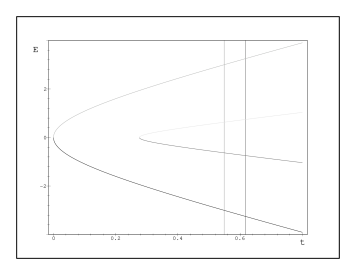
Figure 5: The four real $J=2$ energies at $A=2B/3=1$

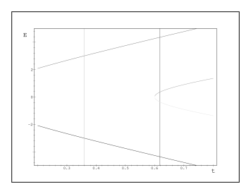
Figure 6: The four real $J=2$ energies at $A=B/5=1$

4 The first nontrivial model with four levels

The two-parametric four-by-four chain-model

$$H^{(4)}=\left(\begin{array}[]{cccc}-3&\sqrt{3-3\,\beta}&0&0\\ -\sqrt{3-3\,\beta}&-1&2\,\sqrt{1-\alpha}&0\\ 0&-2\,\sqrt{1-\alpha}&1&\sqrt{3-3\,\beta}\\ 0&0&-\sqrt{3-3\,\beta}&3\end{array}\right)\,$$ (3)

is just one of the special cases of the four-parametric pseudo-Hermitian Hamiltonians studied in ref. [30]. The quadruplet of the eigenenergies of matrix (3) is obtainable in closed form,

$$E_{\pm}=\pm\sqrt{s}\,,\ \ \ \ \ \ s=s_{\pm}=3\,\beta+2\,\alpha\pm 2\,\sqrt{3\,\beta\,\alpha+{\alpha}^{2}+9\,\beta-9\,\alpha}\,$$ (4)

so that the boundary of the two-dimensional domain ${\cal D}$ (where our pseudo-Hermitian matrix has the real spectrum) is composed of the two curves, viz.,

$$\beta\geq\beta_{minimal}=\frac{9\,\alpha-{\alpha}^{2}}{9+3\,\alpha}\,,\ \ \ \ \ \ \ \ \ \ \ \ \alpha\in(0,1)\,$$ (5)

and

$$\alpha\geq\alpha_{minimal}=\beta-\frac{\beta^{2}}{4}\,,\ \ \ \ \ \ \ \ \ \ \ \ \beta\in(0,1)\,.$$ (6)

Once we set

$$\beta=t+B\,t^{2}\,,\ \ \ \ \ \ \alpha=t+A\,t^{2}\,,$$ (7)

we may fix the auxiliary constants $A=B=1$ and stay safely inside the quasi-Hermiticity domain ${\cal D}$ at all the sufficiently small values of $t>0$. In a way illustrated by Figure 3 the $t-$dependence of the energies remains smooth also when we cross the separation point $t=t^{(GM)}=(\sqrt{5}-1)/2\approx 0.618$ between the Hermitian and non-Hermitian regimes with $t>t^{(GM)}$ and $t<t^{(GM)}$, respectively.

Once we decide to weaken the attraction between the central energies and choose, say, $A=2$ and $B=1$, the energies split in the two well-separated pairs and they remain all real whenever $t^{(QH)}>0.3104686356$, i.e., to the right from the $A-$dependent quasi-Hermiticity boundary. The resulting $t-$dependence of the spectrum is displayed in Figure 4 where the complexifications of the two different off-diagonal matrix elements are marked by the two different vertical lines. To the right of both of them, our Hamiltonian $H^{(4)}$ becomes standard and Hermitian, to the left of both of them, our matrix $H^{(4)}$ remains ${\cal P}-$pseudo-Hermitian with respect to the usual parity

$${\cal P}=\left(\begin{array}[]{cccc}1&0&0&0\\ 0&-1&0&0\\ 0&0&1&0\\ 0&0&0&-1\end{array}\right)\,.$$ (8)

Between the vertical lines, an anomalous parity matrix must be chosen to define the pseudo-Hermiticity,

$${\cal P}^{\prime}=\left(\begin{array}[]{cccc}-1&0&0&0\\ 0&1&0&0\\ 0&0&1&0\\ 0&0&0&-1\end{array}\right)\,.$$

In the complementary scenario we have to weaken the attraction between the peripheral energy levels using $B>A$. The choice of $A=1$ accompanied by the weakly enhanced $B=3/2$ leads to the result depicted in Figure 5. Due to the complexification of the most strongly attracted central pair of the levels, the quasi-Hermiticity is lost for $t<t^{(QH)}=0.2761423749$. This takes place safely below the upper boundary $t^{(SPH)}=0.5485837704$ of the pseudo-Hermitian regime specified by the standard parity operator (8). The latter feature is fragile. At the larger $B=5$ we get $t^{(SPH)}=0.3582575695$ which is perceivably smaller than the complexification bound $t^{(QH)}=3/5$ (cf. Figure 6).

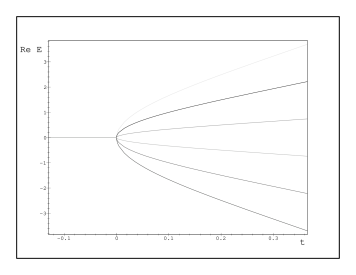
Figure 7: Real parts of the energies in the six-state model ($A=B=C=1$).

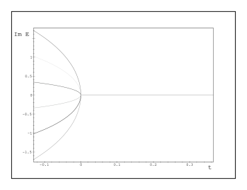
Figure 8: Imaginary parts of the energies in the six-state model ($A=B=C=1$).

5 The next, more complicated chain model with six levels

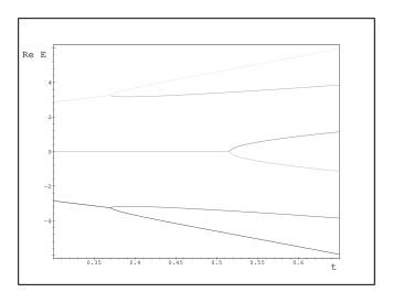
Figure 9: Real parts of the energies in the six-state model at $A=B/2=C=1$.

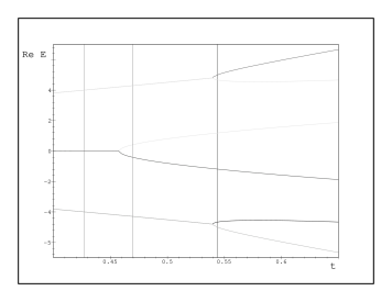
Figure 10: Real parts of the energies in the six-state model at $A/3=B/5=C=1$.

In the six-by-six model of ref. [9],

$$H^{(6)}=\left[\begin{array}[]{cccccc}-5&g_{1}&0&0&0&0\\ -g_{1}&-3&g_{2}&0&0&0\\ 0&-g_{2}&-1&g_{3}&0&0\\ 0&0&-g_{3}&1&g_{2}&0\\ 0&0&0&-g_{2}&3&g_{1}\\ 0&0&0&0&-g_{1}&5\end{array}\right]\,,$$ (9)

with

$$g_{1}=c=\sqrt{5\,(1-\gamma)}\,,\ \ \ g_{2}=b=2\,\sqrt{2\,(1-\beta)}\,,\ \ \ g_{3}=a=3\,\sqrt{1-\alpha}$$

let us set

$$\alpha=t+t^{2}+A\,t^{3}\,,\ \ \ \ \ \beta=t+t^{2}+B\,t^{3}\,,\ \ \ \ \ \gamma=t+t^{2}+C\,t^{3}\,.$$ (10)

For $A=B=C=1$ we encounter a not too interesting single pseudo-Hermiticity line $t^{(PH)}=0.5436890127$ which is, incidentally, out of the range of Figures 7 and 8. Thus, under our present interpretation of $t$ as a leftwards-running time, the choice of $A=B=C=1$ would represent a fine-tuned “big crunch” process. Let us add a comment that after a temporary reversal of our conventional arrow of time, Figure 7 mimics an even more interesting scenario of a “big-bang” development. From this point of view there exists no observable state of our schematic system at $t<0$ and just a single, fully degenerate state with $E=0$ emerges at $t=0$. Subsequently, teh evolution becomes characterized by a steady repulsion of the levels.

After we return to our leftwards-running time convention, the peripheral-weakening choice of a dominant $C$ will leave both the outermost levels far away, too weakly attracted and not sufficiently participating in the overall collapsing tendency. The first complexification will involve only the inner quadruplet of the energies. It may proceed either along the two-pair-complexification pattern indicated in Figure 4 (we choose there $A=B=C/2=1$ so that the complementary pseudo-Hermiticity boundary moved to $t^{(PH^{\prime})}=1/2$) or along the central-complexification pattern represented by Figures 5 and 6 (necessitating an increase of $B$).

The next eligible choice of dominant $A$ will weaken the central attraction so that the overall loss of the quasi-Hermiticity will be caused by the simultaneous pairwise mergers inside the external energy triples. The explicit decision between the two existing possibilities of these $E\neq 0$ mergers will be controlled by the detailed balance between the size of $B$ and $C$ – for the weaker $C$ the pattern will resemble Figure 4.

The last possibility corresponds to the full dominance of the constant $B$. This weakens the attraction between the central and peripheral energy pairs. A characteristic illustration is offered by Figure 9 where the choice of $A=B/2=C=1$ is shown to lead to the spectrum characterized by a central-pair-attraction dominance and by the related loss of quasi-Hermiticity at $t^{(QH)}=0.5157267$. Our last Figure 10 then shows how the other, peripheral-pair-attraction dominance modifies the previous result. With the choice of $A=3$, $B=5$ and $C=1$ we get the triplet of pseudo-Hermiticity boundaries $t^{(QH)}=0.5436890127$, $t^{(QH)}=0.4693964246$ and $t^{(QH)}=0.4273046236$. The model loses its quasi-Hermiticity at $t<t^{(QH)}=0.539764657$.

6 The general chain model with $N=2J$ levels

One could move on and construct various sample spectra, numerically, at a number of the higher even dimensions $N=2J$. The same family of the matrix models as mentioned in the previous section would still suit our purpose. The three main user-friendly features of all these models can be seen

• in the fact that they represent a generalization of eq. (9),

• in the nontrivial fact that the same parametrization can be used,

  $$g_{n}=\sqrt{g_{n}^{(max)}\left(1-\xi_{n}\right)}\,,\ \ \ \ \ \ \ \ \ \xi_{n}=t+t^{2}+\ldots+t^{J-1}+G_{n}t^{J}\,,\ \ \ \ n=1,2,\ldots,J\,$$

• in the fairly nontrivial recommendation that $g_{n}^{(max)}=n\,(N-n)$ (cf. [9]).

The numerical experiments of the two preceding sections indicate that the energy mergers in the spectra might admit a combinatorial classification. In such a perspective, Figure 1 is still trivial since for the mere two available energy levels at $J=1$ there exists just their single possible merger. Still, this example enables us introduce a new convention that the two energies will be subscripted by their respective unperturbed integer values at $g_{1}=0$ (giving $E_{\pm 1}(t)$ at $J=1$, etc).

In this notation, the pair of the Figures 4 and 5 with $J=2$ documents that among the four available energies, there exist just the two topologically nonequivalent mergers. In the first case the evolution in $-t$ connects $E_{3}$ with $E_{1}$ and $E_{-1}$ with $E_{-3}$, i.e., in an ordered shorthand notation, $\{[-3,-1],[1,3]\}$. In the second case one connects $E_{3}$ with $E_{-3}$ and $E_{1}$ with $E_{-1}$ and gets the second symbol, $\{[-3,3],[-1,1]\}$.

In such an approach we ignore the transitional multiple mergers as sampled in Figures 3 or 7. Still, the classification of the non-intersecting pairwise connections between the $N=2J$ energy levels requires the knowledge of the number $P^{(2J)}$ of nonequivalent connections among the levels at every even dimension $2J$. For its evaluation let us first order the energies in a left-right symmetric string, or lattice, $E_{-(2J-1)}$, $E_{-(2J-3)}$, $\ldots$, $E_{2J-3}$, $E_{2J-1}$. This indicates that our pattern of connections must be left-right symmetric in this visualization.

We already know that $P^{(2)}=1$ and $P^{(4)}=2$. At $J=3$ and $N=6$ it is still easy to check that just the following three different possibilities exist,

$$\{[-5,-3],[-1,1],[3,5]\}\,,\ \ \ \ \ \{[-5,5],[-3,-1],[1,3]\}\,,\ \ \ \ \ \{[-5,5],[-3,3],[-1,1]\}\,,$$

i.e., $P^{(6)}=3$. This enumeration results not only from the required left-right symmetry but also from the necessary absence of intersections between the individual energy-connection curves.

Elements of the sequence of the counts of the possibilities $P^{(2J)}$ will be now generated in recurrent manner. Firstly, it is obvious that the number $P^{(N)}$ of all the possible arrangements of the mergers at a given $N$ always incorporates a contribution from the subset of $P^{(N-2)}$ merging patterns which all contain the longest possible merger $[-(2J-1),2J-1]$ of the two outermost energies. Let us, therefore, abbreviate $P^{(N)}-P^{(N-2)}=Q^{(N)}$ and, in the analysis of the remaining $Q^{(2J)}$ options, let us distinguish between the even and odd $J$.

In the former case with $J=2K$ none of the connections $[\pm(2J-1),m]$ involving one of the outermost energies can ever cross the center of the lattice. We have to fix ${\rm sign}\,m={\rm sign}\,(\pm(2J-1))\,\equiv\,\pm 1$. Thus, the absolute value of the index $m$, skipping always a pair of the levels, will run over the $K-$plet of the odd integers $2J-3=4K-3$, $2J-7=4(K-1)-3$, $2J-11=4{K-2}-3$, $\ldots$, $4-3=1$. This means that we may introduce an auxiliary symbol $P^{(0)}=1$ and evaluate, recurrently, $Q^{(4K)}$ as a sum of $K$ terms at any $K$. This rule forms our first recurrence relation,

$$P^{(4K)}-P^{(4K-2)}=$$

$$=P^{(2K-2)}\cdot P^{(0)}+P^{(2K-4)}\cdot P^{(4)}+P^{(2K-6)}\cdot P^{(8)}+\ldots+P^{(2)}\cdot P^{(4K-8)}+P^{(0)}\cdot P^{(4K-4)}\,.$$

In parallel, the choice of the odd $J=2L+1$ makes the second-longest connections $[\pm(2J-1),\pm 3]$ a bit shorter, leaving a two-point gap in the middle of the lattice. This means that the sequence of all the connections $[\pm(2J-1),\pm n]$ which involve the outermost energies will again possess $L$ terms. We arrive at the second recurrence relation,

$$P^{(4L+2)}-P^{(4L)}=$$

$$=P^{(2L-2)}\cdot P^{(2)}+P^{(2L-4)}\cdot P^{(6)}+P^{(2L-6)}\cdot P^{(10)}+\ldots+P^{(2)}\cdot P^{(4L-6)}+P^{(0)}\cdot P^{(4L-2)}\,.$$

The latter two recurrences are mutually coupled. Their numerical solution is straightforward, with a sample given in Table 1. Some of its properties are really remarkable. For example, empirically one finds out that the first eight (!) elements of the sequence $P^{(2J)}$ coincide with certain binomial coefficients. For the next eight elements of this sequence, moreover, one still finds another unexpected regularity in the differences

$$R^{(K)}=\frac{1}{2}\,\left[P^{(4K)}-\left(\begin{array}[]{c}2K\\ K\end{array}\right)\right]\,,\ \ \ \ \ \ \ \ S^{(K)}=\frac{1}{4}\,\left[P^{(4K+2)}-\left(\begin{array}[]{c}2K+1\\ K\end{array}\right)\right]\,$$

(cf. Table 1).

Table 1: Multiplicities $P^{(N)}$ of the merging patterns

$K$	0	1	2	3	4	5	6	7	8	9	…
$P^{(4\,K)}$	1	2	6	20	68	234	808	2798	9700	33656	…
$P^{(4\,K+2)}$	1	3	10	35	122	426	1484	5167	17974	62498	…
$R^{(K)}$	0	0	0	0	1	9	58	317	1585	7482	…
$R^{(K)}-S^{(K)}$	0	0	0	0	0	0	0	0	1	12	…

7 Conclusions

We may summarize that our detailed quantitative analysis of schematic matrix models revealed interesting generic qualitative features of the important phenomenological concept of quantum instabilities.

Firstly we saw that the very possibility of the conditional, parameter-controlled emergence of the quantum collapse is closely bound to the manifestly non-Hermitian character of the underlying Hamiltonians. Indeed, these operators only rarely enable us to suppress the well known robust mathematical stability of the spectra when they are chosen as manifestly Hermitian.

Of course, the removal of the Hermiticity (in the narrow sense of the invariance with respect to the matrix transposition and complex conjugation) does not lead to any conflict with the postulates of Quantum Mechanics. On the contrary, it enables us to make the models more flexible and more amenable to a direct control of the mechanism of the complexification of the eigenvalues.

In a way related to the simplicity of our examples another key merit of them can be seen in the nontriviality of the related metric $\Theta\neq I$ which can (and does) vary with the parameters. As long as the flexibility of the physics is directly encoded in $\Theta$, one can conclude that the access to the onset and/or breakdown of the observability should be mediated by the selection of the “decisive” parameters.

We did not mention many other merits of our models (like, e.g., the particular advantages of their ${\cal PT}-$symmetry, etc) because the arguments in this direction may be found elsewhere [4]. For compensation, let us finally note that the present outline of some properties of the quasi-Hermiticity domains could be understood, in some sense, as the first steps towards the formulation of a certain quantum analogue of the Thom’s theory of catastrophes [31].

Table captions

Table 1. Multiplicities $P^{(N)}$ of the merging patterns

Figure captions

Figure 1. Real parts of the energies in the two-state model as functions of the parameter $t$.

Figure 2. Imaginary parts of the energies in the two-state model as functions of the parameter $t$.

Figure 3. The four real $J=2$ energies at $A=B=1$

Figure 4. The four real $J=2$ energies at $A/2=B=1$

Figure 5. The four real $J=2$ energies at $A=2B/3=1$

Figure 6. The four real $J=2$ energies at $A=B/5=1$

Figure 7. Real parts of the energies in the six-state model ($A=B=C=1$).

Figure 8. Imaginary parts of the energies in the six-state model ($A=B=C=1$).

Figure 9. Real parts of the energies in the six-state model at $A=B/2=C=1$.

Figure 10. Real parts of the energies in the six-state model at $A/3=B/5=C=1$.

References

- [1] S. Flügge, Practical Quantum Mechanics II (Springer, Berlin, 1971), p. 198.
- [2] M. Znojil, J. Phys. A: Math. Gen. 37 (2004) 9557; M. Znojil, Czechosl. J. Phys. 55 (2005) 1187.
- [3] C. M. Bender and S. Boettcher, Phys. Rev. Lett. 80 (1998) 5243.
- [4] C. M. Bender, Rep. Prog. Phys., submitted (hep-th/0703096).
- [5] P. Dorey, C. Dunning and R. Tateo, J. Phys. A: Math. Gen. 34 (2001) L391; P. Dorey, C. Dunning and R. Tateo, J. Phys. A: Math. Gen. 34 (2001) 5679; K. C. Shin, Commun. Math. Phys. 229 (2002) 543.
- [6] M. Znojil, J. Math. Phys. 45 (2004) 4418; P. Dorey, A. Millican-Slater and R. Tateo, J. Phys. A: Math. Gen. 38 (2005) 1305.
- [7] M. Znojil and H. B. Geyer, Phys. Lett. B 640 (2006) 52.
- [8] M. Znojil, Phys. Lett. B 647 (2007) 225.
- [9] M. Znojil, J. Phys. A: Math. Theor. 40 (2007) 4863 (math-ph/0703070).
- [10] C. M. Bender, S. Boettcher and P. N. Meisinger, J. Math. Phys. 40 (1999) 2201.
- [11] F. G. Scholtz, H. B. Geyer and F. J. W. Hahne, Ann. Phys. (NY) 213 (1992) 74; F. G. Scholtz and H. B. Geyer, Phys. Lett. B 634 (2006) 84.
- [12] M. Znojil, J. Nonlin. Math. Phys. 9, suppl. 2 (2002) 122 (quant-ph/0103054); M. Znojil, Rend. Circ. Mat. Palermo, Serie II, Suppl. 72 (2004) 211 (math-ph/0104012); A. Mostafazadeh, J. Math. Phys. 43 (2002) 205 (math-ph/0107001) and 2814 (math-ph/0110016); A. Mostafazadeh and A. Batal, J. Phys. A: Math. Gen. 37 (2004) 11645.
- [13] C. M. Bender, D. C. Brody and H. F. Jones, Phys. Rev. Lett. 89 (2002) 0270401.
- [14] W. Pauli, Rev. Mod. Phys. 15 (1943) 175; E. C. G. Sudarshan, Phys. Rev. 123 (1961) 2183; K. L. Nagy, State Vector Spaces with Indefinite Metric in Quantum Field Theory (Budapest, Akademiai Kiado, 1966); T. D. Lee and G. C. Wick, Nucl. Phys. B 9 ((1969) 209; N. Nakanishi, Phys. Rev. D 3 (1971) 811; C. M. Bender and K. A. Milton, Phys. Rev. D 55 (1997) R3255; F. Kleefeld, AIP Conf. Proc. 660 (2003) 325; A. Ramirez and B. Mielnik, Rev. Mex. Fis. 49 S2 (2003) 130.
- [15] E. Caliceti, S. Graffi and M. Maioli, Commun. Math. Phys. 75 (1980) 51; G. Alvarez, J. Phys. A: Math. Gen. 27 (1995) 4589; E. Caliceti, S. Graffi and J. Sjöstrand, J. Phys. A: Math. Gen. 38 (2005) 185.
- [16] A. A. Andrianov, Ann. Phys. 140 (1982) 82; V. Buslaev and V. Grecchi, J. Phys. A: Math. Gen. 26 (1993) 5541.
- [17] T. Hollowood, Nucl. Phys. B 384 (1992) 523; C. M. Bender and A. Turbiner, Phys. Lett. A 173 (1993) 442; N. Hatano, D. R. Nelson, Phys. Rev. Lett. 77 (1996) 570; M. Znojil, Phys. Lett. A 326 (2004) 70; A. Fring, Mod. Phys. Lett. A 21 (2006) 691; G. Scolarici and L. Solombrino, Czechosl. J. Phys. 56 (2006) 935; F. Cannata and A. Ventura, Czechosl. J. Phys. 56 (2006) 943; E. M. Graefe and H. J. Korsch, Czechosl. J. Phys. 56 (2006) 1007; S. R. Jain, Czechosl. J. Phys. 56 (2006) 1021.
- [18] F. M. Fernández, R. Guardiola, J. Ros and M. Znojil, J. Phys. A: Math. Gen. 31 (1998) 10105 and 32 (1999) 3105; E. Delabaere and F. Pham, Phys. Letters A 250 (1998) 25 and 29.
- [19] F. Cannata, G. Junker and J. Trost, Phys. Lett. A 246 (1998) 219; M. Znojil, Phys. Lett. A 259 (1999) 220 and 264 (1999) 108; B. Bagchi and R. Roychoudhury, J. Phys. A: Math. Gen. 33 (2000) L1; M. Znojil, J. Phys. A: Math. Gen. 33 (2000) L61.
- [20] G. Lévai and M. Znojil, Mod. Phys. Lett. A 16 (2001) 1973; M. Znojil and G. Lévai Mod. Phys. Lett. A 16 (2001) 2273.
- [21] B. Bagchi and C. Quesne, Phys. Lett. A 273 (2000) 285; S. Albeverio, S.-M. Fei and P. Kurasov, Lett. Math. Phys. 59 (2002) 227; M. Znojil and V. Jakubský, J. Phys. A: Math. Gen. 38 (2005) 5041; A. Khare and U. Sukhatme, J. Math. Phys. 46 (2005) 082106.
- [22] H. Langer and Ch. Tretter, Czechosl. J. Phys. 54 (2004) 1113; T. Curtright and A. Veitia, J. Math. Phys., to appear (arXiv:quant-ph/0701006v2).
- [23] A. Mostafazadeh, Ann. Phys. (NY) 309 (2004) 1; F. Kleefeld, Czechosl. J. Phys. 56 (2006) 999.
- [24] V. Jakubský and J. Smejkal, Czechosl. J. Phys. 56 (2006) 985; J. Smejkal, V. Jakubský and M. Znojil, J. Phys. Studies, to appear (hep-th/0611287).
- [25] H. F. Jones, Czechosl. J. Phys. 56 (2006) 909; H. F. Jones and J. Mateo, Phys. Rev. D 73 (2006) 085002; C. M. Bender, D. J. Brody, J.-H. Chen, H. F. Jones, K. A. Milton and M. C. Ogilvie, Phys. Rev. D 74 (2006) 025016; C. M. Bender, Czechosl. J. Phys. 56 (2006) 1047.
- [26] C. M. Bender and K. A. Milton, Phys. Rev. D 57 (1998) 3595; A. A. Andrianov, M. V. Ioffe, F. Cannata and J. P. Dedonder, Int. J. Mod. Phys. A 14 (1999) 2675; M. Znojil, F. Cannata, B. Bagchi and R. Roychoudhury, Phys. Lett. B 483 (2000) 284; A. Mostafazadeh, Nucl. Phys. B 640 (2002) 419; M. Znojil, J. Phys. A: Math. Gen 35 (2002) 2341; G. Lévai, Czechosl. J. Phys. 54 (2004) 1121; B. Bagchi, A. Banerjee, E. Caliceti, F. Cannata, H. B. Geyer, C. Quesne and M. Znojil, Int. J. Mod. Phys. A 20 (2005) 7107; B. F. Samsonov and V. V. Shamshutdinova, J. Phys. A: Math. Gen. 38 (2005) 4715; A. Sinha and P. Roy, J. Phys. A: Math. Gen. 39 (2006) L377; B. Bagchi, H. Bíla, V. Jakubský, S. Mallik, C. Quesne and M. Znojil, Int. J. Mod. Phys. A 21 (2006) 2173.
- [27] A. Mostafazadeh, Class. Quant. Grav. 20 (2003) 155.
- [28] U. Günther and F. Stefani, J. Math. Phys. 44 (2003) 3097; U. Günther, F. Stefani and M. Znojil, J. Math. Phys. 46 (2005) 063504; U. Günther and O. N. Kirillov, J. Phys. A: Math. Gen. 39 (2006) 10057; M. Znojil and U. Günther, J. Phys. A: Math. Theor., submitted.
- [29] J. Phys. A: Math. Gen. 39 (2006), Nr. 32 (special issue: H. Geyer, D. Heiss and M. Znojil, editors, pp. 9963 - 10261).
- [30] M. Znojil, Phys. Lett. A, to appear (quant-ph/0703168).
- [31] V.I. Arnol’d, Catastrophe theory (Springer, Berlin, 1984).