Atomic data from the Iron Project. LXIV. Radiative transition rates and collision strengths for Ca ii

Abstract

Aims. This work reports radiative transition rates and electron impact excitation rate coefficients for levels of the n= 3, 4, 5, 6, 7, 8 configurations of Ca ii.

Methods. The radiative data were computed using the Thomas-Fermi-Dirac central potential method in the frozen core approximation and includes the polarization interaction between the valence electron and the core using a model potential. This method allows for configuration interactions (CI) and relativistic effects in the Breit-Pauli formalism. Collision strengths in LS-coupling were calculated in the close coupling approximation with the R-matrix method. Then, fine structure collision strengths were obtained by means of the intermediate-coupling frame transformation (ICFT) method which accounts for spin-orbit coupling effects.

Results. We present extensive comparisons with the most recent calculations and measurements for Ca ii as well as a comparison between the core polarization results and the “unpolarized” values. We find that core polarization affects the computed lifetimes by up to 20%. Our results are in very close agreement with recent measurements for the lifetimes of metastable levels. The present collision strengths were integrated over a Maxwellian distribution of electron energies and the resulting effective collision strengths are given for a wide range of temperatures. Our effective collision strengths for the resonance transitions are within $\sim$11% from previous values derived from experimental measurements, but disagree with latter computations using the distorted wave approximation.

1 Introduction

Ca ii plays a prominent role in astrophysics. The so-called $H$ and $K$ lines of this ion are important probes of solar and stellar chromospheres (Rauscher & Marcy 2006). In the red spectra of Active Galactic Nuclei (AGN) the infrared triplet of Ca ii in emission has been used to investigate the correlations with optical Fe ii (Joly 1989) and their implications on the physical conditions of the emitting gas (Ferland & Persson 1989) .[Ca ii] optical emission lines together with the infrared [Fe ii] are often used as probe of dust content of AGNs (Shields et al. 1999).

Ca ii has been addressed by numerous theoretical and experimental groups. The lifetimes $\tau$ for the 4p$\leavevmode\nobreak\ {}^{2}{\rm P^{o}}$ and 3d$\leavevmode\nobreak\ {}^{2}$D levels have been measured with high precision (Jin & Church 1993; Kreuter et al. 2005). Various theoretical methods have been used in trying to match these experimental values. The most recent calculations of Liaw (1995) using the Brueckner approximation with third-order correction agree within $\sim$1% with the experimental lifetime for the 4p$\leavevmode\nobreak\ {}^{2}{\rm P^{o}}$ levels but are $\sim$11% too small for the 3d$\leavevmode\nobreak\ {}^{2}$D metastable levels. The calculations of Kreuter et al. (2005), using a relativistic all-order method which sums infinite sets of many-body perturbation theory terms, agree within $\sim$0.3% with the experimental lifetimes of the $3d\leavevmode\nobreak\ ^{2}$D metastable levels of Ca ii, but offer no data for other levels. Guet & Johnson (1991) computed lifetimes using relativistic many-body perturbation theory that agree within $\sim$2% with experimental values for the $4p\leavevmode\nobreak\ ^{2}{\rm P^{o}}$ levels and within $\sim$6% for the metastable states. In the present work we use the Thomas-Fermi-Dirac central potential with core polarization interaction to provide a complete set of accurate A-values for allowed and forbidden transitions to be used in modeling Ca ii spectra.

Various calculations of collision strengths have been performed for the resonance transitions in Ca ii (see Zatsarinny et al. 1991; Chidichimo 1981; Kennedy et al. 1978; Saraph 1970). Osterbrock & Wallace (1977) derived effective collision strengths from experimental cross sections of the resonance $K$ and $H$ lines of Ca ii at 3934 and 3968 Å  by Taylor & Dunn (1973). Later, Zapesochnyǐ et al. (1975) published cross sections for exciting 5s and 4d levels from the ground state, which are important to estimate the contribution to the 4p level by cascade. Mitroy et al. (1988) presented a detailed study of the electron-impact excitation of the (4s-4p) transitions using the close-coupling approximation including a polarization potential. More recently Burgess et al. (1995) used a non-exchange distorted wave approximation including the lowest 7 Ca ii terms.

The IRON Project is an international enterprise devoted to the computation of accurate atomic data for the iron group elements (Hummer et al. 1993). A complete list of publications from this project can be found at http://www.usm.uni-muenchen.de/people/ip/papers/papers.html. Within this project we have been systematically working on the data for the low ionization stages of iron peak elements, e.g. radiative and collisional rates for Fe i–iv (Bautista & Pradhan 1998), Ni ii (Bautista 2004), Ni iii (Bautista 2001), Ni iv (Meléndez & Bautista 2005). The objective of the present work is to provide accurate and complete atomic data for a detailed spectral modeling of Ca ii. Such a model should be large enough to account for various processes such as collisional excitation including cascades from high levels, fluorescence by line and continuum radiation, and line optical depth effects.

2 Atomic data

2.1 Atomic structure calculations

We use the atomic structure code AUTOSTRUCTURE (Badnell 1986, 1997) to reproduce the structure of the Ca ii ion. This code is based on the program SUPERSTRUCTURE originally developed by Eissner et al. (1974), but incorporates various improvements and new capabilities like two-body non-fine-structure operators of the Breit-Pauli Hamiltonian and polarization model potentials. In this approach, the wave functions are written as configuration interaction expansions of the type:

$$\psi_{i}=\sum_{j}\phi_{j}c_{ji},$$ (1)

where the coefficients $c_{ji}$ are determined by diagonalization of $\langle\psi_{i}\mid H\mid\psi_{i}\rangle$. Here $H$ is the Hamiltonian and the basic functions $\phi_{j}$ are constructed from one-electron orbitals generated using the Thomas-Fermi-Dirac model potential (Eissner & Nussbaumer 1969), including $\lambda_{nl}$ scaling parameters which are optimized by minimizing a weighted sum of energies. The basic list of configurations and scaling parameters used in this work are listed in Table 1.

Table 1: Configuration expansion for Ca ii, and scaling parameters $\lambda_{nl}$ for each orbital of the configurations ${\rm 1s^{2}2s^{2}2p^{6}3s^{2}3p^{6}}$$nl$ in the Thomas-Fermi-Dirac potential

$nl$ Configurations

3d, 4s, 4p, 4d, 4f, 5s, 5p, 5d, 5f, 5g, 6s, 6p, 6d, 6f,

6g, 7s, 7d, 7f, 7g, 8s, 8d, 8f, 8g

$\lambda_{nl}$

1s: 1.43880, 2s: 1.11310, 2p: 1.05670, 3s: 1.10580,

3p: 1.09850, 3d: 1.07950, 4s: 1.08770, 4p: 1.07730,

4d: 1.07690, 4f: 1.05000, 5s: 1.08510, 5p: 1.07690,

5d: 1.07660, 5f: 1.04950, 5g: 1.01940, 6s: 1.08480,

6p: 1.07820, 6d: 1.07690, 6f: 1.04960, 6g: 1.01920,

7s: 1.08510, 7d: 1.07760, 7f: 1.05010, 7g: 1.01930,

8s: 1.08590, 8d: 1.07860, 8f: 1.05120, 8g: 1.01950

Relativistic effects are included in the calculation by means of the Breit-Pauli operators in the form:

$$H=H_{\rm nr}+H_{\rm bp},$$ (2)

where $H_{\rm nr}$ is the usual non-relativistic Hamiltonian and $H_{\rm bp}$ is the Breit-Pauli perturbation, which includes one- and two-body operators (Jones 1970, 1971; Eissner et al. 1974).

2.2 Model potential

In order to obtain accurate orbitals in our multiconfiguration frozen-core approximation we include the polarization interaction between the valence electron and the core in a model potential. We used a model potential $V_{pol}$ of the form described by Norcross & Seaton (1976);

$$V_{\rm pol}(r,\rho)=-\frac{\alpha_{\rm d}}{r^{4}}\left[1-\exp(-r/\rho)^{6}\right],$$ (3)

where $\alpha_{\rm d}$ is the static dipole core polarizability of the ion Ca iii and $\rho$ is adjusted empirically to yield good agreement with experimental energies. Waller (1926) using the “non-penetrating” orbitals theory obtained $\alpha_{\rm d}=3.31$ for the d, f and g states. We adopt $\rho=2.25$ the cut–off parameter. This yields accurate binding energies for the $n$=3,4,5,6,7 and 8 configurations of Ca ii.

Table 2: Term energies for Ca ii (in Ryd). The table shows results computed without PI (w/o PI), with PI and experimental energies from NIST V.3.1.0

	TERM	w/o PI	PI	NIST
1	4s    2S	0.000000	0.000000	0.000000
2	3d    2D	0.147449	0.124596	0.124721
3	4p    2Po	0.219659	0.232385	0.230916
4	5s    2S	0.454729	0.478864	0.475380
5	4d    2D	0.500830	0.524648	0.518062
6	5p    2Po	0.529136	0.555242	0.552092
7	4f    2Fo	0.593486	0.623006	0.620180
8	6s    2S	0.618814	0.647386	0.644061
9	5d    2D	0.639097	0.667632	0.662741
10	6p    2Po	0.652978	0.682121	0.678980
11	5f    2Fo	0.683576	0.713962	0.711101
12	5g    2G	0.683935	0.715180	0.712289
13	7s    2S	0.697115	0.727147	0.723986
14	6d    2D	0.707827	0.737833	0.733791
15	6f    2Fo	0.732574	0.763404	0.760526
16	6g    2G	0.732824	0.764166	0.761272
17	8s    2S	0.740613	0.771273	0.768206
18	7d    2D	0.746957	0.777594	0.773987
19	7f    2Fo	0.762129	0.793202	0.790315
20	7g    2G	0.762303	0.793703	0.790807
21	8d    2D	0.771345	0.802302	0.798935
22	8f    2Fo	0.781312	0.812527	0.809636
23	8g    2G	0.781436	0.812872	0.809975

The expansion considered here for the Ca ii system includes 23 LS terms. Table 2 presents the complete list of states included as well as a comparison between the calculated and observed target term energies, averaged over fine structure. Here, we show the energies without polarization interaction (w/o PI) and those with polarization interaction (PI). It can be seen that the contribution of PI can reach up to 15%, especially for the lower energy terms.

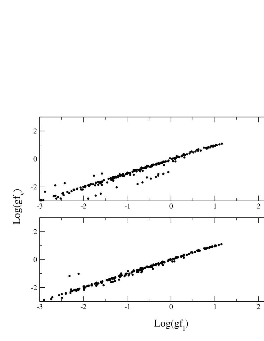
Figure 1: log $gf_{V}$ plotted against log $gf_{L}$ for transitions between energy levels. Panels (a) and (b) show the results computed without polarization interaction and with polarization interaction respectively

In the calculation of radiative rates, fine tuning of eigenstates is performed with term energy corrections (TEC), where the improved relativistic wave function, $\psi_{i}^{R}$, is obtained in terms of the non-relativistic functions

$$\psi_{i}^{R}=\psi_{i}^{LS}+\sum_{j\neq i}\psi_{j}^{LS}\times\frac{\langle\psi_{j}^{LS}\mid H_{bp}\mid\psi_{i}^{LS}\rangle}{E_{i}^{LS}-E_{j}^{LS}},$$ (4)

with the $LS$ energy differences $E_{i}^{LS}-E_{j}^{LS}$ adjusted to fit weighted averaged energies of the experimental multiplets (Zeippen et al. 1977).

In our best target representation, which accounts for the interaction between the valence electron and the core, the theoretical energies for all the 23 terms are typically within 2% of the experimental values before any further empirical correction. After TEC, the agreement with experimental energies is better than 1%.

For dipole-allowed transitions, spontaneous decay rates are given by

$$A_{ij}^{E1}=2.6774\times 10^{9}(E_{i}-E_{j})^{3}\frac{1}{g_{i}}S^{E1}_{ij}\ \ (s^{-1}),$$ (5)

while for forbidden transitions we consider electric quadrupole (E2) and magnetic dipole (M1) transition rates given by

$$A_{ij}^{E2}=2.6733\times 10^{3}(E_{i}-E_{j})^{5}\frac{1}{g_{i}}S^{E2}_{ij}\ \ (s^{-1})$$ (6)

and

$$A_{ij}^{M1}=3.5644\times 10^{4}(E_{i}-E_{j})^{3}\frac{1}{g_{i}}S^{M1}_{ij}\ \ (s^{-1}).$$ (7)

Here, $g_{i}$ is the statistical weight of the upper initial level $i$, $S_{ij}$ is the line strength and $E$ is the energy in Rydbergs.

Eqns.(5,6 and 7) show that the transition rates are sensitive to the accuracy of the energy levels, particularly for forbidden transitions among nearby levels. Thus, we perform further adjustments to the transitions rates by correcting our best calculated energies to experimental values.

In Fig. 1 we plot the $gf$-values for dipole allowed transitions among fine structure levels computed in the length gauge vs. those in the velocity gauge. We present the $gf$-values without PI (a) and with PI (b). The overall agreement between the two gauges is around 5% for $\log(gf)$-values greater than $-3$ when accounting for PI and greater than 15% without PI. This is a good indicator of the quality of the dipole allowed radiative data.

In Table 3 we present an extensive comparison between the present results and previous lifetimes for the metastable levels ${\rm 3d\leavevmode\nobreak\ ^{2}D_{5/2}}$ and ${\rm 3d\leavevmode\nobreak\ ^{2}D_{3/2}}$. These levels are of particular astrophysical interest because they yield the prominent spectral lines $\lambda\lambda$ 7293, 7326 Å. Our results including PI and TEC are in excellent agreement with experimental values, while the results that neglect PI are $\sim$10% too low.

Table 3: Lifetimes of the metastable ${\rm 3d\leavevmode\nobreak\ ^{2}D}$ levels of Ca ii

Level	Present		Other	Experiment($\tau$(s))
	w/o PI	PI
${\rm 3d\leavevmode\nobreak\ ^{2}D_{3/2}}$	0.926	1.107	1.0811	1.176$\pm$0.0115
			1.162
			1.273
			0.984
			1.1965
${\rm 3d\leavevmode\nobreak\ ^{2}D_{5/2}}$	0.901	1.08	1.0581	1.168$\pm$0.0095
			1.142	1.152$\pm$0.0207
			1.243	1.100$\pm$0.0188
			0.954	1.054$\pm$0.0619
			1.1655	1.149$\pm$0.01410
			1.0456	1.064$\pm$0.01711
			1.1411

¹Zeippen (1990), ²Vaeck et al. (1992), ³Guet & Johnson (1991), ⁴Ali & Kim (1988), ⁵Kreuter et al. (2005), ⁶Liaw (1995), ⁷Knoop et al. (2004), ⁸Block et al. (1999), ⁹Arbes et al. (1994), ¹⁰Staanum et al. (2004), ¹¹Gudjons et al. (1996)

In Table 4 we compare the calculated lifetimes for short-lived levels of Ca ii from the present calculations with other theoretical and experimental values. For the lower levels ($4p\leavevmode\nobreak\ ^{2}P^{\rm o}_{1/2}$ and $4p\leavevmode\nobreak\ ^{2}P^{\rm o}_{3/2}$) the effect of polarization interaction is $\sim$20%. Overall, the differences between the results of our best model and experimental values are less than 5%, except for the level $5d\leavevmode\nobreak\ ^{2}D_{5/2}$. For this level, our result agrees with previous independent calculations but is about 40% below the experimental values of Andersen et al. (1970). A new measurement of this lifetime would be very important.

Table 4: Ca ii lifetimes (in ns). The second column gives the results with neither PI (w/o PI) nor TECs (w/o TECs), the third column gives the results without PI (w/o PI) but with TEC, the fourth columns gives results with PI but no TEC, and the fifth column shows the results with both PI and TEC. Theoretical (Other) and experimental (Experiment) values from other authors are given in the sixth and seventh columns, respectively.

Level	Present				Other	Experiment
	w/o PI		PI
	w/o TEC	TEC	w/o TEC	TEC
${\rm 4p\leavevmode\nobreak\ ^{2}P^{o}_{1/2}}$	6.978	5.734	6.697	6.837	6.44a	7.07$\pm 0.07^{b}$
					6.87b	7.5$\pm$0.5g
					6.39c	6.62$\pm$0.35h
					6.94d	6.95$\pm$0.18i
					7.045e	7.098$\pm$0.020m
					7.047l
${\rm 4p\leavevmode\nobreak\ ^{2}P^{o}_{3/2}}$	6.797	5.577	6.508	6.649	6.28a	6.87$\pm$0.06b
					6.24b	7.4$\pm$0.6g
					6.21c	6.68$\pm$0.35h
					6.75d	6.72$\pm$0.20j
					6.852e	6.61$\pm$0.30k
					6.833l	6.87$\pm$0.18i
						6.924$\pm$0.019m
${\rm 4d\leavevmode\nobreak\ ^{2}D_{3/2}}$	2.963	2.779	2.781	2.934	2.868e
${\rm 4d\leavevmode\nobreak\ ^{2}D_{5/2}}$	2.981	2.799	2.800	2.952	2.886e
${\rm 4f\leavevmode\nobreak\ ^{2}F^{o}_{5/2}}$	3.625	2.656	3.487	3.451	3.895e
${\rm 4f\leavevmode\nobreak\ ^{2}F^{o}_{7/2}}$	3.625	2.654	3.486	3.448	3.897e
${\rm 5s\leavevmode\nobreak\ ^{2}S_{1/2}}$	4.310	3.833	3.886	3.982	4.13a	4.3$\pm$0.4g
					4.153e
					3.85f
${\rm 5p\leavevmode\nobreak\ ^{2}P^{o}_{1/2}}$	40.195	34.903	36.541	35.174	33.78a
					36.200e
${\rm 5p\leavevmode\nobreak\ ^{2}P^{o}_{3/2}}$	38.987	33.755	35.783	34.401	33.92a
					35.349e
${\rm 5d\leavevmode\nobreak\ ^{2}D_{3/2}}$	5.960	5.625	5.895	6.102	6.148e
${\rm 5d\leavevmode\nobreak\ ^{2}D_{5/2}}$	6.002	5.669	5.944	6.154	6.199e	4.3$\pm$0.2g
${\rm 6s\leavevmode\nobreak\ ^{2}S_{1/2}}$	7.007	6.390	6.391	6.457	6.90a
					6.766e
					6.51f
${\rm 6p\leavevmode\nobreak\ ^{2}P^{o}_{1/2}}$	114.06	98.569	93.141	90.173	58.95 a
					100.254e
${\rm 6p\leavevmode\nobreak\ ^{2}P^{o}_{3/2}}$	111.23	95.788	92.262	89.129	43.06 a
					99.675e

^aHafner & Schwarz (1978), ^bGosselin et al. (1988a), ^cWiese et al. (1969), ^dGuet & Johnson (1991), ^eTheodosiou (1989), ^fBlack et al. (1972), ^gAndersen et al. (1970), ^hAnsbacher et al. (1985), ⁱGosselin et al. (1988b), ^jSmith & Gallagher (1966), ^kRambow & Schearer (1976), ^lLiaw (1995), ^mJin & Church (1993)

In Table 5 we present a comparison between calculated and experimental oscillator strengths in absorption. For the calculated oscillator strengths we choose the most complete and representative set of values as well as the most cited. We compare with previous calculations by Vaeck et al. (1992) where they use a multiconfiguration Hartree-Fock method with core polarization included variationally (SECP) using a model potential of the form described first by Baylis (1977) and then reviewed by Hibbert (1989). We also compare with Theodosiou (1989) who used a Hartree-Slater (HS) core potential with semiempirical corrections, Guet & Johnson (1991) who used relativistic many-body theory and Brage et al. (1993) using an orthogonal Breit-Pauli MCHF method. We also compare with experimental values of Gallagher (1967) who used the Hanle-effect technique with optical excitation from the ion ground state. The inclusion of PI can affect the oscillator strengths by up to 12%. One finds very good agreement between the present calculation, previous calculations and experimental values.

Table 5: Oscillator strengths for Ca ii. The oscillator strengths from previous calculations of Vaeck et al. (1992), Theodosiou (1989), Guet & Johnson (1991) and Brage et al. (1993), and experimental data from Gallagher (1967) are also given.

Transition	Present		Vaeck	Theodosiou	Guet	Brage	Experiments
	w/o PI	PI
${\rm 4s\leavevmode\nobreak\ S_{1/2}-4p\leavevmode\nobreak\ P^{o}_{1/2}}$	0.364	0.323	0.318	0.316	0.320	0.321
${\rm 4s\leavevmode\nobreak\ ^{2}S_{1/2}-4p\leavevmode\nobreak\ ^{2}P^{o}_{3/2}}$	0.734	0.652	0.641	0.637	0.645	0.649	0.66$\pm$0.02
${\rm 3d\leavevmode\nobreak\ ^{2}D_{3/2}-4p\leavevmode\nobreak\ ^{2}P^{o}_{1/2}}$	0.0478	0.0537	0.0547	0.0473	0.0494	0.0524
${\rm 3d\leavevmode\nobreak\ ^{2}D_{3/2}-4p\leavevmode\nobreak\ ^{2}P^{o}_{3/2}}$	0.0098	0.0110	0.0112	0.0096	0.0101	0.0107	0.0088$\pm$0.001
${\rm 3d\leavevmode\nobreak\ ^{2}D_{5/2}-4p\leavevmode\nobreak\ ^{2}P^{o}_{3/2}}$	0.0584	0.0656	0.0666	0.0574	0.0601	0.0637	0.053$\pm$0.006

In Table 6 we present our electric quadrupole and magnetic dipole transitions probabilities computed including PI and TEC. We compare these with previous calculations of Zeippen (1990), who used a two-step minimization procedure and semi-empirical term energy corrections using the computer program SUPERSTRUCTURE, Ali & Kim (1988) who used the multiconfiguration Dirac-Fock formalism and Vaeck et al. (1992). Our results are in good agreement (within $\sim$2%) with Zeippen (1990) and within $\sim$13% and $\sim$8% with respect to Ali & Kim (1988) and Vaeck et al. (1992).

Table 6: Electric quadrupole (E2) and magnetic dipole (M1) transitions probabilities of [Ca ii]. We compare our results with previous calculated values of Zeippen (1990), Ali & Kim (1988) and Vaeck et al. (1992).

A($s^{-1}$)	Type	Present	Zeippen	Ali and Kim	Vaeck
${\rm 3d\leavevmode\nobreak\ ^{2}D_{3/2}-4s\leavevmode\nobreak\ ^{2}S_{1/2}}$	E2	0.905	0.925	1.02	0.84
${\rm 3d\leavevmode\nobreak\ ^{2}D_{5/2}-4s\leavevmode\nobreak\ ^{2}S_{1/2}}$	E2	0.928	0.945	1.05	0.86
${\rm 3d\leavevmode\nobreak\ ^{2}D_{5/2}-3d\leavevmode\nobreak\ ^{2}D_{3/2}}$	M1	2.41$\times 10^{-6}$	2.45$\times 10^{-6}$	2.45$\times 10^{-6}$

2.3 Scattering calculations

In the close coupling (CC) approximation the total wave function of the electron-ion system is represented as

$$\psi(E;LS\pi)=A\sum_{i}\chi_{i}\theta_{i}+\sum_{j}c_{j}\Phi_{j}$$ (8)

where $\chi_{i}$ is the target ion wave function in a specific state $LS_{i}$, $\theta_{i}$ is the wave function of the free electron, $\Phi_{j}$ are short range correlation functions for the bound (e+ion) system, and $A$ is the antisymetrization operator.

The variational procedure gives rise to a set of coupled integro-differential equations that are solved with the R-matrix technique (Burke et al. 1971; Berrington et al. 1978, 1995) within a box of radius $r\leq a$. In the asymptotic region, $r>a$, exchange between the outer electron and the target ion can be neglected and if all long-range potentials beyond Coulombic are also neglected, the reactance $K$-matrix and the scattering $S$-matrix are obtained by matching at the boundary the inner-radial functions to linear combinations of the outer-region Coulomb solutions. Later, the contributions of long-range potentials to the collision strengths are included perturbatively (Griffin et al. 1998).

We use the $LS$-coupling R-matrix method that includes mass-velocity and Darwin operators and the polarization model potential. Note that the scattering calculations include one-body relativistic operators while the atomic structure calculations using AUTOSTRUCTURE include two-body operators of the Breit-Pauli Hamiltonian namely (two-body) fine-structure operators and (two-body) non-fine-structure operators.

The $S$-matrix elements determine the collision strength for a transition from an initial target state $i$ to a final target state $f$,

$$\Omega_{if}=\frac{1}{2}\sum w|S_{if}-\delta_{if}|,$$ (9)

where $w=(2L+1)(2S+1)$ or $(2J+1)$ depending on the coupling scheme, and the summation runs over the partial waves and channels coupling the initial and final states of interest.

In order to derive fine-structure results out of the $LS$-coupling calculation we employ the intermediate-coupling frame transformation (ICFT) method of Griffin et al. (1998). The ICFT method uses the multi-channel quantum defect theory (MQDT) to generate the LS-coupled unphysical $K$-matrices. In this approach one treats all scattering channels as open and calculates the term-coupling coefficients (TCCs) to transform the unphysical $K$-matrices to full intermediate coupling. Finally, we can generate the physical $K$-matrices on a fine energy mesh. Because all channels are treated as open this method eliminates the problems associated with the transformation of the physical $S$-matrices with closed channels and consequently yields accurate results for both background and resonances of the collision strengths at all energies.

The computations were carried out with the RMATRX package of codes (Berrington et al. 1995) and also include the dipole polarization potential for the interaction of the valence electron and the core. The set of (N+1)-electron wave functions to the right of the CC expansion in Eq. (8) includes all the configurations that result from adding an additional electron to the target configurations.

In Fig. 2 we compare the collision strengths for different target expansions. For the various close-coupling expansions we include all the terms that arise from the $n$=3, 4, 5, 6, 7 and 8 configurations. It is interesting to note that by increasing the number of terms in the close-coupling expansion the resonances tend to become better organized and blended, leading to regular broad series of structures. This is because of the increasing number of channels for decay of autoionizing levels. We adopt the expansion up to n=8 for all further calculations.

Figure 2: Comparison between collision strengths for the Ca ii ion with different CC expansions for the ${\rm 3d\leavevmode\nobreak\ ^{2}D_{3/2}-4s\leavevmode\nobreak\ ^{2}S_{1/2}}$ (upper panel) and ${\rm 4p\leavevmode\nobreak\ ^{2}P^{o}_{1/2}-4s\leavevmode\nobreak\ ^{2}S_{1/2}}$ (lower panel) transitions. $n$ represents the principal quantum number for the valence electron.

Partial wave contributions to the summation in Eqn. 3 were included from 162 $SL\pi$ total symmetries with angular momentum $L=0-40$, total multiplicities $(2S+1)=1$ and 3, and parities even and odd. As for the number of continuum orbitals per angular momentum we found necessary to include up to $40$. The collision strengths were “topped up” with estimates of the contributions of higher partial waves for the optically allowed transitions based on the Coulomb-Bethe approximation Burgess (1974) and for non-allowed transitions we approximate the top-up with a geometric series. It was verified that by explicitly including partial waves up to $L=40$ such “top ups” amount to less than 10% of the total collision strengths for all transitions with the exception of the transitions $n$g-$n$f (for $n>$6) for which the top up is greater than $20\%$. This is because of the very small energy difference between these terms.

In order to check for convergence of the partial wave expansion one needs to study the high energy behavior for the collision strengths ($\Omega$). In Fig. 3 we plot reduced collision strengths ($\Omega_{r}$) as function of reduced energy ($E_{r}$) following the procedure describe by Burgess & Tully (1992). This approach allows us to visualize the complete range of energies mapped onto the interval [0,1]. The last point in these graphs represents the infinite energy limit of the collision strengths ($E\rightarrow\infty$). For this plot we adopt a scaling parameter $C=1.5$. These plots show good progression of the collision strengths toward the high energy limit, which gives confidence on the consistency and quality of the data.

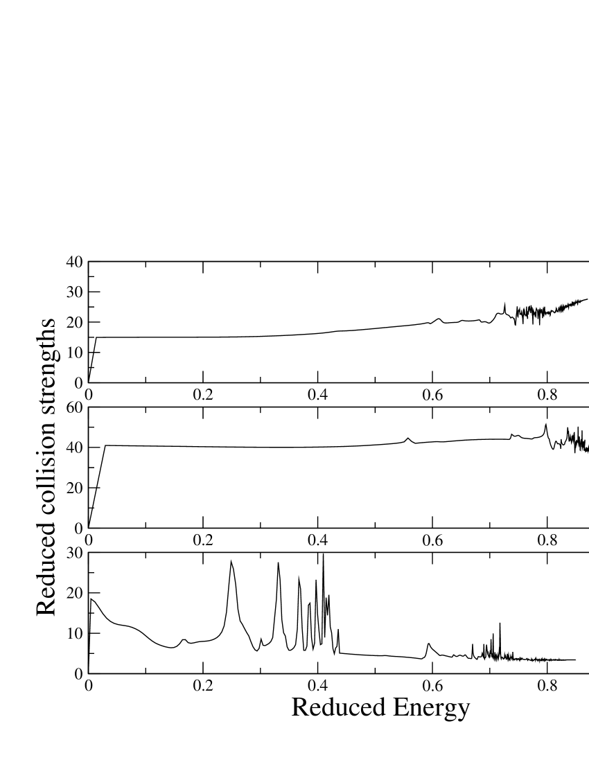
Figure 3: Reduced collision strengths for the ${\rm 4s\leavevmode\nobreak\ ^{2}S\leavevmode\nobreak\ -\leavevmode\nobreak\ 4p\leavevmode\nobreak\ ^{2}P^{o}}$ (upper panel), ${\rm 3d\leavevmode\nobreak\ ^{2}D\leavevmode\nobreak\ -\leavevmode\nobreak\ 4p\leavevmode\nobreak\ ^{2}P^{o}}$ (middle panel) and ${\rm 4s\leavevmode\nobreak\ ^{2}S\leavevmode\nobreak\ -\leavevmode\nobreak\ 3d\leavevmode\nobreak\ ^{2}D}$ (lower panel) transitions.

Fig. 4 shows the collision strength computed with and without polarization interaction for a sample of transitions between levels of the lowest four multiplets. One can see that the core polarization has an important effect on the collision strengths. We verified through various calculations that such effects come almost entirely from the change in the radial wave functions of the target, while the effects of the dipole polarization operator in the scattering matrix is nearly negligible. The same conclusion was derived by Mitroy et al. (1988).

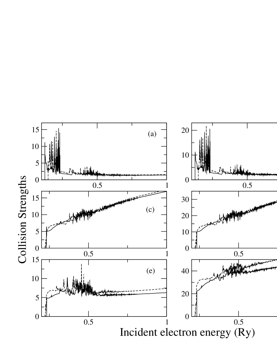
Figure 4: Comparison between collision strengths for the Ca ii ion. The solid and dashed lines depict the results with and without model potential interaction respectively. The transitions are: (a) ${\rm 3d\leavevmode\nobreak\ ^{2}D_{3/2}-4s\leavevmode\nobreak\ ^{2}S_{1/2}}$; (b) ${\rm 3d\leavevmode\nobreak\ ^{2}D_{5/2}-4s\leavevmode\nobreak\ ^{2}S_{1/2}}$; (c) ${\rm 4p\leavevmode\nobreak\ ^{2}P^{o}_{1/2}-4s\leavevmode\nobreak\ ^{2}S_{1/2}}$; (d) ${\rm 4p\leavevmode\nobreak\ ^{2}P^{o}_{3/2}-4s\leavevmode\nobreak\ ^{2}S_{1/2}}$; (e) ${\rm 3d\leavevmode\nobreak\ ^{2}D_{3/2}-4p\leavevmode\nobreak\ ^{2}P^{o}_{3/2}}$ and (f) ${\rm 3d\leavevmode\nobreak\ ^{2}D_{5/2}-4p\leavevmode\nobreak\ ^{2}P^{o}_{3/2}}$.

The collision strengths were calculated at $22000$ energy points from 0 to 4 Ry, with a resolution of $10^{-5}$ Ry in the region with resonances and $5\times 10^{-3}$ Ry at higher energies. This number of points was found sufficient to resolve most resonance structures for accurate calculations of effective collision strengths for temperatures above $\sim$5000 K.

A dimensionless thermally-averaged effective collision strength results from integrating the collision strength over a Maxwellian distribution of electron velocities

$$\Upsilon_{if}=\int_{0}^{\infty}\Omega_{if}\exp{(-\epsilon_{f}/kT)}$d$(\epsilon_{f}/kT),$$ (10)

where $\epsilon_{f}$ is the kinetic energy of the outgoing electron, $T$ the electron temperature in Kelvin and $k=6.339\times 10^{-6}$ Ry/K is the Boltzmann constant.

In Table 7 we compare the present effective collision strengths for the 4s$\to$ 4p transition of Ca ii. We show the values obtained by Osterbrock & Wallace (1977) where they used experimental results of Taylor & Dunn (1973), as reduced to collision strengths by Seaton (1975). We also present the values from Burgess et al. (1995) as we use their five point cubic spline fitting parameters to tabulate the $\Upsilon(T)$ using the procedure described in Burgess & Tully (1992). We compare them with our present calculation without PI in the target representation and in the scattering calculations (w/o PI); without PI in the R-matrix calculations only (PI-S) and with PI. Our best results agree within 11% of Osterbrock & Wallace (1977) values. On the other hand, the results of Burgess et al. (1995) obtained with the non-exchange distorted wave approximation appear overestimated by $\sim$50%. In this calculation, the Ca II target is represented in the frozen core approximation neglecting polarization. As we pointed out before the main contribution of the dipole polarization potential is in the representation of the target ion. Further, our effective collision strengths when neglecting polarization are overestimated by $30\%$, in closer agreement with Burgess et al. (1995).

Table 7: Effective collision strengths for the 4s ²S  - 4p ²P^o transition Ca ii. The first three lines correspond to results of the present calculations for the cases of no PI in either the target orbitals of scattering calculation (w/o PI), PI in the scattering calculation only (PI-S), and PI in the target and scattering calculations (PI). These results are compared with values deduced from experimental cross sections (Osterbrock & Wallace 1977) (OW) and the most recent theoretical calculations (Burgess et al. 1995) (BCT).

$T\leavevmode\nobreak\ (k)$
5000	10000	15000	20000
19.03	20.82	22.45	24.03	w/o PI
16.96	19.34	21.35	23.13	PI-S
17.07	19.44	21.45	23.23	PI
15.6	17.5	19.2	20.8	OW
24.87	27.50	29.88	32.04	BCT

3 Conclusions

We have computed radiative data, collision strengths and effective collision strengths for transitions among 41 levels from the n=3, 4, 5, 6, 7 and 8 configurations of Ca ii. The radiative data were calculated using the Thomas-Fermi-Dirac central potential with a model core potential that account for dipole polarization interaction of the valence electron with the core. We also present an extensive comparison between our results and the most recent experiments and calculations for the lifetimes of Ca ii.

Effective collision strengths are available for various temperatures that expand from 3000 K to 38000 K. The whole set of data reported here including energy levels, infinite energy limit Born collision strengths, transition probabilities and effective collision strengths can be obtained in electronic form at the CDS via anonymous ftp to cdsarc.u-strasbg.fr (130.79.128.5), via http://cdsweb.u-strasbg.fr/cgi-bin/qcat?J/A+A/ or by request to the authors.

References

- Ali & Kim (1988) Ali, M. A. & Kim, Y.-K. 1988, Phys. Rev. A, 38, 3992
- Andersen et al. (1970) Andersen, T., Desesquelles, J., Jessen, K. A., & Sorensen, G. 1970, J. Quant. Spectrosc. Radiat. Transfer., 10, 1143
- Ansbacher et al. (1985) Ansbacher, W., Inamdar, A. S., & Pinnington, E. H. 1985, Physics Letters A, 110, 383
- Arbes et al. (1994) Arbes, F., Benzing, M., Gudjons, T., Kurth, F., & Werth, G. 1994, Zeitschrift fur Physik D Atoms Molecules Clusters, 29, 159
- Badnell (1986) Badnell, N. R. 1986, J. Phys. B: At. Mol. Opt. Phys, 19, 3827
- Badnell (1997) Badnell, N. R. 1997, J. Phys. B: At. Mol. Opt. Phys, 30, 1
- Bautista (2001) Bautista, M. A. 2001, A&A, 365, 268
- Bautista (2004) Bautista, M. A. 2004, A&A, 420, 763
- Bautista & Pradhan (1998) Bautista, M. A. & Pradhan, A. K. 1998, in Revista Mexicana de Astronomia y Astrofisica Conference Series, ed. R. J. Dufour & S. Torres-Peimbert, 163
- Baylis (1977) Baylis, W. E. 1977, J. Phys. B: At. Mol. Opt. Phys, 10, L583
- Berrington et al. (1978) Berrington, K. A., Burke, P. G., Le Dourneuf, M., et al. 1978, Computer Physics Communications, 14, 367
- Berrington et al. (1995) Berrington, K. A., Eissner, W. B., & Norrington, P. H. 1995, Computer Physics Communications, 92, 290
- Black et al. (1972) Black, J. H., Weisheit, J. C., & Laviana, E. 1972, ApJ, 177, 567
- Block et al. (1999) Block, M., Rehm, O., Seibert, P., & Werth, G. 1999, European Physical Journal D, 7, 461
- Brage et al. (1993) Brage, T., Froese Fischer, C., Vaeck, N., Godefroid, M., & Hibbert, A. 1993, Phys. Scr, 48, 533
- Burgess (1974) Burgess, A. 1974, J. Phys. B: At. Mol. Opt. Phys, 7, L364
- Burgess et al. (1995) Burgess, A., Chidichimo, M. C., & Tully, J. A. 1995, A&A, 300, 627
- Burgess & Tully (1992) Burgess, A. & Tully, J. A. 1992, A&A, 254, 436
- Burke et al. (1971) Burke, P. G., Hibbert, A., & Robb, W. D. 1971, J. Phys. B: At. Mol. Opt. Phys, 4, 153
- Chidichimo (1981) Chidichimo, M. C. 1981, J. Phys. B: At. Mol. Opt. Phys, 14, 4149
- Eissner et al. (1974) Eissner, W., Jones, M., & Nussbaumer, H. 1974, Computer Physics Communications, 8, 270
- Eissner & Nussbaumer (1969) Eissner, W. & Nussbaumer, H. 1969, J. Phys. B: At. Mol. Opt. Phys, 2, 1028
- Ferland & Persson (1989) Ferland, G. J. & Persson, S. E. 1989, ApJ, 347, 656
- Gallagher (1967) Gallagher, A. 1967, Physical Review, 157, 24
- Gosselin et al. (1988a) Gosselin, R. N., Pinnington, E. H., & Ansbacher, W. 1988a, Phys. Rev. A, 38, 4887
- Gosselin et al. (1988b) Gosselin, R. N., Pinnington, E. H., & Ansbacher, W. 1988b, Nuclear. Instrum. Methods, 31, 305
- Griffin et al. (1998) Griffin, D. C., Badnell, N. R., & Pindzola, M. S. 1998, J. Phys. B: At. Mol. Opt. Phys, 31, 3713
- Gudjons et al. (1996) Gudjons, T., Hilbert, B., Seibert, P., & Werth, G. 1996, Europhysics Letters, 33, 595
- Guet & Johnson (1991) Guet, C. & Johnson, W. R. 1991, Phys. Rev. A, 44, 1531
- Hafner & Schwarz (1978) Hafner, P. & Schwarz, W. H. E. 1978, J. Phys. B: At. Mol. Opt. Phys, 11, 2975
- Hibbert (1989) Hibbert, A. 1989, Phys. Scr, 39, 574
- Hummer et al. (1993) Hummer, D. G., Berrington, K. A., Eissner, W., et al. 1993, A&A, 279, 298
- Jin & Church (1993) Jin, J. & Church, D. A. 1993, Physical Review Letters, 70, 3213
- Joly (1989) Joly, M. 1989, A&A, 208, 47
- Jones (1970) Jones, M. 1970, J. Phys. B: At. Mol. Opt. Phys, 3, 1571
- Jones (1971) Jones, M. 1971, J. Phys. B: At. Mol. Opt. Phys, 4, 1422
- Kennedy et al. (1978) Kennedy, J. V., Myerscough, V. P., & McDowell, M. R. C. 1978, J. Phys. B: At. Mol. Opt. Phys, 11, 1303
- Knoop et al. (2004) Knoop, M., Champenois, C., Hagel, G., et al. 2004, European Physical Journal D, 29, 163
- Kreuter et al. (2005) Kreuter, A., Becher, C., Lancaster, G. P., et al. 2005, Phys. Rev. A, 71, 032504
- Liaw (1995) Liaw, S.-S. 1995, Phys. Rev. A, 51, 1723
- Meléndez & Bautista (2005) Meléndez, M. & Bautista, M. A. 2005, A&A, 436, 1123
- Mitroy et al. (1988) Mitroy, J., Griffin, D. C., Norcross, D. W., & Pindzola, M. S. 1988, Phys. Rev. A, 38, 3339
- Norcross & Seaton (1976) Norcross, D. W. & Seaton, M. J. 1976, J. Phys. B: At. Mol. Opt. Phys, 9, 2983
- Osterbrock & Wallace (1977) Osterbrock, D. E. & Wallace, R. K. 1977, Astrophys. Lett., 19, 11
- Rambow & Schearer (1976) Rambow, F. H. K. & Schearer, L. D. 1976, Phys. Rev. A, 14, 1735
- Rauscher & Marcy (2006) Rauscher, E. & Marcy, G. W. 2006, PASP, 118, 617
- Saraph (1970) Saraph, H. E. 1970, J. Phys. B: At. Mol. Opt. Phys, 3, 952
- Seaton (1975) Seaton, M. J. 1975, Advances Atom. Molec. Phys, 11, 83
- Shields et al. (1999) Shields, J. C., Pogge, R. W., & de Robertis, M. M. 1999, in ASP Conf. Ser. 175: Structure and Kinematics of Quasar Broad Line Regions, ed. C. M. Gaskell, W. N. Brandt, M. Dietrich, D. Dultzin-Hacyan, & M. Eracleous, 353
- Smith & Gallagher (1966) Smith, W. W. & Gallagher, A. 1966, Physical Review, 145, 26
- Staanum et al. (2004) Staanum, P., Jensen, I. S., Martinussen, R. G., Voigt, D., & Drewsen, M. 2004, Phys. Rev. A, 69, 032503
- Taylor & Dunn (1973) Taylor, P. O. & Dunn, G. H. 1973, Phys. Rev. A, 8, 2304
- Theodosiou (1989) Theodosiou, C. E. 1989, Phys. Rev. A, 39, 4880
- Vaeck et al. (1992) Vaeck, N., Godefroid, M., & Froese Fischer, C. 1992, Phys. Rev. A, 46, 3704
- Waller (1926) Waller, I. 1926, Z. f. Phys, 38, 635
- Wiese et al. (1969) Wiese, W. L., Smith, M. W., & Miles, B. M. 1969, Atomic transition probabilities. Vol. 2: Sodium through Calcium. A critical data compilation (NSRDS-NBS, Washington, D.C.: US Department of Commerce, National Bureau of Standards, —c 1969)
- Zapesochnyǐ et al. (1975) Zapesochnyǐ, I. P., Kel’Man, V. A., Imre, A. I., Dashchenko, A. I., & Danch, F. F. 1975, Soviet Physics JETP, 42, 989
- Zatsarinny et al. (1991) Zatsarinny, O. I., Lengyel, V. I., & Masalovich, E. A. 1991, Phys. Rev. A, 44, 7343
- Zeippen (1990) Zeippen, C. J. 1990, A&A, 229, 248
- Zeippen et al. (1977) Zeippen, C. J., Seaton, M. J., & Morton, D. C. 1977, MNRAS, 181, 527