Abstract

Proposed by Wolfgang Pauli more than 80 years ago, the exclusion principle has been proven to have a far-reaching consequence, from femtoscopic world to macroscopic, super-dense, and fully relativistic physics. Starting from this principle, we discuss two interesting research topics, which have currently drawn considerable attention in the nuclear- and astrophysics communities; the hypernuclear and neutron star physics. Special attention is given to the electromagnetic production of the hypertriton and the consequences of the neutrino electromagnetic properties in dense matter. We also touch on the new arena which could also be fascinating for physicists; the econophysics.

1 Pauli Exclusion Principle and Its Consequence

1.1 Historical Background

Most of us started to be acquainted with the Pauli exclusion principle at high-school, when we learned about atomic shells in the chemistry or in the physics course. Probably, many of us are ignorant that the discovery of the exclusion principle is in fact intimately related to the conception of the electron spin and the development of quantum mechanics. If we try to comprehend the motivation of Wolfgang Pauli behind this great discovery, for which he was awarded with the Nobel Prize in 1945, then we will find that it was to answer the problem of explaining the observed atomic spectra and the “anomalous Zeeman effect” [1]. At that time these transitions were particularly confusing, because some of them (e.g., the Sodium atom) exhibit doublet transitions, whereas some others (e.g., the Magnesium atom) show either singlet or triplet transitions [2]. Furthermore, the anomalous Zeeman effect yields a doublet splitting, contrary to the what was hitherto known by the spectroscopists as triplet splitting. Another disturbing fact to Pauli was the question as to why all electrons for an atom in its ground state were not bound in the innermost shell, a problem which had been emphasized even by Niels Bohr as his fundamental problem.

Before 1924, Arnold Sommerfeld, Alfred Landé, and Pauli himself realized that the answer to these problems was the existence of a new (the fourth, after $n,\ell$ and $m$, to be more precise) quantum number. Sommerfeld and Landé considered this number as an intrinsic property of the atomic core, without specifying whether it is the nucleus or the nucleus plus inner electrons. This point of view was then considered by Pauli as rather orthodox.

In 1924 Pauli published an objection to this argument [4]. Instead of considering the properties of the atomic core, Pauli proposed a new quantum property of the electron, which he called “two-valuedness not describable classically.” Using this idea Pauli was able to reduce the complicated numbers of electrons in closed subgroups to the simple one, once this fourth quantum property is introduced. Nevertheless, with the exception of few famous spectroscopists, nobody could easily follow this idea, since there was no analogy in terms of mechanical model. This difficulty was then remedied by the concept of electron spin proposed by George E. Uhlenbeck and Samuel A. Goudsmit, who tried to explain the experimental result of Otto Stern and Walther Gerlach [5]. It was said that after some discussions with Lorentz, they tried to withdraw their paper, but it was too late and the paper was published! With this concept, i.e. by assuming that the spin quantum number of electron as $\frac{1}{2}$, it is then possible to understand the doublet splitting in the anomalous Zeeman effect [6]. Since then the idea of exclusion principle was always closely connected with the spin.

Figure 1: Wolfgang Pauli (1900-1958), the 1945 Nobel laureate for “the discovery of the exclusion principle”[3].

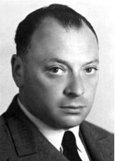
Pauli formulated his exclusion principle comprehensively in 1925 [7]. At about the same time, several milestones in quantum mechanics were achieved. The most important and relevant one to the present discussion is the formulation of the quantum mechanics by Werner Heisenberg [8]. According to Heisenberg, quantum mechanics leads to qualitatively different conclusions for distinguishable particles than for indistinguishable particles. It was found that for indistinguishable particles the wave function must be either symmetric or antisymmetric. Pauli considered the antisymmetric one as the appropriate wave mechanical formulation of the exclusion principle, since an antisymmetric wave function containing two particles in the same state is equal to zero.

The first indication that proton has spin $\frac{1}{2}$ was obtained from the investigation of the anomaly in the specific heat of the molecular hydrogen in 1927 [9]. Later on, this was confirmed by Stern by using a Stern-Gerlach type experiment. In 1932, the neutron was discovered by Frederic and Irène Joliot-Curie along with James Chadwick. Two years later, by dissociating deuteron with gamma ray, $\gamma+d\to n+p$, Chadwick and Maurice Goldhaber were able to show that a deuteron was made of a proton and a neutron. From its spectrum it was known that the deuteron has spin 1. Hence, we know that the neutron has also spin $\frac{1}{2}$ and both proton and neutron obey the Pauli exclusion principle.

Although for us the exclusion principle is quite clear and understandable, Pauli himself was disappointed with his finding, since he said that he was unable to give a logical reason or to deduce the principle from a more general assumption. He was hoping that the development of quantum mechanics will also rigorously deduce the principle, but he eventually found that it was not the case [1].

1.2 The Degeneracy Force

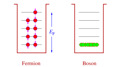
Let us begin with a simple gedanken experiment, i.e., we drop a number of fermions into a square well potential. We repeat the same experiment for a number of bosons. As we expected, the result is shown in Fig. 2. However, to understand why the fermions sitting above the ground state do not collapse to the lowest state as in the case of bosons, we need to understand the degeneracy force, a kind of force which maintains such formation.

Figure 2: If nine fermions and nine bosons are “dropped” into square well potentials, they will organize themselves in quite different ways. This happens because the fermions always obey the Pauli exclusion principle.

Consider two particles $a$ and $b$ located at $x_{1}$ and $x_{2}$. The wave function of such a system can be written as [10]

$$\Psi(x_{1},x_{2}) = \psi_{a}(x_{1})\,\psi_{b}(x_{2})~{},$$ (1)

where both $\psi_{a}$ and $\psi_{b}$ are normalized to unity. Let us now calculate the expectation value of the “distance” between the two particles, i.e.,

$$\langle(x_{1}-x_{2})^{2}\rangle~{}=~{}\langle x_{1}^{2}\rangle+\langle x_{2}^{2}\rangle-2\langle x_{1}x_{2}\rangle~{}.$$ (2)

Using the wave function given in Eq. (1) we can calculate the first term on the r.h.s. of Eq. (2),

$$\langle x_{1}^{2}\rangle~{}=~{}\int dx_{1}\,x_{1}^{2}\,|\psi_{a}(x_{1})|^{2}\,\underbrace{\int dx_{2}\,|\psi_{b}(x_{2})|^{2}}_{=1}~{}=~{}\int dx~{}x^{2}\,|\psi_{a}(x)|^{2}\,~{}\equiv~{}\langle x^{2}\rangle_{a}~{},$$ (3)

where the subscript $a$ indicates that the expectation value is calculated using the wave function $\psi_{a}(x)$. By following the same procedure we can easily prove that $\langle x_{2}^{2}\rangle=\langle x^{2}\rangle_{b}$ and $\langle x_{1}x_{2}\rangle=\langle x\rangle_{a}\langle x\rangle_{b}$. Therefore, the “distance “ between two distinguishable particles is found to be

$$\langle(x_{1}-x_{2})^{2}\rangle_{\rm dis}~{}=~{}\langle x^{2}\rangle_{a}+\langle x^{2}\rangle_{b}-2\langle x\rangle_{a}\langle x\rangle_{b}~{}.$$ (4)

On the other hand, the wave function for two indistinguishable boson or fermion is given by

$$\Psi_{\pm}(x_{1},x_{2})~{}=~{}\frac{1}{\sqrt{2}}\left[\psi_{a}(x_{1})\,\psi_{b}(x_{2})\pm\psi_{a}(x_{2})\,\psi_{b}(x_{1})\right]~{},$$ (5)

where the $+$ and $-$ signs indicate the symmetric (boson) and anti-symmetric (fermion) systems. Using Eq. (5) we can recalculate Eq. (4) and obtain

$$\langle(x_{1}-x_{2})^{2}\rangle_{\pm}~{}=~{}\langle x^{2}\rangle_{a}+\langle x^{2}\rangle_{b}-2\langle x\rangle_{a}\langle x\rangle_{b}\,\mp\,2\,|\langle x\rangle_{ab}|^{2}~{},$$ (6)

where the last term, $\langle x\rangle_{ab}=\int dx\,\psi_{a}^{*}(x)\,x\,\psi_{b}(x)$, clearly depends upon the overlap between the wave functions $\psi_{a}(x)$ and $\psi_{b}(x)$.

By comparing Eqs. (4) and (6) we can conclude that

$$\langle(x_{1}-x_{2})^{2}\rangle_{\pm}~{}=~{}\langle(x_{1}-x_{2})^{2}\rangle_{\rm dis}\,\mp\,2\,|\langle x\rangle_{ab}|^{2}~{}.$$ (7)

This equation is extremely important. Although derived in a quite simple fashion, it shows that two fermions tend to be farther apart than two bosons. This is known as the exchange force (or degeneracy force), which produces a “force of attraction” between identical bosons and a “force of repulsion” between identical fermions. Note that this is not really the force we are familiar with, since there is no mediator which pull or push the particles, instead it is solely a consequence of the (anti)symmetrization required by quantum mechanics.

After we know that identical fermions exhibit “repulsive force”, our next question is certainly “how repulsive is this force?” To answer this question we use the electron gas model, since in this model electrons do not interact via Coulomb force. Furthermore, the electron gas model is a simple model often used in many standard quantum mechanics books [24]. In this model, for $N$ number of electrons, each with a mass of $m$, occupying a volume $V$, the corresponding total energy can be written as

$$E_{\rm tot.}~{}=~{}\frac{\hbar^{2}\pi^{3}}{10mV^{2/3}}\left(\frac{3N}{\pi}\right)^{5/3}~{}.$$ (8)

Using the density $\rho=N/V$ we can calculate the “pressure” produced by the degeneracy force of $N$ electrons and find that

$$p_{\rm deg.}~{}=~{}-\frac{\partial E_{\rm tot.}}{\partial V}~{}=~{}\frac{\hbar^{2}\pi^{3}}{15m}\left(\frac{3\rho}{\pi}\right)^{5/3}~{}.$$ (9)

To get a better feeling on this pressure, let us consider two “chargeless” electrons separated with a distance of 1 Å. The particle density in this case is $\rho\approx 10^{30}$ m^-3. Substituting this value into Eq. (9) we obtain the degeneracy pressure is $p_{\rm deg.}\approx 10^{14}$ N/m². One may suspect that such a huge pressure would be meaningless in an atomic scale, where the typical “area” is of the order of $10^{-20}$ m² and therefore the corresponding force is of the order of $10^{-6}$ N. Nevertheless, one should not forget that at this scale the Coulomb force between two electrons is also of the order of $10^{-8}$ N. The problem, however, turns out to be dramatically interesting on the macroscopic scale where we do business with an area greater than 1 km² or $10^{6}$ m². We will encounter this interesting problem when we discuss the neutron star, but first we will introduce the physics of hypernucleus.

Figure 3: A $\Lambda$-hyperon can freely move in the nuclear energy states, without being blocked by the Pauli principle.

2 Introducing a $\Lambda$ Hyperon in the Nucleus; Hypernuclear Physics

2.1 Pauli Principle in the Nucleus

Let us now imagine that we can implant a $\Lambda$ hyperon inside a normal nucleus. Since the $\Lambda$ hyperon is distinguishable from the nucleons (the protons and neutrons which build up the nucleus), it will certainly be free from Pauli blocking (see Fig. 3). Such a nucleus is called a hypernucleus. Hypernucleus is interesting because many new information about the nuclear structure can be obtained by studying the way the $\Lambda$ hyperon localizes inside the nucleus. Another interesting aspect comes from the fact that a free $\Lambda$ hyperon is unstable, it decays in about $10^{-10}$ s primarily to

$$\Lambda~{}\to~{}\left\{\begin{array}[l]{lr}p~{}+~{}\pi^{-}&({\rm branching~{}fraction~{}:}~{}63.9\%)\\ n~{}+~{}\pi^{0}&({\rm branching~{}fraction~{}:}~{}35.8\%)\end{array}\right.~{},$$ (12)

via weak interaction. However, if the $\Lambda$ is embedded in a nucleus, since the low energy nucleon states in the nucleus are already filled, Pauli principle will prevent it from decaying in the usual way as in Eq. (12). Therefore, there must be another mechanism which eventually allows the hypernucleus to decay via a weak process.

The first hypernucleus was observed by Marian Danysz and Jerzy Pniewski, two Polish physicists, in 1953. They used photographic emulsions exposed to the cosmic radiation. These emulsions recorded a break-up event illustrated in Fig. 4. We can understand this event as follows. A highly energetic proton coming from cosmic rays hits a heavy nucleus in the emulsion, causing it to break up into a number of fragments. One of them (marked with f) decays into three charged particles at point B. This decay cannot be interpreted as a normal decay of a highly excited nucleus, since from the track shown in the figure the three particles should have lived for about $10^{-12}$ s, whereas the normal decay of an excited nucleus would take place in about $10^{-22}$ s. Presumably, the event can be interpreted as the decay of the ${}^{8}_{\Lambda}$Be hypernucleus into three charged particles [11],

$${}^{8}_{\Lambda}{\rm Be}~{}\to~{}^{3}{\rm He}~{}+~{}^{4}{\rm He}~{}+~{}n~{}+~{}\pi^{-}~{}.$$ (13)

Figure 4: The first observed hypernucleus. A highly energetic proton $p$ strikes a nucleus at point A in an emulsion, which immediately breaks up into a number of nuclear fragments. All fragments are eventually stopped in the emulsion except the one marked with f. This fragment decays at point B into three charged particles and a neutron. The neutron is not seen in this figure, since it is chargeless. Original figure was taken from Ref. [12].

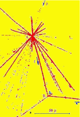
The first hypernucleus was studied in a photographic emulsion exposed to cosmic rays. Nowadays, hypernuclei can be produced in laboratories by using, e.g., hadronic reactions

$$K^{-}~{}+~{}^{A}Z~{}\to~{}^{A}_{\Lambda}{Z}~{}+~{}\pi^{-}~{}~{}~{},~{}~{}~{}~{}~{}\pi^{+}~{}+~{}^{A}Z~{}\to~{}^{A}_{\Lambda}{Z}~{}+~{}K^{+}~{},$$ (14)

or through electromagnetic interactions

$$\gamma~{}+~{}^{A}Z~{}\to~{}^{A}_{\Lambda}{Z}~{}+~{}K^{+}~{}~{}~{},~{}~{}~{}~{}~{}e~{}+~{}^{A}Z~{}\to~{}e^{\prime}~{}+~{}^{A}_{\Lambda}{Z}~{}+~{}K^{+}~{}.$$ (15)

The advantage of using the first reactions, Eq. (14), is that the cross section is large and therefore the corresponding experiments are relatively easy to perform. However, the electromagnetic reactions, Eq. (15), are also invaluable for the study of $\Lambda$ hypernuclei. Since a large momentum is transferred to the recoiled hypernucleus, it will then populate high spin states and, therefore, is very suitable for investigating deeply bound states of a $\Lambda$ hyperon. Furthermore, both spin-flip and non-spin-flip amplitudes are excited with significant cross sections, in contrast to the hadronic reactions. In addition, since a proton is converted to a $\Lambda$ hyperon, hypernuclei that are not accessible by hadronic reactions can be produced. Finally, a comparison between hadronic and electromagnetic reactions allows us to study charge symmetry in the $\Lambda$ hypernuclei [13].

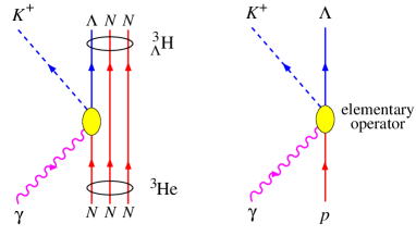
The simplest example is photoproduction of a hypertriton, the lightest hypernucleus. A hypertriton consists of two nucleons and one $\Lambda$ hyperon. Thus, it can be produced by bombarding a ³He target with (real or virtual) photon, as shown in Fig. 5. From this figure it is clear that one of the proton inside the nucleus is converted into a $\Lambda$ hyperon along with a kaon through an elementary process. Therefore, to theoretically calculate the hypertriton photoproduction one needs information about the elementary reaction.

2.2 Elementary Reaction

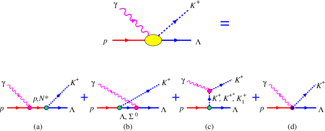
The elementary operator can be modeled in terms of Feynman diagrams at tree-level as shown in Fig. 6. Although higher-order corrections are neglected, most of the hadronic and electromagnetic couplings in these diagrams are in fact not well known. Fortunately, experimental data for the elementary process $\gamma+p\to K^{+}+\Lambda$ have been available since more than 40 years ago. Thus, all unknown coupling constants can be extracted by fitting the calculated observables to these data.

Figure 5: (Left) Photoproduction of a hypertriton. (Right) Photoproduction of a $\Lambda$ hyperon which is called elementary reaction. The amplitude obtained from Feynman diagrams for this reaction is called elementary operator.

Very recently a large number of data have been published by the SAPHIR [14] and CLAS [15] collaborations. These data cover the energy range from reaction threshold up to $W=2.5$ GeV, angular distributions from forward to backward kaon angles, and are significantly more accurate than the previous ones [16]. A comparison between theoretical calculations with small part of these data is shown in Fig. 7. To calculate the differential cross section we have used

$$\frac{d\sigma}{d\Omega} = \frac{|\vec{q}|}{|{\vec{k}}|}~{}\frac{m_{p}E_{\Lambda}}{32\pi^{2}W^{2}}~{}\sum_{\epsilon}|{\cal M}_{\rm fi}|^{2}~{},$$ (16)

where $\vec{q}$ and ${\vec{k}}$ are the kaon and photon momenta, respectively, whereas $W$ is the total c.m. energy. The matrix element ${\cal M}_{\rm fi}$ is obtained from the Feynman diagrams shown in Fig. 6 and is summed over the possible photon polarization $\epsilon$.

Figure 6: Elementary operator of $K\Lambda$ photoproduction on the nucleon can be modeled by several Feynman diagrams at tree-level. Diagrams (a), (b), and (c) correspond to the $s$-, $u$-, and $t$-channel, respectively, whereas diagram (d) represents the contact term which is required to maintain gauge invariance of the process.

A quick glance to Fig. 7 can immediately convince us that the new data have a problem of the mutual consistency. To study the physics consequence of this problem, Refs. [17] and [18] have performed different fits to several data sets. In Fig. 7 we show only two of them, i.e., fit to the new SAPHIR data (Fit 1) and fit to the new CLAS data (Fit 2). The new LEPS data are found to be more consistent with the CLAS ones.

Figure 7: (Left) Comparison between experimental total cross sections with the predictions of Fit 1 (fit to the SAPHIR data) and Fit 2 (fit to the CLAS data). (Right) Differential cross sections obtained from Fit 1 and Fit 2 as a function of the total c.m. energy for different kaon angles. Solid circles, squares, and triangles represent experimental data from the CLAS, SAPHIR, and LEPS collaborations, respectively [18].

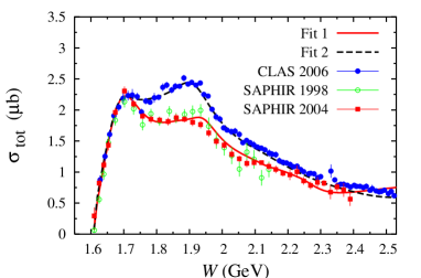
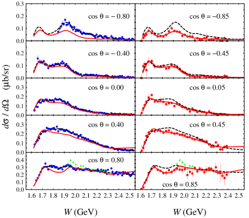
Reference [18] has pointed out that the use of SAPHIR and CLAS data, individually or simultaneously, leads to quite different resonance parameters. This could lead to different conclusions on “missing resonances”, the resonances which have been predicted by constituent quark models but are intangible to $\pi+N\to\pi+N$ reactions that are used by the Particle Data Group (PDG) to extract their properties.

In view of this, the elementary process of kaon production can also be used as a complimentary tool for investigation of the “missing resonances”. As an example, it is worth mentioning the case of “missing” $D_{13}(1895)$ which was observed by Ref. [19] in the $\gamma+p\to K^{+}+\Lambda$ channel. It was found after the previous SAPHIR data [16] showed a clear peak around $W=1900$ MeV in the differential and total cross sections. Subsequently, it was shown in Ref. [20] that the peak could also be equally well reproduced by including a $P_{13}(1950)$ resonance. However, most of analyses based on the isobar model after that confirmed that including the $D_{13}(1895)$ significantly improves the agreement between theoretical prediction and experimental data. Recent partial-wave and coupled-channels analyses confirmed that the peak originates from a $D_{13}$ resonance with a mass around 1900 MeV [21]. Indeed, the same conclusion has also been drawn from the recent multipole study [19], that the peak at $W\sim 1900$ MeV originates from a $D_{13}$ resonance with the extracted mass equals 1936 MeV if SAPHIR data were used or 1915 MeV if CLAS data were used. Thus, future measurements such as the one planned at MAMI in Mainz are, therefore, expected to remedy this unfortunate situation.

2.3 Electromagnetic Production of the Hypertriton

Theoretical calculation of photoproduction of the hypertriton can be done by making use of the left diagram of Fig. 5. The formula for calculating the hypernuclear cross section is similar to the one for calculating the elementary cross sections [cf. Eq. (16)], i.e.,

$$\frac{d\sigma}{d\Omega} = \frac{|\vec{q}|}{|\vec{k}|}~{}\frac{M_{\rm{}^{3}He}E_{\rm{}^{3}_{\Lambda}H}}{32\pi^{2}W^{2}}~{}\sum_{\epsilon}\sum_{M,M^{\prime}}~{}{\textstyle\frac{1}{2}}\left|{\cal T}_{\rm fi}\right|^{2}~{},$$ (17)

except now the nuclear amplitude ${\cal T}_{\rm fi}$ squared is averaged over the initial and final nuclear spins. The nuclear amplitude is somewhat complicated in this case. It consists of the elementary part, integrated over the possible initial and final nucleon momenta and weighted by the nuclear wave functions, and some angular parts in terms of $6j$ and $9j$ coefficients. Explicitly, it is given by

$$T_{\mathrm{f}i} = \sqrt{\frac{6}{\pi}}~{}\sum_{\alpha{\alpha}^{\prime}}~{}\sum_{n\Lambda m_{\Lambda}}i^{n}\hat{n}\hat{{\cal L}}\hat{{\cal S}}\hat{{\cal S}^{\prime}}\hat{\Lambda}(-)^{1+n+{{\cal S}}+M}\delta_{SS^{\prime}}\delta_{LL^{\prime}}\delta_{T0}\times$$ (26)

$$\left(\begin{array}[]{ccc}\frac{1}{2}&\frac{1}{2}&\Lambda\\ M^{\prime}&-M&m_{\Lambda}\end{array}\right)\left\{\begin{array}[]{ccc}{{\cal S}}&{{\cal S}^{\prime}}&n\\ \frac{1}{2}&\frac{1}{2}&1\end{array}\right\}\left\{\begin{array}[]{ccc}{{\cal L}}&{{\cal S}}&\frac{1}{2}\\ L&{{\cal S}^{\prime}}&\frac{1}{2}\\ l&n&\Lambda\end{array}\right\}\times$$

$$\int d^{3}{\vec{q}}~{}p^{2}dp~{}\varphi_{\Lambda}(q\,^{\prime})~{}\Psi_{d}^{(L)}(p)~{}\phi_{\alpha}(p,q)~{}\left[{\bf Y}^{(l)}(\hat{{\vec{q}}\,})\otimes{\bf K}^{(n)}\right]^{(\Lambda)}_{m_{\Lambda}}~{},$$

where the amplitude ${\bf K}^{(n)}$ is related to the elementary amplitude given in Eq. (16) by

$${\cal M}_{\rm fi} = L+i\,{\vec{\sigma}}\cdot{\vec{K}}~{}=~{}\sum_{n=0,1}(-i)^{n~{}}\hat{n}~{}\left[{\bf\sigma}^{(n)}\otimes{\bf K}^{(n)}\right]^{(0)}~{},$$ (27)

with $\sigma^{(n)}$ is the Pauli matrices.

Figure 8: Differential cross section for kaon photoproduction off the proton (dotted line) and ³He (dashed and solid lines) as a function of kaon angle. The dashed line shows the “factorization” approximation for production off the ³He, whereas the solid line represents the exact calculation by using $S$-waves [22]. Solid circle represents the CLAS datum at this kinematic [15].

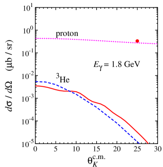
The result is shown in Fig. 8, where we compare the predicted cross sections of hypertriton production with that of elementary reaction. For the hypernuclear production we have performed an exact calculation using Eq. (17) and an approximated one by using the so-called “factorization” approximation. In the latter, the cross section is calculated by means of

$$\frac{d\sigma}{d\Omega} = {\textstyle\frac{1}{6}}~{}W_{A}^{2}~{}|F(Q)|^{2}~{}\left(\frac{d\sigma}{d\Omega}\right)_{\rm elementary}~{},$$ (28)

where $W_{A}$ is a kinematical factor and the “form factor” $F(Q)$ is given by the overlap integral of the two wave functions,

$$F(Q) = \left.\left\langle{}^{3}_{\Lambda}{\rm H}({\vec{p}},{\vec{q}}+{\textstyle\frac{2}{3}}{\vec{Q}})~{}\right|~{}{{}^{3}{\rm He}}({\vec{p}},{\vec{q}})\right\rangle~{}.$$ (29)

Note that in Eq. (29), $\vec{p}$ and $\vec{q}$ denote the momenta of the interacting nucleon and the spectators inside the ${}^{3}{\rm He}$, respectively, whereas $\vec{Q}$ is the momentum transfer (see Fig. 5).

The nuclear cross section at forward angles is smaller than that of elementary kaon production by two orders of magnitude. As $\theta_{K}^{\rm c.m.}$ increases, the cross section drops quickly, since the nuclear momentum transfer increases as a function of $\theta_{K}^{\rm c.m.}$. Since this cross section is in fact very small, photoproduction of hypertriton provides a great challenge to experimentalist. Figure 8 also shows the significant difference between the cross sections calculated with the approximation of Eq. (28) and the full result obtained from Eq. (17). This discrepancy is due to the “factorization” approximation, since in the exact calculation both spin-independent and spin-dependent amplitudes are integrated over the internal momentum and weighted by the two wave functions. This also explains why more structures appear in the cross section of the exact calculation.

Figure 9: Comparison between theoretical calculation and experimental data of the ${}^{3}_{\Lambda}$H (left) and ${}^{4}_{\Lambda}$H (right) electroproduction cross sections. Data are taken from [23].

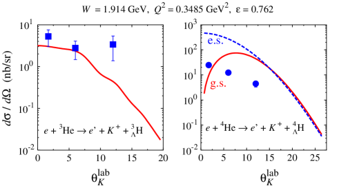
Very recently, Dohrmann et al. [23] measured the electroproduction process on both ³He and ⁴He targets. Although their experiment yielded only three data points in each target, this provides the first evidence on the possibility to produce hypernuclei via electromagnetic process. Our investigation of this process is still in progress. To compare our photoproduction results with these new data, we multiply Eq. (17) with the ratio between the electro- and photoproduction cross sections of the elementary process. The results for both targets are displayed in Fig. 9, where we see that a fair agreement is obtained in the case of the hypertriton production and a significant discrepancy appears for the ⁴He target. This clearly shows that our simple approach urgently requires substantial improvement.

3 Moving to Neutron Star

3.1 Simple Electron and Neutron Stars

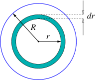
Let us assume that a star has burned all of its “fuel” and the gravitational force starts to contract the star until nothing but the electron degeneracy pressure tries to save the star from a gravitational collapse. To calculate the gravitational pressure, let us consider a solid sphere depicted in Fig. 10. From this figure, it is straightforward to derive the gravitational potential of the shell lying between $r$ and $dr$, which in this case can be written as

$$d{\cal V}_{\rm grav.} = -\frac{G\left(\frac{4}{3}\pi\rho r^{3}\right)\left(4\pi\rho r^{2}dr\right)}{r^{2}}~{}=~{}-\frac{16\pi^{2}\rho^{2}G}{3}\,r^{4}\,dr~{},$$ (30)

where $\rho$ is the density of the sphere and $G$ is the universal gravitational constant. By integrating over the entire radius of the sphere we obtain the total potential energy,

$${\cal V}_{\rm grav.} = -\frac{16\pi^{2}\rho^{2}G}{3}\int_{0}^{R}r^{4}\,dr~{}=~{}-\frac{16\pi^{2}\rho^{2}R^{5}G}{15}~{}=~{}-\frac{3}{5}\,GM^{2}\,\left(\frac{4\pi}{3}\right)^{1/3}V^{-1/3}~{},$$ (31)

where $M$ is the total mass of the sphere and $V$ is its volume. The gravitational pressure is obtained by differentiating Eq. (31) to the volume $V$,

$$p_{\rm grav.} = -\frac{\partial{\cal V}_{\rm grav.}}{\partial V}~{}=~{}-\frac{1}{5}\left(\frac{4\pi}{3}\right)^{1/3}G(Nm_{n})^{2}\,V^{-4/3}~{},$$ (32)

where we have assumed that the sphere contains $N$ neutron each with a mass of $m_{n}$, i.e., $M=Nm_{n}$.

Figure 10: A solid sphere with radius $R$ and density $\rho$. The mass of the shell with the thickness $dr$ is $4\pi\rho r^{2}dr$, whereas the mass of the sphere enclosed by this shell is $4\pi\rho r^{3}/3$.

The degeneracy pressure is obtained from Eq. (9), which can be written as

$$p_{\rm deg.}~{}=~{}\frac{\hbar^{2}\pi^{3}}{15m_{e}}\left(\frac{3N_{e}}{\pi}\right)^{5/3}V^{-5/3}~{},$$ (33)

with $N_{e}$ and $m_{e}$ are the number and the mass of electron.

If there is an equilibrium between the two forces, then we have

$$\frac{1}{5}\left(\frac{4\pi}{3}\right)^{1/3}G(Nm_{n})^{2}\,V^{-4/3} = \frac{\hbar^{2}\pi^{3}}{15m_{e}}\left(\frac{3N_{e}}{\pi}\right)^{5/3}V^{-5/3}~{},$$ (34)

where $N$ and $N_{e}$ are the number of neutron and electron in the star, $m_{n}$ and $m_{e}$ are the neutron and electron masses, respectively. Solving for the star radius, we obtain

$$R = \left(\frac{81\pi^{2}}{128}\right)^{1/3}\frac{\hbar^{2}\pi^{3}}{Gm_{e}m_{n}^{2}}\,N^{-1/3}~{}.$$ (35)

For a star of one solar mass, we have $N\approx 1.2\times 10^{57}$ and assuming $N_{e}=N/2$ we obtain

$$R_{\rm es}~{}\approx~{}1.1\times 10^{4}~{}{\rm km}~{}.$$ (36)

Such a star, for which its collapse is halted by electron degeneracy, is called white dwarf.

However, if we started with a heavier star then the gravitational force would be too strong and the electron degeneracy force could not overcome it. As a consequence, electrons and protons would start the process

$$e^{-}+\,p~{}\to~{}\nu_{e}+\,n~{}.$$ (37)

This process indicates that all atoms in the star start to collapse. Since the neutrino interacts very seldom with other particles, it will exit the star and we are left with a pure neutron star. To calculate the radius of this star we can use Eq. (35) and substitute the mass of electron with the mass of neutron, i.e.,

$$R_{\rm ns} = \left(\frac{81\pi^{2}}{128}\right)^{1/3}\frac{\hbar^{2}\pi^{3}}{Gm_{n}^{3}}\,N^{-1/3}~{}.$$ (38)

If we started with a star with mass equals to the solar mass, we will then end up with a neutron star with $R_{\rm ns}\approx 10$ km. This result should be compared with the solar radius which is approximately $7\times 10^{8}$ km.

3.2 A Slightly More Realistic Neutron Star

The neutron star described in the previous subsection is clearly far from realistic. First of all, because a real neutron star contains not only neutron. Why? Let us consider again the process shown in Eq. (37). Given that a free neutron will decay in about 15 minutes via

$$n~{}\to~{}p~{}+~{}e^{-}+~{}\bar{\nu}_{e}~{},$$ (39)

certain amount of the protons should be present in the neutron star to prevent this weak decay. Most of the energies in the reaction of Eq. (39) is carried away by the anti-neutrino and, therefore, the protons can only occupy the low-energy levels. Once all these levels are filled, Pauli exclusion principle prevents the decay from taking place. On the other hand, the appearance of these protons must be accompanied by the presence of the same amount of electrons, in order to make the charge of the star neutral.

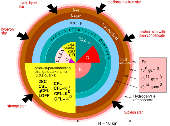
Inside the neutron star the pressure is increasing. As a consequence, other particles such as $\mu,\pi$, and $K$ mesons may appear. Going deeper and deeper we will meet exotic particles, such as $\Lambda,\Sigma,\Xi$, and $\Delta$, or even the up, down, and strange quarks. This can be nicely seen in Fig. 11.

Figure 11: The structure and phase of subatomic matter inside the neutron star as predicted by theory. Also shown in this figure, the density of the crust layers [28] (Courtesy of Prof. Fridolin Weber, San Diego State University).

Besides that, since the pressure is extremely strong, relativistic corrections start to play a significant role. To understand this correction, let us go back to the solid sphere shown in Fig. 10. The gravitational force between the mass of the shell ($dm$) and the mass enclosed by it ($m$) can be written as

$$dF = -\,\frac{G\,m\,dm}{r^{2}}~{}=~{}-\,\frac{G\,m(r)\,\rho(r)\,A(r)\,dr}{r^{2}}~{},$$ (40)

where $\rho(r)$ is the density of the shell and $A(r)$ is the area covered by the shell. By using $dp=dF/A$, we obtain

$$\frac{dp}{dr} = -\,\frac{G\,\rho(r)\,m(r)}{r^{2}}~{}.$$ (41)

We also note that the mass $m(r)$ in Eq. (41) is related to the density $\rho(r)$ by

$$\frac{dm}{dr} = 4\pi\,r^{2}\rho(r)~{}.$$ (42)

Equations (41) and (42) provide the tools to investigate a Newtonian star, i.e., a star for which the mass is not so large and therefore no relativistic correction is needed. These equations can be integrated self consistently, from $r=0$ (where $p=p_{0}$ and $\rho=\rho_{\rm c}$) up to $r=R$ (where $p=0$), to obtain the pressure $p(r)$ and, therefore, the radius $R$ and the mass $M$ of the star. To perform this integration, one needs the information of the matter density $\rho(r)$ in terms of the pressure $p(r)$. This relationship is well known as the equation of state (EOS) of the matter building up the star.

There is a certain class of stars for which the corresponding EOS is quite simple and takes the form

$$p = K\,\rho^{\gamma}~{},$$ (43)

where $K$ is the proportionality constant which depends on the entropy per nucleon and chemical composition. Any star fulfilling Eq. (43) is called a polytrope. The case of polytrope is of interest since there are analytic solutions in terms of Lane-Emden function $\theta(\xi)$ [25]. In this case the radius of the star is given by

$$R = \left[\frac{K\gamma}{4\pi G(\gamma-1)}\right]^{1/2}\rho_{\rm c}^{(\gamma-2)/2}\xi_{1}~{},$$ (44)

whereas its mass is given by

$$M = 4\pi\rho_{\rm c}^{(3\gamma-4)/2}\left[\frac{K\gamma}{4\pi G(\gamma-1)}\right]^{3/2}\xi_{1}^{2}\,\left|\theta^{\prime}(\xi_{1})\right|~{},$$ (45)

where both $\xi_{1}$ and $\theta^{\prime}(\xi_{1})$ are functions of the polytropic index $\gamma$ and tabulated in Ref. [25]. By eliminating $\rho_{\rm c}$ in Eqs. (44) and (45), it can be shown that the relation between mass and radius of this type of star is independent of the choice of $\rho_{\rm c}$.

Most of the known stars can be sufficiently described as Newtonian ones. Besides that, the compact stars known as white dwarfs also fall into this category.

For more massive stars, such as neutron stars, the relativistic correction is needed. This can be performed by multiplying Eq. (41) with three correction factors,

$$\frac{dp}{dr} = -\,\frac{G\,\rho(r)\,m(r)}{r^{2}}\underbrace{\left[1+\frac{p(r)}{\rho(r)c^{2}}\right]\left[1+\frac{4\pi r^{3}p(r)}{m(r)c^{2}}\right]\left[1-\frac{2Gm(r)}{rc^{2}}\right]}_{\rm relativistic~{}corrections}~{},$$ (46)

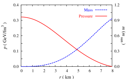
while maintaining the differential equation for $m(r)$ [Eq. (42)]. Equation (46) is known as the Tolman-Oppenheimer-Volkoff (TOV) equation [26]. In this equation the first two factors in square brackets are due to special relativity corrections of order $v^{2}/c^{2}$. It is obvious that these factors go to zero in the limit of $c\to\infty$. The third factor is a general relativity correction. It is also clear that this factor can be neglected in the non-relativistic case. It is obvious from Eq. (46) that an analytic solution of the TOV equation is far from possible. The discussion of the solution to this equation by using an advanced EOS is clearly beyond the scope of this paper. The interested reader can consult Ref. [27] (as well as references therein) for the latest review on this topic. As an example of the numerical solution to the coupled equations (42) and (46) we show the pressure and the mass of neutron star as a function of the distance from the center of the star in Fig. 12. Here, a simple form of the energy density of nuclear matter consisting a compressional term, a symmetry term, and binding energy term, has been used for the corresponding EOS [29].

Figure 12: The pressure and mass of a neutron star calculated from Eqs. (46) and (42) as a function of the distance from its center. In obtaining this result we have used $\rho_{\rm c}=5\rho_{0}$, where $\rho_{0}=0.17~{}{\rm fm}^{-3}$, the normal nuclear density [29].

3.3 Neutrino Mean Free Path in Neutron Stars

In discussing the formation of a neutron star, i.e., Eqs. (37) and (39), we understand that both neutrino and anti-neutrino immediately leave the neutron star as soon as they have been created. Moreover, it is also comprehended that most of the energies coming from the two reactions are carried away by neutrino and anti-neutrino. This has an important consequence in the cooling process of a neutron star, i.e., whereas a conventional body dissipates its energy through photon emissions (electromagnetic radiations), a neutron star cools down via emitting neutrinos and anti-neutrinos.

Therefore, understanding of the interaction between neutrino (as well as anti-neutrino, from now on we will only mention neutrino for the sake of brevity) and neutron star is crucial in the investigation of the neutron star formation. Since the neutron star density is extremely high (see Fig. 11), such interaction is more probable than in the conventional matter. In fact, the neutrino mean free path (the distance between two interactions, from now on called NMFP) could in certain cases be smaller than the diameter of the neutron star. If this happened, we could say that the neutrino is trapped inside the neutron star. The “neutrino trapping” can have a serious consequence in the properties of neutron stars. Indeed, it plays an important role in the supernova explosion or the neutron star cooling process.

Although in the Standard Model massless neutrinos have zero magnetic moment and electronic charge, there are some evidences that neutrino-electron has a magnetic moment ($\mu_{\nu}$) smaller than $1.0\times 10^{-10}\mu_{B}$ at 90% confidence level [30], where $\mu_{B}$ is the Bohr magneton. A stronger bound of $\mu_{\nu}\leq 3.0\times 10^{-12}\mu_{B}$ also exists from astrophysical observation, particularly from the study of the red giant population in globular clusters [31]. On the other hand the neutrino charge radius of $\nu_{e}$ has been estimated from the LAMF experiment [32] to be $R^{2}=(0.9\pm 2.7)\times 10^{-32}~{}{\rm cm}^{2}=(22.5\pm 67.5)\times 10^{-12}~{}{\rm MeV}^{-2}$, while the plasmon decay in the globular cluster star predicts the limit of $e_{\nu}\leq 2\times 10^{-14}\,e$ [31], where $e$ is electron charge.

Figure 13: (Left) The muon-neutrino and muon-antineutrino mean free paths as a function of the ratio between nucleon and nuclear saturation densities. Results for neutrinoless matter are shown in upper panels, whereas results for neutrino trapping with $Y_{l_{e}}$= $0.3$ are shown in lower panels. (Right) Same as in the left panel, but for electron-neutrino and electron-antineutrino [34].

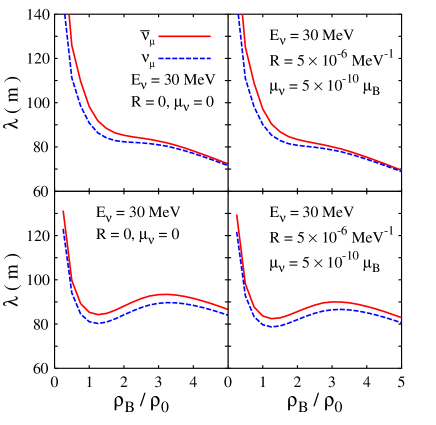
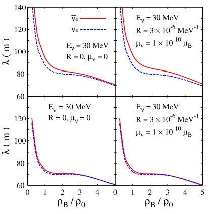
The NMFP (symbolized by ${\lambda}$) is obtained by integrating the cross section of the neutrino-dense-matter interaction over the time- and vector-component of the neutrino momentum transfer,

$$\frac{1}{{\lambda}(E_{{\nu}})}=\int_{q_{0}}^{2E_{{\nu}}-q_{0}}d|{\vec{q}}|\int_{0}^{2E_{{\nu}}}dq_{0}\frac{2{\pi}|{\vec{q}}|}{E^{\prime}_{{\nu}}E_{{\nu}}}~{}\frac{1}{V}\frac{d^{3}{\sigma}}{d^{2}{\Omega}^{\prime}dE^{\prime}_{{\nu}}}~{},$$ (47)

where the cross section for every type of neutrino can be calculated from

$$\frac{1}{V}\frac{d^{3}\sigma}{d^{2}{\Omega}^{\prime}dE^{\prime}_{{\nu}}} = -\frac{G_{F}}{32{\pi}^{2}}\frac{E^{\prime}_{{\nu}}}{E_{{\nu}}}{\rm Im}(L_{{\mu}{\nu}}{\Pi}^{{\mu}{\nu}}).$$ (48)

where $L_{\mu\nu}$ is the neutrino tensor and ${\Pi}^{{\mu}{\nu}}$ is the target polarization tensor, which defines the particle species. Details of the procedure for calculating Eqs. (47) and (48) can be found in Ref. [33]

In order to see the effect more clearly, in this calculation we use relatively large values of neutrino dipole moments and charge radii. Furthermore, besides using conventional matter, we also consider matter with neutrino trapping. The existence of the neutrino in matter allows for the presence of a relatively large number of protons and electrons compared to the case of neutrinoless matter. The appearance of these constituents is then followed by the appearance of a small number of muons at a density larger than two times the nuclear saturation density.

The results for muon-neutrino and electron-neutrino mean free paths are shown in Fig. 13, where we chose the neutrino energy $E_{\nu}=30$ MeV. From this figure it is obvious that in the case of neutrinoless matter, contribution from the neutrino charge radius is too small compared to that from the nucleon weak magnetism. On the other hand, in the case of neutrino trapping, but with zero muon-neutrino dipole moment and charge radius, the difference in the neutrino and antineutrino mean free paths is significant, especially at high densities. Although almost similar to the neutrinoless matter case, contribution from the neutrino charge radius is very small, and therefore it is invisible in this kinematics. It is also apparent that in both cases for densities around $(2-3)\rho_{0}$, $\lambda_{\nu}$ and $\lambda_{\bar{\nu}}$ behave differently, i.e., if neutrinos are present in matter, the mean free paths increase the density, but if neutrinos are absent, the opposite phenomenon is observed. We have shown that this result is more pronounced at higher neutrino energies [34].

Figure 14: Total differential cross sections as functions of the momentum transfer $q^{\mu}=(q_{0},\vec{q}_{1})$ for the case where neutrinos are trapped with $Y_{l_{e}}=0.3$ and baryon density $\rho_{B}=5\rho_{0}$, while $E_{\nu}=5$ MeV [35].

In the case of electron-neutrino, although the effect is less significant for neutrinoless matter at high densities, contribution from the neutrino charge radius yields an enhancement to the difference between $\lambda_{\nu}$ and $\lambda_{\bar{\nu}}$. On the contrary, for the case of zero neutrino dipole moment and charge radius, but with neutrino trapping, the difference of neutrino and antineutrino mean free paths is suppressed. Thus for this kind of matter, we may conclude that the neutrino charge radius does not contribute to the mean free path difference.

Another alternative to study the properties of the neutrino-dense matter interaction is by investigating the sensitivity of the corresponding differential cross section to these possibly nonzero neutrino electromagnetic properties. The result for the case of neutrino trapping with leptonic fraction $Y_{l_{e}}=0.3$ and baryon density $\rho_{B}=5\rho_{0}$ is shown in Fig. 14, where we plot the total differential cross sections as functions of the time- and vector-component of the four-momentum transfer $q^{\mu}$.

From Fig. 14 we can clearly see that the cross section magnitude is quite sensitive to the neutrino electromagnetic properties. Including contribution from the neutrino magnetic moment and charge radius leads to a cross section which is 14 times larger than that of point neutrino. It is also apparent that most of this contribution come from the neutrino charge radius, whereas the different shape in the $q_{1}$ distribution is mainly driven by the neutrino magnetic moment.

We have also compared this result to the case of neutrinoless matter [35]. We found that, in general, neutrino trapping enhances the magnitude of the cross section, as we expected, since matter with neutrino trapping contains more protons and, hence, electromagnetic interactions are more likely to occur. If we switched off the neutrino electromagnetic properties, this behavior clearly disappears.

3.4 Critical Density of Dense Matter

From Fig. 11 it is apparent that a neutron star is expected to have a solid inner crust above its liquid mantle. The mass of this crust has been known to be sensitively dependent on the density of the inner edge and on the EOS. Therefore, investigation of the dynamical instability of dense matter will certainly shed important information on the inner structure of neutron stars.

Figure 15: Critical densities of different RMF models as a function of the neutrino fraction in matter.

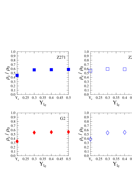
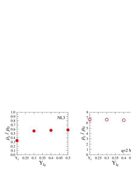
Recent investigations on this topic have disclosed that the critical density ($\rho_{c}$), a density at which the uniform liquid becomes unstable to a small density fluctuation, can be used as a good approximation of the edge density of the crust [36]. The important aspects of their finding are that the inner edge of the crust density to be $\rho_{\rm edge}=0.08~{}{\rm fm^{-3}}$ and a measurement of the neutron radius in the ${}^{208}{\rm Pb}$ nucleus will provide useful information on the $\rho_{c}$.

To this end we have investigated the behavior of the predicted critical density ($\rho_{c}$) in matter with and without neutrino trapping for several different relativistic mean field (RMF) models [37]. The ratio between the critical density and the normal nuclear density as a function of the neutrino fraction in matter is shown in Fig. 15 for several different RMF models.

It is found that different treatments in the isovector-vector sector of RMF models yield more substantial effects in matter without neutrino trapping than in matter with neutrino trapping. Moreover, for matter with neutrino trapping, the value of $\rho_{c}$ does not significantly change with the variation of the models nor with the variation of the neutrino fraction in matter. In this case, the value of $\rho_{c}$ is larger for matter with neutrino trapping. These effects are due to the interplay between the major role of matter composition and the role of the effective masses of mesons and nucleons.

It is also found that the additional nonlinear terms of Horowitz-Piekarewicz and Effective RMF models can prevent another instability at relatively high densities from appearing. This can be traced back to the effective $\sigma$ mass, which goes to zero when the density approaches $6.5\rho_{0}$.

4 Connecting What We Have Learned So Far

So far, we have discussed hypernucleus and neutron star starting from the Pauli exclusion principle. We know that the important ingredient of a hypernucleus is hyperon, whereas the basic building block of a neutron star is neutron. According to their symmetry, both neutron and hyperon are classified in the SU(3) baryon octet. We have also implicitly built an argument that without this principle we know nothing about the physics of hypernuclear and neutron star.

Now, we can nicely connect hyperon, neutron, hypernucleus, and neutron star as shown in Fig. 16. Starting from this figure, we may ask: what can be constructed based on our knowledge about them? A tentative answer is also shown in this figure.

Figure 16: Connecting and extending from what we have learned so far.

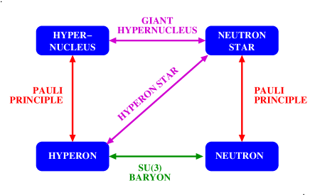
Within the RMF model, the question whether a neutron star could be considered as a giant hypernucleus has been asked more than 20 years ago [38]. Earlier discussion which showed that the existence of hyperon in neutron star is plausible has been done based on Fermi gas model [39]. For our current discussion this would not be too difficult to understand if we look back at Fig. 11, where we can clearly see that at certain density (depth) there is a $\Lambda$ population. In fact, Glendenning has found that this population starts to grow at baryon density $\rho_{B}\approx 0.4~{}{\rm fm}^{-1}$ and starts to dominate all star ingredients at $\rho_{B}\approx 0.9~{}{\rm fm}^{-1}$ [38]. Such population is found in the cores of the relatively heavier neutron stars and is about 15%–20% of the total baryon population.

We can continue the discussion to the hyperon stars as well as quark stars. They are indeed more massive, more complicated, and more interesting than the neutron star. However, we have to stop this discussion here, otherwise I have the feeling that our experimentalist colleagues would complain that we, theoreticians, are too imaginative and too creative. Could this be true? The next section could convince you that this could be true.

5 Econophysics, are Theoreticians too Creative?

5.1 Why Econophysics?

The scientific challenge to understand the nature of complex systems is too tempting to the physicists. Some of them have been fascinated by the huge, and also growing, amount of economics data recorded minutes by minutes for decades. Among these interesting data, the fluctuation of stock exchange indices is of special interest, since it might indirectly reflect the economic situation in a certain region. Furthermore, the advancement in computing capabilities has enabled us to handle this large amount of data, unlike the situation almost 40 years ago, when Mandelbrot investigated approximately 2000 data points of cotton prices [40].

It is said that such studies could explain the nature of interacting elements in the complex systems and, therefore, could help to forecast economic fluctuations in the future. In other words, these studies were intended to produce new results in economics, which might help us to avoid economic “earthquakes” such as what happened in Indonesia several years ago [41].

5.2 Time Series Analysis

We start our analysis with an investigation of the daily index returns, which are defined as

$$Z_{\Delta t}(t) = \ln Y(t+\Delta t)-\ln Y(t)~{}=~{}\ln\,[Y(t+\Delta t)/Y(t)],$$ (49)

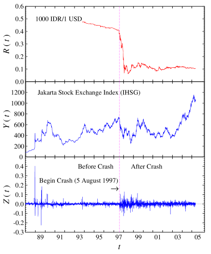
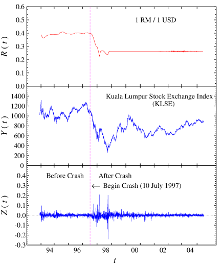
where $Y(t)$ indicates the closing index of the stock at day $t$. We use the time series data from two different stock indices, the Jakarta Stock Exchange Index (abbreviated with IHSG, an acronym of Indeks Harga Saham Gabungan or the composite stock exchange price index) and the Kuala Lumpur Stock Exchange index (KLSE), which belong to different countries. Comparing the two indices would be very interesting since both Indonesia and Malaysia underwent the same monetary crisis in 1997, which was then followed by financial crashes in almost all economic sectors, but with quite different economic situations.

Figure 17 shows the time series of the IHSG and KLSE indices along with their logarithmic returns calculated by using Eq. (49). For comparison, in this figure (top panels) we also display the historical time series of the exchange rate of Indonesian Rupiah and Malaysian Ringgit, since the economic crashes started with the devastating decline of these rates. It is obvious from this figure that the fluctuation $Y(t)$ of both indices is more dramatic than that of S&P 500, indicating that in this case the situation is far more complex. After the crash the magnitude of returns $Z(t)$ is significantly larger in both indices, or, in the economics language, the probability to gain or to loose becomes larger than before.

Figure 17: (Left) The ratio between 1000 Indonesian Rupiah and 1 US Dollar (top), the Jakarta Stock Exchange Index (IHSG) $Y(t)$ (middle) and the logarithmic return $Z(t)$ calculated from Eq. (49) as a function of time $t$ sampled with $\Delta t=1$ day (bottom). (Right) The ratio between 1 Malaysian Ringgit and 1 US Dollar (top), the Kuala Lumpur Stock Exchange Index (KLSE) $Y(t)$ (middle) and the logarithmic return $Z(t)$ (bottom) as a function of time sampled for $\Delta t=1$ day. On 1st September 1998 Malaysia imposed currency controls, the Ringgit was pegged with US Dollar with a fixed rate of 3.80 Ringgit per Dollar. The arrows in the bottom panels indicate the time position when the IHSG and KLSE started to crash. Data are taken from Ref. [42] (IDR/USD and RM/USD exchange rates) Ref. [43] (IHSG stock index), and Ref. [44] (KLSE stock index).

Figure 18: Number of the returns given by Eq. (49) that exceeds one up to seven standard deviations ($\sigma$) for the IHSG (top panel) and the corresponding derivatives at $1\sigma$ (lower panel).

5.3 Omori Law, from Geophysics to Finance Physics

To accurately determine the time position of the crash we make use of the Omori law. Omori law, which was originally used in geophysics [45], states that the number of aftershock earthquakes per unit time measured at time $t$ after the main earthquake decays as a power law. Practically it is written as

$$n(t) = K\,(t+\tau)^{-p}~{},$$ (50)

where $K$ and $\tau$ are two positive constants. The cumulative number of aftershocks is obtained by integrating Eq. (50) from 0 to $t$, i.e.,

$$N(t) = \int_{0}^{t}dt^{\prime}\,K(t^{\prime}+\tau)^{-p}~{}=~{}\frac{K\left[(t+\tau)^{1-p}-\tau^{1-p}\right]}{1-p}~{}.$$ (51)

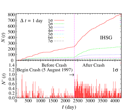
This number is found to be more relevant to compare with the presently analyzed data. By calculating the number of returns given by Eq. (49) that exceeds one standard deviation ($\sigma$) up to $7\sigma$, we arrive at Fig. 18 for the IHSG case. From this figure we can clearly see that there exists a discontinuity on 5 August 1997, which indicates the start of a crash process. To exactly find the position of this discontinuity we calculate the first derivative of $N(t)$ for $N(t)$ obtained with $1\sigma$, shown in the lower panels of Fig. 18. From these three panels we are convinced that the IHSG started its crash process on 5 August 1997. The same procedure has been also applied to the KLSE index, from which we obtain that the KLSE started to crash on 10 July 1997, almost one month before the IHSG case. The crash positions of the two indices are indicated by the vertical lines in Fig. 17.

Figure 19: (Left) Log-log plots of the IHSG probability of return to the origin as a function of the sampling time $\Delta t$ before and after crash. Solid lines are obtained from linear regressions to this probability. The slopes of these lines, which are equal to negative inverse of the Lévy stable distribution indices, are shown in the left panels. Comparison between normalized distribution functions for $\Delta t=1$ and normalized Lévy stable distributions with parameters obtained from the left figures is shown in the second column panels. The standard deviation and the number of data used are also shown in these panels. (Right) Same as in the four left panels, but for the KLSE case before and after crash.

Figure 20: Moments of the distribution of the IHSG (top) and KLSE (bottom) normalized returns, before (left panel) and after (right panel) crash, given in Eq. (55) for $\Delta t=1,2,3,4,6,9,13$, and 19 days compared with those obtained from the Gaussian distribution (solid thick lines).

5.4 Probability Density Function

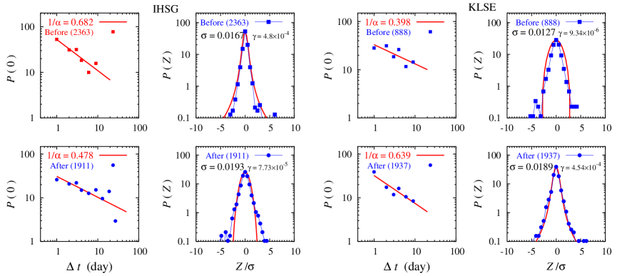
Following previous studies [46, 47] we investigate the probability density function [PDF or $P(Z)$] of the return to the origin $P(0)$ in order to investigate the statistical properties of both indices. The advantage of using such analysis is that we can reduce the statistical inaccuracies, since the number of data included is relatively small, whereas the probability is largest at $Z=0$.

Starting with the characteristic function [47]

$$\varphi(\Delta t)~{}=~{}e^{-\gamma\Delta t|q|^{\alpha}}~{},$$ (52)

the Lévy stable distribution is given by

$$P(Z)~{}=~{}\frac{1}{\pi}\,\int_{0}^{\infty}\,e^{-\gamma\Delta t|q|^{\alpha}}\cos(qZ)\,dq~{}.$$ (53)

From Eq. (53) the probability of return to the origin $P(0)$ reads

$$P(0)~{}=~{}\frac{\Gamma(1/\alpha)}{\pi\alpha(\gamma\Delta t)^{1/\alpha}}~{},$$ (54)

where $\Gamma$ indicates the Gamma function.

The log-log plots of $P(0)$ as a function of the sampling time $\Delta t$ for both IHSG and KLSE indices are shown in the first and third column panels of Fig. 19. The slopes of linear regressions to these plots equal the negative inverse of the Lévy stable distribution indices $\alpha$. Using this index we calculate the parameter $\gamma$ by means of Eq. (54) and plot the “theoretical” PDF as a function of normalized returns $Z/\sigma$, using Eq. (53), where $\sigma$ is the standard deviation of the distribution, and compare it with the empirical PDF obtained from data in Fig. 19. Figure 19 reveals the fact that in the case of IHSG the distribution turns from Lévy to Gaussian after the crash. Surprisingly, the KLSE stock index shows a contrary result, the distribution alters from a Gaussian to a Lévy one after the crash.

5.5 Distribution Moment

It has been argued that the use of the return probability to the origin ${\rm PDF}(0)$ to estimate the Lévy stable distribution index $\alpha$ is statistically not optimal, due to discreteness of the distribution [48]. Instead of exploiting such method, a different strategy has been proposed, i.e. by calculating $\alpha$ by means of the slope of the cumulative distribution tails in a log-log plot. To further test their results on the scaling behavior, Refs. [48, 49] analyzed the moments of the distribution of normalized returns

$$\mu(k)~{}=~{}\langle\,|g(t)|^{k}\rangle~{}.$$ (55)

where the normalized returns $g(t)$ is defined by

$$g(t)~{}=~{}\frac{Z(t)-\langle Z(t)\rangle}{\sqrt{\langle Z^{2}(t)\rangle-\langle Z(t)\rangle^{2}}}~{},$$ (56)

with $\langle Z(t)\rangle$ the time average of $Z(t)$ over the entire of time series. In the case of the S&P 500 index the result is found to be consistent with the analysis of the tails of cumulative distributions. References [48, 49] pointed out that the change in the moments behavior originates from the gradual disappearance of the Lévy slope in the distribution tails. In our case it is also important to cross-check the result shown in Fig. 19, since the number of data used in this analysis is significantly smaller than that of previous analysis on the S&P 500 index, e.g. Ref. [48], which used approximately $5\times 10^{6}$ data points.

It has been also shown in Ref. [48] that Eq. (55) will diverge for $k\geq 3$. In this study we also constrain $k$ within $0\leq k\leq 3$. The results for both indices compared with the moment obtained from a Gaussian distribution have been reported in Ref. [50]. It is found that the IHSG moment retains its scaling up to $\Delta t=9$ days, only after $\Delta t=13$ the moment starts to deviate toward the Gaussian distribution. In the KLSE case the moment quickly converges to the Gaussian distribution as soon as $\Delta t$ increases from 1 day and does not show any scaling behavior as in the former case.

In Fig. 20 we display the moments of both stock indices in the case of before and after the financial crash. A consistent result, compared to the analysis of Fig. 19, is obtained from Fig. 20, i.e., in the case of IHSG the distribution becomes closer to Gaussian after crash, whereas the KLSE moments move away from the Gaussian distribution after the crash.

Another important finding obtained from Fig. 20 is that the scaling behavior up to $\Delta t=9$ shown by the IHSG case in the previous section originates from the “before crash” period. After the crash, the IHSG moments quickly converge to a Gaussian distribution. In fact, this phenomenon has already been seen in the left panels of Fig. 19, where the empirical probability of return to the origin is more scattered after crash.