Primordial Evolution in the Finitary Process Soup

Abstract

A general and basic model of primordial evolution—a soup of reacting finitary and discrete processes—is employed to identify and analyze fundamental mechanisms that generate and maintain complex structures in prebiotic systems. The processes—$\epsilon$-machines as defined in computational mechanics—and their interaction networks both provide well defined notions of structure. This enables us to quantitatively demonstrate hierarchical self-organization in the soup in terms of complexity. We found that replicating processes evolve the strategy of successively building higher levels of organization by autocatalysis. Moreover, this is facilitated by local components that have low structural complexity, but high generality. In effect, the finitary process soup spontaneously evolves a selection pressure that favors such components. In light of the finitary process soup’s generality, these results suggest a fundamental law of hierarchical systems: global complexity requires local simplicity.

I Introduction

The very earliest stages of evolution—or rather, pre-evolution—remain a mystery. How did structure emerge in a system of simple interacting objects, such as molecules? How was this structure commandeered as substrate for subsequent evolution—evolution that continued to transform the objects themselves? One wonders if this recursive interplay between structure and dynamics facilitated the emergence of complex and functional organizations. Since these questions concern the most fundamental properties of evolutionary systems, we explore them using principled and rigorous methods.

To build a suitable model a few basic ingredients are required. First, one needs some type of elementary objects that constitute the state of the system at its finest resolution. Second, one needs rules for how the objects interact. Third, one needs an environment in which the objects interact. Fourth, one needs quantitative and calculable notions of structure and organization. These requirements led us to the finitary process soup model of primordial evolution [1]. Simply stated, the soup’s ingredients are, in order, $\epsilon$-machines, their functional composition, a flow reactor, and the structural complexity $C_{\mu}$ of $\epsilon$-machines.

After explaining each of these ingredients, we will relate the model to classical replicator dynamics by reducing the soup to a special case. We then move on to contrast the limited case with the full-fledged finitary process soup as a constructive, unrestricted dynamical system.

II Objects: $\epsilon$-machines

Here we employ a finite-memory process called an $\epsilon$-machine [2, 3, 4], as our preferred representation of an evolving information-processing individual. Using a population of $\epsilon$-machines is particularly appropriate in studying self-organization and evolution from an information-theoretic perspective as they allow quantitative measurements of storage capacity and randomness. Rather than using the abstraction of a formal language—an arbitrary finite set of finite length words—we consider a discrete-valued, discrete-time stationary stochastic process described by a bi-infinite sequence of random variables $S_{t}$ over an alphabet $\mathcal{A}$:

$$\stackrel{{\scriptstyle\leftrightarrow}}{{S}}=...S_{1}S_{0}S_{1}....$$ (1)

A process stores information in a set of causal states that are equivalence classes of semi-infinite histories that condition the same probability distribution for future states. More formally, the causal states $\boldsymbol{{\cal S}}$ of a process are the members of the range of the map $\epsilon:~{}{\stackrel{{\scriptstyle\leftarrow}}{{\rm{\bf S}}}}\mapsto 2^{{\stackrel{{\scriptstyle\leftarrow}}{{\rm{\bf S}}}}}$ from histories to sets of histories:

$$\epsilon({\stackrel{{\scriptstyle\leftarrow}}{{s}}})=\{{{\stackrel{{\scriptstyle\leftarrow}}{{s}}}}^{\prime}|{\rm P}(\stackrel{{\scriptstyle\rightarrow}}{{S}}|\stackrel{{\scriptstyle\leftarrow}}{{S}}={\stackrel{{\scriptstyle\leftarrow}}{{s}}})~{}={\rm P}(\stackrel{{\scriptstyle\rightarrow}}{{S}}|\stackrel{{\scriptstyle\leftarrow}}{{S}}={{\stackrel{{\scriptstyle\leftarrow}}{{s}}}}^{\prime})\}~{},$$ (2)

where $2^{{\stackrel{{\scriptstyle\leftarrow}}{{\rm{\bf S}}}}}$ denotes the power set of ${\stackrel{{\scriptstyle\leftarrow}}{{\rm{\bf S}}}}$. Further, let ${\cal S}\in\boldsymbol{{\cal S}}$ be the current casual state, ${\cal S}^{\prime}$ its successor, and ${\stackrel{{\scriptstyle\rightarrow}}{{S}}}^{1}$ the next symbol in the sequence (1). The transition from one causal state ${\cal S}_{i}$ to another ${\cal S}_{j}$ that emits the symbol $s\in\mathcal{A}$ is given by a set of labeled transition matrices: $\boldsymbol{\cal T}=\{T_{ij}^{(s)}:s\in\mathcal{A}\}$, where

$$T_{ij}^{(s)}\equiv{\rm P}({\cal S}^{\prime}={\cal S}_{j},{\stackrel{{\scriptstyle\rightarrow}}{{S}}}^{1}=s|{\cal S}={\cal S}_{i}).$$ (3)

The $\epsilon$-machine of a process is the ordered pair $\{\boldsymbol{{\cal S}},\boldsymbol{\cal T}\}$. One can show that it is the minimal, maximally predictive causal representation of the process [4]. Unlike a general probabilistic $\epsilon$-machine, for simplicity, here we take causal-state transitions to have equal probabilities. The finitary $\epsilon$-machines can be thought of as finite-state machines with a certain properties [4]: (1) All states are start states and accepting states; (2) All recurrent states form a single strongly connected component; (3) All transitions are deterministic: A causal state together with the next value observed from the process determines a unique next causal state; And (4) the set of causal states is minimal. Here we use an alphabet of input and output pairs over a binary alphabet: $\mathcal{A}=\{0|0,0|1,1|0,1|1\}$. This implies that the $\epsilon$-machines work as mappings between sets of strings. In other words, they are transducers [5].

Figure 1: Three examples of $\epsilon$-machines. $T_{A}$ represents the identity function and has the causal state $A$. $T_{B}$ has two causal states ($A$ and $B$), accepts the input string $1010\ldots$ or $0101\ldots$, and operates by flipping $0$s to $1$s and vice versa. $T_{C}$ has the same domain and range as $T_{B}$, but maps input strings onto themselves.

In contrast to prior models of pre-biotic evolution, $\epsilon$-machines are simply finitely-specified mappings. More to the point, they do not have two separate modes of representation (information storage) or functioning (transformation). The advantage is that there is no assumed distinction between gene and protein [6, 7] or between data and program [8, 9, 10, 11]. Instead, one recovers the dichotomy by projecting onto (i) the sets that an $\epsilon$-machine recognizes and generates and (ii) the mapping between these sets. Examples of $\epsilon$-machines are shown in Figure 1.

III Interaction: functional composition

The basic pairwise interaction we use in the finitary process soup is functional composition. Two machines interact and produce a third machine—their composition. Composition is not a symmetric operation. Machine $T_{A}$ composed with another $T_{B}$ does not necessarily result in the same machine as $T_{B}$ composed with $T_{A}$: $T_{B}\circ T_{A}\neq T_{A}\circ T_{B}$.

The upper bound on the number of states of the composition is the product of the number of states of the parents: $|T_{B}\circ T_{A}|\leq|T_{B}|\times|T_{A}|$. Hence, there is the possibility of exponential growth of states and machine complexity if machines are iteratively composed. A composition, though, may also result in a machine with lower complexity than those of its parents.

III.1 Interaction networks

We represent the interactions among a set of $\epsilon$-machines with an interaction network $\mathcal{G}$ which is a a graph whose nodes correspond to $\epsilon$-machines and whose transitions correspond to interactions. If $T_{k}=T_{j}\circ T_{i}$ occurs in the soup, then the edge from $T_{i}$ to $T_{k}$ is labeled $T_{j}$. One may represent $\mathcal{G}$ with the binary matrices:

$$\mathcal{G}_{ij}^{(k)}=\begin{cases}1&\text{if $T_{k}=T_{j}\circ T_{i}$}\\ 0&\text{otherwise}.\end{cases}$$ (4)

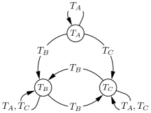
Consider the $\epsilon$-machines in Fig. 1, for example. They are related via composition according to the interaction graph shown in Fig. 2, which is given by the matrices

$$\mathcal{G}^{(A)}=\left[\begin{matrix}1&0&0\\ 0&0&0\\ 0&0&0\end{matrix}\right]~{},$$ (5)

$$\mathcal{G}^{(B)}=\left[\begin{matrix}0&1&0\\ 1&0&1\\ 0&1&0\end{matrix}\right]~{},$$ (6)

and

$$\mathcal{G}^{(C)}=\left[\begin{matrix}0&0&1\\ 0&1&0\\ 1&0&1\end{matrix}\right].$$ (7)

Figure 2: Interaction network of the $\epsilon$-machines in Fig. 1. There is a transition, for example, that is labeled $T_{C}$ from the node $T_{A}$ to the node $T_{C}$, since $T_{A}$ composed with $T_{C}$ results in $T_{C}$ (in fact, each transition from $T_{A}$ has the same label as the label of its respective sink node since $T_{A}$ is the identity function).

III.2 Meta-machines

For a machine to survive in its environment somehow it needs to produce copies of itself. This can be done directly by self-reproduction, e.g. $T_{A}\circ T_{A}=T_{A}$, or it can be done indirectly in cooperation with other machines: e.g., $T_{A}$ facilitates the production of $T_{B}$, which facilitates the production of $T_{C}$, which, in turn, closes the loop by facilitating the production of $T_{A}$. In other words, there can be sets of machines that interact with each other in such a way that they collectively self-reinforce the overall production of the set. This leads to the notion of an autonomous and self-replicating entity, which we call a meta-machine. Inspired by Maturana and Varela’s autopoietic set [12], Eigen and Schuster’s hypercycle [13], and Fontana and Buss’ organization [14], we define a meta-machine $\Omega$ to be a connected set of $\epsilon$-machines whose interaction matrix consists of all and only the members of the set. That is, a set $\Omega$ is a meta-machine if and only if (1) the composition of two $\epsilon$-machines from the set is always itself a member of the set:

$$T_{j}\circ T_{i}\in\Omega,~{}~{}\forall T_{i},T_{j}\in\Omega~{};$$ (8)

(2) all $\epsilon$-machines in the set can arise from the composition of two machines in the set:

$$\exists T_{i},T_{j}\in\Omega,~{}~{}T_{k}=T_{j}\circ T_{i},~{}~{}\forall T_{k}\in\Omega~{};$$ (9)

and (3) there is a nondirected path between every pair of nodes in $\Omega$’s interaction network $\mathcal{G}_{\Omega}$. The third property ensures that there is no subset of $\Omega$ that is isolated from the rest of $\Omega$ under composition. Consider, for example, the union of two self-replicators, $T_{A}$ and $T_{B}$, for which $T_{B}\circ T_{A}=T_{A}\circ T_{B}=T_{\emptyset}$. According to property (3), they are not a meta-machine.

IV Complexity measures: $C_{\mu}$

In previous computational pre-biotic models, the objects have been represented by, for example, assembly language codes [8, 9, 10, 11], tags [15, 16], $\lambda$-expressions [17] and cellular automata [18]. We employ $\epsilon$-machines instead mainly for one reason: there is a well developed theory (computational mechanics) of their structural properties. Assembly language programs and $\lambda$-expressions, for instance, are computational universal representations and so one knows that it is not possible to calculate their complexity [5].

For finitary $\epsilon$-machines, in contrast, complexity can be readily defined and analytically calculated in closed form. Define the stochastic connection matrix of an $\epsilon$-machine $M=\{\boldsymbol{{\cal S}},\boldsymbol{\cal T}\}$ as $\mathbf{T}\equiv\sum_{s\in\mathcal{A}}T^{(s)}$. The probability distribution $p_{\boldsymbol{{\cal S}}}$ over the states in $\boldsymbol{{\cal S}}$—how often they are visited—is given by the normalized left eigenvector of T associated with eigenvalue $1$.

The structural complexity $C_{\mu}$ of $M$ is the Shannon entropy of the distribution given by $p_{\boldsymbol{{\cal S}}}$,

$$C_{\mu}(M)\equiv\sum_{v\in\boldsymbol{{\cal S}}}p_{\boldsymbol{{\cal S}}}^{(v)}\log_{2}p_{\boldsymbol{{\cal S}}}^{(v)}.$$ (10)

The structural complexity of an $\epsilon$-machine is the amount of information stored in the distribution over $\boldsymbol{{\cal S}}$, which is the minimum average amount of memory needed to optimally predict future configurations [4].

To measure the diversity of interactions in the soup we define the interaction network complexity $C_{\mu}(\mathcal{G})$ to be the Shannon entropy of the distribution of effective transition probabilities in the graph $\mathcal{G}$. We consider, in particular, only the transitions that have occurred between machine types that are present. That is,

$$C_{\mu}(\mathcal{G})\equiv\sum_{p_{i,j,k}\neq 0}{\upsilon_{ij}^{k}\log_{2}\upsilon_{ij}^{k}},$$ (11)

where

$$\upsilon_{ij}^{k}=\begin{cases}p_{i}p_{j}/\sum{\upsilon_{ij}^{k}}&\text{if $T_{k}=T_{j}\circ T_{i}$ has occurred}\\ 0&\text{otherwise.}\end{cases}$$ (12)

and $p_{i}$ is the fraction of machines of type $i$ in the population. To monitor the emergence of actual and functional reproduction paths, we consider only those interactions that occurred in the population.

V Framework: the soup

Figure 3: A schematic illustration of the finitary process soup. Two $\epsilon$-machines, $T_{A}$ and $T_{B}$, are composed and produce a third machine $T_{C}$, or a random machine $T_{R}$ is introduced to the soup. In either case, another randomly selected machine $T_{D}$ is removed to maintain a fixed population size. Note that this is a well stirred setting, and so there is no spatial relationship in the population.

The $\epsilon$-machines interact in a well stirred reactor with the following iterated dynamics:

1. Production and influx:

   1. With probability $\Phi_{in}$ generate a random $\epsilon$-machine $T_{R}$.

   2. With probability $1-\Phi_{in}$ (reaction):

      1. Select $T_{A}$ and $T_{B}$ randomly.

      2. Form the composition $T_{C}=T_{B}\circ T_{A}$.

2. Outflux:

   1. Select an $\epsilon$-machine $T_{D}$ randomly from the population.

   2. Replace $T_{D}$ with the $\epsilon$-machine produced in the previous step—either $T_{C}$ or $T_{R}$.

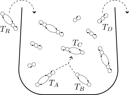
$T_{R}$ is uniformly sampled from the set of all two-state $\epsilon$-machines in our simulations (see below). This sampling is also used when initializing the population. The insertion of $T_{R}$ corresponds to an influx while the removal of $T_{D}$ corresponds to an outflux. The latter keeps the population size constant. See Fig. 3 for a schematic illustration. There is no spatial dependence in this version of the soup as $\epsilon$-machines are sampled uniformly from the population for each replication and removal.

VI Closed population dynamics

To familiarize ourselves with the model we first examine a simple base case: a soup with no influx that is initialized with machines taken from a finite set which is closed under composition. This case is also intended to work as a bridge between classical population dynamics and the general, constructive dynamics of the finitary process soup. The closure with respect to composition enables us to describe the system’s temporal dynamics of $\epsilon$-machine concentrations by a coupled system of ordinary differential equations. In the limit of an infinite soup size, the rate equation of concentration $p_{k}$ of machine type $T_{k}$ is given by

$$\dot{p}_{k}=\psi_{k}-\Phi_{out}p_{k},\ \ k=1,...,n,$$ (13)

where the conditional production rate $\psi_{k}$ is the probability that $T_{k}$ is produced given that two randomly sampled machines are paired:

$$\psi_{k}=\sum_{i,j=1}^{n}{\alpha_{ij}^{k}p_{i}p_{j}},$$ (14)

and $\alpha_{ij}^{k}$ is a second-order reaction rate constant:

$$\alpha_{ij}^{k}=\begin{cases}1&\text{if $T_{k}=T_{j}\circ T_{i}$}\\ 0&\text{otherwise.}\end{cases}$$ (15)

The outflux $\Phi_{out}$ equals the total production rate of the soup—i.e., the probability that a reaction occurs given that two $\epsilon$-machines are paired. It keeps the size of the soup constant:

$$\Phi_{out}(t)=\sum_{i=1}^{n}{\psi_{i}}.$$ (16)

Given a soup with no influx, $\Phi_{in}=0$, that hosts machines which are members of a set that is closed under composition, the distribution dynamics can alternatively be predicted from by its interaction network:

$$\mathbf{p}_{t}^{(k)}=\mathbf{p}_{t-1}\cdot\mathcal{G}_{ij}^{(k)}\cdot\mathbf{p}_{t-1}^{T}Z^{-1},$$ (17)

where $\mathbf{p}_{t}^{(k)}$ is the frequency of $\epsilon$-machine type $k$ at time $t$ and $Z^{-1}$ is a normalization factor. This approximates the soup’s elements as updating synchronously.

We illustrate the closed case by initiating the soup with machines that consist of only a single state—mono-machines. There are 15 mono-machines, the null (transition-less) transducer is excluded, and they form a closed set under composition. See Fig. 4 for the temporal dynamics of their respective frequencies. Nine machine types remain in the population at equilibrium. They form a meta-machine $\mathcal{M}$ with $C_{\mu}(\mathcal{M})=5.75$ bits. In this case, since $C_{\mu}(T_{i})=0$ for all mono-machines $T_{i}$, the population’s structural complexity derives only from its interaction network.

Figure 4: A simple base case: Machine type frequencies of mono-machines as functions of time. $N$ $(=100,000)$ denotes the population size. Dashed lines: simulation; solid lines: Eq. (17).

VII Open population dynamics

We now move on to the general case of a soup with positive influx rate consisting of $\epsilon$-machines  of arbitrary size. The soup then constitutes a constructive dynamical system where there is a mutual dependence between its equations of motion and the individuals. Due to the openness, Eqs. (13)-(17) do not necessarily apply. We therefore turn to simulations.

In order to study dynamics that is ruled solely by compositional transformations we first set the influx rate to zero. A fine-grained description of the soup’s history on the $\epsilon$-machine level is given by a genealogy—a record of descent of machine types. By studying the example in Fig. 5, a simulation with $N=100$ individuals, one important observation is that nearly all the $\epsilon$-machine types that are present in the soup’s initial population are replaced over time. Thus, genuine novelty emerges, in contrast to the closed soup just described. Initially, there is a rapid innovation phase in which novel machines are introduced that displace the bulk of the initial machines. The degree of innovation flattens out, along with the diversity of the soup, and eventually vanishes as the population becomes increasingly closed under composition.

Figure 5: Genealogy of $\epsilon$-machine types in a soup with 100 machines. A solid line denotes that a machine type is present in the soup. Dashed lines (drawn from the parents to the child) denote composition. Note that almost the the whole set of initial $\epsilon$-machine types (with one exception) is replaced by the dynamics.

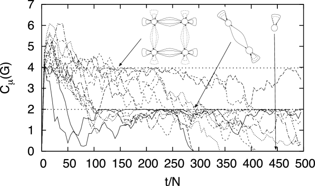
To monitor the soup’s organization over time, we superimpose $C_{\mu}(\mathcal{G})$ time series from several runs in Fig. 6. One sees that plateaus are formed. These can be explained in terms of meta-machines. In addition to capturing the notion of self-replicating entities, meta-machines also describe an invariant set of the population dynamics. That is, formally,

$$\Omega=\mathcal{G}\circ\Omega,$$ (18)

where $\Omega$ is the set of $\epsilon$-machines present in the population and $\mathcal{G}$ is their interaction network. These invariant sets can be stable or unstable under the population dynamics.

Consider, for example, the meta-machine in Fig. 2. It is unstable, since $T_{A}$s are only produced by $T_{A}$s, and will decay over time to the meta-machine of Fig. 7. This also illustrates, by the way, how trivial self-replication is spontaneously attenuated in the soup.

Figure 6: Decomposition of meta-machines in a soup with no influx. Superimposed plots of $C_{\mu}(\mathcal{G})$ from 15 separate runs with $N=500$. $C_{\mu}(\mathcal{G})$ is bounded by 4 bits while a 4-element meta-machine (shown), denoted $\Omega_{4}$, is the largest one in the soup. $\Omega_{4}$ decays to $\Omega_{2}$, a 2-element meta-machine (shown) due to fluctuations, that in turn decays to $\Omega_{1}$, a single self-reproducing $\epsilon$-machine.

Figure 7: The resulting meta-machine when the meta-machine in Fig. 2 decays under the population dynamics of Eq. (17).

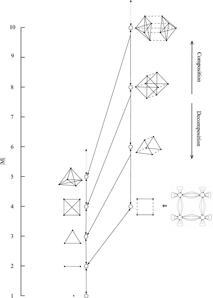
The plateaus at $C_{\mu}(\mathcal{G})=4$ bits, $C_{\mu}(\mathcal{G})=2$ bits, and $C_{\mu}(\mathcal{G})=0$ bits correspond to the largest meta-machine that is present at that time. Since a meta-machine by definition is closed under composition, it itself does not produce novel machines; thus, one has the upper bound of $C_{\mu}(\mathcal{G})$. As a meta-machine is reduced due to an internal instability or sampling fluctuations by the outflux, the upper bound of $C_{\mu}(\mathcal{G})$ is lowered. This results in a stepwise and irreversible succession of meta-machine decompositions. Fig. 6 shows only three plateaus. In principle, however, there is one plateau for every meta-machine that at some point is the largest one in the population. The diagram in Fig. 8 summarizes our results from a more systematic survey of spontaneously generated meta-machine hierarchies in simulations of soups with 500 $\epsilon$-machines.

Figure 8: Composition and decomposition hierarchy of meta-machines. Dots denote self-replicating $\epsilon$-machines, solid lines denote $T_{A}\stackrel{{\scriptstyle T_{B}}}{{\longrightarrow}}T_{C}$ transitions and dashed lines denote equivalent $T_{B}\stackrel{{\scriptstyle T_{A}}}{{\longrightarrow}}T_{C}$ transitions. The label of the source node and the transition label are interchanged in the latter transition type. This results in a redundant representation of the interaction network, which is used to show how the meta-machines are related. The interaction networks are shown in a simplified way according to $\Omega_{4}$; cf. Fig. 6.

(a)

(b)

Figure 9: (a) Population- and run-averaged $\epsilon$-machine complexity $\langle C_{\mu}(T)\rangle$ and (b) run-averaged interaction network complexity $\langle C_{\mu}(\mathcal{G})\rangle$ as a function of time $t$ and influx rate $\Phi_{in}$ for a population of $N=100$ objects. (Reprinted with permission from [1]).

We now examine the effects of influx by studying the population-averaged $\epsilon$-machine complexity $\langle C_{\mu}(T)\rangle$ and the run-averaged interaction network complexity $\langle C_{\mu}(\mathcal{G})\rangle$ as a function of $t$ and $\Phi_{in}$, see Fig. 9.

The average $\epsilon$-machine complexity $\langle C_{\mu}(T)\rangle$ increases rapidly initially before declining to a steady state. The average interaction network complexity $\langle C_{\mu}(\mathcal{G})\rangle$ is relatively high where the average structural complexity of the $\epsilon$-machines is low, and is maximized at $\Phi_{in}\approx 0.1$. Higher influx rates have a destructive effect on the populations’ interaction network due to the new individuals’ low reproduction rate. $\langle C_{\mu}(T)\rangle$ is, in contrast, maximized at a relatively high influx rate ($\Phi_{in}\approx 0.75$) at which $\langle C_{\mu}(\mathcal{G})\rangle$ is relatively small. The maximum network complexity $\widehat{C_{\mu}}(\mathcal{G})$ of the population grows linearly at a positive rate of approximately $7.6\cdot 10^{-4}$ bits per replication.

VIII Discussion

We presented a conceptual model of pre-biotic evolution: a soup consisting of objects that make new objects [1]. The objects are $\epsilon$-machines and they generate new $\epsilon$-machines by functional composition. The soup constitutes a constructive dynamical system since the population dynamics is not fixed and may itself evolve along with the state space it operates on. Specifically, the dimension of the state space changes over time, which is reminiscent of the constructive population dynamics associated with punctuated equilibria [19].

In principle, this allows for open-ended evolution. The quantitative estimate quoted above for the linear growth of the interaction network complexity supports this intriguing possibility occurring in the open finitary process soup. In the case of no influx, though, the system reaches a steady state where the soup consists of only one self-replicator. Growth and maintenance of organizational complexity requires that the system is dissipative; i.e., that there is a small, but steady inflow of random $\epsilon$-machines. Notably, in this case, the soup spontaneously evolves hierarchical organizations in the population—meta-machines that in turn are organized hierarchically.

These hierarchies are assembled from noncomplex, general individual $\epsilon$-machines. In this way, the soup’s emergent complexity derives largely from a network of interactions, rather than from the unbounded increase in the structural complexity of individuals. It appears, therefore, that higher-order complex organization not only allows for simple local components but, in fact, requires them.