Dyson Indices and Hilbert-Schmidt Separability Functions and Probabilities

Abstract

A confluence of numerical and theoretical results leads us to conjecture that the Hilbert-Schmidt separability probabilities of the 15- and 9-dimensional convex sets of complex and real two-qubit states (representable by $4\times 4$ density matrices $\rho$) are $\frac{8}{33}$ and $\frac{8}{17}$, respectively. Central to our reasoning are the modifications of two ansätze, recently advanced (Phys. Rev. A, 75 [2007], 032326), involving incomplete beta functions $B_{\nu}(a,b)$, where $\nu=\frac{\rho_{11}\rho_{44}}{\rho_{22}\rho_{33}}$. We, now, set the separability function $\mathcal{S}_{real}(\nu)$ proportional to $B_{\nu}(\nu,\frac{1}{2},2)=\frac{2}{3}(3-\nu)\sqrt{\nu}$. Then, in the complex case—conforming to a pattern we find, manifesting the Dyson indices ($\beta=1,2,4$) of random matrix theory–we take $\mathcal{S}_{complex}(\nu)$ proportional to $\mathcal{S}_{real}^{2}(\nu)$. We also investigate the real and complex qubit-qutrit cases. Now, there are two variables, $\nu_{1}=\frac{\rho_{11}\rho_{55}}{\rho_{22}\rho_{44}},\nu_{2}=\frac{\rho_{22}\rho_{66}}{\rho_{33}\rho_{55}}$, but they appear to remarkably coalesce into the product $\eta=\nu_{1}\nu_{2}=\frac{\rho_{11}\rho_{66}}{\rho_{33}\rho_{44}}$, so that the real and complex separability functions are again univariate in nature.

Mathematics Subject Classification (2000): 81P05, 52A38, 15A90, 81P15

I Introduction

Życzkowski and Sommers have derived—using random matrix theory (in particular, the Laguerre ensemble)—general formulas for the $(n^{2}-1)$-dimensional and the
$\frac{n(n+1)-2}{2}$-dimensional volumes of the complex and real $n\times n$ density matrices ($\rho$), respectively, in terms of the Hilbert-Schmidt (HS) metric Życzkowski and Sommers (2003) (Bengtsson and Życzkowski, 2006, sec. 14.3) (as well as the Bures metric (Bengtsson and Życzkowski, 2006, sec. 14.4) Sommers and Życzkowski (2003); Slater (2005a)). Later, Andai Andai (2006) examined these and related questions, using a quite different framework. He applied mathematical induction on the leading principal minors of $\rho$, along with the established formulas for hyperareas of surfaces of $n$-spheres and beta integrals. He reproduced—up to normalization factors—the HS real and complex volume formulas in Życzkowski and Sommers (2003) (and, moreover, the $(2n^{2}-n-1)$-dimensional quaternionic volumes). (In addition to the HS and Bures metrics, Andai considered, for the single qubit case, the broad [infinitely nondenumerable] class—which does include the Bures as its minimal member—of monotone metrics. Unlike Życzkowski and Sommers, he did not obtain formulas for the hyperareas occupied by density matrices of less than full rank.)

Despite these considerable theoretical advances, volume (and, hence, probability) formulas have not yet become available for the important subsets of separable ($n\leq 6$) and positive-partial-transpose ($n\geq 8$) $n\times n$ density matrices ($n$ composite). (Szarek Szarek (2005) employed methods of asymptotic convex geometry to estimate the volume of the set of separable mixed quantum states for $N$ qubits, and Aubrun and Szarek Aubrun and Szarek for $N$ qudits. It was concluded in these studies that the separable volumes were superexponentially small in the dimension of the set of states. For large $D$, the $(D^{2}-1)$-dimensional volume for bipartite systems of positive-partial-transpose states, however, is much larger than the volume of separable states (Aubrun and Szarek, , Thm. 4).)

To address this fundamental lacuna, at least in the Hilbert-Schmidt context (cf. Slater (a)), we developed in Slater (2007) a methodology—incorporating the Bloore parameterization of density matrices Bloore (1976) (sec. I.1). Its numerical application led to ansätze, involving (apparently independent) incomplete beta functions, for the 9-dimensional real and 15-dimensional complex separable volumes in the qubit-qubit ($n=4$) case Slater (2007). In the sequel to that study here, we, first, apply this Bloore framework to various scenarios involving $n\times n$ density matrices ($n=4,6,8,9$), in which certain of their off-diagonal entries have been nullified. This enables us to now obtain exact results, of interest in themselves, and possibly suggestive of solutions/approaches to the full (non-nullified) highly computationally-challenging problems.

In fact, based on certain (real-complex-quaternionic) patterns emerging in these exact results (sec. II.1.4), bearing an obvious relation to the Dyson indices ($\beta=1,2,4$) of random matrix theory Dyson (1970), we are led to modify the incomplete beta function ansätze for the two full (real and complex) problems advanced in Slater (2007). The “separability function” in the complex case is now not analyzed as if it were independent of that in the real case (which we still take to be an incomplete—but slightly different—beta function), but actually simply proportional to its square. These central analyses will be elaborated upon in sec. IX, (eqs. (94) - (96)), where it shown that the modified ansätze do, in fact, accord well (Fig. 3) with the numerical results of Slater (2007).

We begin our extensive series of lower-dimensional analyses, by examining a number of two-qubit scenarios (sec. II). In them, we are able to compute a number of interesting exact two-qubit scenario-specific HS separability probabilities. (Listing them in increasing order, we have $\left\{\frac{1}{10},\frac{1}{3},\frac{3}{8},\frac{2}{5},\frac{135\pi}{1024},\frac{16}{3\pi^{2}},\frac{3\pi}{16},\frac{5}{8},\frac{105\pi}{512},2-\frac{435\pi}{1024},\frac{11}{16},1\right\}$.) For each of the scenarios, we identify a certain univariate separability function $\mathcal{S}_{scenario}(\nu)$, where $\nu=\frac{\rho_{11}\rho_{44}}{\rho_{22}\rho_{33}}$. The integral over $\nu\in[0,\infty]$ of the product of this function (typically of a piecewise nature over [0,1] and $[1,\infty]$) with a scenario-specific (marginal) jacobian function $\mathcal{J}_{scenario}(\nu)$ yields the HS separable volume ($V^{HS}_{sep}$). The ratio of $V^{HS}_{sep}$ to the HS total (entangled and non-entangled) volume ($V^{HS}_{tot}$) gives us the HS scenario-specific separability probability.

The question of the “relative proportion” of entangled and non-entangled states in a given generic class of composite quantum systems, had apparently first been raised by Życzkowski, Horodecki, Sanpera and Lewenstein (ZHSL) in a much-cited paper Życzkowski et al. (1998). They gave “three main reasons”—“philosophical”, “practical” and “physical”—upon which they expanded, for pursuing the topic. The present author, motivated by the ZHSL paper, has investigated this issue in a number of settings, using various (monotone and non-monotone) measures on quantum states, and a variety of numerical and analytical methods Slater (2000a, 1999, b, 2002, b, 2005b, 2005a, 2006) (cf. Szarek et al. (2006); Gurvits and Barnum (2002, 2003, )). Though the problems are challenging (high-dimensional) in nature, many of the results obtained in answer to the ZHSL question in these various contexts have been strikingly simple and elegant (and/or conjecturally so).

Specifically here, we further develop the (Bloore-parameterization-based) approach presented in Slater (2007). This was found to be relatively effective in studying the question posed by ZHSL, in the context of two-qubit systems (the smallest possible example exhibiting entanglement), endowed with the (non-monotone Ozawa (2000)) Hilbert-Schmidt (HS) measure Życzkowski and Sommers (2003), inducing the flat, Euclidean geometry on the space of $4\times 4$ density matrices. This approach Slater (2007) exploits two distinct features of a form of density matrix parameterization first discussed by Bloore Bloore (1976). These properties allow us to deal with lower-dimensional integrations (more amenable to computation) than would otherwise be possible. We further find that the interesting advantages of the Bloore parameterization do, in fact, carry over—in a somewhat modified fashion—to the qubit-qutrit (sec. III and X.1), qutrit-qutrit (sec. IV) and qubit-qubit-qubit (secs. V and VI) domains.

I.1 Bloore (off-diagonal-scaling) parameterization

We, first, consider the 9-dimensional convex set of (two-qubit) $4\times 4$ density matrices with real entries, and parameterize them—following Bloore Bloore (1976) (cf. (Kurowicka and Cooke, 2003, p. 235))—as

$$\rho=\left(\begin{array}[]{llll}\rho_{11}&z_{12}\sqrt{\rho_{11}\rho_{22}}&z_{13}\sqrt{\rho_{11}\rho_{33}}&z_{14}\sqrt{\rho_{11}\rho_{44}}\\ z_{12}\sqrt{\rho_{11}\rho_{22}}&\rho_{22}&z_{23}\sqrt{\rho_{22}\rho_{33}}&z_{24}\sqrt{\rho_{22}\rho_{44}}\\ z_{13}\sqrt{\rho_{11}\rho_{33}}&z_{23}\sqrt{\rho_{22}\rho_{33}}&\rho_{33}&z_{34}\sqrt{\rho_{33}\rho_{44}}\\ z_{14}\sqrt{\rho_{11}\rho_{44}}&z_{24}\sqrt{\rho_{22}\rho_{44}}&z_{34}\sqrt{\rho_{33}\rho_{44}}&\rho_{44}\end{array}\right).$$ (1)

One, of course, has the standard requirements that $\rho_{ii}\geq 0$ and (the unit trace condition) $\Sigma_{i}\rho_{ii}=1$. Now, three additional necessary conditions (which can be expressed without using the diagonal entries, due to the $\rho_{ii}\geq 0$ stipulation) that must be fulfilled for $\rho$ to be a density matrix (with all eigenvalues non-negative) are: (1) the non-negativity of the determinant (the principal $4\times 4$ minor),

$$\left(z_{34}^{2}-1\right)z_{12}^{2}+2\left(z_{14}\left(z_{24}-z_{23}z_{34}\right)+z_{13}\left(z_{23}-z_{24}z_{34}\right)\right)z_{12}-z_{23}^{2}-z_{24}^{2}-z_{34}^{2}+$$ (2)

$$+z_{14}^{2}\left(z_{23}^{2}-1\right)+z_{13}^{2}\left(z_{24}^{2}-1\right)+2z_{23}z_{24}z_{34}+2z_{13}z_{14}\left(z_{34}-z_{23}z_{24}\right)+1\geq 0;$$

(2): the non-negativity of the leading principal $3\times 3$ minor,

$$-z_{12}^{2}+2z_{13}z_{23}z_{12}-z_{13}^{2}-z_{23}^{2}+1\geq 0;$$ (3)

and (3): the non-negativity of the principal $2\times 2$ minors (although actually only the $i=j=1$ case is needed, it is natural to impose them all),

$$1-z_{ij}^{2}\geq 0.$$ (4)

As noted, the diagonal entries of $\rho$ do not enter into any of these constraints—which taken together are sufficient to guarantee the nonnegativity of $\rho$ itself—as they can be shown to contribute only (cancellable) non-negative factors to the determinant and principal minors. This cancellation property is certainly a principal virtue of the Bloore parameterization, allowing one to proceed analytically in lower dimensions than one might initially surmise. (Let us note that, utilizing this parameterization, we have been able to establish a recent conjecture of Månsson, Porta Mana and Björk regarding Bayesian state assignment for three-level quantum systems, and, in fact, verify our own four-level analogue of their conjecture (Månsson et al., a, eq. (52)) Månsson et al. (b).)

Additionally, implementing the Peres-Horodecki condition Peres (1996); Horodecki et al. (1996); Bruß and Macchiavello (2005) requiring the non-negativity of the partial transposition of $\rho$, we have the necessary and sufficient condition for the separability (non-entanglement) of $\rho$ that (4):

$$\nu\left(z_{34}^{2}-1\right)z_{12}^{2}+2\sqrt{\nu}\left(\nu z_{13}z_{14}+z_{23}z_{24}-\sqrt{\nu}\left(z_{14}z_{23}+z_{13}z_{24}\right)z_{34}\right)z_{12}-z_{23}^{2}-\nu z_{34}^{2}+\nu+$$ (5)

$$+\nu\left(\left(z_{24}^{2}-1\right)z_{13}^{2}-2z_{14}z_{23}z_{24}z_{13}-z_{24}^{2}+z_{14}^{2}\left(z_{23}^{2}-\nu\right)\right)+2\sqrt{\nu}\left(z_{13}z_{23}+\nu z_{14}z_{24}\right)z_{34}\geq 0,$$

where

$$\nu=\mu^{2}=\frac{\rho_{11}\rho_{44}}{\rho_{22}\rho_{33}},$$ (6)

being the only information needed, at this stage, concerning the diagonal entries of $\rho$. (It is interesting to contrast the role of our variable $\nu$, as it pertains to the determination of entanglement, with the rather different roles played by the concurrence and negativity Verstraete et al. (2001a); Iwai (2007).) We have vacillated between the use of $\nu$ and $\mu$ as our principal variable in our two previous studies Slater (c, 2007). In sec. VII, we will revert to the use of $\mu$, as it appears that its use can avoid the appearances of square roots, which, it is our impression, at least, can impede certain Mathematica computations.

I.1.1 Reduction of dimensionality

Thus, the Bloore parameterization is evidently even further convenient here, in reducing the apparent dimensionality of the separable volume problem. That is, we now have to essentially consider only the separability variable $\nu$ rather than three independent (variable) diagonal entries. (This supplementary feature had not been commented upon by Bloore, as he discussed only $2\times 2$ and $3\times 3$ density matrices, and also, obviously, since the Peres-Horodecki separability condition had not yet been formulated in 1976.) The (two variable—$\nu_{1},\nu_{2}$) analogue of (6) in the $6\times 6$ (qubit-qutrit) case will be discussed and implemented in sec. III. Additionally still, we find a four-variable counterpart in the $9\times 9$ qutrit-qutrit instance [sec. IV], and three-variable counterparts in two sets of qubit-qubit-qubit analyses (secs. V and VI). (The question of whether any or all of these several ratio variables are themselves observables would seem to be of some interest.) It certainly appears to us that in the qubit-qutrit case (sec. III and X.1) the two associated ratio variables ($\nu_{1},\nu_{2}$) importantly merge or coalesce into the simple product $\eta=\nu_{1}\nu_{2}$ for all analytical purposes. (Products of ratio variable do also appear in the limited number of still higher-dimensional analyses we report below, so perhaps some similar merging or coalescing takes place in those settings, as well.)

In (Slater, 2007, eqs. (3)-(5)), we expressed the conditions (found through application of the “cylindrical algebraic decomposition” Brown (2001)) that—in terms of the Bloore variables $z_{ij}$’s—an arbitrary 9-dimensional $4\times 4$ real density matrix $\rho$ must fulfill. These took the form,

$$z_{12},z_{13},z_{14}\in[-1,1],z_{23}\in[Z^{-}_{23},Z^{+}_{23}],z_{24}\in[Z^{-}_{24},Z^{+}_{24}],z_{34}\in[Z^{-}_{34},Z^{+}_{34}],$$ (7)

where

$$Z^{\pm}_{23}=z_{12}z_{13}\pm\sqrt{1-z_{12}^{2}}\sqrt{1-z_{13}^{2}},Z^{\pm}_{24}=z_{12}z_{14}\pm\sqrt{1-z_{12}^{2}}\sqrt{1-z_{14}^{2}},$$ (8)

$$Z^{\pm}_{34}=\frac{z_{13}z_{14}-z_{12}z_{14}z_{23}-z_{12}z_{13}z_{24}+z_{23}z_{24}\pm s}{1-z_{12}^{2}},$$

and

$$s=\sqrt{-1+z_{12}^{2}+z_{13}^{2}-2z_{12}z_{13}z_{23}+z_{23}^{2}}\sqrt{-1+z_{12}^{2}+z_{14}^{2}-2z_{12}z_{14}z_{24}+z_{24}^{2}}.$$ (9)

I.1.2 Possible transformations of the $z_{ij}$’s

In his noteworthy paper, Bloore also presented (Bloore, 1976, secs. 6,7) a quite interesting discussion of the “spheroidal” geometry induced by his parameterization. This strongly suggests that it might prove useful to reparameterize the $z_{ij}$ variables in terms of spheroidal-type coordinates. Following the argument of Bloore—that is, performing rotations of the $(z_{13},z_{23})$ and $(z_{14},z_{24})$ vectors by $\frac{\pi}{4}$ and recognizing that each pair of so-transformed variables lay in ellipses with axes of length $\sqrt{1\pm z_{12}}$—we were able to substantially simply the forms of the feasibility conditions ((7)-(9)).

Using the set of transformations (having a jacobian equal to $\frac{\left(1-z_{12}^{2}\right)\gamma_{1}}{2\gamma_{2}}$)

$$z_{13}\to\frac{\left(\sqrt{1-z_{12}}\cos\left(\theta_{1}\right)+\sin\left(\theta_{1}\right)\sqrt{z_{12}+1}\right)\sqrt{\gamma_{1}\gamma_{2}+1}}{\sqrt{2}},$$ (10)

$$z_{23}\to\frac{\left(\sin\left(\theta_{1}\right)\sqrt{z_{12}+1}-\cos\left(\theta_{1}\right)\sqrt{1-z_{12}}\right)\sqrt{\gamma_{1}\gamma_{2}+1}}{\sqrt{2}},$$

$$z_{14}\to\frac{\left(\sqrt{1-z_{12}}\cos\left(\theta_{2}\right)+\sin\left(\theta_{2}\right)\sqrt{z_{12}+1}\right)\sqrt{\gamma_{1}+\gamma_{2}}}{\sqrt{2}\sqrt{\gamma_{2}}},$$

$$z_{24}\to\frac{\left(\sin\left(\theta_{2}\right)\sqrt{z_{12}+1}-\cos\left(\theta_{2}\right)\sqrt{1-z_{12}}\right)\sqrt{\gamma_{1}+\gamma_{2}}}{\sqrt{2}\sqrt{\gamma_{2}}},$$

$$z_{34}\to Z_{34}-\frac{\cos\left(\theta_{1}-\theta_{2}\right)\sqrt{\gamma_{1}+\gamma_{2}}\sqrt{\gamma_{1}\gamma_{2}+1}}{\sqrt{\gamma_{2}}},$$

one is able to replace the conditions ((7)-(9)) that the real two-qubit density matrix $\rho$—given by (1)—must fulfill by

$$\gamma_{1}\in[0,1];\hskip 7.22743pt\gamma_{2}\in[\gamma_{1},\frac{1}{\gamma_{1}}];\hskip 7.22743ptZ_{34}\in[-\gamma_{1},\gamma_{1}];\hskip 7.22743ptz_{12}\in[-1,1];\hskip 7.22743pt\theta_{1},\theta_{2}\in[0,2\pi].$$ (11)

We developed this set of transformations at a rather late stage of the research reported here, and presently have no indications that are of any special aid in regard to the particular difficulties/challenges posed by the HS separability-probability question. So, the qubit-qubit results reported below (sec. II) do rely essentially upon the conditions ((7)-(9)) and the original parameterization in terms of the $z_{ij}$’s of Bloore.

Another very interesting simplifying parameterization—expressed in terms of correlations and partial correlations—can be found in the statistical/mathematical literature Kurowicka and Cooke (2003, 2006a, 2006b); Joe (2006); Makhoul (1990). (In fact, the Bloore parameterization can be readily seen—in retrospect—to be simply a way of decomposing a density matrix into a correlation matrix (cf. de Vicente ), plus its diagonal entries.) But this too seems to have no particular enhanced value in analyzing partial transposes. (The cited literature also appears to be highly relevant to the problem of the random generation of density matrices.)

I.2 Previous analysis and beta function ansätze

In Slater (2007), we studied the four nonnegativity conditions (as well as their counterparts —having completely parallel cancellation and univariate function properties—in the 15-dimensional case of $4\times 4$ density matrices with, in general, complex entries) using numerical (primarily quasi-Monte Carlo integration) methods. We found a close fit to the function (Slater, 2007, Figs. 3, 4),

$$\mathcal{S}^{approx}_{real}(\nu)=\left(4+\frac{1}{5\sqrt{2}}\right)B\left(\frac{1}{2},\sqrt{3}\right)^{8}B_{\nu}\left(\frac{1}{2},\sqrt{3}\right),$$ (12)

entering into our formula (cf. (17), (18)),

$$V^{HS}_{sep/real}=2\int_{0}^{1}\mathcal{J}_{real}(\nu)\mathcal{S}_{real}(\nu)d\nu=\int_{0}^{\infty}\mathcal{J}_{real}(\nu)\mathcal{S}_{real}(\nu)d\nu,$$ (13)

for the 9-dimensional Hilbert-Schmidt separable volume of the real $4\times 4$ density matrices (Slater, 2007, eq. (9)). Here, $B$ denotes the (complete) beta function, and $B_{\nu}$ the incomplete beta function Gupta and Nadarajah (2004),

$$B_{\nu}(a,b)=\int_{0}^{\nu}w^{a-1}(1-w)^{b-1}dw.$$ (14)

Additionally (Slater, 2007, eq. (10)),

$$\mathcal{J}_{real}(\nu)=\frac{\nu^{3/2}\left(12\left(\nu(\nu+2)\left(\nu^{2}+14\nu+8\right)+1\right)\log\left(\sqrt{\nu}\right)-5\left(5\nu^{4}+32\nu^{3}-32\nu-5\right)\right)}{3780(\nu-1)^{9}}$$ (15)

is the (apparently highly oscillatory near $\nu=1$ (Slater, 2007, Fig. 1)) jacobian function resulting from the transformation to the $\nu$ variable of the Bloore jacobian $(\Pi_{i=1}^{4}\rho_{ii})^{\frac{3}{2}}$. (A referee did indicate that the apparent oscillations vanished, when he employed a Maple program using 50 digits of precision. [Only in the latest Version 6 of Mathematica is a comparable plot feasible.] Also, perhaps, we should refer to $\mathcal{J}_{real}(\nu)$ as a marginal jacobian, since it is the result of the integration of a three-dimensional jacobian function over two, say $\rho_{11}$ and $\rho_{22}$, variables.)

In the 15-dimensional complex two-qubit case, we found that the function

$$S^{approx}_{complex}(\nu)=\left(\frac{100000000}{2\sqrt[3]{2}+\frac{10^{3/4}}{3^{2/3}}}\right)B\left(\frac{2\sqrt{6}}{5},\frac{3}{\sqrt{2}}\right)^{14}B_{\nu}\left(\frac{2\sqrt{6}}{5},\frac{3}{\sqrt{2}}\right),$$ (16)

provided a close fit to our numerical results (Slater, 2005b, eq. (14)).

I.3 Research design and objectives

Although we were able to implement the three (six-variable) nonnegativity conditions ((2), (3) and (4)) exactly in Mathematica in Slater (2007), for density matrices of the form (1), we found that additionally incorporating the fourth Peres-Horodecki (separability) one (5)—even holding $\nu$ fixed at specific values—seemed to yield a computationally intractable problem.

In light of the apparent computational intractability in obtaining exact results in the 9-dimensional real (and a fortiori 15-dimensional complex) two-qubit cases, we adjusted the research program pursued in Slater (2007). We now sought to determine how far we would have to curtail the dimension (the number of free parameters) of the two-qubit systems in order to be able to obtain exact results using the same basic investigative framework. Such results—in addition to their own intrinsic interest—might help us understand those previously obtained (basically numerically) in the full 9-dimensional real and 15-dimensional complex cases Slater (2007) (which, retrospectively, in fact, we assert does turn out to be the case).

To pursue this lower-dimensional exact strategem, we nullified various $m$-subsets of the six symmetrically-located off-diagonal pairs in the 9-parameter real density matrix (1), and tried to exactly implement the so-reduced non-negativity conditions ((2), (3), (4) and (5))—both the first three (to obtain HS total volumes) and then all four jointly (to obtain HS separable volumes). We leave the four diagonal entries themselves alone in all our analyses, so if we nullify $m$ pairs of symmetically-located off-diagonal entries, we are left in a (9-m)-dimensional setting. We consider the various combinatorially distinct scenarios individually, though it would appear that we also could have grouped them into classes of scenarios equivalent under local operations, and simply analyzed a single representative member of each equivalence class.

We will be examining a number of scenarios of various dimensionalities (that is, differing numbers of variables parameterizing $\rho$). In all of them, we will seek to find the univariate function $\mathcal{S}_{scenario}(\nu)$ (our primary computational and theoretical challenge) and the constant $c_{scenario}$, such that

$$V^{HS}_{sep/scenario}=\int_{0}^{\infty}\mathcal{S}_{scenario}(\nu)\mathcal{J}_{scenario}(\nu)d\nu,$$ (17)

and

$$V^{HS}_{tot/scenario}=c_{scenario}\int_{0}^{\infty}\mathcal{J}_{scenario}(\nu)d\nu.$$ (18)

Given such a pair of volumes, one can immediately calculate the corresponding HS separability probability,

$$P^{HS}_{sep/scenario}=\frac{V^{HS}_{sep/scenario}}{V^{HS}_{tot/scenario}}.$$ (19)

Let us note that in the full 9-dimensional real and 15-dimensional complex two-qubit cases recently studied in Slater (2007), it was quite natural to expect that $\mathcal{S}_{real}(\nu)=\mathcal{S}_{real}(\frac{1}{\nu})$ (and $\mathcal{S}_{complex}(\nu)=\mathcal{S}_{complex}(\frac{1}{\nu})$). But, here, in our lower-dimensional scenarios, the nullification of entries that we employ, breaks symmetry (duality), so we can not realistically expect such a reciprocity property to hold, in general. Consequently, we adopt the more general, broader formula in (13) as our working formula (17).

We now embark upon a series of multifarious lower-dimensional analyses, first for qubit-qubit and then qubit-qutrit, qutrit-qutrit and qubit-qubit-qubit systems. These will prove useful—as was our original hope—in developing approaches to higher-dimensional analyses, presently out of the reach of exact computer analyses.

II Qubit-Qubit Analyses

To begin, let us make the simple observation that since the partial transposition operation on a $4\times 4$ density matrix interchanges only the (1,4) and (2,3) entries (and the (4,1) and (3,2) entries), any scenario which does not involve at least one of these entries must only yield separable states.

II.1 Five nullified pairs of off-diagonal entries—6 scenarios

II.1.1 4-dimensional real case—$P^{HS}_{sep}=\frac{3\pi}{16}$

There are, of course, six ways of nullifying five of the six off-diagonal pairs of entries of $\rho$. Of these, only two of the six yield any non-separable (entangled) states. In the four trivial (fully separable) scenarios, the lower-dimensional counterpart to $\mathcal{S}_{real}(\nu)$ was of the form $\mathcal{S}_{scenario}(\nu)=c_{scenario}=2$.

In one of the two non-trivial scenarios, having the (2,3) and (3,2) pair of entries of $\rho$ left intact (not nullified), the separability function was

$$\mathcal{S}_{[(2,3)]}(\nu)=\begin{cases}2\sqrt{\nu}&0\leq\nu\leq 1\\ 2&\nu>1.\end{cases}$$ (20)

(It is of interest to note that $B_{\nu}(\frac{1}{2},1)=2\sqrt{\nu}$, while in Slater (2007), we had conjectured that $\mathcal{S}_{real}(\nu)$ was proporitional to $B_{\nu}(\frac{1}{2},\sqrt{3})$.)

In the other non-trivial scenario, with the (1,4) and (4,1) pair being the one not nullified, the separability function was—in a dual manner (mapping $f(\nu)$ for $\nu\in[0,1]$ into $f(\frac{1}{\nu})$ for $\nu\in[1,\infty]$)—equal to

$$\mathcal{S}_{[(1,4)]}(\nu)=\begin{cases}2&0\leq\nu\leq 1\\ \frac{2}{\sqrt{\nu}}&\nu>1.\end{cases}$$ (21)

In both of these scenarios (having $c_{scenario}=2$) for the total (separable and non-separable) HS volume, we obtained $V^{HS}_{tot}=\frac{\pi}{48}\approx 0.0654498$ and $V^{HS}_{sep}=\frac{\pi^{2}}{256}\approx 0.0385531$. The corresponding HS separability probability for the two non-trivial (dual) scenarios is, then, $\frac{3\pi}{16}\approx 0.589049$.

II.1.2 5-dimensional complex case—$P^{HS}_{sep}=\frac{1}{3}$

Now, we allow the single non-nullified pair of symmetrically-located entries to be complex in nature (so, obviously we have five variables/parameters—that is, including the three diagonal variables—in toto to consider, rather than four).

Again, we have only the same two scenarios (of the six combinatorially possible) being separably non-trivial. Based on the (2,3) and (3,2) pair of entries, the relevant function (with the slight change of notation to indicate complex entries) was

$$\mathcal{S}_{[\tilde{(2,3)}]}(\nu)=\begin{cases}\pi\nu&0\leq\nu\leq 1\\ \pi&\nu>1\end{cases}$$ (22)

and, dually,

$$\mathcal{S}_{[\tilde{(1,4]})]}(\nu)=\begin{cases}\pi&0\leq\nu\leq 1\\ \frac{\pi}{\nu}&\nu>1.\end{cases}$$ (23)

So, the function $\sqrt{\nu}$, which appeared ((20), (21)) in the corresponding scenarios restricted to real entries, is replaced by $\nu$ itself in the complex counterpart. (We note that $B_{\nu}(1,1)=\nu$.)

For both of these complex scenarios, we had $V^{HS}_{tot}=\frac{\pi}{120}$ and $V^{HS}_{sep}=\frac{\pi}{360}$, for a particularly simple HS separability probability of $\frac{1}{3}$.

II.1.3 7-dimensional quaternionic case—$P^{HS}_{sep}=\frac{1}{10}$

Here we allow the single pair of non-null off-diagonal entries to be quaternionic in nature Peres (1979); Adler (1995) (Batle et al., , sec. IV). We found

$$\mathcal{S}_{[\widetilde{(2,3)}]}(\nu)=\begin{cases}\frac{\pi^{2}\nu^{2}}{2}&0\leq\nu\leq 1\\ \frac{\pi^{2}}{2}&\nu>1\end{cases}$$ (24)

and, dually,

$$\mathcal{S}_{[\widetilde{(1,4]})]}(\nu)=\begin{cases}\frac{\pi^{2}}{2}&0\leq\nu\leq 1\\ \frac{\pi^{2}}{2\nu^{2}}&\nu>1.\end{cases}$$ (25)

(We note that $B_{\nu}(2,1)=\frac{\nu^{2}}{2}$.) For both scenarios, we had $V^{HS}_{tot}=\frac{\pi^{2}}{2520},V^{HS}_{sep}=\frac{\pi^{2}}{25200}$, giving us $P^{HS}_{sep}=\frac{1}{10}$—which is the smallest separability probability we will report in this entire paper.

So, in our first set of simple ($m=5$) scenarios, we observe a decrease in the probabilities of separability from the real to the complex to the quaternionic case, as well as a progression from $\sqrt{\nu}$ to $\nu$ to $\nu^{2}$ in the functional forms occurring in the corresponding HS separability probability functions.

II.1.4 Relevance of Dyson indices

The exponents of $\nu$ in the real-complex-quaternionic progression in the immediately preceding $m=5$ analyses, that is $\frac{1}{2},1,2$ bear an evident elementary relation to the Dyson indices Dyson (1970), $\beta=1,2,4$, corresponding to the Gaussian orthogonal, unitary and symplectic ensembles Desrosiers and Forrester . (Further, many of the additional scenarios studied below—also in the non-qubit-qubit analyses—will have explicit occurrences in the corresponding separability functions of $\sqrt{\nu}$ for real entries and $\nu$ for complex entries. Of course, use of $\mu=\sqrt{\nu}$ as our principal variable would give the Dyson series itself, rather than one-half of it.) We note that the foundational work of Życzkowski and Sommers Życzkowski and Sommers (2003)) in computing the HS (separable plus nonseparable) volumes itself relies strongly on random matrix theory (in particular, the Laguerre ensemble). Their formula for a certain generalized (Hall) normalization constant (Życzkowski and Sommers, 2003, eq. (4.1)), for instance, contains a dummy variable $\beta$ which equals 1 in the real case and 2 in the complex case. In their concluding remarks, they write: “these explicit results may be applied for estimation of the volume of the set of entangled [emphasis added] states…It is also likely that some of the integrals obtained in this work will be useful in such investigations” (Życzkowski and Sommers, 2003, p. 10125).

Of course, random matrix theory is framed in terms of the eigenvalues and eigenvectors of random matrices—which do not appear explicitly in the Bloore parameterization—so, it is not altogether transparent in what manner one might proceed further to relate the two areas. (But for the $m=5$ highly sparse density matrices for this set of scenarios, one can explicitly transform between the eigenvalues and the Bloore parameters.)

II.2 Four nullified pairs of off-diagonal entries—15 scenarios

II.2.1 5-dimensional real case—$P^{HS}_{sep}=\frac{5}{8};\frac{16}{3\pi^{2}}$

Here, there are fifteen possible scenarios, all with $V^{HS}_{tot}=\frac{\pi^{2}}{480}$. Six of them are trivial (separability probabilities of 1), in which $c_{scenario}$ is either $\pi$ (scenarios [(1,2), (1,3)], [(1,2), (2,4)], [(1,3), (3,4)] and [(2,4), (3,4)]) or 4 (scenarios [(1,2), (3,4)] and [(1,3), (2,4)]). Eight of the nine non-trivial scenarios all have—similarly to the 4-dimensional analyses (sec. II.1.1) —- separability functions $\mathcal{S}(\nu)$ either of the form,

$$\mathcal{S}_{scenario}(\nu)=\begin{cases}\pi\sqrt{\nu}&0\leq\nu\leq 1\\ \pi&\nu>1,\end{cases}$$ (26)

(for scenarios [(1,2), (2,3)], [(1,3), (2,3)], [(2,3), (2,4)] and [(2,3), (3,4)]) or, dually,

$$\mathcal{S}_{scenario}(\nu)=\begin{cases}\pi&0\leq\nu\leq 1\\ \frac{\pi}{\sqrt{\nu}}&\nu>1\end{cases}$$ (27)

(for scenarios [(1,2), (1,4)], [(1,3), (1,4)], [(1,4), (2,4)] and [(1,4), (3,4)]). The corresponding HS separability probabilities, for all eight of these non-trivial scenarios, are equal to $\frac{5}{8}=0.625$. This result was, in all the eight cases, computed by taking the the ratio of $V^{HS}_{sep}=\frac{\pi^{2}}{768}$ to $V^{HS}_{tot}=\frac{\pi^{2}}{480}$.

In the remaining (ninth) non-trivially entangled case—based on the non-nullified dyad [(1,4),(2,3)]—we have, taking the ratio of $V^{HS}_{sep}=\frac{1}{90}$ to $V^{HS}_{tot}=\frac{\pi^{2}}{480}$, a quite different Hilbert-Schmidt separability probability of $\frac{16}{3\pi^{2}}\approx 0.54038$. This isolated scenario (with $c_{scenario}=4$) can also be distinguished from the other eight partially entangled scenarios, in that it is the only one for which entanglement occurs for both $\nu<1$ and $\nu>1$. We have

$$\mathcal{S}_{[(1,4),(2,3)]}(\nu)=\begin{cases}4\sqrt{\nu}&0\leq\nu\leq 1\\ \frac{4}{\sqrt{\nu}}&\nu>1.\end{cases}$$ (28)

By way of illustration, in this specific case, we have the scenario-specific marginal jacobian function,

$$\mathcal{J}_{[(1,4),(2,3)]}(\nu)=-\frac{\sqrt{\nu}\left(-3\nu^{2}+(\nu(\nu+4)+1)\log(\nu)+3\right)}{30(\nu-1)^{5}}.$$ (29)

II.2.2 6-dimensional mixed (real and complex) case —$P^{HS}_{sep}=\frac{105\pi}{512};\frac{135\pi}{1024};\frac{3}{8}$

Here, we again nullify all but two of the off-diagonal entries ($m=4$) of $\rho$, but allow the first of the two non-nullified entries to be complex in nature. Making (apparently necessary) use of the circular/trigonometric transformation $\rho_{11}=r^{2}\sin{\theta}^{2},\rho_{22}=r^{2}\cos{\theta}^{2}$, we were able to obtain an interesting variety of exact results. One of these takes the form,

$$\mathcal{S}_{[\tilde{(1,2)},(1,4)]}(\nu)=\mathcal{S}_{[\tilde{(1,3)},(1,4)]}(\nu)=\begin{cases}\left\{\frac{4\pi}{3},0\leq\nu\leq 1\right\}&\left\{\frac{4\pi}{3\sqrt{\nu}},\nu>1\right\}.\end{cases}$$ (30)

Now, we have $V^{HS}_{tot}=\frac{\pi^{2}}{1440}$ and $V^{HS}_{sep}=\frac{7\pi^{3}}{49152}$, so $P^{HS}_{sep}=\frac{105\pi}{512}\approx 0.644272$. The two dual scenarios—having the same three results—are $[\tilde{(1,2)},(2,3)]$ and $[\tilde{(1,3)},(2,3)]$.

Additionally, we have an isolated scenario,

$$\mathcal{S}_{[\tilde{(1,4)},(2,3)]}(\nu)=\begin{cases}\left\{2\pi\sqrt{\nu},0\leq\nu\leq 1\right\}&\left\{\frac{2\pi}{\nu},\nu>1\right\},\end{cases}$$ (31)

for which, $V^{HS}_{tot}=\frac{\pi^{2}}{1440}$ and $V^{HS}_{sep}=\frac{3\pi^{3}}{32768}$, so $P^{HS}_{sep}=\frac{135\pi}{1024}\approx 0.414175$. (Note the presence of both $\sqrt{\nu}$ and $\nu$ in (31)—apparently related to the mixed [real and complex] nature of this scenario (cf. (34)).)

Further,

$$\mathcal{S}_{[\tilde{(1,4)},(2,4)]}(\nu)=\mathcal{S}_{[\tilde{(1,4)},(3,4)]}(\nu)=\begin{cases}\left\{\frac{4\pi}{3},0\leq\nu\leq 1\right\}&\left\{\frac{4\pi}{3\nu},\nu>1\right\},\end{cases}$$ (32)

the dual scenarios being $[\tilde{(2,3)},(2,4)]$ and $[\tilde{(2,3)},(3,4)]$. For all four of these scenarios, $V^{HS}_{tot}=\frac{\pi^{2}}{1440}$ and $V^{HS}_{sep}=\frac{\pi^{2}}{3840}$, so $P^{HS}_{sep}=\frac{3}{8}=0.375$.

II.2.3 7-dimensional complex case—$P^{HS}_{sep}=\frac{2}{5}$

Here, in an $m=4$ setting, we nullify four of the six off-diagonal pairs of the $4\times 4$ density matrix, allowing the remaining two pairs both to be complex. We have (again observing a shift from $\sqrt{\nu}$ in the real case to $\nu$ in the complex case)

$$\mathcal{S}_{[\tilde{(1,2)},\tilde{(1,4)}]}(\nu)=\mathcal{S}_{[\tilde{(1,3)},\tilde{(1,4)}]}(\nu)=\mathcal{S}_{[\tilde{(1,4)},\tilde{(2,4)}]}(\nu)=\mathcal{S}_{[\tilde{(1,4)},\tilde{(3,4)}]}(\nu)=\begin{cases}\frac{\pi^{2}}{2}&0\leq\nu\leq 1\\ \frac{\pi^{2}}{2\nu}&\nu>1.\end{cases}$$ (33)

Since $V^{HS}_{tot}=\frac{\pi^{2}}{5040}$ and $V^{HS}_{sep}=\frac{\pi^{2}}{12600}$, we have $P^{HS}_{sep}=\frac{2}{5}=0.4$. We have the same three outcomes for the four dual scenarios $[\tilde{(1,2)},\tilde{(2,3)}],[\tilde{(1,3)},\tilde{(2,3)}],[\tilde{(2,3)},\tilde{(2,4)}]$ and $[\tilde{(2,3)},\tilde{(3,4)}]$, as well as—rather remarkably—for the (again isolated [cf. (31)]) scenario $[\tilde{(1,4)},\tilde{(2,3)}]$, having the (somewhat different) separability function (manifesting entanglement for both $\nu<1$ and $\nu>1$),

$$\mathcal{S}_{[\tilde{(1,4)},\tilde{(2,3)}]}(\nu)=\begin{cases}\pi^{2}\nu&0\leq\nu\leq 1\\ \frac{\pi^{2}}{\nu}&\nu>1.\end{cases}$$ (34)

(However, $c_{scenario}=\pi^{2}$ for this isolated scenario, while it equals $\frac{\pi^{2}}{2}$ for the other eight.) The remaining six (fully separable) scenarios (of the fifteen possible) simply have $P^{HS}_{sep}=1$.

II.2.4 8-dimensional mixed (real and quaternionic) case

We report here that

$$c_{[\widetilde{(1,2)},(1,4)]}=\frac{8\pi^{2}}{15},\hskip 14.45377ptc_{[(1,2),\widetilde{(1,4)}]}=32,$$ (35)

where as before the wide tilde notation denotes the quaternionic off-diagonal entry.

II.3 Three nullified pairs of off-diagonal entries—20 scenarios

II.3.1 6-dimensional real case—$P^{HS}_{sep}=2-\frac{435\pi}{1024}$

Here ($m=3$), there are twenty possible scenarios—nullifying triads of off-diagonal pairs in $\rho$. Of these twenty, there are four totally separable scenarios—corresponding to the non-nullified triads [(1,2), (1,3), (2,4)], [(1,2), (1,3), (3,4)], [(1,2), (2,4), (3,4)] and [(1,3), (2,4), (3,4)]—with $c_{scenario}=\frac{\pi^{2}}{2}$ and $V^{HS}_{tot}=V^{HS}_{sep}=\frac{\pi^{3}}{5760}$. To proceed further in this 6-dimensional case—in which we began to encounter some computational difficulties—we sought, again, to enforce the four nonnegativity conditions ((2), (3), (4), (5)), but only after setting $\nu$ to specific values, rather than allowing $\nu$ to vary. We chose the nine values $\nu=\frac{1}{5},\frac{2}{5},\frac{3}{5},\frac{4}{5}$, 1, 2, 3, 4 and 5. Two of the scenarios (with the triads [(1,2), (2,3), (3,4)] and [(1,3),(2,3),(2,4)]) could, then, be seen to fit unequivocally into our earlier observed predominant pattern, having the piecewise separability function,

$$\mathcal{S}_{[(1,2),(2,3),(3,4)]}(\nu)=\mathcal{S}_{[(1,3),(2,3),(2,4)]}(\nu)=\begin{cases}\frac{\pi^{2}\sqrt{\nu}}{2}&0\leq\nu\leq 1\\ \frac{\pi^{2}}{2}&\nu>1.\end{cases}$$ (36)

We, then, computed for these two scenarios that $V^{HS}_{tot}=\frac{\pi^{3}}{5760}\approx 0.00538303$ and (again making use of the transformation $\rho_{11}=r^{2}\sin{\theta}^{2},\rho_{22}=r^{2}\cos{\theta}^{2}$) that $V^{HS}_{sep}=2\left(\frac{\pi^{3}}{5760}-\frac{29\pi^{4}}{786432}\right)\approx 0.00358207$. This gives us $P^{HS}_{sep}=2-\frac{435\pi}{1024}\approx 0.665437$. For two dual dyads, we have the same volumes and separability probability and, now, the piecewise separability function,

$$\mathcal{S}_{[(1,2),(1,4),(3,4)]}(\nu)=\mathcal{S}_{[(1,3),(1,4),(2,4)]}(\nu)=\begin{cases}\frac{\pi^{2}}{2}&0\leq\nu\leq 1\\ \frac{\pi^{2}}{2\sqrt{\nu}}&\nu>1.\end{cases}$$ (37)

We have not, to this point, been able to explicitly and succinctly characterize the functions $\mathcal{S}_{scenario}(\nu)$ for non-trivial fully real $m=3$ scenarios other than the dual pair ((36), (37)).

In all the separably non-trivial scenarios so far presented and discussed, we have had the relationship $\mathcal{S}_{scenario}(1)=c_{scenario}$. However, in our present $m=3$ setting (three pairs of nullified off-diagonal entries), we have situations in which $\mathcal{S}_{scenario}(1)<c_{scenario}$. The values of $c_{scenario}$ in the sixteen non-trivial fully real $m=3$ scenarios are either $\frac{\pi^{2}}{2}\approx 4.9348$ (twelve occurrences) or $\frac{4\pi}{3}\approx 4.18879$ (four occurrences—[(1,2), (1,3), (1,4)], [(1,2), (2,3), (2,4)], [(1,3), (2,3), (3,4)] and [(1,4), (2,4), (3,4)]). In all four of the latter ($\frac{4\pi}{3}$) occurrences, though, we have the inequality,

$$\mathcal{S}_{scenario}(1)=\frac{1}{24}\left(12+16\pi+3\pi^{2}\right)\approx 3.8281<\frac{4\pi}{3}\approx 4.18879,$$ (38)

as well as a parallel inequality for four of the twelve former ($\frac{\pi^{2}}{2}$) cases. The implication of these inequalities for those eight scenarios is that at $\nu=1$ (the value associated with the fully mixed [separable] classical state), that is, when $\rho_{11}\rho_{44}=\rho_{22}\rho_{33}$, there do exist non-separable states.

II.3.2 7-dimensional mixed (one complex and two real) case— $P_{sep}^{HS}=\frac{11}{16}$

Here, in an $m=3$ setting, we take the first entry of the non-nullified triad to be complex and the other two real. Of the twenty possible scenarios, four —- $[\tilde{(1,2)},(1,3),(1,4)],[\tilde{(1,2)},(2,3),(2,4)],[\tilde{(1,3)},(2,3),(3,4)]$ and $[\tilde{(1,4)},(2,4),(3,4)]$—had $c_{scenario}=\frac{\pi^{2}}{2}\approx 4.9348$ and these four all had the same (lesser) value of

$$\mathcal{S}_{scenario}(1)=\frac{56}{27}+\frac{\pi^{2}}{4}\approx 4.54148.$$ (39)

There were seven scenarios with $c_{scenario}=\frac{16\pi}{9}\approx 5.58505$. Three of them—$[\tilde{(1,2)},(1,3),(2,4)],[\tilde{(1,2)},(1,4),(2,3)]$ and $[\tilde{(1,3)},(1,4),(2,3)]$ —had $\mathcal{S}_{scenario}(1)=\frac{16\pi}{9}$ (manifesting equality), while four—$[\tilde{(1,2)},(1,3),(2,3)],[\tilde{(1,2)},(1,4),(2,4)],[\tilde{(1,3)},(1,4),(3,4)]$ and $[\tilde{(2,3)},(2,4),(3,4)]$—had the result (39) (manifesting inequality).

The remaining nine of the twenty scenarios all had $c_{scenario}=\mathcal{S}_{scenario}(1)=\frac{2\pi^{2}}{3}\approx 6.57974$. For one of them, we obtained

$$\mathcal{S}_{[\tilde{(1,2)},(2,3),(3,4)]}(\nu)=\begin{cases}\frac{2\pi^{2}}{3}&\nu\geq 1\\ \frac{2\pi^{2}\sqrt{\nu}}{3}&0<\nu<1,\end{cases}$$ (40)

with associated values of $V_{tot}^{HS}=\frac{\pi^{3}}{20160}$, $V_{sep}^{HS}=\frac{11\pi^{3}}{322560}$ and $P_{sep}^{HS}=\frac{11}{16}\approx 0.6875$. A dual scenario to this one that we were able to find was $[\tilde{(1,2)},(1,4),(3,4)]$. The separability functions—and, hence, separability probabilities—for the other eighteen scenarios, however, are unknown to us at present.

II.3.3 8-dimensional mixed (two complex and one real) case

Our sole result in this category is

$$c_{[\tilde{(1,2)},\tilde{(1,3)},(1,4)]}=\frac{8\pi^{2}}{15}.$$ (41)

II.3.4 9-dimensional complex case

Now, we have three off-diagonal complex entries, requiring six parameters for their specification. This is about the limit in the number of free off-diagonal parameters for which we might hopefully be able to determine associated separability functions.

As initial findings, we obtained

$$\mathcal{S}_{[\tilde{(1,4)},\tilde{(2,3)},\tilde{(2,4)}]}(1)=c_{[\tilde{(1,4)},\tilde{(2,3)},\tilde{(2,4)}]}=\frac{\pi^{3}}{4},$$ (42)

and also for scenarios $[\tilde{(1,2)},\tilde{(1,4)},\tilde{(3,4)}],[\tilde{(1,3)},\tilde{(1,4)},\tilde{(2,4)}]$ and $[\tilde{(1,4)},\tilde{(2,3)},\tilde{(3,4)}]$, while

$$c_{[\tilde{(1,2)},\tilde{(1,3)},\tilde{(1,4)}]}=c_{[\tilde{(1,3)},\tilde{(2,3)},\tilde{(3,4)}]}=c_{[\tilde{(1,4)},\tilde{(2,4)},\tilde{(3,4)}]}=\frac{\pi^{3}}{6}.$$ (43)

II.4 Two or fewer nullified pairs of off-diagonal entries

II.4.1 7-dimensional real case

The [(1,2), (1,3), (2,4), (3,4)] scenario is the only fully separable one of the fifteen possible ($m=2$). For all the other fourteen non-trivial scenarios, there are non-separable states both for $\nu<1$ and $\nu>1$. For all fifteen scenarios, we have $c_{scenario}=\frac{2\pi^{2}}{3}\approx 6.57974$. Otherwise, we have not so far been able to extend the analyses above to this $m=2$ fully real case (and a fortiori the $m=1$ fully real case), even to determine specific values of $\mathcal{S}_{scenario}(1)$.

II.4.2 8-dimensional real case

Here we have $c_{scenario}=\frac{8\pi^{2}}{9}\approx 8.77298$ for all the six possible (separably non-trivial) scenarios ($m=1$). Let us note that this is, in terms of preceding values of these constants (for the successively lower-dimensional fully real scenarios), $\frac{8\pi^{2}}{9}=\frac{4}{3}(\frac{2\pi^{2}}{3})$, while $\frac{2\pi^{2}}{3}=\frac{4}{3}(\frac{\pi^{2}}{2})$. Also, $\frac{32\pi^{2}}{27}=\frac{4}{3}(\frac{8\pi^{2}}{9}$), the further relevance of which will be apparent in relation to our discussion of the full 9-dimensional real scenario (sec. IX).

III Qubit-Qutrit Analyses

The cancellation property, we exploited above, of the Bloore parameterization—by which the determinant and principal minors of density matrices can be factored into products of (nonnegative) diagonal entries and terms just involving off-diagonal parameters ($z_{ij}$)—clearly extends to $n\times n$ density matrices. It initially appeared to us that the advantage of the parameterization in studying the two-qubit HS separability probability question would diminish if one were to examine the two-qubit separability problem for other (possibly monotone) metrics than the HS one (cf. Slater (a)), or even the qubit-qutrit HS separability probability question. But upon some further analysis, we have found that the nonnegativity condition for the determinant of the partial transpose of a real $6\times 6$ (qubit-qutrit) density matrix (cf. (2)) can be expressed in terms of the corresponding $z_{ij}$’s and two ratio variables (thus, not requiring the five independent diagonal variables individually),

$$\nu_{1}=\frac{\rho_{11}\rho_{55}}{\rho_{22}\rho_{44}},\hskip 14.45377pt\nu_{2}=\frac{\rho_{22}\rho_{66}}{\rho_{33}\rho_{55}},$$ (44)

rather than simply one ($\nu$) as in the $4\times 4$ case. (We compute the qubit-qutrit partial transpose by transposing in place the four $3\times 3$ blocks of $\rho$, rather than—as we might alternatively have done—the nine $2\times 2$ blocks.)

III.1 Fourteen nullified pairs of off-diagonal entries—15 scenarios

III.1.1 6-dimensional real case—$P^{HS}_{sep}=\frac{3\pi}{16}$

To begin our examination of the qubit-qutrit case, we study the ($m=14$) scenarios, in which only a single pair of real entries is left intact and all other off-diagonal pairs of the $6\times 6$ density matrix are nullified. (We not only require that the determinant of the partial transpose of $\rho$ be nonnegative for separability to hold—as suffices in the qubit-qubit case, given that $\rho$ itself is a density matrix Verstraete et al. (2001b); Augusiak et al. —but also, per the Sylvester criterion, a nested series of principal leading minors of $\rho$.) We have six separably non-trivial scenarios. (For all of them, $V_{tot}^{HS}=\frac{\pi}{1440}$.)

Firstly, we have the separability function,

$$\mathcal{S}_{[(1,5)]}^{6\times 6}(\nu_{1})=\begin{cases}2&\nu_{1}\leq 1\\ \frac{2}{\sqrt{\nu_{1}}}&\nu_{1}>1.\end{cases}$$ (45)

The dual scenario to this is [(2,4)]. Further,

$$\mathcal{S}_{[(1,6)]}^{6\times 6}(\nu_{1},\nu_{2})=\begin{cases}2&\nu_{1}\nu_{2}\leq 1\\ \frac{2}{\sqrt{\nu_{1}\nu_{2}}}&\nu_{1}\nu_{2}>1,\end{cases}$$ (46)

with the dual scenario here being [(3,4)]. Finally,

$$\mathcal{S}_{[(2,6)]}^{6\times 6}(\nu_{2})=\begin{cases}2&\nu_{2}\leq 1\\ \frac{2}{\sqrt{\nu_{2}}}&\nu_{2}>1,\end{cases}$$ (47)

having the dual [(3,5)].

The remaining nine possible scenarios—the same as their complex counterparts in the immediate next analysis—are all fully separable in character.

We have found that $V^{HS}_{sep}=\frac{\pi^{2}}{7680}$ for the six non-trivially separable scenarios here, so $P^{HS}_{sep}=\frac{3\pi}{16}\approx 0.589049$, as in the qubit-qubit analogous case (sec. II.1.1).

III.1.2 7-dimensional complex case—$P^{HS}_{sep}=\frac{1}{3}$

Now, we allow the single non-nullified pair of off-diagonal entries to be complex in nature (the two paired entries, of course, being complex conjugates of one another). ($V_{tot}^{HS}=\frac{\pi}{5040}$ for this series of fifteen scenarios.) Then, we have (its dual being $[\tilde{(2,4)}]$)

$$\mathcal{S}_{[\tilde{(1,5)}]}^{6\times 6}(\nu_{1})=\begin{cases}\pi&\nu_{1}\leq 1\\ \frac{\pi}{\nu_{1}}&\nu_{1}>1.\end{cases}$$ (48)

Further, we have (with the dual $[\tilde{(3,4)}]$)

$$\mathcal{S}_{[\tilde{(1,6)}]}^{6\times 6}(\nu_{1},\nu_{2})=\begin{cases}\pi&\nu_{1}\nu_{2}\leq 1\\ \frac{\pi}{\nu_{1}\nu_{2}}&\nu_{1}\nu_{2}>1\end{cases}$$ (49)

and (its dual being $[\tilde{(3,5)}]$),

$$\mathcal{S}_{[\tilde{(2,6)}]}^{6\times 6}(\nu_{2})=\begin{cases}\pi&\nu_{2}\leq 1\\ \frac{\pi}{\nu_{2}}&\nu_{2}>1.\end{cases}$$ (50)

For all six of these scenarios, $V_{sep}=\frac{\pi}{15120}$, so $P_{HS}^{sep}=\frac{1}{3}$.

III.2 Thirteen nullified pairs of off-diagonal entries—105 scenarios

III.2.1 7-dimensional real case—$P^{HS}_{sep}=\frac{5}{8};\frac{5}{16};\frac{3\pi}{32};\frac{16}{3\pi^{2}}$

Continuing along similar lines ($m=13$), we have 105 combinatorially distinct possible scenarios. Among the separably non-trivial scenarios, we have

$$\mathcal{S}_{[(1,2),(1,5)]}^{6\times 6}(\nu_{1})=\mathcal{S}_{[(1,4),(1,5)]}^{6\times 6}(\nu_{1})=\begin{cases}\pi&\nu_{1}\leq 1\\ \frac{\pi}{\sqrt{\nu_{1}}}&\nu_{1}>1,\end{cases}$$ (51)

(duals being [(1,2),(2,4)] and [(1,4),(2,4)]). We computed $V^{HS}_{tot}=\frac{\pi^{2}}{20610},V^{HS}_{sep}=\frac{\pi^{2}}{32256}$, so $P^{HS}_{sep}=\frac{5}{8}=0.625$ for these scenarios.

Also,

$$\mathcal{S}_{[(1,3),(1,6)]}^{6\times 6}(\nu_{1},\nu_{2})=\mathcal{S}_{[(1,4),(1,6)]}^{6\times 6}(\nu_{1},\nu_{2})=\begin{cases}\pi&\nu_{1}\nu_{2}<1\\ \frac{\pi}{\sqrt{\nu_{1}}\sqrt{\nu_{2}}}&\nu_{1}\nu_{2}\geq 1.\end{cases}$$ (52)

We, then, have $V^{HS}_{tot}=\frac{\pi^{2}}{20610},V^{HS}_{sep}=\frac{\pi^{2}}{64512}$, so $P^{HS}_{sep}=\frac{5}{16}=0.3125$.

Additionally,

$$\mathcal{S}_{[(1,4),(2,6)]}^{6\times 6}(\nu_{2})=\begin{cases}4&\nu_{2}\leq 1\\ \frac{4}{\sqrt{\nu_{2}}}&\nu_{2}>1.\end{cases}$$ (53)

For this scenario, we have $V^{HS}_{tot}=\frac{\pi^{2}}{20610},V^{HS}_{sep}=\frac{\pi^{2}}{215040}$, so $P^{HS}_{sep}=\frac{3\pi}{32}\approx 0.294524$.

Further still,

$$\mathcal{S}_{[(1,5),(2,4)]}^{6\times 6}(\nu_{1})=\begin{cases}\frac{4}{\sqrt{\nu_{1}}}&\nu_{1}>1\\ 4\sqrt{\nu_{1}}&\nu_{1}\leq 1.\end{cases}$$ (54)

For this scenario, we have $V^{HS}_{tot}=\frac{\pi^{2}}{20610},V^{HS}_{sep}=\frac{1}{3780}$, so $P^{HS}_{sep}=\frac{16}{3\pi^{2}}\approx 0.54038$.

Further,

$$\mathcal{S}_{[(1,2),(2,6)]}^{6\times 6}(\nu_{2})=\begin{cases}\pi&\nu_{2}\leq 1\\ 2\left(\cos^{-1}\left(\sqrt{1-\frac{1}{\nu_{2}}}\right)+\frac{\sqrt{\nu_{2}-1}}{\nu_{2}}\right)&\nu_{2}>1.\end{cases}$$ (55)

The separability function for [(1,3),(1,5)] is obtained from this one by replacing $\nu_{2}$ by $\nu_{1}$.

Also,

$$\mathcal{S}^{6\times 6}_{[(1,2),(3,4)]}(\nu_{1},\nu_{2})=$$ (56)

$$\begin{cases}\pi\sqrt{\nu_{1}}\sqrt{\nu_{2}}&\nu_{1}\nu_{2}<1\\ 4\sqrt{1-\frac{1}{\nu_{1}\nu_{2}}}-\frac{2\left(i\log\left(\frac{\sqrt{\nu_{1}\nu_{2}-1}+i}{\sqrt{\nu_{1}}\sqrt{\nu_{2}}}\right)\nu_{1}\nu_{2}+\sqrt{\nu_{1}\nu_{2}-1}\right)}{\sqrt{\nu_{1}}\sqrt{\nu_{2}}}&\nu_{1}\nu_{2}\geq 1.\end{cases}$$

The separability function for [(1,2),(3,5)] can be obtained from this one by setting $\nu_{1}=1$.

III.2.2 8-dimensional mixed (real and complex) case—$P^{HS}_{sep}=\frac{105\pi}{512}$

Further, we have (with $V_{tot}^{HS}=\frac{\pi^{2}}{80640}$ for all scenarios),

$$\mathcal{S}_{[\tilde{(1,2)},(2,4)]}^{6\times 6}(\nu_{1})=\mathcal{S}_{[\tilde{(1,4)},(2,4)]}^{6\times 6}(\nu_{1})=\begin{cases}\frac{4\pi}{3}&\nu_{1}\geq 1\\ \frac{4\pi\sqrt{\nu_{1}}}{3}&0<\nu_{1}<1.\end{cases}$$ (57)

Since $V^{HS}_{sep}=\frac{\pi^{3}}{393216}$, we have $P^{HS}_{sep}=\frac{105\pi}{512}\approx 0.644272$ for both these scenarios.

Further,

$$\mathcal{S}_{[\tilde{(1,3)},(2,4)]}^{6\times 6}(\nu_{1})=\begin{cases}\frac{4\pi\sqrt{\nu_{1}}}{3}&0<\nu_{1}\leq 1\\ 2\pi-\frac{2\pi}{3\nu_{1}}&\nu_{1}>1\end{cases}$$ (58)

and

$$\mathcal{S}_{[\tilde{(1,3)},(3,4)]}^{6\times 6}(\nu_{1},\nu_{2})=\mathcal{S}_{[\tilde{(1,4)},(3,4)]}^{6\times 6}(\nu_{1},\nu_{2})=\begin{cases}\frac{4\pi}{3}&\nu_{1}\nu_{2}\geq 1\\ \frac{4}{3}\pi\sqrt{\nu_{1}\nu_{2}}&0<\nu_{1}\nu_{2}<1.\end{cases}$$ (59)

Additionally,

$$\mathcal{S}_{[\tilde{(2,3)},(3,4)]}^{6\times 6}(\nu_{1},\nu_{2})=\begin{cases}\frac{4\pi}{3}&\nu_{1}\nu_{2}\geq 1\\ \frac{2}{3}\pi\sqrt{\nu_{1}\nu_{2}}\left(3-\nu_{1}\nu_{2}\right)&0<\nu_{1}\nu_{2}<1\end{cases}$$ (60)

and

$$\mathcal{S}_{[\tilde{(1,2)},(3,4)]}^{6\times 6}(\nu_{1},\nu_{2})=\begin{cases}\frac{4\pi}{3}&\nu_{1}\nu_{2}=1\\ \frac{4}{3}\pi\sqrt{\nu_{1}\nu_{2}}&0<\nu_{1}\nu_{2}<1\\ \pi\left(\sqrt{\nu_{1}\nu_{2}}+2\right)-\frac{2\pi}{3\nu_{1}\nu_{2}}&\nu_{1}\nu_{2}>1.\end{cases}$$ (61)

We have also obtained the separability function (Fig. 1)

$$\mathcal{S}_{[\tilde{(2,3)},(2,4)]}^{6\times 6}(\nu_{1})=\begin{cases}\frac{4\pi}{3}&\nu_{1}\geq 1\\ \frac{2}{3}\pi\left(3-\nu_{1}\right)\sqrt{\nu_{1}}&0<\nu_{1}<1.\end{cases}$$ (62)

Figure 1: Plot of the separability function $S_{[\tilde{(2,3)},(2,4)]}^{6\times 6}(\nu_{1})$

Of the 105 possible scenarios, sixty had $S^{6\times 6}_{scenario}(1,1)=c_{scenario}=\frac{4\pi}{3}$, thirty-three had $S^{6\times 6}_{scenario}(1,1)=c_{scenario}=2\pi$, and twelve (for example, $[\tilde{(3,4)},(5,6)]$) had $S^{6\times 6}_{scenario}(1,1)=\frac{4\pi}{3}<c_{scenario}=2\pi$.

III.2.3 9-dimensional complex case—$P^{HS}_{sep}=\frac{1}{3};\frac{2}{5}$

We have obtained the results

$$\mathcal{S}_{[\tilde{(1,2)},\tilde{(2,4)}]}^{6\times 6}(\nu_{1})=\mathcal{S}_{[\tilde{(1,4)},\tilde{(2,4)}]}^{6\times 6}(\nu_{1})=\begin{cases}\frac{\pi^{2}\nu_{1}}{2}&0\leq\nu_{1}\leq 1\\ \frac{\pi^{2}}{2}&\nu_{1}>1.\end{cases}$$ (63)

Since $V^{HS}_{tot}=\frac{\pi^{2}}{362880}$ and $V^{HS}_{sep}=\frac{\pi^{2}}{907200}$, we have here $P^{HS}_{sep}=\frac{2}{5}=0.4$. We have the same three outcomes also based on the separability function,

$$\mathcal{S}_{[\tilde{(1,4)},\tilde{(3,4)}]}^{6\times 6}(\nu_{1},\nu_{2})=\begin{cases}\frac{\pi^{2}}{2}&\nu_{1}\nu_{2}\geq 1\\ \frac{1}{2}\pi^{2}\nu_{1}\nu_{2}&\nu_{1}\nu_{2}<1.\end{cases}$$ (64)

Further,

$$\mathcal{S}_{[\tilde{(1,2)},\tilde{(3,4)}]}^{6\times 6}(\nu_{1},\nu_{2})=\begin{cases}\frac{2\pi^{2}\nu_{1}\nu_{2}-\pi^{2}}{2\nu_{1}\nu_{2}}&\nu_{1}\nu_{2}>1\\ \frac{1}{2}\pi^{2}\nu_{1}\nu_{2}&0<\nu_{1}\nu_{2}\leq 1.\end{cases}$$ (65)

and

$$\mathcal{S}_{[\tilde{(1,3)},\tilde{(2,4)}]}^{6\times 6}(\nu_{1})=\begin{cases}\frac{\pi^{2}\nu_{1}}{2}&0<\nu_{1}\leq 1\\ \pi^{2}-\frac{\pi^{2}}{2\nu_{1}}&\nu_{1}>1.\end{cases}$$ (66)

For both of these last two scenarios, we have $V_{tot}^{HS}=\frac{\pi^{2}}{362880}$ and $V^{HS}_{sep}=\frac{\pi^{2}}{362880}$, leading to $P^{HS}_{sep}=\frac{1}{3}\approx 0.33333$. Also, we have these same three outcomes based on the separability function,

$$\mathcal{S}_{[\tilde{(2,3)},\tilde{(3,4)}]}^{6\times 6}(\nu_{1},\nu_{2})=\begin{cases}\frac{\pi^{2}}{2}&\nu_{1}\nu_{2}\geq 1\\ \frac{1}{2}\pi^{2}\nu_{1}\nu_{2}\left(2-\nu_{1}\nu_{2}\right)&0<\nu_{1}\nu_{2}<1.\end{cases}$$ (67)

Of the 105 possible scenarios—in complete parallel to those in the immediately preceding section—sixty had $S^{6\times 6}_{scenario}(1,1)=c_{scenario}=\frac{\pi^{2}}{2}$, thirty-three had $S^{6\times 6}_{scenario}(1,1)=c_{scenario}=\pi^{2}$, and twelve (for example, $[\tilde{(3,4)},\tilde{(5,6)}]$) had $S^{6\times 6}_{scenario}(1,1)=\frac{\pi^{2}}{2}<c_{scenario}=\pi^{2}$.

Our results in this (9-dimensional) section and the (8-dimensional) one immediately preceding it are still incomplete with respect to various scenario-specific separability functions and, thus, the associated HS separability properties.

III.3 Twelve nullified pairs of off-diagonal entries—455 scenarios

III.3.1 8-dimensional real case

Now, we allow three of the off-diagonal pairs of entries to be non-zero, but also require them to be simply real. We found the separability function

$$\mathcal{S}_{[(1,2),(1,3),(3,4)]}(\nu_{1},\nu_{2})=\mathcal{S}_{[(1,2),(1,4),(3,4)]}(\nu_{1},\nu_{2})=$$ (68)

$$\begin{cases}\frac{4\pi}{3}&\frac{1}{\nu_{1}}=\nu_{2}\land\nu_{1}>0\\ \frac{4}{3}\pi\sqrt{\nu_{1}\nu_{2}}&\nu_{1}>0\land\frac{1}{\nu_{1}}>\nu_{2}\land\nu_{2}>0\\ \frac{1}{3}\pi\left(3\sec^{-1}\left(\sqrt{\nu_{1}\nu_{2}}\right)+4\sqrt{\nu_{1}\nu_{2}}+\frac{\sqrt{\nu_{1}\nu_{2}-1}}{\nu_{1}\nu_{2}}-4\sqrt{\nu_{1}\nu_{2}-1}\right)&\nu_{1}>0\land\frac{1}{\nu_{1}}<\nu_{2}.\end{cases}$$

Also, we have

$$\mathcal{S}_{[(1,3),(1,4),(2,4)]}(\nu_{1})=\begin{cases}\frac{4\pi}{3}&\nu_{1}=1\\ \frac{4\pi\sqrt{\nu_{1}}}{3}&0<\nu_{1}<1\\ \frac{\pi\left(4\nu_{1}^{3/2}+\left(3\sin^{-1}\left(\sqrt{1-\frac{1}{\nu_{1}}}\right)-4\sqrt{\nu_{1}-1}\right)\nu_{1}+\sqrt{\nu_{1}-1}\right)}{3\nu_{1}}&\nu_{1}>1.\end{cases}$$ (69)

We note, importantly, that in all the qubit-qutrit scenarios in which $\nu_{1}$ and $\nu_{2}$ have both appeared in the (naively, bivariate) separability function, it has been in the product form $\nu_{1}\nu_{2}$ (cf. sec. X.1).

IV Qutrit-Qutrit Analyses

In the qubit-qubit ($4\times 4$ density matrix) case, we were able to express the condition (5) that the determinant of the partial transpose of $\rho$ be nonnegative in terms of one supplementary variable ($\nu$), given by (6), rather than three independent diagonal entries. Similarly, in the qubit-qutrit ($6\times 6$ density matrix) case, we could employ two supplementary variables ($\nu_{1},\nu_{2}$), given by (44), rather than five independent diagonal entries.

For the qutrit-qutrit ($9\times 9$ density matrix) case, rather than eight independent diagonal entries, we found that one can employ the four supplementary variables,

$$\nu_{1}=\frac{\rho_{11}\rho_{55}}{\rho_{22}\rho_{44}};\hskip 14.45377pt\nu_{2}=\frac{\rho_{22}\rho_{66}}{\rho_{33}\rho_{55}};\hskip 14.45377pt\nu_{3}=\frac{\rho_{44}\rho_{88}}{\rho_{55}\rho_{77}};\hskip 14.45377pt\nu_{4}=\frac{\rho_{55}\rho_{99}}{\rho_{66}\rho_{88}}.$$ (70)

IV.1 Thirty-five nullified pairs of off-diagonal entries—36 scenarios

IV.1.1 10-dimensional complex case—$P^{HS}_{PPT}=\frac{1}{3};\frac{1}{6}$

Here, we nullify all but one of the thirty-six pairs of off-diagonal entries of the $9\times 9$ density matrix $\rho$. We allow this solitary pair to be composed of complex conjugates. Since the Peres-Horodecki positive partial transposition (PPT) criterion is not sufficient to ensure separability, we accordingly modify our notation.

Our first result is

$$\mathcal{S}_{[\tilde{(1,5)}]}^{9\times 9}(\nu_{1})=\begin{cases}\pi&\nu_{1}\leq 1\\ \frac{\pi}{\nu_{1}}&\nu_{1}>1\end{cases}$$ (71)

(a dual scenario being $[\tilde{(2,4)}]$). We have $V^{HS}_{tot}=\frac{\pi}{3628800},V^{HS}_{PPT}=\frac{\pi}{10886400}$, so $P^{HS}_{PPT}=\frac{1}{3}$.

The same three outcomes are obtained based on the PPT function

$$\mathcal{S}_{[\tilde{(1,6)}]}^{9\times 9}(\nu_{1},\nu_{2})=\begin{cases}\pi&\nu_{1}\nu_{2}\leq 1\\ \frac{\pi}{\nu_{1}\nu_{2}}&\nu_{1}\nu_{2}>1.\end{cases}$$ (72)

On the other hand, we have $V^{HS}_{tot}=\frac{\pi}{3628800},V^{HS}_{PPT}=\frac{\pi}{21772800}$, and $P^{HS}_{PPT}=\frac{1}{6}$ based on the PPT function

$$\mathcal{S}_{[\tilde{(6,8)}]}^{9\times 9}(\nu_{4})=\begin{cases}\pi&\nu_{4}\geq 1\\ \pi\nu_{4}&0<\nu_{4}<1.\end{cases}$$ (73)

Of the thirty-six combinatorially possible scenarios, thirteen had $P^{HS}_{PPT}=\frac{1}{3}$, while four had $P^{HS}_{PPT}=\frac{1}{3}$, and the remaining nineteen were fully separable in nature.

IV.2 Thirty-four nullified pairs of off-diagonal entries—630 scenarios

IV.2.1 12-dimensional complex case—$P^{HS}_{PPT}=\frac{1}{3};\frac{7}{30}$

Since the number of combinatorially possible scenarios was so large, we randomly generated scenarios to examine.

Firstly, we found

$$\mathcal{S}_{[\tilde{(1,4)},\tilde{(3,5)}]}^{9\times 9}(\nu_{2})=\begin{cases}\pi^{2}&\nu_{2}\geq 1\\ \pi^{2}\nu_{2}&0<\nu_{2}<1.\end{cases}$$ (74)

For this scenario, we had $V^{HS}_{tot}=\frac{\pi^{2}}{479001600},V^{HS}_{PPT}=\frac{\pi^{2}}{1437004800}$, giving us $P^{HS}_{PPT}=\frac{1}{3}$.

Also, we found

$$\mathcal{S}_{[\tilde{(2,9)},\tilde{(6,9)}]}^{9\times 9}(\nu_{2},\nu_{4})=\begin{cases}\frac{\pi^{2}}{2}&\nu_{2}\nu_{4}\leq 1\\ \frac{\pi^{2}\left(2\nu_{2}\nu_{4}-1\right)}{2\nu_{2}^{2}\nu_{4}^{2}}&\nu_{2}\nu_{4}>1.\end{cases}$$ (75)

For this scenario, we had $V^{HS}_{tot}=\frac{\pi^{2}}{479001600},V^{HS}_{PPT}=\frac{\pi^{2}}{2052864000}$, giving us $P^{HS}_{PPT}=\frac{7}{30}\approx 0.23333$.

V Qubit-Qubit-Qubit Analyses, I

For initial relative simplicity, let us regard an $8\times 8$ density matrix $\rho$ as a bipartite system, a composite of a four-level system and a two-level system. Then, we can compute the partial transposition of $\rho$, transposing in place its four $4\times 4$ blocks. The nonnegativity of this partial transpose can be expressed using just three ratio variables,

$$\nu_{1}=\frac{\rho_{11}\rho_{66}}{\rho_{22}\rho_{55}};\hskip 14.45377pt\nu_{2}=\frac{\rho_{22}\rho_{77}}{\rho_{33}\rho_{66}};\hskip 14.45377pt\nu_{3}=\frac{\rho_{33}\rho_{88}}{\rho_{44}\rho_{77}},$$ (76)

rather than seven independent diagonal entries.

V.1 Twenty-seven nullified pairs of off-diagonal entries—28 scenarios

V.1.1 9-dimensional complex case—$P^{HS}_{PPT}=\frac{1}{3}$

We have the PPT function

$$\mathcal{S}_{[\tilde{(1,6)}]}^{8\times 8}(\nu_{1})=\begin{cases}\pi&\nu_{1}\leq 1\\ \frac{\pi}{\nu_{1}}&\nu_{1}>1.\end{cases}$$ (77)

(Scenario $[\tilde{(2,5)}]$ was dual to this one.) For this scenario, $V^{HS}_{tot}=\frac{\pi}{362880},V^{HS}_{PPT}=\frac{\pi}{1088640}$, yielding $P^{HS}_{PPT}=\frac{1}{3}$. There were twelve scenarios, in toto, with precisely these three outcomes. The other sixteen were all fully separable in nature.

V.2 Twenty-six nullified pairs of off-diagonal entries—378 scenarios

V.2.1 11-dimensional complex case—$P^{HS}_{PPT}=\frac{1}{3};\frac{1}{9}$

Again, because of the large number of possible scenarios, we chose them randomly for inspection.

Firstly, we obtained

$$\mathcal{S}_{[\tilde{(3,5)},\tilde{(6,8)}]}^{8\times 8}(\nu_{1},\nu_{2})=\begin{cases}\pi^{2}&\nu_{1}>0\land\frac{1}{\nu_{1}}\leq\nu_{2}\\ \pi^{2}\nu_{1}\nu_{2}&\nu_{1}>0\land\frac{1}{\nu_{1}}>\nu_{2}\land\nu_{2}>0.\end{cases}$$ (78)

(Of course, the symbols “$\land$” and “$\lor$”, used by Mathematica in its output, denote the logical connectives “and” (conjunction) and “or” (intersection) of propositions.) For this scenario, we had $V^{HS}_{tot}=\frac{\pi^{2}}{39916800},V^{HS}_{PPT}=\frac{\pi^{2}}{119750400}$, giving us $P^{HS}_{PPT}=\frac{1}{3}$.

Also,

$$\mathcal{S}_{[\tilde{(2,5)},\tilde{(4,7)}]}^{8\times 8}(\nu_{1},\nu_{2})=\begin{cases}\pi^{2}&\nu_{1}\geq 1\land\nu_{3}\geq 1\\ \pi^{2}\nu_{1}&0<\nu_{1}<1\land\nu_{3}\geq 1\\ \pi^{2}\nu_{3}&\nu_{1}\geq 1\land 0<\nu_{3}<1\\ \pi^{2}\nu_{1}\nu_{3}&0<\nu_{1}<1\land 0<\nu_{3}<1.\end{cases}$$ (79)

For this scenario, we had $V^{HS}_{tot}=\frac{\pi^{2}}{39916800},V^{HS}_{PPT}=\frac{\pi^{2}}{359251200}$, giving us $P^{HS}_{PPT}=\frac{1}{9}$.

We also found the PPT function

$$\mathcal{S}_{[\tilde{(1,3)},\tilde{(4,7)}]}^{8\times 8}(\nu_{1})=\begin{cases}\frac{\pi^{2}}{2}&\nu_{3}=1\\ \frac{\pi^{2}\nu_{3}}{2}&0<\nu_{3}<1\\ \pi\left(\cos^{-1}\left(\sqrt{1-\frac{1}{\nu_{3}}}\right)-\sin^{-1}\left(\frac{1}{\sqrt{\nu_{3}}}\right)\right)\nu_{3}+\pi^{2}-\frac{\pi^{2}}{2\nu_{3}}&\nu_{3}>1\end{cases}.$$ (80)

VI Qubit-Qubit-Qubit Analyses. II

Here we regard the $8\times 8$ density matrix as a tripartite composite of three two-level systems, and compute the partial transpose by transposing in place the eight $2\times 2$ blocks of $\rho$. (For symmetric states of three qubits, positivity of the partial transpose is sufficient to ensure separability Eckert et al. (2002); Wang et al. (2006).) Again the nonnegativity of the determinant could be expressed using three (different) ratio variables,

$$\nu_{1}=\frac{\rho_{11}\rho_{44}}{\rho_{22}\rho_{33}};\hskip 14.45377pt\nu_{2}=\frac{\rho_{44}\rho_{55}}{\rho_{33}\rho_{66}};\hskip 14.45377pt\nu_{3}=\frac{\rho_{55}\rho_{88}}{\rho_{66}\rho_{77}},$$ (81)

VI.1 Twenty-seven nullified pairs of off-diagonal entries—28 scenarios

VI.1.1 9-dimensional complex case—$P^{HS}_{PPT}=\frac{1}{3}$

There were, again, twelve of twenty-eight scenarios with non-trivial separability properties, all with $V^{HS}_{tot}=\frac{\pi}{362880},V^{HS}_{PPT}=\frac{\pi}{1088640}$, yielding $P^{HS}_{PPT}=\frac{1}{3}$. One of these was

$$\mathcal{S}_{[\tilde{(1,4)}]}^{8\times 8}(\nu_{1})=\begin{cases}\pi&\nu_{1}\leq 1\\ \frac{\pi}{\nu_{1}}&\nu_{1}>1.\end{cases}$$ (82)

VI.1.2 11-dimensional complex case—$P^{HS}_{PPT}=\frac{17}{60};\frac{1}{3}$

We obtained the PPT function

$$\mathcal{S}_{[\tilde{(1,8)},\tilde{(5,7)}]}^{8\times 8}(\nu_{1},\nu_{2},\nu_{3})=\begin{cases}\frac{\pi^{2}}{2}&\frac{\nu_{2}}{\nu_{1}}=\nu_{3}\land\nu_{1}>0\land\nu_{2}>0\\ \pi^{2}&\nu_{2}>0\land\left(\left(\nu_{1}=0\land\nu_{3}\geq 0\right)\lor\left(\nu_{3}=0\land\nu_{1}>0\right)\right)\\ \frac{\pi^{2}\nu_{2}}{4\nu_{1}\nu_{3}}&\nu_{1}>0\land\nu_{2}>0\land\frac{\nu_{2}}{\nu_{1}}<\nu_{3}\\ \pi^{2}-\frac{\pi^{2}\nu_{1}\nu_{3}}{2\nu_{2}}&\nu_{1}>0\land\nu_{2}>0\land\frac{\nu_{2}}{\nu_{1}}>\nu_{3}\land\nu_{3}>0.\end{cases}$$ (83)

For this we had $V_{tot}^{HS}=\frac{\pi^{2}}{39916800},V_{PPT}^{HS}=\frac{17\pi^{2}}{239500800}$, giving us $P^{HS}_{PPT}=\frac{17}{60}\approx 0.283333$.

Additionally,

$$\mathcal{S}_{[\tilde{(1,4)},\tilde{(7,8)}]}^{8\times 8}(\nu_{1})=\begin{cases}\pi^{2}&\nu_{1}\leq 1\\ \frac{\pi^{2}}{\nu_{1}}&\nu_{1}>1.\end{cases}$$ (84)

Here, we had $V_{tot}^{HS}=\frac{\pi^{2}}{39916800},V_{PPT}^{HS}=\frac{17\pi^{2}}{119750400}$, giving us $P^{HS}_{PPT}=\frac{1}{3}$.

Another PPT function we were able to find was

$$\mathcal{S}_{[\tilde{(3,4)},\tilde{(3,8)}]}^{8\times 8}(\nu_{2},\nu_{3})=\begin{cases}\frac{\pi^{2}}{2}&\nu_{2}>0\land\left(\nu_{3}=\nu_{2}\lor\left(\nu_{2}>\nu_{3}\land\nu_{2}<2\nu_{3}\right)\lor\left(\nu_{2}\geq 2\nu_{3}\land\nu_{3}\geq 0\right)\right)\\ \frac{\pi^{2}\nu_{2}\left(2\nu_{3}-\nu_{2}\right)}{2\nu_{3}^{2}}&\nu_{2}>0\land\nu_{2}<\nu_{3}.\end{cases}$$ (85)

VII Approximate Approaches to 9-Dimensional Real Qubit-Qubit Scenario

As we have earlier noted, it appears that the simultaneous computational enforcement of the four conditions ((2), (3), (4), (5)) that would yield us the 9-dimensional volume of the separable real two-qubit states appears presently highly intractable. But if we replace (5) by less strong conditions on the nonnegativity of the partial transpose ($\rho^{T}$), we can achieve some form of approximation to the desired results. So, replacing (5) by the requirement (derived from a $2\times 2$ principal minor of $\rho^{T}$) that

$$1-\nu z_{14}^{2}\geq 0,$$ (86)

we obtain the approximate separability function

$$S_{real}^{approx}(\nu)=\begin{cases}\frac{512\pi^{2}}{27}&0<\nu\leq 1\\ \frac{256\left(3\pi^{2}\nu-\pi^{2}\right)}{27\nu^{3/2}}&\nu>1.\end{cases}$$ (87)

(In the analyses in this section, we utilize the integration limits on the $z_{ij}$’s (Slater, 2007, eqs. (3)-(5)) yielded by the cylinrical decomposition algorithm [CAD], to reduce the dimensionalities of our constrained integrations.) This yields an upper bound on the separability probability of the real 9-dimensional qubit-qubit states of $\frac{1}{2}+\frac{512}{135\pi^{2}}\approx 0.88427$. We obtain the same probability if we employ instead of (86) the requirement

$$\nu-z_{23}^{2}\geq 0,$$ (88)

which yields the dual function to (87), namely,

$$S_{real}^{approx}(\nu)=\begin{cases}\frac{512\pi^{2}}{27}&\nu\geq 1\\ \frac{256}{27}\pi^{2}(3-\nu)\sqrt{\nu}&0<\nu<1.\end{cases}$$ (89)

(The left-hand sides of (86) and (88) are the only two of the six $2\times 2$ principal minors of $\rho^{T}$ that are non-trivially distinct—apart from cancellable nonnegative factors—from the corresponding minors of $\rho$ itself.) The non-constant functional form in the second line of (89) will emerge again, importantly, in (93).

If we form a “quasi-separability” function over $\nu\in[0,\infty]$ by piecing together the non-constant segments of (87) and (89), we can infer—using a simple symmetry, duality argument—an improved (lowered) upper bound on the HS separability probability of $\frac{1024}{135\pi^{2}}\approx 0.76854$. We can also reach such a result by noting that the two constraints (86) and (88) are independent (involve different variables), so we should just be able to multiply the corresponding functions (and then scale them by the corresponding $c_{scenario}=\frac{512\pi^{2}}{27}$)

VIII Alternative use of Bloch parameterization

We may say, in partial summary that we have been able to obtain certain exact two-qubit HS separability probabilities in dimensions seven or less, making use of the advantageous Bloore parameterization Bloore (1976), but not yet in dimensions greater than seven. This, however, is considerably greater than simply the three dimensions (parameters) we were able to achieve Slater (b) in a somewhat comparable study based on the generalized Bloch representation parameterization Kimura and Kossakowski (2005); Jakóbczyk and Siennicki (2001). In Slater (b)—extending an approach of Jakóbczyk and Siennicki Jakóbczyk and Siennicki (2001)—we primarily studied two-dimensional sections of a set of generalized Bloch vectors corresponding to $n\times n$ density matrices, for $n=4,6,8,9$ and 10. For $n>4$, by far the most frequently recorded HS separability [or positive partial transpose (PPT) for $n>6$] probability was $\frac{\pi}{4}\approx 0.785398$. A very wide range of exact HS separability and PPT probabilities were tabulated.

Immediately below is just one of many matrix tables (this one being numbered (5)) presented in Slater (b) (which due to its copious results has been left simply as a preprint, rather than submitted directly to a journal). This table gives the HS separability probabilities for the qubit-qutrit case. In the first column are given the identifying numbers of a pair of generalized Gell-mann matrices (generators of $SU(6)$). In the second column of (90) are shown the number of distinct unordered pairs of $SU(6)$ generators which share the same total (separable and nonseparable) HS volume, as well as the same separable HS volume, and consequently, identical HS separability probabilities. The third column gives us these HS total volumes, the fourth column, the HS separability probabilities and the last (fifth) column, numerical approximations to the exact probabilities (which, of course, we see—being probabilities—do not exceed the value 1). (The HS separable volumes too can be deduced from the total volume and the separability probability.)

$$\left(\begin{array}[]{lllll}\{1,13\}&48&\frac{4}{9}&\frac{\pi}{4}&0.785398\\ \{3,11\}&4&\frac{8\sqrt{2}}{27}&\frac{1}{\sqrt{2}}&0.707107\\ \{3,13\}&4&\frac{4}{9}&\frac{5}{6}&0.833333\\ \{3,25\}&4&\frac{8\sqrt{2}}{27}&\frac{5}{4\sqrt{2}}&0.883883\\ \{8,13\}&4&\frac{2}{3}&\frac{1}{\sqrt{3}}&0.577350\\ \{8,25\}&4&\frac{\sqrt{2}}{3}&\sqrt{\frac{2}{3}}&0.816497\\ \{11,15\}&4&\frac{4\sqrt{2}\pi}{27}&\frac{1}{3}+\frac{3\sqrt{3}}{4\pi}&0.746830\\ \{11,24\}&2&\frac{25\sqrt{\frac{5}{2}}}{72}&\frac{2}{5}+\frac{1}{2}\sin^{-1}\left(\frac{4}{5}\right)&0.863648\\ \{13,24\}&2&\frac{25\sqrt{\frac{5}{2}}}{72}&\frac{8}{75}\left(-2+5\sqrt{5}\right)&0.979236\\ \{13,35\}&4&\frac{4\sqrt{\frac{3}{5}}}{5}&\frac{1}{12}\left(5+3\sqrt{5}\sin^{-1}\left(\frac{\sqrt{5}}{3}\right)\right)&0.886838\\ \{15,16\}&4&\frac{32\sqrt{2}}{81}&\frac{1}{32}\left(9\sqrt{3}+4\pi\right)&0.879838\\ \{16,24\}&2&\frac{25}{144}\sqrt{\frac{5}{2}}\pi&\frac{4+5\sin^{-1}\left(\frac{4}{5}\right)}{5\pi}&0.549815\\ \{20,24\}&2&\frac{25}{144}\sqrt{\frac{5}{2}}\pi&\frac{92+75\sin^{-1}\left(\frac{4}{5}\right)}{75\pi}&0.685627\\ \{24,25\}&2&\frac{25}{27\sqrt{2}}&1-\frac{2}{5\sqrt{5}}&0.821115\\ \{24,27\}&2&\frac{25}{27\sqrt{2}}&\frac{92+75\cos^{-1}\left(\frac{3}{5}\right)}{80\sqrt{5}}&0.903076\\ \{25,35\}&4&\frac{\sqrt{3}\pi}{5}&\frac{\sqrt{5}+3\csc^{-1}\left(\frac{3}{\sqrt{5}}\right)}{3\pi}&0.504975\end{array}\right).$$ (90)

It might be of interest to address separability problems that appear to be computationally intractable in the generalized Bloch representation by transforming them into the Bloore parameterization.

IX Full real and complex two-qubit separability probability conjectures

The qubit-qubit results above (sec. II) motivated us to reexamine previously obtained results (cf. (Slater, c, eqs. (12), (13))) and we would like to make the following observations pertaining to the full 9-dimensional real and 15-dimensional HS separability probability issue. We have the exact results in these two cases that

$$\int_{0}^{\infty}\mathcal{J}_{real}(\nu)=2\int_{0}^{1}\mathcal{J}_{real}(\nu)=\frac{\pi^{2}}{1146880}\approx 8.60561\cdot 10^{-6}$$ (91)

and

$$\int_{0}^{\infty}\mathcal{J}_{complex}(\nu)=2\int_{0}^{1}\mathcal{J}_{complex}(\nu)=\frac{1}{1009008000}\approx 9.91072\cdot 10^{-10}.$$ (92)

Now, to obtain the corresponding total (separable plus nonseparable) HS volumes computed by Życzkowski and Sommers Życzkowski and Sommers (2003), that is, $\frac{\pi^{4}}{60480}\approx 0.0016106$ and $\frac{\pi^{6}}{851350500}\approx 1.12925\cdot 10^{-6}$, one must multiply (91) and (92) by the factors of $C_{real}=\frac{512\pi^{2}}{27}=\frac{2^{8}\pi^{2}}{3^{3}}\approx 187.157$ and $C_{complex}=\frac{32\pi^{6}}{27}=\frac{2^{5}\pi^{6}}{3^{3}}\approx 1139.42$, respectively.

To most effectively compare these previously-reported results with those derived above in this paper, one needs to multiply $C_{real}$ and $\mathcal{S}_{real}(\nu)$, by $2^{-4}=\frac{1}{16}$ and in the complex case by $2^{-7}=\frac{1}{128}$. Doing so, for example, would adjust $C_{real}$ to equal $c_{real}=\frac{32\pi^{2}}{27}\approx 11.6973$, which we note, in line with our previous series of calculations [sec. II.4.2] is equal to $\frac{4}{3}(\frac{8\pi^{2}}{9}$). (Andai Andai (2006) also computed the same volumes—up to a normalization factor—as Życzkowski and Sommers Życzkowski and Sommers (2003).) Now, our estimates from Slater (2007) are that $\mathcal{S}_{real}(1)=114.62351<C_{real}$ and $\mathcal{S}_{complex}(1)=387.50809<C_{complex}$. These results would appear—as remarked above—to be a reflection of the phenomena that there are non-separable states for both the 9- and 15-dimensional scenarios at $\nu=1$ (the locus of the fully mixed, classical state).

Alternatively, the results in sec. II.1.3, and further throughout the paper, in which we find a relation between separability functions and the Dyson indices ($\beta=1,2,4$) of random matrix theory—including the frequent occurrence of $\sqrt{\nu}$ in a real scenario and $\nu$ in the corresponding complex scenario—strongly suggest that in the full ($m=0$) 9-dimensional real and 15-dimensional complex cases scenarios, the separability function for the complex case might simply be proportional to the square of the separability function for the real case (and, in the quaternionic case Adler (1995), to the fourth power of that function).

Following such a line of thought, we were led to reexamine the numerical analyses reported in Slater (2007), in which we had formulated our beta function ansätze. In Fig. 2 we show the previously-obtained numerical estimates of $\mathcal{S}_{real}(\nu)$ and $\mathcal{S}_{complex}(\nu)$, now both scaled (“regularized”) to equal 1 at $\nu=1$, along with the similarly regularized form (termed the “incomplete beta function ratio” Gupta and Nadarajah (2004) or, alternatively, the “regularized incomplete beta function”)

$$I_{\nu}(\nu,\frac{1}{2},2)=\frac{1}{2}(3-\nu)\sqrt{\nu}$$ (93)

of the incomplete beta function, $B_{\nu}(\nu,\frac{1}{2},2)=\frac{2}{3}(3-\nu)\sqrt{\nu}$) and $I_{\nu}(\nu,\frac{1}{2},2)^{2}$. (Let us make the important observation here that the functional form (93) has—up to proportionality—already occurred [although we did not immediately perceive then its beta function expression] in certain previous exact qubit-qubit analyses (89) (see also (60) (62), but also (67), for its occurrence in the qubit-qutrit context).

Fig. 2 does reveal an extraordinarily good fit between the normalized numerical estimates of $\mathcal{S}_{complex}(\nu)$ and $I_{\nu}(\nu,\frac{1}{2},2)^{2}$, while $I_{\nu}(\nu,\frac{1}{2},2)$ itself provides a close fit to the normalized numerical estimates of $\mathcal{S}_{real}(\nu)$. (Note that $I_{\nu}(\nu,\frac{1}{2},2)$ does contain a factor of $\sqrt{\nu}$ and $I_{\nu}(\nu,\frac{1}{2},2)^{2}$, obviously a factor of $\nu$, much in line with the more elementary lower-dimensional real-complex examples studied in sec. II. Further, as an exercise, we sought that value of $x$ for which the function $I_{\nu}(\nu,\frac{1}{2},x)$ would when employed in our basic paradigm here, as in Fig. 2, jointly minimize the sum of a certain least-squares fit to the normalized numerical estimates of $S_{real}(\nu)$ and $S_{complex}(\nu)$. Our Mathematica program produced the answer $x=1.88487$, being somewhat intermediate in value between $\sqrt{3}\approx 1.732$ and 2, the exact candidate values we have considered, which both fit the numerical results of Slater (2007) rather well.)

Figure 2: The most subordinate of the three curves is actually two virtually indistinguishable curves: (1) our normalized (previously obtained Slater (2007)) numerical estimate of $\mathcal{S}_{complex}(\nu)$; and (2) the (extraordinarily well-fitting) square of the incomplete beta function ratio $I_{\nu}(\nu,\frac{1}{2},2)=\frac{1}{2}(3-\nu)\sqrt{\nu}$. The intermediate curve is the normalized previously obtained numerical estimate of $\mathcal{S}_{real}(\nu)$ and the rather well-fitting (most dominant) curve is $I_{\nu}(\nu,\frac{1}{2},2)$.

So, it would seem appropriate to revise the two central ansätze put forth in Slater (2007) to account for these interesting newly-observed phenomena inherent in the results already reported in Slater (2007).

We can now exactly perform the requisite integrations (cf. (17), (18)),

$$2\int_{0}^{1}\mathcal{J}_{real}(\nu)I_{\nu}(\nu,\frac{1}{2},2)d\nu=\frac{1}{151200}=\frac{1}{2^{5}\cdot 3^{3}\cdot 5^{2}\cdot 7},$$ (94)

$$2\int_{0}^{1}\mathcal{J}_{complex}(\nu)I_{\nu}(\nu,\frac{1}{2},2)^{2}d\nu=\frac{71}{99891792000}=\frac{71}{2^{7}\cdot 3^{4}\cdot 5^{3}\cdot 7^{2}\cdot 11^{2}\cdot 13},$$ (95)

$$2\int_{0}^{1}\mathcal{J}_{quaternionic}(\nu)I_{\nu}(\nu,\frac{1}{2},2)^{4}d\nu=\frac{5989}{358347086242825680000}$$ (96)

$$\frac{53\cdot 113}{2^{7}\cdot 3^{4}\cdot 5^{4}\cdot 7^{2}\cdot 11^{2}\cdot 13^{2}\cdot 17^{2}\cdot 19^{2}\cdot 23^{2}}.$$

The three marginal univariate jacobian functions above are obtained by transforming the jacobian for the Bloore parameterization—($\Pi_{i=1}^{4}\rho_{ii})^{\frac{3\beta}{2}}$, $\beta=1,2,4$—to the $\nu$ variable and integrating over the two remaining independent diagonal entries of $\rho$.

So, assuming the validity of our modified beta function ansätze for the real and complex separability functions, all we still lack for obtaining the Hilbert-Schmidt separable volumes/probabilities of the 9-dimensional real and 15-dimensional complex qubit-qubit systems themselves are the appropriate (presumptively, exact in nature) scaling constants (on the order of 114.61 and 387.467 Slater (2007)) by which to multiply the results of (94) and (95). (We will presume—in light of the numerous analyses reported earlier— that such scaling constants are exact in nature, being of the form $\frac{i\pi^{k}}{j}$, where $i,j,k$ are natural numbers. We search over the spaces of possibilities to find choices that accord with our previously-obtained numerical results for the HS separability probabilities.)

IX.1 Real Two-Qubit Case

If we employ $\frac{20\pi^{4}}{17}\approx 114.599$ as the scaling constant in the real case—giving us a very good fit to the numerical estimate of $\mathcal{S}_{real}(1)\approx 114.61$—we obtain an HS separable volume of $\frac{\pi^{4}}{128520}$ and an HS separability probability of $\frac{8}{17}\approx 0.470588$. (Using the numerical results of Slater (2007), we were able to obtain an estimate of this probability as close as 0.46968 by replacing the jacobian function (15) by a sixth-order Taylor series approximation of it around $\nu=\frac{13}{16}$. Providing inferior fits to 114.61, but still of possible interest, would be choices of scaling constants $\frac{7\pi^{4}}{6}\approx 113.644$ and $\frac{32\pi^{4}}{27}\approx 115.448$. These would lead to HS real separability probabilities of $\frac{7}{15}\approx 0.466667$ and $\frac{64}{135}\approx 0.474074$—with the first of these two seeming much more consistent with the numerics of Slater (2007) than the second.)

By the (“twofold”) theorem of Szarek, Bengtsson and Życzkowski Szarek et al. (2006) (cf. Innami (1999))—formalizing results in Slater (2005b)—the HS separable volume of the generically rank-3 real qubit-qubit states would—adopting $\frac{20\pi^{4}}{17}$ as the appropriate scaling constant—be $\frac{\pi^{4}}{4760\sqrt{3}}$ and the HS separability probability, $\frac{4}{17}\approx 0.235294$. (The HS area-volume ratio for the 9-dimensional real two-qubit states is $18\sqrt{3}\approx 31.1769$ (Życzkowski and Sommers, 2003, eq. (7.9)), while the analogous ratio restricted to the separable subset is one-half as large, that is, $9\sqrt{3}\approx 15.5885$, indicating the more hyperspherical-like shape of the separable subset).

IX.2 Complex Two-Qubit Case

One simple candidate for the scaling constant in the complex case is $\frac{2\pi^{6}}{5}\approx 384.566$. This would yield an HS separability probability of $\frac{213}{880}\approx 0.242045$. But considerably more attractive (certainly, in part, due to its interesting consonance with the real results just advanced, and also the presence of $256=2^{8}$ and $639=9\cdot 71$, with the 71 in (95), thus, being cancelled), it seems is $\frac{256\pi^{6}}{639}\approx 385.157$ (slightly closer also to our estimate of 387.467 from Slater (2007)). This choice would yield an HS separable volume of $\frac{2\pi^{6}}{7023641625}\approx 2.73758\cdot 10^{-7}$, and separability probability of $\frac{8}{33}\approx 0.242424$, very close to our previous numerically-derived estimate of 0.242575 (implicitly given in (Slater, 2005b, between eqs. (41) and (42))) (and only slightly more than one-half of $\frac{8}{17}$). (Let us also indicate that the HS area-volume ratio for the 15-dimensional complex two-qubit states is $30\sqrt{3}\approx 51.9615$ (Życzkowski and Sommers, 2003, eq. (6.5)), while the analogous ratio restricted to the separable subset is again one-half, that is $15\sqrt{3}\approx 25.9808$, the lesser value indicating the more hyperspherical-like shape of the separable subset).

In the real and complex analyses just conducted, we have tacitly assumed—as we will also do in the succeeding, remaining ones—that the appropriate scaling constants should be of the form $\frac{i\pi^{k}}{j}$, where, in addition to $i$ and $j$ being natural numbers, $k$ is identical to the power of $\pi$ occurring in the Życzkowski-Sommers/Andai formulas for the corresponding total volumes. Doing so, at least seems plausible, in light of our numerous lower-dimensional analyses above.

The simplicity of two-qubit complex and real HS separability probabilities, $\frac{8}{33}$ and $\frac{8}{17}$, apparently stemming from the use of the modified beta function ansätze, now leads us to examine if we can generate somewhat parallel HS separability probabilities for the 15- and 35-dimensional real and complex qubit-qutrit cases.

X Full real and complex qubit-qutrit separability probability conjectures

X.1 Real Qubit-Qutrit Case

In Fig. 3 we show an interpolated estimate (with parameter values restricted to the unit square) of the real qubit-qutrit separability function. (Auxiliary analyses give very strong evidence, as certainly seems plausible, that this function is symmetric under the interchange of $\nu_{1}$ and $\nu_{2}$.)

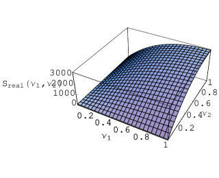
Figure 3: Interpolated estimate over the unit square of the real qubit-qutrit separability function $S_{real}(\nu_{1},\nu_{2})$, based on 785,000 randomly generated $6\times 6$ real density matrices

An immediate conjecture, suggested by our various earlier qubit-qutrit results (sec. III and (60)) is that this (naively, bivariate) function is actually univariate in nature, and satisfies the proportionality relation (cf. (93))

$$\mathcal{S}_{real}(\nu_{1},\nu_{2})=\mathcal{S}_{real}(\eta)\propto I_{\eta}(\eta,\frac{1}{2},2)=\frac{1}{2}(3-\eta)\sqrt{\eta}.$$ (97)

Here $\eta=\nu_{1}\nu_{2}=\frac{\rho_{11}\rho_{66}}{\rho_{33}\rho_{44}}$, being independent of $\rho_{22}$ and $\rho_{55}$ (given the definitions of $\nu_{1}$ and $\nu_{2}$ in eq. (44) above). (If we had chosen to compute the partial transpose of $\rho$ by transposing in place its nine $2\times 2$ blocks, rather than its four $3\times 3$ blocks, then presumably the same essential phenomenon would have occurred, but with different sets of indices on the $\nu$’s.) But, in fact, analyses we have conducted indicate that it is the (even simpler) univariate function satisfying the relation

$$\mathcal{S}_{real}(\nu_{1},\nu_{2})=\mathcal{S}_{real}(\eta)\propto\sqrt{\eta},$$ (98)

that fits the sample estimate of the separability function displayed in Fig. 3 extremely well.

To substantiate this last point, in Fig. 4, we show a plot of a least-squares fit of the normalized function shown in Fig. 3 to the function $\eta^{x}$, which for $x=\frac{1}{2}$ is identical to (98).

Figure 4: Least-squares fit of the normalized sample estimate of the real qubit-qutrit separability function displayed in Fig. 3 vs. $\eta^{x}=(\nu_{1}\nu_{2})^{x}$. The minimum of the curve is in the immediate vicinity of $x=\frac{1}{2}$, at which point the measure of goodness-of-fit is 0.00690362.

We see that the best fit does, in fact, suggest that $x=\frac{1}{2}$ is the appropriate choice (at least, within this one-parameter family of functions). (For the least-squares fit of (98) to our sample estimate, we obtain 0.00690362, while we obtain considerably more, that is 0.0184813, for the [inferior] fit of (97).) The product of the normalized function (98) with the corresponding jacobian is integrable in the real qubit-qutrit case (giving the result $\frac{131\pi}{1110124175582822400}\approx 3.70723\cdot 10^{-16}$).

If we adopt the ansatz (98) and employ the estimated value of the scaling constant for this function from Fig. 3, which is on the order of 3095.97, and additionally presume that the real qubit-qutrit HS separability probability (in line with our complex counterpart conjecture [immediately below] of $\frac{32}{1199}$—and qubit-qubit proposals of $\frac{8}{33}$ and $\frac{8}{17}$) is of the form $\frac{32}{k}$, where $k$ is some natural number, then our best estimate of this probability is $\frac{32}{213}\approx 0.150235$, and of the scaling constant $\frac{78848\pi^{8}}{139515\sqrt{3}}\approx 3096.05$. (We do not have highly extensive numerical estimates [only the more limited one pursued here] —as we did in the complex qubit-qutrit case Slater (2005b)—against which to gauge this prediction, but our fits here are strongly supportive of these assertions. For example, our sample estimate of the separability probability can be expressed as $\frac{32}{213.005}$.)

X.2 Complex Qubit-Qutrit Case

Based on our previous numerically-intensive study —using $10^{9}$ sample points —- we have an (implicitly-given) estimate (Slater, 2005b, between eqs. (38) and (39)) for the complex HS separability probability of 0.0266891. A very well-fitting candidate for the corresponding exact probability is $\frac{32}{1199}\approx 0.0266889$. (The associated separable volume would, then, be $\frac{\pi^{15}}{56980588975590080071885989375000\sqrt{6}}\approx 2.05327\cdot 10^{-25}$.) Aside from the striking goodness-of-fit, we see that the numerator of the probability is equal to $32=2^{n-1},n=6$, while in the qubit-qubit case, the numerator is $8=2^{n-1},n=4$. Also, the denominator $1199=109\cdot 11$, while $33=3\cdot 11$.

In line with the Dyson-indices pattern observed earlier, we investigated the possibility that the separability function in the complex qubit-qutrit case might be simply proportional to $\eta=\nu_{1}\nu_{2}$, that is, the square of its putative real counterpart, $\sqrt{\eta}$. The integral of the product of $\eta$ with the associated jacobian yields $\frac{829}{5045434342262725360252343040000}\approx 1.64307\cdot 10^{-28}$. With our proposal above (supported by the considerable numerical evidence of Slater (2007)) that the qubit-qutrit complex HS separability probability is $\frac{32}{1199}$, the scaling constant would be $\frac{537472\sqrt{\frac{2}{3}}\pi^{15}}{10063956375}\approx 1249.65$.

Figs. 5 and 6 are the complex qubit-qutrit counterparts of the (real qubit-qutrit) Figs. 3 and 4.

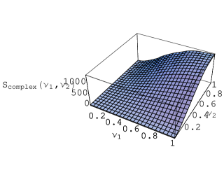
Figure 5: Interpolated estimate over the unit square of the complex qubit-qutrit separability function $S_{complex}(\nu_{1},\nu_{2})$, based on 880,000 randomly generated $6\times 6$ complex density matrices

Figure 6: Least-squares fit of the normalized sample estimate of the complex qubit-qutrit separability function displayed in Fig. 5 vs. $\eta^{x}=(\nu_{1}\nu_{2})^{x}$. We hypothesize that for a sufficiently large sample the minimum would lie at $x=1$.

Fig. 6 might be said to weakly support the proposal that the separability function is proportional to $\eta$. (The numerics here are perhaps yet insufficient for our purposes. In addition to only so far having sampled a relatively small number of complex $6\times 6$ density matrices, the sample points are now 30-dimensional in nature. For alacrity, we had simply used Monte Carlo methods, and not the [better-behaved/”lower-discrepancy”] quasi-Monte Carlo [Tezuka-Faure] methods employed in our earlier studies, in particular, in Slater (2005b, 2007). In light of the not very convincing nature of Fig. 6, it might be advisable to revert to the Tezuka-Faure scheme, although most of the unit hypercube points generated would, then, be simply discarded as not meeting the criteria a density matrix must fulfill. The most desirable/efficient sampling scheme, it seems, if it can be effectively implemented, would be the one associated with correlation matrices Joe (2006); Kurowicka and Cooke (2003, 2006a, 2006b), in which none of the generated points would have to be discarded.

XI Concluding Remarks

In a recent comprehensive review, it was stated that while quantum entanglement is “usually fragile to environment, it is robust against conceptual and mathematical tools, the task of which is to decipher its rich structure” (Horodecki et al., , abstract). We have attempted to make some progress in this regard here, but considerable impediments clearly still remain to putting the chief conjectures of this paper on a fully rigorous basis (or disproving them by establishing alternative results), and in proceeding onward to higher-dimensional cases. (In particular, we have not yet developed a theory to predict the scaling constants—$\frac{256\pi^{6}}{639}$ and $\frac{20\pi^{4}}{17}$ in the full complex and real two-qubit cases, and $\frac{537472\sqrt{\frac{2}{3}}\pi^{15}}{10063956375}$ and $\frac{78848\pi^{8}}{139515\sqrt{3}}$ in the full complex and real qubit-qutrit cases—for the hypothesized separability functions.) It would seem that applications and/or extensions of random matrix theory and, possibly, mathematical induction will be important—as they were in determining the total (separable and nonseparable) Hilbert-Schmidt volumes Życzkowski and Sommers (2003) (Bengtsson and Życzkowski, 2006, sec. 14.3) Andai (2006).

Let us, still, further suggest that the analytical framework and results, both theoretical and numerical, presented above may lead to the development of associated formal propositions, much in the way that the numerically-obtained (two-fold) separability-probability ratios reported in Slater (2005b) led Szarek, Bengtsson and Życskowski to establish that the set of separable (and, more generally, positive-partial-transpose) states is a convex body of constant height Szarek et al. (2006).

In Slater (a), we have further applied the “separability function” concept to the determination of the Bures (minimal monotone) metric volume of certain low-dimensional (real, complex and quaternionic) two-qubit states. Interestingly, we find that although the Dyson-index pattern is not now fully adhered too, it does come remarkably close to holding. Also, numerical research that we hope to shortly report, strongly indicates that in the full two-qubit quaternionic 27-dimensional Hilbert-Schmidt separable volume case, the Dyson-index pattern ($\beta=1,2,4$) we have observed above in the two-qubit 9-dimensional real and 15-dimensional complex cases (FIg. 2) is strictly maintained.