Shear-strain-induced Spatially Varying Super-lattice Structures on Graphite studied by STM

Abstract

We report on the Scanning Tunneling Microscope (STM) observation of linear fringes together with spatially varying super-lattice structures on (0001) graphite (HOPG) surface. The structure, present in a region of a layer bounded by two straight carbon fibers, varies from a hexagonal lattice of 6nm periodicity to nearly a square lattice of 13nm periodicity. It then changes into a one-dimensional (1-D) fringe-like pattern before relaxing into a pattern-free region. We attribute this surface structure to a shear strain giving rise to a spatially varying rotation of the affected graphite layer relative to the bulk substrate. We propose a simple method to understand these moiré patterns by looking at the fixed and rotated lattices in the Fourier transformed k-space. Using this approach we can reproduce the spatially varying 2-D lattice as well as the 1-D fringes by simulation. The 1-D fringes are found to result from a particular spatial dependence of the rotation angle.

I Introduction

Since the discovery of the scanning tunneling microscope (STM) by Binnig and Rohrer bin-roh , highly oriented pyrolytic graphite (HOPG) has been one of the most commonly used model surfaces for investigating and modeling of the STM imaging process. HOPG has a hexagonal structure with weakly coupled layers of graphene stacked in ABAB… sequence. Graphene is a semi-metal with zero density of states (DOS) at $E_{F}$ but a weak inter-layer interaction in graphite makes this DOS finite but small. This small DOS is quite sensitive to defects that influence the overlap of orbitals between layers kilic . This makes such defects easily visible by STM. Further, the weak inter-layer interaction makes such defects, like moiré patterns, possible near the surface of HOPG. A widespread study of this material has led to the discovery of several types of crystal imperfections native to the basal plane of HOPG. These include stacking faults, graphite strands and fibers, broken or flaked layers chang , super-lattices pong-rev ; kuwabara ; rong-kuiper ; xhie with periodicity of about ten nanometers or even larger, and the buckling of the top layer pong-buckling .

Broadly speaking, super-lattice structures in HOPG can occur due to three reasons. First type appears in graphite-intercalated compounds anselmetti with fixed period super-lattices like, $\sqrt{3}\!\times\!\sqrt{3}$ or 2$\times$2. Second type is the electron density oscillations (like Friedal oscillations) near point defects with a periodicity $\sqrt{3}$ times that of graphite mizes ; ruffieux . These oscillations decay rapidly as one moves away from the defect. The third one involves disorientation of one or more of the graphite layers near the surface kuwabara ; rong-kuiper ; xhie . This type of super-lattice structure is commonly known as moiré pattern and it arises as an interference pattern of two identical but slightly rotated periodic lattices. As first suggested by Kuwabara et. al. kuwabara , this rotation by a small angle $\theta$ gives rise to a super-lattice of the same symmetry but with much larger lattice constant given by, $D=d/(2\sin(\theta/2))$, with $d$ as the lattice constant of the original lattice. This super-lattice is rotated with respect to the original lattice by an angle $\phi=30^{\circ}-\theta/2$.

In this paper we present STM study of a spatially varying 2-D super-lattice pattern and 1-D fringes observed on HOPG (0001) surface near some defects. Such 2-D patterns have been reported earlier by several groups and are widely believed to be due to the moiré interference pong-rev ; kuwabara ; rong-kuiper ; xhie . Spatially varying periodicity patterns have also been reported before and have been attributed to a shear strain bernhardt or quantum confinement in a linear potential harigaya . The pattern observed here seems to be a result of an in-plane shear strain causing a spatially varying moiré rotation of a top layer. However, this is the first observation of linear fringes connected with a moiré pattern. We also discuss how these fringes can arise from a shear strain using a simple theory similar to the one proposed by Amidror and Hersch amidror1 ; amidror2 for moiré patterns in optics. This approach gives us a better analytical insight into the large scale structure of such patterns. An earlier model on moiré patterns in graphite is purely computational, based on the variation in local density of atoms pong-theory . In our model, the moiré patterns are examined in Fourier transformed k-space to quantify the variation in local stacking for a fixed as well as a spatially varying moiré rotation angle. Using this idea we can understand and simulate the above observed pattern and, in particular, the 1-D fringes.

II Experimental Details

Experiments were done with a home built STM similar to the one described elsewhere gupta-ng . This STM uses a commercial electronics and software rhk . The data reported here were taken in ambient conditions. HOPG was fixed on the sample holder with a conducting epoxy and the sample was freshly cleaved using an adhesive tape before mounting it on the STM. Fresh cut Pt_0.8Ir_0.2 wire of 0.25 mm diameter was used as the STM tip. The images have been obtained in constant current (feedback on) mode. The images shown here are filtered to remove steps and spikes, however, for quantitative analysis we have used the unfiltered data.

III Results

III.1 Spatially varying lattice and 1-D fringes

    

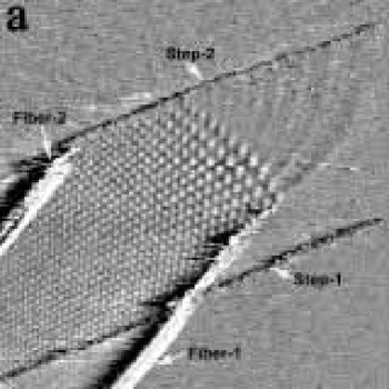
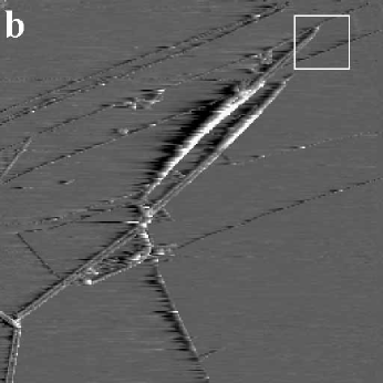
Figure 1: a. A STM image (0.32$\times$0.32 $\mu m^{2}$ at 0.5V and 0.2nA) showing a spatially varying super-lattice structure confined between fiber-1 and fiber-2 on the layer defined by step-1 and step-2. Near the termination of superstructure a 1-D fringe pattern appears. b. A later STM image (2.16$\times$2.16 $\mu m^{2}$ at 0.8V and 0.2nA) showing a larger portion of fiber-1 and fiber-2. The area of left image marked by the white square.

Fig.1a shows a topographic image of (0001) basal plane of HOPG with the super-lattice structure together with two steps and two carbon fibers. We mark these as fiber-1 & 2 and step-1 & 2. The step-1 is a double layer step with a height of 0.7$\pm$0.1nm while the step-2 is a single layer step. These step heights have been found from the images taken away from the super-lattice pattern area. These two steps divide the area into three terraces with the middle one having a super-lattice pattern confined between the two fibers as seen in the same figure.

Carbon fibers have been observed earlier by various groups on the graphite surface pong-rev . These, we believe, are long and thin ribbons or rolls of graphite created, presumably, during the cleaving process. The exact vertical location of the fibers relative to various visible layers is not so clear in this image. However, since the fibers are strictly limiting the pattern on the mono-layer terrace defined by step-1 and step-2, we believe that these fibers are in contact with this affected layer. They may be either below or above this particular layer. If a layer is above the fiber it would go over the fiber with some buckling. Such buckling cannot be ruled out by stress considerations as the fibers are quite wide ($\geq$10nm) and not so high ($\leq$1nm).

A relatively larger area image including the patterned region is shown in Fig.1b. This image was taken later when the fiber-1 was fully relaxed as discussed in detail later. The region of the left image is marked by a square in the right one. The other ends of the two fibers are also visible in Fig.1b. Here we see that the fiber-2 looks brighter above the step-1 and the fiber-1 has similar behavior but this is seen in the Fig.1a. Here, both the fibers look less bright when they emerge from the covered layer(s) near the center of the image in Fig.1b.

As shown in Fig.1a the super-lattice contains two regions namely a 2-D lattice extending till the end of fiber-1 and a 1-D wave-like pattern starting from the fiber-1 end. The 1-D fringes bend towards the step-2 and terminate at this step. The 2-D lattice continues beyond the fiber-2 end but terminates at step-2 in this image. The 1-D pattern contains the same number of maxima and minima as the terminating 2-D lattice. The 2-D lattice is not uniform as it evolves from a hexagonal lattice deep inside the fibers to nearly a square lattice with much larger periodicity. The super-lattice structure is also present over the step-1 (up to fiber-1) but with corrugation reduced by a factor of 2.3. Although this is not clearly visible in Fig.1 but we clearly see it on zooming into this area. The corrugation is also found to vary with periodicity as analyzed later.

III.2 Pattern variation with fiber-1 motion

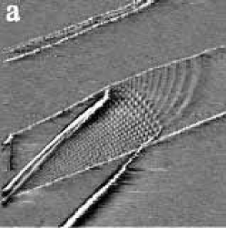
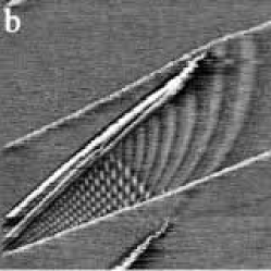
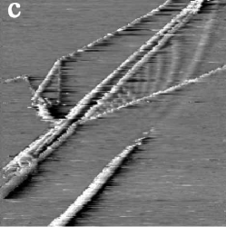
Figure 2: The topographic images of the super-lattice structure showing its evolution with the motion of fiber-1. a. 0.52$\times$0.52$\mu m^{2}$, b. 0.35$\times$0.35$\mu m^{2}$, c. 0.43$\times$0.43$\mu m^{2}$ taken at 0.5V and 0.2nA.

As we image this area repeatedly, fiber-1 becomes shorter in length as the whole fiber seems to recede. This may be due to some stress on the fiber. Several groups have reported various surface modifications in the STM experiments but the exact mechanism behind such modifications is not quite understood. We show three of the latter images in Fig.2 depicting the changing pattern with the fiber-1 withdrawal. The withdrawal of this fiber is not uniform with time as sometimes a significant length disappears in one scan and at other times it recedes gradually. Eventually the receding stopped and the length of the fiber stayed same over a couple of days. One remarkable observation is the pinning of the boundary between the 2-D super-lattice and the 1-D fringes to the fiber-1 end. With the receding of fiber-1, the 1-D fringes terminate on the fiber-2 as opposed to step-2 in earlier images. Moreover, the spatial extent and corrugation amplitude of 1-D fringes increases together with some modifications in the large scale structure of the 1-D pattern.

IV Analysis

Two close-up images of this pattern are shown in Fig.3 in two different regions of the structure at different orientation of the image window as compared to the previous ones. These images have been taken at an early stage when fiber-1 was extending the most. As apparent from the image shown in Fig.3a, the pattern deep inside the fibers (towards left) is a hexagonal lattice of fixed periodicity. As we move out, the periodicity increases with the pattern evolving to an oblique lattice and then to nearly a square lattice as seen in Fig.3b. Fourier transforms (FT) of these images as shown in the inset also illustrate this variation. In detail, the FT in Fig.3a shows six sharp spots while the FT in Fig.3b has these spots elongated.

 

   

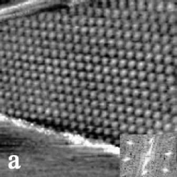
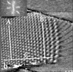
Figure 3: a. Super-lattice pattern image (120$\times$120nm² at 0.5V and 0.2nA) taken deep inside the fibers, and b. image (196$\times$196nm², 0.5V/0.2nA) taken near the boundary of the pattern. The insets show the respective Fourier transforms. c and d show the line scans along the lines A and B. e, f and g show the variation (along line C) in rms corrugation, periodicity, and rotation, respectively.

To analyze the periodicity variation carefully, line cuts were taken along various lines perpendicular to the line ‘C’ in Fig.3b. Two such representative lines are A and B along which the topographic height is plotted in Fig.3c and Fig.3d. These lines were carefully chosen to pass over the bright spots of the 2-D lattice. The periodicity along the lines perpendicular to C was found to be visibly constant but as one moves out along C this periodicity increases. The corrugation along the line C also varies. The RMS corrugation and periodicity as measured by line cuts perpendicular to C are plotted in Fig.3e and Fig.3f as a function of distance along the line C. The periodicity along such lines has been found from the average separation between peaks.

If we use the moiré rotation hypothesis, the rotation angle $\theta$ (between the top layer and the layers underneath) should also change spatially to get a varying lattice spacing D. Using $D=d/(2\sin(\theta/2))$ (d=0.246nm), we plot the variation of $\theta$ in Fig.3g. This varying $\theta$ implies that this rotated layer undergoes a shear as we move out of the fibers. The portion of this layer that is well inside the fibers has a constant rotation and the portion far outside the fibers is free of any moiré pattern and thus $\theta$ is zero. The intermediate region is strained with a changing $\theta$ and periodicity. As estimated from the periodicity, the angle $\theta$ changes from $2.3^{\circ}$ to $1.3^{\circ}$. The 1-D fringe pattern which has a close correlation with the 2-D moiré pattern prompts us towards a common origin for the two patterns. We believe that $\theta$’s particular spatial dependence is responsible for the 1-D fringes as discussed later.

A second order polynomial fit (as shown in Fig.3g) for this $\theta$ variation gives an expression,

$$\theta=A_{0}-A_{1}x-A_{2}x^{2}$$ (1)

with $A_{0}=(2.11\pm 0.02)$degree, $A_{1}=(3.0\pm 0.6)\times 10^{-3}$degree/nm, $A_{2}=(2.4\pm 0.5)\times 10^{-5}$degree/nm². This is also the expression for local angular orientation for a cantilever with one end clamped and the other end loaded cantilever .

A possibility on how the stress arises in the graphite layer is similar to the bending of a cantilever with certain loading conditions caused by the fibers. By the definition of strain, the maximum strain at a given $x$ would be $\frac{d}{2}\frac{d\theta}{dx}$. To estimate the maximum strain, the $\frac{d\theta}{dx}$ is maximum at the boundary of the 2-D super-lattice and 1-D fringes and it is found from the polynomial fit (Eq.1) to be (1.6$\pm$0.3)$\times$10^-4rad/nm. At this location the thickness (d) is 115nm. This point gives the largest stress, $\sigma_{max}$=1.1$\pm$0.2 GPa, using $Y$=121.9 GPa synder-prb for graphite. For comparison, the macroscopic indentation experiments indicate that stress on the order of $\approx$1 GPa damages the surface of graphite skinner . On the other hand, Snyder et. al. synder-prb have shown that the stress required to induce dislocation motion on basal plane of HOPG is of order 5-200 MPa.

V Understanding the linear fringes from spatially varying moiré rotation

Here we describe a simple model to understand and to simulate the large-scale structure of the spatially varying moiré patterns. For illustration, let us first consider a 1-D periodic lattice. If we superimpose two 1-D periodic patterns given by $\cos k_{1}x$ and $\cos k_{2}x$ ($\mid k_{1}-k_{2}\mid\ll k_{1},k_{2}$), we would see an interference (or beats-like) pattern with periodicity $2\pi/|k_{1}-k_{2}|$ in the superposed pattern (i.e., $\cos k_{1}x\cos k_{2}x$). In 2-D if we superimpose two hexagonal patterns of slightly different reciprocal lattice vectors ${\bf k_{i}}$ and ${\bf k_{i}^{\prime}}$ (i = 1-6), the resulting pattern in real space would come from the difference of the two sets of lattice vectors, i.e., (${\bf k_{i}^{\prime}-k_{j}}$). The longest period variations would arise from $\Delta{\bf k_{i}}={\bf k_{i}^{\prime}-k_{i}}$ (see Fig.4), which are actually responsible for the moirè patterns here. In 2-D, the pattern could arise due to differences in both the magnitude and direction of ${\bf k}$ and ${\bf k^{\prime}}$ amidror1 but in the present case only the direction mismatch is playing the major role.

    

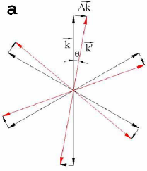
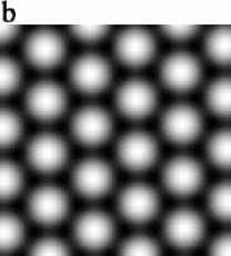
Figure 4: a The lattice vectors of the fixed ($\bf k$) and slightly rotated ($\bf k^{\prime}$) hexagonal lattices and their differences ($\bf\Delta k$). In this figure y-axis is pointing vertically up and x is pointing to the right. b Moiré interference pattern calculated using Eq.2 with a $\theta$=2.5^∘. The size of the image is 25$\times$25nm².

$\Delta{\bf k_{i}}$ as seen from Fig.4, has a magnitude of $2k\sin(\theta/2)$ and the smallest angle it makes with one of the ${\bf k_{i}}$’s is 30${}^{\circ}\!-\theta$/2. This is consistent with the aforementioned periodicity and angle of the moiré super-lattice. Now the moiré interference pattern in real space is easily produced by inverse Fourier transformation (IFT) of these six ${\Delta{\bf k_{i}}}$ vectors. This IFT gives a pattern described by,

$$I(x,y)=I_{0}\,+I_{1}[\cos(f{{}_{1}})+\cos(f{{}_{2}})+\cos(f{{}_{3}})],$$ (2)

where $I_{0}$ and $I_{1}$ are two constants and

$$f{{}_{n}}=2k\sin(\theta/2)\{-y\sin((n-1)\pi/3\!+\!\theta/2)\!+\!x\cos((n-1)\pi/3\!+\!\theta/2)\}].$$ (3)

Here n=1, 2 or 3 and $k=4\pi/\sqrt{3}d$ with $d$ (=0.246nm) as the real space ab-plane lattice parameter of graphite. Each cosine term in Eq.2 gives rise to a 1-D periodic pattern with bright and dark fringes along parallel straight lines (for constant $\theta$). The bright fringes of $\cos f_{n}$ are described by the contours $f_{n}(x,y)=2N\pi$, with N as an integer. For a constant $\theta$, the fringes due to the three cosine terms make an angle $\pi/3$ with each other and the sum of these three cosines leads to a 2-D triangular lattice pattern. One such pattern is shown in Fig.4b for $\theta=2.5^{\circ}$, $I_{0}$=0, and $I_{1}$=1. In this model, the $I(x,y)$ only quantifies the local stacking pattern. The $I(x,y)$ has a variation between +3 and -3 (taking $I_{0}=0$ and $I_{1}=1$) with a value of +3 signifying an AA stacking and -3 signifying an AB stacking. An intermediate value represents a slip with the degree of slip quantified by the magnitude of $I(x,y)$. The DOS at the surface is a result of top three layers and so the DOS at BAB and BAC could be actually different while our model does not differentiate between these two stacking sequences rong-kuiper ; xhie .

This model can also be used for the geometrically transformed lattices amidror2 , where the rotation angle is spatially varying. This way we can model the spatially varying moiré patterns and understand their large scale structure. In particular, we can find an analytical condition on the spatial variation of the rotation angle that gives rise to the 1-D fringes as following. For spatially varying $\theta$, the 1-D fringes due to each $\cos f_{n}$ will have a spatially varying periodicity and, in general, these fringes may not be straight and parallel to each other. These fringes will be locally perpendicular to $\nabla f_{n}$ and their local periodicity can be quantified by $2\pi/|\nabla f_{n}|$. These $f_{n}$’s (see Eq.3) satisfy the condition,

$$f_{1}=f_{2}-f_{3}.$$ (4)

For $I(x,y)$ to have a 1-D pattern, the fringes due to the contributing cosine terms must be locally parallel to each other or, in other words, each $f_{n}$ should have the same constant value contours. In particular, and as it turns out to be the case for the observed 1-D fringes, if the $\theta$ variation is such that $f_{1}=C$ (a constant) then using Eq.4, $f_{2}=C+f_{3}$. For such $\theta$ variations $\cos f_{1}$ gives no fringes while the fringes due to $\cos f_{2}$ and $\cos f_{3}$ are locally parallel with the same local wavelength. Thus $I(x,y)$ would have only 1-D fringes. Similar argument would also hold for $f_{2}$=constant or $f_{3}$=constant, which is obvious from symmetry considerations. The expression for $f_{1}$ (Eq.3) can be simplified to,

$$f_{1}=kx\sin\theta+ky(\cos\theta-1),$$ (5)

and so for $f_{1}(x,y)=C$ we find,

$$\theta(x,y)=sin^{-1}\left[\frac{(C/k)+y}{\sqrt{x^{2}+y^{2}}}\right]-tan^{-1}\left(\frac{y}{x}\right).$$ (6)

In small $\theta$ approximation we can neglect the ($\cos\theta-1$) term in comparison to $\sin\theta$ term in Eq.5 and this gives $\theta(x,y)=C/kx$. Here, one has to be careful in choosing the origin while using this form of $\theta(x,y)$. The same origin has to be used in calculating the $I(x,y)$ to ensure 1-D fringes. In fact this choice of origin gives one more parameter in choosing $\theta(x,y)$.

A simulated pattern using above ideas is shown in Fig.5b together with the observed pattern in Fig.5a. Here, we have used two different spatial forms of $\theta$ in different x intervals. We have used $\theta(x,y)$ as found in Eq.1 for 2-D region, where $\theta$ changes from 2^∘ to 1.29^∘. We use the small $\theta$ approximation for 1-D fringes, i.e., $\theta(x,y)=C/k(x+a)$ for $\theta$ between 1.29^∘ and 0.76^∘. The constants $C/k$ and $a$ are found to be 3.067 rad-nm and 4.399 nm, respectively, by ensuring the continuity of $\theta$ and $d\theta/dx$ at x=132.3 nm. This is necessary to keep the stress finite and continuous everywhere. For 1-D fringes the required $\theta(x,y)$ is of the form of $C/kx$, so in Fig.5, we have actually shown images of $I(x+a,y)$ with $a=4.399$ nm. A plot of the used $\theta$ variation as a function of $x$ is shown in Fig.5c. Since the 2-D to 1-D pattern boundary is pinned to the fiber-1 end we believe that there is a sudden change in spatial dependence of stress across this $x$ causing a change in $\theta$ behavior that in turn is responsible for the boundary. Fig.5 also shows the three $\cos f_{n}$ maps, where one can see clearly how the pattern arises in the two regions in terms of the three cosines as argued before. In the 1-D fringe region, we see that $\cos f_{1}$ gives no fringes while $\cos f_{2}$ and $\cos f_{3}$ have fringes that are locally parallel to each other. In the 2-D pattern region the fringes due to the three cosines are not parallel.

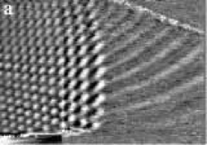
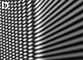
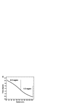
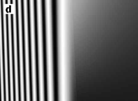
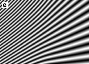
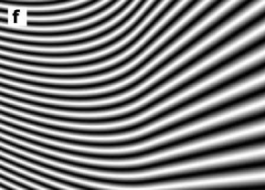
Figure 5: a. STM image of the super-lattice pattern of varying periodicity and linear fringes (196$\times$139nm² at 0.5V and 0.2nA). The 2-D pattern is present up to 100 nm and beyond this it changes into linear fringes b. Simulated image (see text) of size 198$\times$141nm² with the $\theta$ variation shown in c. d, e, f show the three cosine components, i.e., $\cos f_{1}$, $\cos f_{2}$ and $\cos f_{3}$, respectively, of the image in b. (In figures b, d, e and f y-axis is pointing at angle 3^∘ to vertically up and x-axis is perpendicular to y and towards the right.

So far we discussed a particular condition on $\theta$ that gives 1-D fringes. Now we find a more general condition on $\theta$ for getting 1-D fringes and we also argue here that above used spatial dependence of $\theta$ for 1-D fringes is the only possibility (in small $\theta$ approximation) for the observed fringes. The existence of 1-D fringes requires that all the constant value contours of $f_{1}$, $f_{2}$, and $f_{3}$ are identical. This is possible if $f_{1}=\phi(f_{3})$ and, using Eq.4, $f_{2}=f_{3}+\phi(f_{3})$, where $\phi$ is a scalar function. If we assume $\phi$ to be a linear function, i.e., $\phi(x)=\alpha(x+C_{1})$ then $f_{1}-\alpha f_{3}$=$\alpha C_{1}$. This, using Eq.3, gives the same solution for $\theta(x,y)$ as Eq.6 except for $x$, $y$, and $C$ replaced by $x^{\prime}=x(\alpha^{-1}+1/2)-y(\sqrt{3}/2)$, $y^{\prime}=y(\alpha^{-1}+1/2)+x(\sqrt{3}/2)$ and $C_{1}$, respectively. In small $\theta$ approximation, this gives $\theta(x,y)=C_{1}/kx^{\prime}$. Therefore, any function of the form $\theta(x,y)\propto 1/(x+\gamma y)$ would give rise to linear fringes for arbitrary $\gamma$ (=$\sqrt{3}\alpha/(\alpha+2)$). The form of $\theta$ used in producing the linear fringes in Fig.5 is a special case with $\alpha$=0 and $C_{1}\rightarrow\infty$ with $\alpha C_{1}$=C. From Fig.5a we see that the observed 1-D fringes connect smoothly to the rows of bright spots coming from $\cos f_{2}$ and $\cos f_{3}$ while the rows of bright spots due to $\cos f_{1}$ terminate before the 1-D fringes. This means that $\cos f_{1}$ is not contributing to the observed 1-D fringes and $\cos f_{1}$ has to be constant in this region. So $\theta=C/kx$ is the only possibility for the observed fringes in small $\theta$ approximation.

VI Discussion

Our simulation nicely captures most of the details of the observed pattern except for the curvature of the 1-D fringes. For the curvature in 1-D fringes, we find that any modification in spatial dependence of $\theta$ from $C/kx$ affects the 1-D nature more seriously than producing the curvature. Incidently, using the exact form of $\theta$ as in Eq.6 as opposed to its approximate form of $C/kx$ does not give the curvature either. Here, we believe that our approach of varying only the directions of ${\bf k^{\prime}}$s and not their magnitude is a bit oversimplified though it captures the general structure of both the 1-D and 2-D patterns. However, to get both the direction and magnitude of ${\bf k^{\prime}}$s requires a detailed understanding of the strain field in the affected region. This is not possible from the STM images alone as we have to know the stresses on the boundaries to solve the complete boundary value problem using elasticity theory.

As pointed out earlier, we should be cautious in using this model as this does not describe the quantitative contrast of an STM image. For instance, this model cannot explain the variation in corrugation amplitude of the 2-D super-lattice with its periodicity as seen from Fig.3e. The STM contrast here actually represents a DOS variation as our local tunneling spectra show that the bright regions are more metallic than the dark ones consistent with earlier work by Kuwabara et. al. kuwabara . As of now no calculations on electronic DOS on moiré patterns in graphite exist. A computational model was proposed by Hentschke et. al. hentschke and reviewed by Pong et. al. pong-theory , which is based on the variation in local density of atoms. In a sense our $I(x,y)$ also quantifies the local density of atoms but our model is more appropriate for the analytical understanding of the large scale structure of the spatially varying moiré patterns.

VII Conclusions

In conclusion, we have studied a spatially varying 2-D and a connected 1-D super-lattice structure on HOPG. This is the first observation of such 1-D fringes connected to a 2-D moiré lattice and we attribute this pattern to a spatially varying moiré rotation of a top graphite layer. The spatially varying rotation implies a shear strain in this layer. We have also described a simple model for understanding spatially varying moireé patterns. This model can successfully simulate the observed pattern by using a spatially varying rotation angle. The 1-D fringes are found to arise from a particular spatial dependence of the moireé rotation angle.

VIII Acknowledgements

The financial support from IITK under the ‘Initiation Grant’ scheme and from the MHRD of the Government of India is thankfully acknowledged. S K Choudhary acknowledge financial support from the University Grant Commission, Government of India.

References

- (1) :
- (2) G. Binnig, H. Rohrer, Ch. Gerber, and E. Weibel 1982 Phys. Rev. Lett. 49 57 .
- (3) C. Kilic, H. Mehrez, and S. Ciraci 1998 Phys. Rev. B 58 7872.
- (4) H. Chang and A. J. Bard. 1991 Langmuir 7 1143 ; C. Clemmer and T. Beebe. 1991 Science 251 640 ; S. Snyder, T. Foecke, H. White and H. Gerberich. 1992 J. Mater. Res. 7 341.
- (5) W.-T. Pong and C. Durkan 2005 J. Phys. D: Appl. Phys. 38, R329 .
- (6) M. Kuwabara, D. R. Clarke, and D. A. Smith 1990 Appl. Phys. Lett. 56 2396.
- (7) Z. Y. Rong and P. Kuiper 1993 Phys. Rev. B 48, 17427.
- (8) J. Xhie, K. Sattler, M. Ge, N. Venkateswaran 1993 Phys. Rev. B 47, 15835.
- (9) W. T. Pong, J. Bendall and C. Durkan 2005 Jap. J. Appl. Phys. (Part 1) 44 (7B) 5443.
- (10) D. Anselmetti, V. Geiser, G. Overney, R. Wiesendanger, and H.-J. Guntherodt 1990 Phys. Rev. B 42 1848.
- (11) H. A. Mizes and J. S. Foster 1989 Science 244 559; J. Xhie, K. Sattler, U. Müller, N. Venkateswaran, and G. Raina 1991 Phys. Rev. B 43 8917.
- (12) P. Ruffieux, M. Melle-Franco, O. Groning, M. Bielmann, F. Zerbetto, and P. Groning 2005 Phys. Rev. B 71, 153403.
- (13) T. M. Bernhardt, B. Kaiser, and K. Rademann 1998 Surf. Sci. 408 86 .
- (14) K. Harigaya, Y. Kobayashi, K. Takai, J. Rvier, and T. Enoki 2002 J. Phys. C 14 L605.
- (15) I. Amidror and R. D. Hersch 1996 J. Opt. Soc. Am. A 13 974.
- (16) I. Amidror and R. D. Hersch 1998 J. Opt. Soc. Am. A 15 1100.
- (17) W.-T. Pong and C. Durkan 2005 Japan. J. Appl. Phys. (Part 1) 44 (7B) 5365.
- (18) A. K. Gupta and K. -W. Ng 2001 Rev. Sci. Instrum. 72 3552.
- (19) RHK Technoogy, Troy, MI, USA.
- (20) Simple elasticity theory for a cantilever gives, (for small ) with as the force acting at one end of the cantilever, as the vertical deflection at a given . , , , and are the Young’s modulus, length, thickness, and the width of the cantilever, respectively.
- (21) S. R. Snyder, W. W. Gerberich, H.S. White 1993 Phys. Rev. B 47 10823 .
- (22) J. Skinner, N. Gane and D. Tabor 1971 Nature. Phys. Sci. 232 195.
- (23) R. Hentschke, B. Schurmann, and J. Rabe 1992 J. Chem. Phys. 96 6213.