Constrained flow around a magnetic obstacle

Abstract

Many practical applications exploit an external local magnetic field – magnetic obstacle – as an essential part of their construction. Recently, Votyakov et al. (2007) have demonstrated that the flow of an electrically conducting fluid influenced by an external field can show several kinds of recirculation. The present paper reports a 3D numerical study whose some results are compared with an experiment about such a flow in a rectangular duct. First, we derive equations to compute analytically an external magnetic field and verify these equations by comparing with experimentally measured field intensity. Then, we study flow characteristics for different magnetic field configurations. The flow inside the magnetic gap is dependent mainly on the interaction parameter $N$, which represents the ratio of the Lorentz force to the inertial force. Depending on the constrainment factor $\kappa=M_{y}/L_{y}$, where $M_{y}$ and $L_{y}$ are half-widths of the external magnet and duct, the flow can show different stationary recirculation patterns: two magnetic vortices at small $\kappa$, a six-vortex ensemble at moderate $\kappa$, and no vortices at large $\kappa$. Recirculation appears when $N$ is higher than a critical value $N_{c,m}$. The driving force for the recirculation is the reverse electromotive force that arises to balance the reverse electrostatic field. The reversion of the electrostatic field is caused by a concurrence of internal and external vorticity correspondingly related to the internal and external slopes in the $M$-shaped velocity profile. The critical value of $N_{c,m}$ quickly grows as $\kappa$ increases. For the case of well developed recirculation, the numerical reverse velocity agrees well with that obtained in physical experiments. Two different magnetic systems induce the same electric field and stagnancy region provided these systems have the same power of recirculation given by the $N/N_{c,m}$ ratio. The 3D helical peculiarities of the vortices are elaborated, and an analogy is shown to exist between a helical motion inside the studied recirculation and a secondary motion in the process of the Ekman pumping. Finally, it is shown that a 2D model fails to properly produce stable two and six-vortex structures as found in the 3D system. Interestingly, these recirculation patterns appear only as time dependent and unstable transitional states before the Karman vortex street forms, when one suddenly applies a retarding local magnetic field on a constant flow.

1 Introduction

An electrically conducting fluid flow influenced by a local external magnetic field is of considerable fundamental and practical interest. Applied to the flow, a transverse homogeneous magnetic field creates a so-called magnetic obstacle, i.e. a region where the flow motion is retarded by the Lorentz force.

On the fundamental side, such a system possesses a rich variety of dynamical states. This can already be imagined from the fact that its behavior is characterized by two parameters, the Reynolds number $Re=u_{0}H/\nu$ and interaction parameter $N=\sigma HB_{0}^{2}/\rho u_{0}$, where $H$, $u_{0}$, $B_{0}$ are characteristic scale, velocity and magnetic field induction, and $\rho$, $\nu$, $\sigma$ are density, kinematic viscosity, and electric conductivity of the fluid, see e.g. Shercliff (1962); Roberts (1967); Moreau (1990); Davidson (2001). $Re$ represents the ratio of the inertial to viscous forces in the flow, and $N$ represents the ratio of the Lorentz forces to the inertial forces. In ordinary hydrodynamics, such as a flow around a solid obstacle, an increase of the inertial force, i.e. $Re$, renders a system to the nonlinear dynamics characterized by a vortex motion past the obstacle, see Fig. 1$a$. The additional flow parameter $N$ brings new nonlinear degrees of freedom into the problem as was elaborated recently by Votyakov et al. (2007), see Fig. 1$b$.

On the practical side, spatially localized magnetic fields play an essential role in a variety of industrial applications in metallurgy, e.g. Davidson (1999), including stirring of melts by a moving magnetic obstacle (called electromagnetic stirring, e.g. Kunstreich (2003)), removing undesired turbulent fluctuations during steel casting using steady magnetic obstacles (called electromagnetic brake, e.g. Takeuchi et al. (2003)) and non-contact flow measurement using a magnetic obstacle (called Lorentz force velocimetry, e.g. Thess et al. (2006)). For instance, it is important to understand whether the useful turbulence-damping effect of a magnetic brake is obliterated by excessive vorticity generation in the wake of the magnetic obstacle.

As is well known in the flow past a solid obstacle, there is a stagnancy region where one can observe a recirculation in the appropriate Reynolds number regime, so called attached vortices shown in Fig. 1$a$. If instead of the solid obstacle one places a magnetic obstacle, by means of a local external magnetic field, then there will appear electrical eddy currents $\bf{j}$ which induce the Lorentz force $\bf{F_{L}=j\times B}$. The largest retarding effect occurs where the transverse magnetic field ${\bf B}$ is a maximum. Therefore, past the magnetic obstacle there is also a stagnancy region where a kind of a reverse flow might be obtained. This analogy between a solid and magnetic obstacle has been realized from the beginning of magnetohydrodynamics (MHD). In the earliest 2D numerical simulation, Gelfgat et al. (1978) have observed a kind of recirculation and marked an analogy with a solid body: ’the qualitative pattern of the streamlines in such a flow is similar to the situation which arises in the case of the flow around objects’. However, the specially designed physical experiments of Gelfgat & Olshanskii (1978) following upon this simulation failed to confirm their previous numerical results: ’special attempts which we made to detect zones with return flow were not successful. The negative flows which occur in certain numerical calculations are obviously due to inaccuracies in the calculation’. The authors of this quotation have been correct about the inaccuracies of the refereed 2D approach in the sense that this approach is not suitable to describe their experiments, nevertheless there have been still chances to reveal a kind of recirculation in the experiments. We shall discuss this item later in the Section 3.2.

For Western readers, the term ‘magnetic obstacle‘ has been revived in the work Cuevas et al. (2006a). (In the seventies of last century, one of the authors, Yu.K., used ‘magnetic obstacle‘ as a working term in Riga, MHD center of the former USSR). Cuevas et al. (2006a) have performed a 2D numerical study and described a Karman vortex street past the obstacle similar to those observed past a circular solid cylinder. We discuss a link between our 3D stationary and their 2D nonstationary results in Section 3.7.

Most recent results about the wake of a magnetic obstacle have been obtained by Votyakov et al. (2007). Their main result is presented in Fig. 1 where the qualitative structure of the wake of a magnetic obstacle is given in comparison with the wake of a physical obstacle. By means of 3D simulation and experiments, Votyakov et al. (2007) have found that the liquid metal flow shows three different regimes: (1) no vortices, when viscous force prevails at small Lorentz force, (2) one pair of inner magnetic vortices between the magnetic poles, when Lorentz force is high and inertia small, and (3) three pairs, namely, magnetic as in (2), connecting and attached vortices, when Lorentz and inertial forces are high. The latter six-vortex ensemble is shown in Fig. 1$b$.

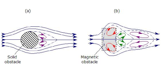
Figure 1: Structure of the wake of a solid ($a$) and magnetic obstacle ($b$). By forming the wake, the solid obstacle develops attached vortices, while the magnetic obstacle develops inner (first pair), connecting (second) and attached vortices (third pair).

An important factor for the flow influenced by an external magnetic field is the spanwise heterogeneity of the field. One can distinguish two extremal cases: (i) pointwise braking Lorentz force, and (ii) spanwise homogeneous braking Lorentz force. The latter case can be easily created, e.g. by external magnets long enough to overlap the duct, while the first case represents an idealization since it is impossible to have a pointwise external magnetic field. The first case is well studied in a 2D stratified flow, e.g. Voropayev & Afanasyev (1994); it is shown that a dipolar vorticity is generated in the vicinity of the origin of the point braking force. Applied to MHD flows similar results were obtained with a 2D numerical simulation of a creeping flow both in Gelfgat et al. (1978) and recently by Cuevas et al. (2006b). The vortex dipole observed in those works is of the same nature as the magnetic vortices that we will discuss in the present paper. The second case, spanwise homogeneous magnetic fields, is of traditional MHD interests and well understood. In particular, $M$-shaped profile is developed under streamwise magnetic field gradient, Shercliff (1962). It was studied extensively in experiments (Kit et al. (1970), Tananaev (1979)) and by numerical simulation (Sterl (1990),Votyakov & Zienicke (2007)). The most recent numerical paper (Votyakov & Zienicke (2007)) by comparing with experiment (Andreev et al. (2007)) has established that when turbulent pulsations are suppressed by an external magnetic field, it is the interaction parameter $N$ which governs the flow. It has been shown numerically that a spanwise homogeneous magnetic field is not able to reverse electric field inside the magnetic gap. As we shall prove below this is a necessary condition to induce recirculation between magnetic poles.

The goals of the present paper are the following: (1) report details not published in Votyakov et al. (2007) due to lack of space, (2) investigate thoroughly how a constrainment of MHD flow influences stationary vortex patterns, (3) explain the driving force for the recirculation, (4) find out what are the 3D peculiarities of the flow, and (5) clarify whether a 2D flow contains the observed stationary vortex patterns. It will be demonstrated that the decisive parameter for the constrained MHD flow is a power of the recirculation between magnetic poles given by the $N/N_{c,m}$ ratio, where $N_{c,m}$ is a critical value of the interaction parameter to induce magnetic vortices at the given magnetic field configuration. Moreover, several successful comparisons with available experimental data will be given for the intensity of the magnetic field, and for a maximal stationary reverse flow inside the magnetic obstacle. It will be explained that the magnetic vortices firstly appear due to the reverse electromotive force which is induced in order to balance the reverse electrostatic field inside the magnetic obstacle. Also, we will discuss a 3D versus 2D numerical approach and show that the found vortices have a 3D helical structure, while in a 2D model, at the given range of parameters, these vortices are not fixed by magnetic field and generate vortex shedding.

The subject of the present paper has a close connection to questions of stability of MHD flows, however, we have not included a full bifurcation analysis of new stationary flow patterns. The paper sheds light on the physical factors that determine the occurrence of stationary recirculation, i.e. the spanwise inhomogeneity of the magnetic field and the necessity of a three-dimensional geometry. We consider the bifurcation and stability analysis as a further step, which — from the practical point of view — also involves additional programming work on our code to allow for the computation of Jacobi matrices and their eigenvalues in a high dimensional dynamical system. Therefore, besides others, especially the following question will remain open: are the topological changes of the flow patterns, which we have observed in changing the system parameters, caused by changes of stability, i.e. bifurcations, or not (i.e. staying on the same solution branch but the solution only changes topology)? This and other open questions surely deserve further investigation for MHD channel flow in inhomogeneous magnetic field.

The structure of the present paper is as follows. Section 2 presents a sketch of the model, equations and a 3D numerical solver. As an essential part, it describes in Section 2.2 an analytical method to deal with magnetic field of arbitrary configuration. Section 3 presents the results of our numerical simulations: stationary flow patterns in the middle plane in Section 3.1, stability diagram in Section 3.3, mechanism for recirculation in Section 3.4, the 3D peculiarities of vortices in Section 3.6, as well as a relationship between 3D and 2D numerical methods in Section 3.7. Finally, the paper ends with a conclusion of the observations.

2 Problem Definition

2.1 Model, equations, numerical method

A schematic of the model is presented in Fig. 2: a conducting fluid flows in the rectangular duct of dimensions $\mbox{Length}\times\mbox{Width}\times\mbox{Height}=2L_{x}\times 2L_{y}\times 2H$ (half-length of the duct is shown); $x$-axis corresponds to the main direction of the flow. Top, bottom and side walls of the duct are no slip and electrically insulating. The magnets of horizontal dimensions $\mbox{Width}\times\mbox{Length}=2M_{y}\times 2M_{x}$ are assembled symmetrically on the top and bottom walls, where $2h$ is the distance between north and south poles. The center of the magnetic gap is the center of the coordinate system. The constrainment factor $\kappa=M_{y}/L_{y}$ defines the spanwise distribution of the magnetic field; $\kappa$ is the varied geometric parameter in the present simulations. Below, we will refer to the case of $\kappa=0.02$ as a magnetic blade, $\kappa=0.4$ as a middle magnet, and $\kappa=1.0$ as a broad magnet.

If nothing else is specified, throughout the paper the following geometric parameters have been taken: $L_{x}\!=\!25$,$\;L_{y}\!=\!5$, $\;H\!=\!1$, $\;h\!=\!1.5$, $\;M_{x}=1.5$, $\;0.02\!\leq\!\kappa\!\leq\!1$. Reynolds number, $Re$, and interaction parameter, $N$, are defined with half-height of the duct $H$, the mean flow rate $u_{0}$, and magnetic field intensity $B_{0}$ taken at the center of the magnetic gap, $x\!=\!y\!=\!z\!=\!0$.

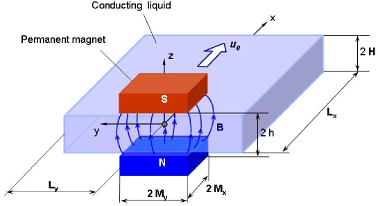
Figure 2: Sketch of the model. Through the paper it is used the constrainment factor $\kappa=M_{y}/Ly$, where $M_{y}$ and $L_{y}$ are half-width of the magnet and duct, correspondingly.

The governing equations for electrically conducting and incompressible fluid are derived from the Navier-Stokes equation coupled with the Maxwell equations for moving medium and Ohm’s law. We apply the quasi-static (induction-less) approximation where it is assumed that an induced magnetic field is infinitely small in comparison to the external magnetic field, see, e.g. Roberts (1967), and is therefore neglected when one calculates the Lorentz force, but it is not neglected when finding the electric current density j. The resulting equations in dimensionless form are:

$$\frac{{\partial\textbf{u}}}{{\partial t}}+(\textbf{u}\cdot\nabla)\textbf{u} = -\nabla p+\frac{1}{Re}\triangle\textbf{u}+N(\textbf{j}\times\textbf{B}),\;\;\;\nabla\cdot\textbf{u}=0,$$ (1)

j $$= -\nabla\phi+\textbf{u}\times\textbf{B},\;\;\;\;\nabla\cdot\textbf{j}=0,$$ (2)

where $\bf{u}$ denotes velocity field, $\bf{B}$ is an external magnetic field, $\bf{j}$ is electric current density, $p$ is pressure, $\phi$ is electric potential. The interaction parameter $N$ and Reynolds number $Re$, $N=Ha^{2}/Re$, are linked by means of the Hartmann number $Ha$: $Ha=HB_{0}(\sigma/\rho\nu)^{1/2}$. The Hartmann number determines the thickness of Hartmann boundary layers, $\delta/H\sim Ha^{-1}$ for the flow under constant magnetic field. For a given conducting fluid and geometry of the duct, one varies either the flow rate velocity $u_{0}$, i.e. $Re$, or the magnetic field intensity $B_{0}$, i.e. $Ha$. In both cases, $N$ changes.

At given external field $\bf{B}$, the unknowns of the partial differential equations (1 – 2) are the velocity vector field ${\bf u}(x,y,z)$, and two scalar fields: pressure $p(x,y,z)$ and electric potential $\phi(x,y,z)$. For no-slip and insulating walls, the boundary conditions are $u|_{\Gamma}=0$, $\partial\phi/\partial{\bf n}|_{\Gamma}=0$, where ${\bf n}$ is normal vector to a surface $\Gamma$. The outlet of the duct was treated as a force free (straight-out) border for the velocity. The electric potential at inlet and outlet boundaries was taken to be equal to zero because the inlet and outlet are sufficiently far from the region of magnetic field. The stationary laminar profile of an infinite rectangular duct known analytically in the form of a series expansion was used as the inlet velocity profile. Because we are interested in a stationary solution, the initial conditions play no role (except for the speed of convergence).

The 3D numerical solver has been described in details in Votyakov & Zienicke (2007). It was developed from a free hydrodynamic solver created originally in the research group of Prof. Dr. M. Griebel (Griebel et al. (1995)). The solver employs the Chorin-type projection algorithm and finite differences on an inhomogeneous staggered regular grid. Time integration is done by the explicit Adams-Bashforth method that has second order accuracy. Convective and diffusive terms are implemented by means of the VONOS (variable-order non-oscillatory scheme) scheme. The 3D Poisson equations for pressure and electric potential, arising at each time step, are solved by using the bi-conjugate gradient stabilized method (BiCGStab).

The computational domain, $|x|\!\leq\!L_{x}$, $\;|y|\!\leq\!L_{y}$, $\;|z|\!\leq\!H$, has been discretized by an inhomogeneous regular 3D grid described in detail in Votyakov & Zienicke (2007). To verify that the inlet and outlet boundaries have no influence on the presented results, we have carried out several simulations with double the number of grid points in the $x$-direction and found no differences. Moreover, we have also varied the inhomogeneous grid resolution both in $y$ and $z$-direction to be sure that Hartmann and sidewall layers are properly resolved.

2.2 Fast analytical method for a proper magnetic field

As is imposed by the electrodynamics, an external magnetic field must be divergence and curl-free. Although authors of previous works realized this fact, to define their fields they used simple mathematical functions which did not satisfy divergence and/or curl-free requirements, see, e.g. Sterl (1990), Alboussiere (2004). This fact might be explained by many reasons, e.g. either by the complexity of a real field or insignificance of effects appearing due to an inaccuracy of the field definition. Therefore we feel that there are insufficient correct and yet simple methods to define an external magnetic field of arbitrary configurations. To fill this gap we explain below a simple physical approach which can be easily extended and implemented into 3D numerical models.

We assume that a magnet is composed of perfectly aligned pointwise magnetic dipoles having the same magnetic moment. This assumption is well posed for modern manufactured permanent magnets, as follows from the final comparison between calculated and experimentally measured magnetic field. Take $z$ as a direction of the unit magnetic dipole ${\bf m}=(0,0,1)$, then, a partial magnetic field in point ${\bf r}=(x,y,z)$ from a dipole located in point ${\bf r^{\prime}}=(x^{\prime},y^{\prime},z^{\prime})$ can be presented as, see e.g. Jackson (1999):

$$\bf{B^{\prime}(r,r^{\prime})} = \nabla\times\left[{\bf m}\times\frac{{\bf R}}{R^{3}}\right]=\nabla\times\left[-{\bf m}\times\left(\nabla\frac{1}{R}\right)\right]$$ (3)

$$= \nabla\times\left[\nabla\times\left(\frac{{\bf m}}{R}\right)-\frac{1}{R}\nabla\times{\bf m}\right]=\nabla\left[\nabla\cdot\frac{{\bf m}}{R}\right]=\nabla\frac{\partial}{\partial z}\frac{1}{|{\bf r-r^{\prime}}|},$$

where ${\bf R}={\bf r-r^{\prime}}$ and $R=|{\bf r-r^{\prime}}|$. Here we used ${\bf R}/R^{3}=-\nabla(1/R)$ along with few vector identities and omitted the constant $\mu_{0}/(4\pi)$. Then, the total field from a magnet occupying a space $\Omega$ follows as:

$${\bf B(r)}\!=\!\int_{\Omega}{\bf B^{\prime}(r,r^{\prime})}d{\bf r^{\prime}}\!=\!\nabla\frac{\partial}{\partial z}\Phi({\bf r}),\;\;\Phi({\bf r})=\int_{\Omega}\frac{d{\bf r^{\prime}}}{|{\bf r-r^{\prime}}|}$$ (4)

The last integral can be computed analytically in some cases as we show below. For an arbitrary $\Omega$, the integration can be performed only numerically and then be once tabulated in a 3D array. This 3D array can be supplied into a numerical solver where a finite differentiation is applied to compute the external magnetic field. Another way is to differentiate analytically $1/|{\bf r-r^{\prime}}|$ and then calculate numerically three integrals for each magnetic field component.

When limits of the integration imposed by $\Omega$ are independent of each other, then the problem has an analytical solution by means of the indefinite integrals given in Appendix A.

As shown in Fig. 2, the magnetic dipoles are located in the region $\Omega=\{|x^{\prime}|\leq M_{x},|y^{\prime}|\leq M_{y},h\leq|z^{\prime}|\leq\infty\}$, where $2h$ is a distance between north and south magnetic poles. In the present paper, the condition $|z^{\prime}|\geq h$ is assumed because the magnets used in the experiments are assembled onto a soft-iron yoke that closes magnetic field lines, i.e. the dipoles are effectively located from $h$ up to infinity. By taking the corresponding derivatives of indefinite integrals given in Appendix A, and after a few algebraic calculations one obtains:

$$B_{x}(x,y,z) = \frac{1}{B_{0}}\sum_{k=\pm 1}\sum_{j=\pm 1}\sum_{i=\pm 1}(ijk)\,\mbox{arctanh}\left[\frac{y-jM_{y}}{r(i,j,k)}\right],$$ (5)

$$B_{y}(x,y,z) = \frac{1}{B_{0}}\sum_{k=\pm 1}\sum_{j=\pm 1}\sum_{i=\pm 1}(ijk)\,\mbox{arctanh}\left[\frac{x-iM_{x}}{r(i,j,k)}\right],$$ (6)

$$B_{z}(x,y,z) = -\frac{1}{B_{0}}\sum_{k=\pm 1}\sum_{j=\pm 1}\sum_{i=\pm 1}(ijk)\,\mbox{arctan}\left[\frac{(x-iM_{x})(y-jM_{y})}{(z-kh)r(i,j,k)}\right],$$ (7)

where $r(i,j,k)=[(x-iM_{x})^{2}+(y-jM_{y})^{2}+(z-kh)^{2}]^{1/2}$, and $B_{0}$ is selected in such a way to have $B_{z}(0,0,0)=1$. Three-fold summation with the sign-alternating factor $(ijk)$ reflects the fact that these equations are obtained by integrating according to Eq. (4).

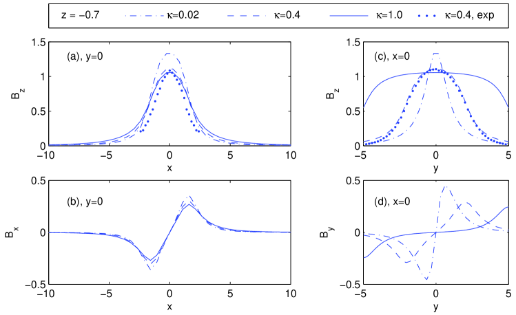
Figure 3: Comparison of computed (lines) and experimental (symbols) magnetic field intensities at different $\kappa=M_{y}/L_{y}$, $\kappa=0.02$ (dot-dashed), $0.4$ (dashed and symbols) and 1.0 (solid), $z=-0.7$: $B_{z}$ component along $x,\;y=0$, ($a$), $B_{x}$ component along $x,\;y=0$, ($b$), $B_{z}$ component along $y,\;x=0$, ($c$), $B_{y}$ component along $y,\;x=0$, ($d$).

Fig. 3 shows cuts of magnetic field intensities computed with equations (5-7) for different $\kappa$. Also, few experimental data (symbols) are presented for $\kappa=0.4$. There is a good agreement between experimental and analytical results. Moreover, one can see that the constrainment factor $\kappa$ affects mainly the spanwise distribution of magnetic field, whereas streamwise distribution changes only slightly. This is expected, because the length $M_{x}$ of the magnet is fixed, while the width $M_{y}=\kappa L_{y}$ is varied. It is necessary to note that even for the broad magnet ($\kappa=1.0$) there is still a decline of $B_{z}$ near side walls, Fig. 3($c$).

Contour lines of the $B_{z}$ component in the middle plane ($z=0$) at different $\kappa$ are also shown in Fig. 4($a-c$).

Thus, we have demonstrated a self-consistent analytic approach to define arbitrary magnetic field configurations. It guarantees divergence- and curl-free requirements of ${\bf B(r)}$ and has a link with a clear physical model.

3 Results and Discussion

3.1 Stationary flow patterns in the middle plane

In Section 3.1 we discuss characteristic stationary flow patterns which have been extracted from 3D numerical results. Three-dimensionality of the simulations is of importance to make these patterns stable, as we shall show later in Section 3.7.

3.1.1 Streamlines for different constrainment $\kappa$

In our opinion the most striking effect of spanwise heterogeneity of the external magnetic field is shown in Fig. 4, where flow streamlines in the middle plane, Fig. 4($d-f$), are shown at the same flow parameters, $N=36$ and $Re=196$. To get an impression about the magnetic field configurations, the corresponding $B_{z}$ contour lines are shown in Fig. 4($a-c$). Depending on the constrainment factor $\kappa$, one observes the following stationary flow patterns: a vortex dipole for the magnetic blade ($\kappa=0.02$), Fig. 4($a,d$); the stable six-vortex ensemble for the middle magnet ($\kappa=0.40$), Fig. 4($b,e$); and no vortex motion for the broad magnet ($\kappa=1.0$), Fig. 4($c,f$). The projection of the magnetic pole onto the middle plane is shown by the bold solid line.

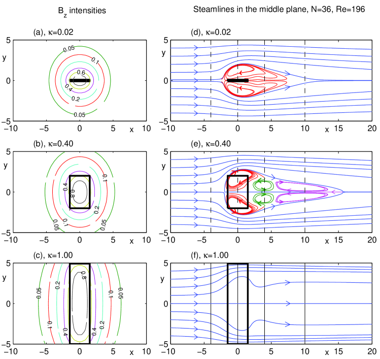
Figure 4: Contour lines of the transverse magnetic field component ($a$-$c$) and flow streamlines ($d-f$) in the middle plane ($z=0$) at $N=36$,$\;Re=196$ and $\kappa=0.02$ ($a,d$), 0.4($b,e$), and 1.0($c,f$). Magnetic pole is shown by bold lines. Dot-dashed($d$), dashed($e$) and solid($f$) vertical cuts denote the location of velocity profiles of Fig. 5.

Let us qualitatively explain these flow patterns. The case of the magnetic blade, Fig. 4($a,d$), might be roughly understood by considering the limiting case of a Lorentz force which is pointwise in the spanwise direction. (By its definition, ${\bf F_{L}=j\times B}$, the Lorentz force is a volume force, however, if the distribution of heterogeneous magnetic field $\bf B$ is very sharp in space, the Lorentz force distribution is also very sharp.) As is known, see e.g. Voropayev & Afanasyev (1994), such an instant retarding force generates vorticity which results in two counter-rotating vortices, a vortex dipole. Then, the induced vortices are advected and diffused downwards from the source of the force. In the case of MHD flow, these two vortices are fixed by a sidelong gradient of the magnetic field, so they stay on the place. We should note that the similar recirculation has been obtained numerically earlier by Gelfgat et al. (1978), and recently by Cuevas et al. (2006b) for a creeping flow.

The case of the middle magnet, Fig. 4($b,e$), is explained briefly in the recent work of Votyakov et al. (2007) by means of a mutual interaction of Lorentz and inertial forces. The first pair – inner magnetic vortices – is an inheritor of the vortex dipole as in Fig. 4($d$); the third pair – attached vortices – is of the same nature as a recirculation past a solid body, Fig. 1($a$), while the intermediate pair – connecting vortices – appear to make the coherent rotation of the magnetic and attached vortices possible, Fig. 1($b$),  4($e$). It is clear why attached (hence, connecting) vortices are not induced in the case of the magnetic blade: it has a well streamlined shape, so there is no stagnancy region. This is in full analogy with the flow around a solid body where an appearance of the stagnancy region is strongly influenced by extent of streamlining.

Finally, the case of the broad magnet, Fig. 4($c,f$) shows no recirculation at given parameters, because the flow pattern is influenced now mainly by streamwise inward and outward gradients of the magnetic field. As is known, see e.g. Shercliff (1962), Kit et al. (1970), Sterl (1990), the streamwise gradients and sidewalls of the duct are responsible all together for a $M$-shaped profile of a streamwise velocity in the spanwise direction. The $M$-shaped profile can also develop a stagnant region in the middle of the duct at high interaction parameter $N$, however, no recirculation has been discovered until now. Moreover, as we shall prove in Section 3.4, no recirculation is possible if an external magnetic field is perfectly spanwise uniform. The present case of the broad magnet shows a slight decline of $B_{z}$ moving towards sidewalls, see Fig. 3($c$, solid line). In Fig. 4($c$), however, this decline is not enough to develop magnetic vortices at the given interaction parameter $N=36$. We will see later that the critical interaction parameter $N_{c,m}$ which is needed to induce recirculation under the broad ($\kappa=1.0$) magnetic gap is more than one hundred.

3.1.2 Velocity profiles at different $\kappa$ and the same $N$ and $Re$.

Fig. 5 shows quantitative data about stream- and spanwise velocity along different spanwise cuts. Different line styles correspond to the different $\kappa$’s. Arrows in Fig. 5 show directions of a spanwise redistribution of the flow.

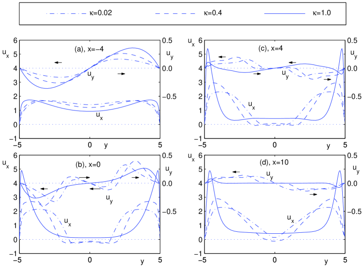
Figure 5: Streamwise ($u_{x}$, three lower curves, left $y$-axis) and spanwise ($u_{y}$, three upper curves, right $y$-axis) velocities along spanwise cuts shown in Fig. 4($d-f$). Middle plane, $z=0$, and $\;x=-4$($a$), $\;x=0$($b$), $\;x=4$($c$), $\;x=10$($d$). Constrainment factor $\kappa=0.02$ (dot-dashed), $\kappa=0.40$(dashed), and $\kappa=1.0$(solid lines), $N=36,\;Re=196$. Arrows show directions of spanwise redistribution of the flow.

The largest braking Lorentz force, ${\bf F_{L}=j\times B}$, is generated at the front of a magnetic obstacle where induced electric currents ${\bf j}$ are maximum and the magnetic field ${\bf B}$ is strong. This results in a deformation of the incoming flow on the obstacle already at $x\!=\!-4$, Fig. 5($a$). The deformation consists of forming an inhomogeneous $M$-shaped profile of streamwise velocity $u_{x}$ and an appearance of a spanwise flow, i.e. $u_{y}$, from the center to sidewalls, as shown by arrows in Fig. 5($a$).

Despite the order of magnitude difference in spanwise widths of magnets for $\kappa=0.02$ (dot-dashed) and $\kappa=0.4$ (dashed), their ranges of reverse velocity ($u_{x}\!\leq\!0$, Fig. 5($b$)) along the $y$-axis differ only by a factor one and half in the area of magnetic vortices. Positive streamwise velocities of the vortices are smoothly transformed into velocities of the external flow. Thus, for the wide range of $\kappa$, the spanwise diameter of a single magnetic vortex remains nearly constant provided the vortex is not influenced by a sidewall. This is a manifestation of the fact that a decisive role for the vortex is the width of the spanwise decline of a magnetic field rather than the width of the magnet.

By forming magnetic vortices, the $M$-shaped profile of streamwise velocity $u_{x}$ develops a negative value in the center, while the spanwise velocity $u_{y}$ changes its sign twice. There is a redistribution of the flow from a vortex inner side to the centerline ($y=0$), and from an external side of the vortex to the corresponding sidewall ($y=L_{y}$). On the contrary there are distinct zones past the magnetic vortices where a spanwise redistribution is absent ($u_{y}\!=\!0$), see $|y|\!\leq\!0.8$ for the magnetic blade ($\kappa=0.02$, dot-dashed) and $|y|\!\leq\!1.5$ for the middle magnet (dashed), Fig. 5($c$). Also, the zone of $u_{y}=0$ is observed behind attached vortices, $|y|\!\leq\!1$, Fig. 5($d$), $\kappa=0.4$.

Streamwise component of the velocity shows small changes with rising $x$, cf. $u_{x}$ in Fig. 5($b-d$), except for a single peculiarity. For the case of a broad magnet ($\kappa=1$, solid lines), one observes that as $x$ increases, the maximum of $u_{x}$ is shifted from sidewalls to the center due to diffusion of vorticity. In the same time, the $u_{y}$ component changes its sign in the region near sidewalls.

3.2 Centerline profiles

In this Section, taking as an example the middle magnet, $\kappa=0.4$, we show what forces are needed to induce vortices inside and past a magnetic obstacle. To reach this goal we shall analyze streamwise velocities along the centerline of the duct ($y=z=0$), i.e. centerline profiles.

The main difference between a magnetic obstacle and a solid body is the permeability of the obstacle depending on the retarding Lorentz force, ${\bf F_{L}=j\times B}$. This braking force is the largest in the center of the magnetic obstacle, where the magnetic field ${\bf B}$ reaches the highest intensity. The characteristic measure of the Lorentz force with respect to inertia is given by the interaction parameter $N$: higher the $N$, the stronger is ${\bf F_{L}}$ and less penetrable is the space under the magnets. Fig. 6($a$) is to illustrate this behavior: a dot-dashed line ($N=4$) shows that the streamwise velocity is suppressed by approaching the magnet, however the braking force for the given $N$ is not strong enough to reverse the flow. The reversion happens at higher $N$, see dashed ($N=9$) and solid ($N=16$) lines being negative inside the obstacle. The lowest velocity is marked in Fig. 6($a$) by $u_{\mbox{\scriptsize{x,min}}}$, it becomes zero at a critical value $N_{c,m}$, and at $N\geq N_{c,m}$ one observes a recirculation – two inner magnetic vortices as shown in Fig. 4($d,e$). As the name points out, these vortices belong completely to the MHD flow, and have nothing common with a hydrodynamical flow around a cylinder. Rather these vortices are similar to those appearing under the action of a point braking force, see e.g. Afanasyev (2006). The concrete mechanism leading to the magnetic vortices is presented in Section 3.4.

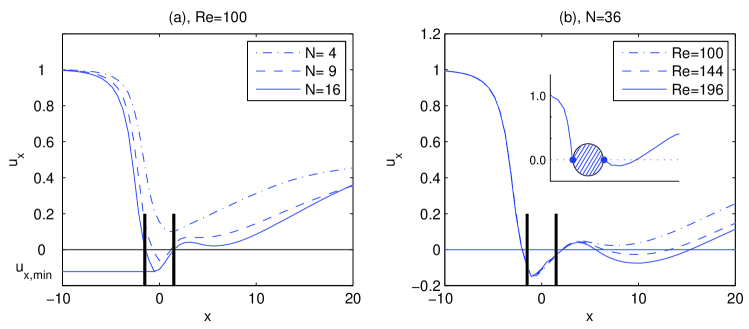
Figure 6: Streamwise velocity varied along the centerline $y=z=0$ for the middle magnet ($\kappa=0.4$): effect of $N$ at fixed $Re=100\;$ ($a$); and effect of $Re$ at fixed $N=36\;$ ($b$). For ($a$): $N=4$(dot-dashed), 9(dashed), and 16(solid lines); for ($b$): $Re=100$(dot-dashed), 144(dashed), and 196(solid lines). Vertical bold lines show borders of the magnetic gap, $M_{x}=1.5$. Inset in ($b$) is a centerline velocity profile for a flow around a circular cylinder with attached vortices. The streamwise velocity is normalized to the centerline velocity of unretarding flow.

Now, we consider the behavior of centerline curves at fixed $N$ and varying $Re$, Fig. 6($b$) and apply the analogy with ordinary hydrodynamics. Let us recall that the flow around a solid cylinder shows a stagnant region with two attached vortices when $Re$ is slightly higher than a critical value. The typical centerline for this case is shown by inset of Fig. 6($b$). The same situation can happen for the magnetic obstacle by increasing $Re$: the centerline curves past the magnetic gap become negative again as shown in Fig. 6($b$). In fact, the attached vortices are induced past the magnetic obstacle, see Fig. 4($e$, third pair of vortices) analogous to those past a real solid body.

Note, that the first minimum in a centerline profile is almost unperturbed when $Re$ increases at fixed $N$, Fig. 6($b$), and this is another strong evidence that the vortices inside and past the magnetic obstacle are of different physical origin. Since the interaction parameter is given as $N=Ha^{2}/Re$, the magnetic vortices are enhanced by decreasing the flow rate (i.e.  $Re$). On the contrary, as follows from Fig. 6($b$), the attached vortices manifest themselves by increasing the flow rate provided that the intensity of the magnetic field (i.e. $Ha$) as well as a spanwise magnetic field gradient have already enforced a reverse flow inside the magnetic obstacle. In other words, there is a qualitative distinction between magnetic and attached vortices: the former arise when Re decreases, and the latter arise when Re increases provided Ha is strong.

It is easy to see in Fig. 4($e$) that magnetic and attached vortices are co-rotating in the same direction determined by the main flow movement. The only difference is the driving torque: this is the Lorentz force for the magnetic vortices, and the inertial force for the attached vortices. Because the magnetohydrodynamic and attached vortices are co-rotated, such a motion must be accompanied by a counter-rotation which produces the intermediate pair of connecting vortices, see Fig. 4($e$, second pair of vortices). The connecting vortices correspond to a local maximum on centerline curves, Fig. 6($b$) behind the magnetic gap.

Thus, $N$ is responsible for the appearance of the magnetic vortices, while $Re$ is responsible for the appearance of the attached vortices. The connecting vortices are necessary for the coherent rotation of the magnetic and attached vortices.

Three decades ago Gelfgat et al. have attempted to reveal a kind of recirculation due to an external magnetic field by both 2D numerical simulation (Gelfgat et al. (1978)) and physical experiments (Gelfgat & Olshanskii (1978)). They saw a reverse flow numerically, and then designed a special experiment which did not confirm the recirculation. As follows from our results, the authors of the cited papers have not realized that they observed and discussed different phenomena in their numerical and experimental works. Their 2D numerical study neglected an inertial term, what corresponds to a creeping flow, and the observed reversion of the flow is just a sign of magnetic vortices. Recently, similar 2D numerical work of Cuevas et al. (2006b) showed the same effect in a creeping flow without side walls. Thus, the numerical work of Gelfgat precedes Cuevas et al. (2006b) by almost thirty years.

The experimental report of Gelfgat & Olshanskii (1978) contains a measured centerline profile (see Fig.7b in the cited work), which falls behind the magnet, but does not approach negative velocities. In the cited experiment, parameters are $N=7.5$ and $Re=3.73\times 10^{5}$, so the authors noticed that the observed falling velocity is due to inertial effects. Moreover, these experiments were performed for the turbulent flow because $Re$ is rather high. To obtain the desired recirculation, the authors needed to just decrease further the inertial force by using a lower flow rate. This would have resulted in a higher $N$ and, by exceeding some threshold, made impossible the turbulent pulsations. Then, the recirculation by the braking Lorentz force might have been revealed with the appearance of magnetic and attached vortices. Unfortunately, experiments with lower $Re$ have not been performed, probably because the proper analysis of centerline curves (see Fig.6) has been absent in those times.

3.3 Existence regions of stationary flow patterns in parameter space

A sign of the recirculation enforced by the Lorentz force is the negative value of $u_{\mbox{\scriptsize{x,min}}}$, see Fig. 6($a$). We have performed a series of 3D simulations for the different interaction parameters $N$ and constrainment factors $\kappa$. An example of the series for the middle magnet ($\kappa=0.4$) is shown in Fig.7($a$). It is accompanied by experimental data which were obtained by Oleg Andreev for the paper Votyakov et al. (2007) but not reported there due to lack of space. Note, that the interaction parameter $N=Ha^{2}/Re$ is changed in experiments and numerics differently: experimentally by varying the flow rate (i.e. $Re$) at fixed external magnets (experimental $Ha=140$), while numerically we kept $Re$ constant and changed $Ha$. This is because of (i) experimental difficulties to work with a low flow rate in the closed channel, and (ii) numerical problems arising due to boundary layers at high Hartmann numbers. Moreover, a transition to turbulent regime is another factor that obscures stationary effects in numerics at high $Re$.

As one can see in Fig. 7($a$), $u_{\mbox{\scriptsize{x,min}}}$ is positive at low $N$, and then falls monotonically to a constant level showing perfect agreement between experiments and numerics for $N>15$. This excellent agreement confirms that the flow under magnets depends solely on $N$ and magnetic field configuration rather than $Re$ or inlet profile, provided, the external magnetic field is strong enough to suppress inward turbulent fluctuations. The latter condition was satisfied in experiments by Andreev et al. (2007). Also, a similarity of the electric potential map at equal $N$ and different $Re$ has been recently confirmed by 3D simulations and comparison with experiments, see Votyakov & Zienicke (2007). The slight difference shown in Fig. 7($a$) at $N<15$ is explained by the fact that the variation for $N$ has been defined differently in experiments and numerics, as explained above.

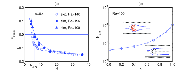
Figure 7: Plot ($a$): minimum of streamwise velocity on the centerlines curves (see Fig. 6$a$) depending on the interaction parameter $N=Ha^{2}/Re$ obtained in simulations (closed symbols) and in experiments (open circles) for $\kappa=0.4$ and $Ha=140$ (experiment), $Re=196$ (squares) and $Re=100$ (triangles). Plot ($b$): The critical interaction parameter $N_{c,m}$ depending on $\kappa$ for the appearance of magnetic vortices, 3d simulation, $Re=100$.

Dependence of $u_{\mbox{\scriptsize{x,min}}}$ on $N$ becomes negative at a critical value $N_{c,m}$. This value depends on the constrainment factor $\kappa$. A series of 3D simulations has been carried out for the range $0.02\leq\kappa\leq 1$ in the vicinity of $u_{\mbox{\scriptsize{x,min}}}(N)\approx 0$ and the results are given in Fig. 7($b$) which shows the separation line between regions for stable flow without and with magnetic vortices. During this series of 3D simulations we did never find a hint that both flow patterns — the one with and the one without magnetic vortices — coexist for the same pair of parameters, i.e. both solutions are stable, but have different basins of attraction. However, we have checked different initial conditions only for some parameter combinations and did not carry out a systematic search with different initial conditions. Therefore, we can not conclude that the case of coexistence of two solutions is not possible.

From the separation line of Fig. 7($b$), as we have it numerically determined, the following trends are visible: lower the $\kappa$, smaller the influence of sidewalls; the case of $\kappa\rightarrow 0$ corresponds to a free flow. Larger the $\kappa$, more uniform is the braking Lorentz force in the spanwise direction. Therefore, in order to induce inner vortices at larger $\kappa$ it is necessary to apply a larger critical interaction parameter $N_{c,m}$. For middle magnets, $\kappa\!\leq\!0.5$, the critical value of $N_{c,m}$ is of the same order of magnitude, $N_{c,m}\!\approx\!6$, and for broad magnets, $\kappa\geq 0.8$, it increases up to $N_{c,m}\!=\!109$ at $\kappa\!=\!1$. The latter case has been earlier discussed in Fig. 4($c,f$) for $N\!=\!36$ as an example of a vortex-free flow pattern. We prove in next Section that any recirculation is impossible if the external magnetic field is perfectly spanwise uniform.

3.4 The mechanism to induce recirculation. Vorticity, electric field, drop of pressure.

One has to analyze the electric field inside the magnetic obstacle for different $\kappa$ in order to understand why the appearance of vortex motion is strongly dependent on the spanwise variation of the external magnetic field.

Let us recall that the electric potential, $\phi$, is distributed according to the Poisson equation, $\Delta\phi=\nabla\cdot({\bf u\times B})={\bf B\cdot\textbf{{w}}}$, where ${\textbf{{w}}}=\nabla\times{\bf u}$ is the vorticity. Note that the projection of w on the externally fixed vector ${\bf B}$ plays a role of the induced electric charge density which creates the electrostatic field ${\bf E}=-\nabla\phi$. It is possible to derive the direction of the field ${\bf E}$ from the knowledge of positive and negative extrema in the ${\bf B\cdot\textbf{{w}}}$ distribution, by roughly assuming that these extrema can be approximated as point charges. As shown in electrostatics, the maximum (minimum) of rhs in Poisson equation, i.e. $B_{z}\omega_{z}$, creates the minimum (maximum) in $\phi$ distribution.

For definiteness we consider the central spanwise cut, $x\!=\!z\!=\!0$, where $B_{x}=B_{y}=0,\;B_{z}\geq 0$, and ${\bf B\cdot\textbf{{w}}}\!=\!B_{z}\omega_{z}\!\approx\!-B_{z}\partial u_{x}/\partial y$. This cut goes through the center of the magnetic gap and most expressively develops peculiarities typical of any spanwise cut. Vorticity $\omega_{z}$, the product of $B_{z}\omega_{z}$, and resulting electric potential $\phi$ along this central spanwise cut are shown in Fig. 8 for the broad ($a$) and middle ($b$) magnet. The magnets are depicted on the top and bottom by filled rectangles.

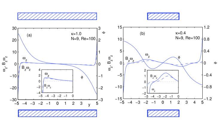
Figure 8: Spanwise cuts, $x\!=\!z\!=\!0$, of vorticity, $\omega_{z}$ (left axis, solid), magnetic field multiplied by vorticity, $B_{z}\omega_{z}$ (left axis, dashed), and electric potential,$\phi$ (right axis), for $\kappa=1$(plot $a$) and $0.4$(plot $b$); $N=9$, $Re=100$. Filled rectangles at top and bottom show schematically magnets.

The behavior of vorticity, $\omega_{z}\!\approx\!-\partial u_{x}/\partial y$, can be easily understood from the spanwise deformation of the streamwise velocity, i.e. $M$-shaped velocity profile, Fig. 5($c$). Such a profile is characterized by two jets sidelong streamlining the magnetic obstacle, and each jet has the internal and external slope, hence, the vorticity alternates its sign by passing the velocity maximum of the jet. The steepness of the external side of the jet is significantly higher than that of the internal side, especially for the larger $\kappa$ because the external slope is adjoined with no-slip sidewalls. Fig. 8 shows that the sidewalls vorticity, i.e. the external slope vorticity, is larger by an order of magnitude than the vorticity adjoining the center, i.e. the internal slope vorticity. To stress this fact, Fig. 8 shows both global and zoomed (insets) views for $\omega_{z}$ and $B_{z}\omega_{z}$.

When the spanwise variation of the magnetic field $B_{z}(y)$ is weak, e.g. for the broad magnet ($\kappa=1$) shown in Fig. 8($a$), the product of $B_{z}\omega_{z}$ reflects completely the quantitative difference in $\omega_{z}$ taken on the internal and external jet sides. Because the external $\omega_{z}$ is much higher than the internal $\omega_{z}$, the distribution of $\phi$ is determined mainly by the vorticity generated on sidewalls rather than by that produced inside the obstacle. Therefore, the negative (positive) external $\omega_{z}$ induces strong positive (negative) potential on the sidewalls, and $\phi(y)$ drops monotonically along the $y$-axis, i.e. the spanwise electrostatic field $E_{y}=-\partial\phi/\partial y$ is always positive and does not change its sign between sidewalls.

If the magnetic field is perfectly uniform along the $y$-axis, the electric potential distribution is completely governed by the sidewalls vorticity, and the alternating vorticity on the internal slopes of the $M$-shaped profile does not contribute to $\phi(y)$ even at large interaction parameter $N$. As a result, the electrostatic field ${\bf E}\approx(0,E_{y},0)$ in the region of magnetic obstacle is always directed opposite to electromotive force, ${\bf u\times B}\approx(0,-u_{x}B_{z},0)$. By braking the flow, streamwise velocity $u_{x}$ and spanwise field $E_{y}$ accordingly approach zero by keeping their signs. A stagnant region can develop where streamwise velocity is small but still positive because the electric field is always in the same direction. Therefore, recirculation is impossible.

Let us consider the case when the magnetic field intensity, $B_{z}(y)$, drops from the center to sidewalls. Here, the high vorticity generated by sidewalls in the product of $B_{z}\omega_{z}$ is suppressed by a low intensity of the magnetic field. This is shown by the middle magnet ($\kappa=0.4$), Fig. 8($b$)), the corresponding $B_{z}(y)$ is presented by dashed lines in Fig. 3($c$). The product of $B_{z}\omega_{z}$ resembles the $\omega_{z}(y)$ behavior inside the magnetic obstacle, since there $B_{z}(y)\approx\mbox{const}$, i.e. the internal vorticity is well presented in $B_{z}\omega_{z}$. Outside the obstacle, $B_{z}(y)$ rapidly decreases, so the external vorticity is remarkably weakened: as follows from Fig. 8($b$), the dashed $B_{z}\omega_{z}$ curve diverges from the solid $\omega_{z}$ curve. The largest difference between $\omega_{z}$ and $B_{z}\omega_{z}$ are present on sidewalls where the external vorticity is very high due to no slip boundary conditions, while $B_{z}\omega_{z}$ at $|y|=L_{y}$ is of the same magnitude because its alternating extrema at $|y|\approx M_{y}$ correspond with borders of the magnet. Therefore, the dependence of $\phi(y)$ is allowed to be influenced by the internal slopes of the $M$-shaped profile, which produces extrema on $\phi(y)$ at $|y|\approx M_{y}$ alternating with the sign of $\phi$ on sidewalls. These internal extrema on $\phi(y)$ reverse the spanwise electric field i.e. $E_{y}=-\partial\phi/\partial y$ becomes negative inside a finite magnetic obstacle.

The reverse spanwise electrical field appearing for spanwise decaying magnetic field is a necessary but not sufficient condition for the appearance of reverse flow. It is a necessary condition, because otherwise no Lorentz force pointing in negative $x$-direction would appear. This becomes clear looking at equations (1) and (2) for Lorentz force and current density: ${\bf j}\times{\bf B}=-\nabla\phi\times{\bf B}-B^{2}{\bf u}+({\bf u}\cdot{\bf B}){\bf B}$. Considering again the central spanwise cut, $x=z=0$, where ${\bf B}=(0,0,B_{z})$, ${\bf u}\approx(u_{x},0,0)$ and ${\bf j}\approx(0,j_{y},0)$, one can write the $x$-component of the Lorentz force as follows: $({\bf j}\times{\bf B})_{x}\approx j_{y}B_{z}=E_{y}B_{z}-B_{z}^{2}u_{x}$. The third term has vanished, the second term corresponds to a frictional force proportional to the actual velocity. The only term, which can provide a driving force for the reverse flow is the first term, and this only then when $E_{y}$ is negative, i.e. when a reverse spanwise electrical field exists. Only the existence of a reverse spanwise electrical field is not sufficient to drive reverse flow, because it has to reach a minimal strength. This becomes clear from the $y$-component of Ohm’s law for the electrical current density at the central spanwise cut: $j_{y}=E_{y}-u_{x}B_{z}$. To see this, one needs an additional information concerning the global behavior of the electrical current in our system. The electrical current is organized in two horizontal loops, with a strong negative spanwise current (i.e. $j_{y}<0$) directly under the magnet, which divides at the sidewalls into one loop before the magnet and the other behind the magnet (see figures 16, 17 and 18 of our former paper Votyakov & Zienicke (2007)). The sign of $j_{y}$ does not change, when the interaction parameter is increased. When $E_{y}$ just changes sign at a certain value of $N$ at the start of electric field reversal, $-u_{x}B_{z}$ has to be negative. This is only possible for (still) positive $u_{x}$, and consequently $N$ has to be further increased until the reverse spanwise electrical field becomes so strong that it equals the value of $j_{y}$. This characterizes, in fact, the critical $N_{c,m}$, for which the velocity $u_{x}$ is exactly zero. Let us denote this value of the reverse spanwise electrical field by $E_{y,c}$. A further increase of the interaction parameter makes $E_{y}$ stronger negative than $j_{y}$ with the consequence that $u_{x}$ has to be smaller than zero, which is equivalent to the existence of reverse flow and recirculation. Thus, summing all up, the role of spanwise magnetic field gradient is to suppress the external vorticity and promote the internal vorticity in the product of ${\bf B\cdot\omega}$. When by a further increase of the interaction parameter the internal spanwise electrostatic field is reversed stronger than the critical $E_{y,c}$, the recirculation appears.

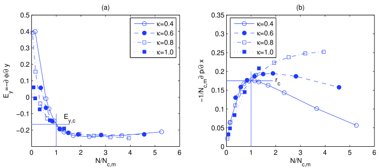
Figure 9: For various magnetic field configurations, $\kappa=0.4$ (open circles), 0.6 (filled circles), 0.8 (open squares), 1.0 (filled squares), the dependencies on $N/N_{c,m}$ in the center of magnetic obstacle, $x\!=\!y\!=\!z\!=\!0$ of the spanwise electrostatic field, $E_{y}\!=\!-\partial\phi/\partial y$, (plot $a$), and the normalized resistance to the flow, $r=(-\partial p/\partial x)/N_{c,m}$, (plot $b$).

Fig. 9($a$) shows $E_{y}=-\partial\phi/\partial y$ for the different magnets taken in the center of the magnetic gap, $x\!=\!y\!=\!z\!=\!0$, as a function of the interaction parameter $N$ normalized with the critical value $N_{c,m}$. Letting the appearance of recirculation be the referred flow pattern, the ratio $N/N_{c,m}$ characterizes the power of recirculation for various $\kappa$. One can see that the curves are close to each other when $N/N_{c,m}\gtrsim 1$. Moreover, by taking $N/N_{c,m}=1$ one finds that the critical $E_{y,c}\approx-0.17$ is independent of $\kappa$. That is, the critical magnitude of the spanwise electrostatic field, $E_{y,c}$ is a universal parameter which is the same for different magnetic field configurations. This fact is clear because $B_{z}=1$ and $j_{y}=E_{y,c}$ when the recirculation starts, i.e. $u_{x}\!=\!u_{y}\!=\!0$. So, $E_{y,c}$ is indeed the critical braking Lorentz force because $F_{L,x}=j_{y}B_{z}=E_{y,c}$.

Let $r\!=\!-(\partial p/\partial x)/N_{c,m}$ at $x\!=\!y\!=\!z\!=\!0$ be the resistance to the flow inside the magnetic obstacle. At the beginning of recirculation the Navier-Stokes equation is simplified up to $\partial p/\partial x+N_{c,m}E_{y,c}=0$, so $r_{c}=-E_{y,c}$. The behavior of $r$ as a function of $N/N_{c,m}$ for various $\kappa$ is shown in Fig 9($b$). One can see that the change of the flow regime is accompanied by the change of the slope in the resistance of $r(N/N_{c,m})$. For those $\kappa$ where the sidewall influence is insignificant, the appearance of recirculation at $N/N_{c,m}\gtrsim 1$ results in a drop of the resistance despite the fact that $N$ increases.

The second effect of a drop in the resistance due to magnetic recirculation has the same explanation as the drag crisis well known in ordinary hydrodynamics. It appears in the wake of a circular cylinder when the boundary layer on the cylinder surface undergoes a transition from the laminar to turbulent mode. It causes a substantial reduction in the drag force analogous to that in the wake of the magnetic obstacle.

3.5 Similarity of MHD flows inside the magnetic obstacle

As follows from Eq.(1) the viscous force $\Delta{\bf u}$ is scaled by Reynolds number $Re$, therefore at high $Re$ and far from the walls it plays a minor role. As a result the flow must be governed by the interaction parameter $N$ defining the ratio between magnetic and inertial forces. This peculiarity was marked already in Votyakov & Zienicke (2007) by comparing experimental and numerical electric potential distributions found at different $Re$ and similar $N$.

In the present paper, Fig. 10 demonstrates the same behavior for the broad (curves $1$ and $3$) and middle (curves $2$) magnet. Solid and dashed curves $1,2$ have the same $N$ but $Re=100$ for solid and $Re=400$ for dashed lines.

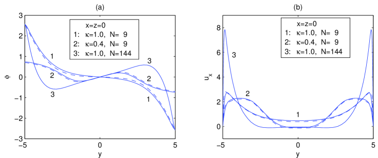
Figure 10: Spanwise dependence ($x\!=\!z\!=\!0$) of electric potential (plot $a$) and streamwise velocity (plot $b$) for the broad ($\kappa=1.0,\;N_{c_{m}}=109$, solid and dashed curves $1,3$) and middle ($\kappa=0.4,\;N_{c_{m}}=6.8$, solid and dashed curves $2$) magnetic obstacle. $N=9$ (curves $1,2$) and 144 (curves $3$), $Re=100$ (solid) and 400 (dashed lines). Notice that for the curves $2$ and $3$ the constrainment factors $\kappa$ are different, while the relations $N/N_{c,m}\approx 1.32$ are equal.

It is expected after discussing Fig. 9 that the results given in Fig. 10 are similar even for different constrainment factors $\kappa$ and interaction parameters $N$ provided the corresponding ratios $N/N_{c,m}$ are equal. Curve 2 for the middle magnet is plotted for $N=9$, i.e. $N/N_{c,m}(\kappa=0.4)=9/6.8=1.32$ and curve $3$ for the broad magnet – for $N=144$, i.e. $N/N_{c,m}(\kappa=1.0)=144/109=1.32$. One can see that in the central part $|y|\lesssim 2$ being approximately the spanwise dimension of the less magnet ($M_{y}=0.4\times 5=2$) both electric potential ($a$) and streamwise velocity ($b$) are also close to each other, cf. curves $2$ and $3$.

3.6 3D peculiarities of the flow

Fig. 11 shows different 3D space perspective views of the six-fold vortex pattern for the middle magnet ($\kappa=0.4$), $N=16$, and $Re=196$. For easy visualization, plot $a$ shows the $XY$ projection of all vortices, i.e. magnetic, connecting, and attached, while other plots present only part of the recirculation. Plot $b$ shows the $XZ$ projection for magnetic and attached vortices, plots ($c-d$) are both $YZ$ projections of the magnetic, and attached vortices, correspondingly.

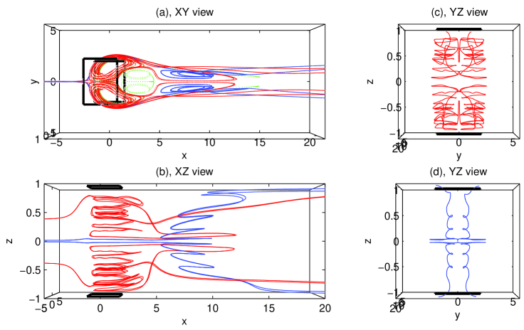
Figure 11: Perspective projection of 3D vortex disposition for middle magnet and $N\!=\!16$, $Re\!=\!196$: $XY$ view, magnetic, connecting and attached vortices ($a$), $XZ$ view, magnetic and attached vortices ($b$), $YZ$ view, magnetic vortices ($c$), $YZ$ view, attached vortices ($d$).

The following 3D features are observed in Fig. 11: (i) a helical motion inside every vortex; (ii) the axes of rotation of the magnetic vortices are parallel to the lines of external magnetic field; (iii) the two magnetic vortices are closely adjoined to each other and taken together they form a barrel extending in its central part and located mainly between magnetic poles; (iv) two helices of attached vortices are not adjoined and are arched along $x$-direction.

Additionally, Fig. 12 present flow streamlines constructed from $u_{y}$ and $u_{z}$ components of velocity field for few characteristic vertical slices: at front of the magnet ($x\!=\!-4$, plot $a$), and the vertical cuts of magnetic ($x\!=\!0$, plot $b$), connecting ($x\!=\!4$, plot $c$) and attached ($x\!=\!8$, plot $d$) vortices. These ($u_{y}$, $u_{z}$) streamlines are not real moving lines of fluid particles in the vertical slices, because the particles have also the $u_{x}$ velocity component. Instead, these streamlines are to show ascending and descending paths of fluid particles in vertical slices as projection.

At $x=-4$, Fig. 12$a$, one observes the braking effect of the Lorentz force making the flow streamlines diverge from the central point $y=z=0$, where the greatest change of $\partial u_{x}/\partial x=-(\partial u_{y}/\partial y+\partial u_{z}/\partial z)$ occurs. Because the $u_{x}$ component is not involved in the plot, this effect looks as the source of the flow. Also there is a motion in $z$ direction caused by a tendency to form Hartmann layers, see Votyakov & Zienicke (2007).

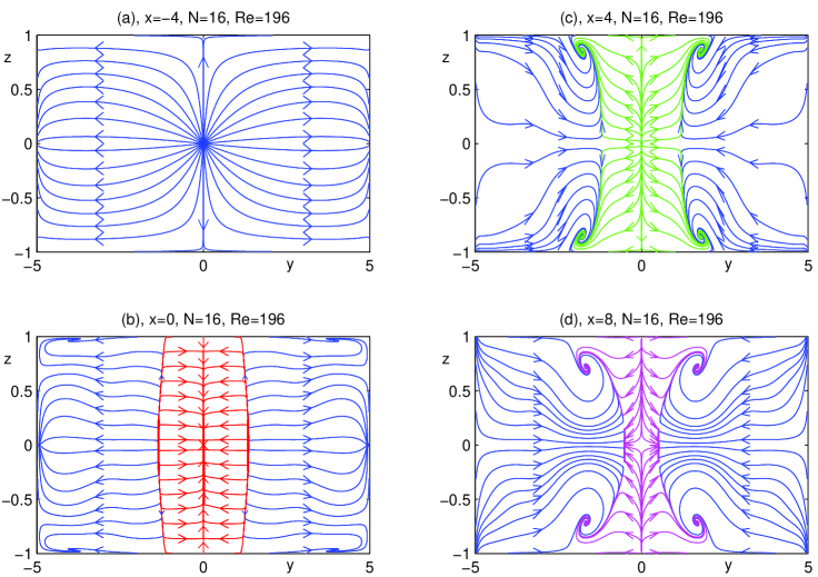
Figure 12: Flow streamlines constructed from $u_{y}$, $u_{z}$ velocity components in vertical slices $x=-4(a)$, 0($b$), 4($c$), and 8($d$); $N\!=\!16$, $Re\!=\!196$.

At $x=0$, Fig. 12$b$, one firstly notices the abrupt change of the motion in $y$ direction at $|y|\approx 2$. This helps us to see the vertical borders of the magnetic vortices where the $u_{y}$ reverse its sign. Moreover, a barrel shape of the magnetic vortex dipole can be clearly seen. Directions of arrows on the flow streamline demonstrate a drift of the flow from top/bottom walls towards the center inside the magnetic vortices, and a drift in the opposite direction outside. Such a drift is a reflection of helical motion which can be seen in perspective in Fig. 11.

Similar to Fig. 12$b$, sharp borders between the main flow and connecting ($x=4$, Fig. 12$c$) and attached ($x=8$, Fig. 12$d$) vortices are observed. One also observes a remarkable vertical drift to and from the top and bottom walls depending on the direction of horizontal rotation. The vertical drift at $x=4$ and $x=8$ is more pronounced than that of at $x=0$ because the magnetic field has a much larger intensity in the case of $x=0$. The new phenomena compared to Fig. 12$b$ are swirls in the corners of the duct shown in plots ($c,d$). Similar swirls can also appear when a MHD flow has no recirculation. They arise due to the inertial force and destruction of Hartmann layers resulting from a decline of the magnetic field, see Votyakov & Zienicke (2007).

The vertical drifts shown in Fig. 12$b-d$ are caused by rotation of the fluid and can be understood as a manifestation of the hydrodynamic Ekman pumping effect, see e.g. Davidson (2001). There are six rotating columns in the MHD flow studied here, and each one has its own primary horizontal motion and secondary vertical drift. Taken all together it gives rise to the helical motion clearly observed in Fig. 11.

The whole 3D space trajectory for the infinitesimally small volume of the fluid – a fluid particle – can now be described in the following way. Far upstream from the magnetic system, the particle moves straight under the pressure gradient. Approaching the region of influence of the magnetic obstacle, the particle turns aside towards the closest corner due to the action of the braking Lorentz force and reaches a boundary layer. If the particle is not captured by recirculation, it then passes the region of the magnetic obstacle in the bulk of two jets sidealong streamlined the obstacle. If the particle is captured by recirculation, it first goes down (up) from the top (bottom) towards the middle plane in the helix of the magnetic vortex. In the middle plane, this trajectory is taken by the helix of the closest connecting vortex and passes helically towards the top (bottom) wall to come again to the boundary layer and dissipate the kinetic energy. Then, the particle can be caught by the helix of the attached vortex and be drifted slowly to the middle plane where it finally becomes free to go downstream from the magnet.

Recirculation under magnetic poles brings new details into top and bottom boundary layers perpendicular to the magnetic field. These layers are Hartmann layers in the case of a constant magnetic field, Ekman layers in the case of an axisymmetric rotating flow bounded by a fixed horizontal plate, and Ekman-Hartmann layers when the axisymetric rotating flow is subject to a constant vertical magnetic field, Acheson & Hide (1973), Desjardins et al. (1999). We checked velocities profiles $u_{x}(z)$ in the region of magnetic vortices and found no satisfactory agreement with the current theory for Ekman-Hartman rotating flows. The reasons for this disagreement are probably that the recirculation induced by a heterogenous external magnetic field shows details which are not compatible with the present analytic theory: (i) the rotating flow is not axisymmetric, (ii) neither magnetic field nor angular rotation are constant, (iii) this is a system of six rotating flows. The quantitative analysis of these layers requires further detailed investigation. At the moment we can conclude only that these layers are important to stabilize recirculation even at high Reynolds numbers as shown in next Section.

3.7 Recirculation in a 3d flow versus a vortex generation in a 2D flow

This paper is devoted to a stationary 3D MHD flow. Recently, Cuevas et al. (2006a) have reported a vortex generation in a 2D flow induced by a magnetic obstacle. In this Section, we discuss how their 2D results are related to our 3D results.

In our opinion, it is an open question on how to build a 2D model at high $Re$. Two-dimensionality assumes that the flow rate is kept constant in the plane under consideration. This assumption is certainly wrong in the case of a local magnetic field, where Hartmann layers are formed (destroyed) under inward (outward) magnetic field gradient, i.e. streamwise velocity profile in the transverse direction is becoming more (less) flat, therefore the fluid must go out of (go into) the plane, see discussion about Fig.8,9 given by Votyakov & Zienicke (2007).

On one hand, the friction imposed by a no-slip wall stabilizes a flow because it provides a sink for kinetic energy. For instance, in ordinary hydrodynamics there are numerous experiments which illustrate that the confinement of the endplates increases the stability of the wake, see e.g. Shair et al. (1963), Nishioka & Sato (1974), Gerich & Eckelmann (1982), Lee & Budwig (1991). These examples include the delay of the critical Reynolds number for vortex shedding and the extension of the Reynolds number range for a 2D laminar shedding.

On the other hand, the case of a MHD flow under a local magnetic field always requires to take into account top and bottom endplates because these plates carry magnetic poles. In reality, one can increase the distance between poles to have more two-dimensionality in the middle plane, but this automatically decreases the degree of space heterogeneity of the external magnetic field. So, it becomes an issue whether it is practically possible to design a strongly heterogenous magnetic field having a large distance between magnetic poles.

There is a method to take no-slip top/bottom plates into consideration by means of the Hartmann friction term, see e.g. Lavrentiev et al. (1990). This assumption has been used also by Cuevas et al. (2006a). However, this averaged approach is well validated only in the case of a small flow rate, i.e. low $Re$, even when the magnetic field is not strongly varying. It follows from the fact that past the magnetic obstacle the Hartmann friction takes a form of the Hele-Shaw friction based on the assumption that velocity is parabolic along the $z$-axis. This is well validated only for viscous flows where the vorticity advection does not play a significant role, Riegels (1938). The formal vertical Hele-Shaw friction term inserted into the 2D Navier-Stokes equations does not describe quantitatively the behavior of the system with high $Re$. We believe that this friction has no significant influence when the advection is strong.

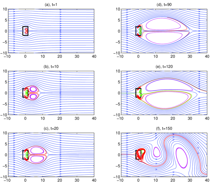
Figure 13: Flow streamlines in a 2D nonsteady free flow: $t=1(a)$, 10($b$), 20($c$), 90($d$), 120($e$), 150($f$); ${\bf u(r)}|_{t=0}=(1.5,0)$, $N\!=\!30$, $Re\!=\!100$.

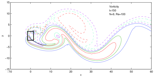
Figure 14: Vorticity field corresponding to Fig. 13($f$). Dashed lines are plotted for negative, and solid lines are plotted for positive vorticity.

Nevertheless, one can consider mathematically what happens in a 2D free (no side walls) MHD flow where the flow rate is kept constant. This mathematical problem has been addressed by Cuevas et al. (2006a).

The cited 2D MHD flow had no walls, and, hence, no sinks for kinetic energy except an internal viscosity which is negligible when $Re$ is high. In such a flow, any vortex pattern cannot be stabilized, and one would not observe any stationary recirculation. Instead one obtains the nonsteady vortex generation, hence, it is worth to discuss a developing flow, i.e. the flow starting from the constant velocity field ${\bf u(r)}|_{t=0}=(u_{x},0)$. We have performed a few runs of 2D simulation in order to reproduce results of Cuevas et al. (2006a) and find out whether the six-fold vortex pattern shown in Fig. 1($b$) is of general matter. These results are presented in Fig. 13.

One observes, at the initial times, subsequently symmetric magnetic vortices (Fig. 13($a$)), and then a six-vortex pattern (Fig. 13($b,c$)). This pattern quickly grows in size due to inertia, (Fig. 13)($b,c,d$), in such a way that attached vortices gradually swell and reach a dimension much larger than that of magnetic and connecting vortices. When attached vortices exceed their critical size, they become unstable and lose symmetry, Fig. 13($e$). This gives rise to the Karman vortex street, Fig. 13($f$), illustrated also by a vorticity contour plot in Fig. 14. The Karman vortex street has been reported already by Cuevas et al. (2006a), while the preceding temporal evolution, Fig. 13($a-f$), is explained here for the first time.

It is known that the attached vortices in the flow past a solid body can be discovered at any Reynolds number $Re$ at the initial instance of time before vortex shedding starts. One can see that the same situation takes place in an initial flow past the magnetic obstacle. The difference is that instead of just attached vortices one can observe a six-fold vortex pattern developing from the recirculation under the magnetic gap.

4 Conclusions

We have reported the results of a 3D numerical study about a stationary liquid metal flow in a rectangular duct under the influence of an external magnetic field. The interaction parameter $N$, Reynolds number $Re$ as well as magnetic field configuration have been systematically varied. Whenever it has been possible, the numerical results have been quantitatively compared with experimental ones.

First, an analytical, physically consistent and simple model for the external magnetic field has been derived. Parameters of the model are geometric dimensions of a region occupied by external magnets. This model has been successfully verified by comparing with experimentally measured data and then used through the paper by varying the constrainment factor, $\kappa=M_{y}/L_{y}$, the ratio between spanwise dimension of the magnet, $2M_{y}$, and width of the duct, $2L_{y}$.

One can classify the following three typical flow structures into which a stationary MHD flow is organized, depending on the interaction parameter $N$ as well as spanwise magnetic field heterogeneity.

The first structure, attributed to low degree of field heterogeneity, is characterized by the significant electromotive force which opposes the electrostatic field. The characteristic pattern for this case is the Hartmann flow. If magnetic field is uniform, this regime takes place at all $N$, otherwise it is realized at such $N$ when the field heterogeneity is not strong manifested.

The second stationary structure is perfectly observed for the fringing magnetic field, i.e. when the intensity of transverse magnetic field is varied slowly in the spanwise and strongly in the streamwise direction. The flow pattern is given by the $M$-shaped streamwise velocity profile without recirculation inside the magnetic gap. Here, the electromotive force and the electrostatic field can either be opposed or be in the same direction, but the direction of the electromotive force is always in the direction of the electric current. The loops of the electric current are located mainly in the horizontal plane.

The decisive condition for the appearance of the third flow structure is a strong spanwise variation of the magnetic field which induces recirculation inside the magnetic obstacle. The recirculation starts when the reverse electrostatic field prevails a critical value. Here, the electromotive force is opposed to the electrostatic field and the direction of the electric current. For this recirculation regime, the intensities of the reverse flow, obtained in 3D numerically and by physical experiments have been compared, and a good agreement has been observed.

The existence regions of stable stationary flow patterns, that is the dependence of the critical interaction parameter, $N_{c,m}$, to induce recirculation on the constrainment factor, $\kappa$, has been calculated and discussed. It has been made clear that no recirculation is possible for perfectly spanwise uniform external magnetic field. Moreover, the MHD flows for various $\kappa$ have been shown to be similar provided they are of the same ratio $N/N_{c,m}$.

Finally, 3D features of the flow under consideration have been discussed and it has been demonstrated that the magnetic vortices are stable in their disposition. This is contrary to a $2D$ numerical study where the stationary recirculation is possible only in a creeping flow while at higher flow rate the recirculation develops a vortex shedding. Nevertheless, one can see all these vortex patterns in a 2D nonsteady flow at initial times.

We do not want to close this work without some hypotheses on the nature of the transitions that we have found in this system, namely, (1) the transition between streamlining flow and the flow with magnetic vortices when $N_{c,m}$ and $\kappa$ are varied, and (2) the transition from the two-vortex pattern (only magnetic vortices) to the six-vortex pattern (magnetic, connecting and attached vortices) when the Reynolds number is varied. The first transition has a high probability to be a topological change of the same solution, which is stable in the whole space of initial conditions. Increase of the strength as well as the increase or decrease of the spanwise inhomogeneity of the magnetic field seem us to be topological changes of the force field resulting in a topological change of the stationary stable solution. This would be consistent with the fact, that we never found the different flow patterns coexisting for the same parameter pair ($N_{c,m}$,$\kappa$). The second transition mentioned is to our opinion analogous to the appearance of attached vortices behind a solid obstacle as known from usual hydrodynamics. The magnetic vortices act as an obstacle for the flow. For increasing Reynolds number a shear instability arises resulting into the formation of attached vortices, which for consistence of the flow have to be accompanied by the connecting vortices. These impressions on the questions of stability, that we got from our research on the considered system, nevertheless, remain to be proved rigorously.

Appendix A Indefinite integrals

We take the following notations: ${\bf r}=(x,y,z)$, $\;{\bf r^{\prime}}=(x^{\prime},y^{\prime},z^{\prime})$, $\;\Delta r=|r-r^{\prime}|=\left[\Delta x^{2}+\Delta y^{2}+\Delta z^{2}\right]^{1/2}$ and $\Delta x=x-x^{\prime}$,$\;\Delta y=y-y^{\prime}$, $\;\Delta z=z-z^{\prime}$. Then, the indefinite integration over $z^{\prime}$ gives

$$\Phi^{(z)}(x,y,z,x^{\prime},y^{\prime},z^{\prime})=\int\frac{dz^{\prime}}{|\bf{r-r^{\prime}}|}=-\mbox{arctanh}\left[\frac{\Delta z}{\Delta r}\right],$$ (8)

the indefinite integration over $z^{\prime},y^{\prime}$ gives

$$\Phi^{(z,y)}(x,y,z,x^{\prime},y^{\prime},z^{\prime}) = \int\frac{dy^{\prime}dz^{\prime}}{|\bf{r-r^{\prime}}|}=-\Delta x\,\mbox{arctan}\left[\frac{\Delta y\Delta z}{\Delta x\Delta r}\right]$$ (9)

$$+ \Delta y\,\mbox{arctanh}\left[\frac{\Delta z}{\Delta r}\right]+\Delta z\,\mbox{arctanh}\left[\frac{\Delta y}{\Delta r}\right],$$

and finally the indefinite integration over $z^{\prime},y^{\prime},x^{\prime}$ gives

$$\Phi^{(z,y,x)}(x,y,z,x^{\prime},y^{\prime},z^{\prime}) = \int\frac{dx^{\prime}dy^{\prime}dz^{\prime}}{|\bf{r-r^{\prime}}|}$$ (10)

$$= \frac{1}{2}\Delta x^{2}\arctan\left[\frac{\Delta y\Delta z}{\Delta x\Delta r}\right]-\Delta y\Delta z\,\mbox{arctanh}\left[\frac{\Delta x}{\Delta r}\right]$$

$$+ \frac{1}{2}\Delta y^{2}\arctan\left[\frac{\Delta x\Delta z}{\Delta y\Delta r}\right]-\Delta x\Delta z\,\mbox{arctanh}\left[\frac{\Delta y}{\Delta r}\right]$$

$$+ \frac{1}{2}\Delta z^{2}\arctan\left[\frac{\Delta x\Delta y}{\Delta z\Delta r}\right]-\Delta x\Delta y\,\mbox{arctanh}\left[\frac{\Delta z}{\Delta r}\right].$$

To confirm, one can use a commercial program, e.g. Mathematica, to analytically differentiate (10) back and get (8) finally. The original way to calculate (8)-(10) is quite cumbersome, and is not provided here.

References

- Acheson & Hide (1973) Acheson, D. J. & Hide, R. 1973 Hydromagnetics of rotating fluids. Reports of Progress in Physics 36, 159–221.
- Afanasyev (2006) Afanasyev, Y.D. 2006 Formation of vortex dipoles. Phys. Fluids 18, 037103.
- Alboussiere (2004) Alboussiere, Th. 2004 A geostrophic-like model for large Hartmann number flows. J. Fluid. Mech. 521, 125–154.
- Andreev et al. (2007) Andreev, O., Kolesnikov, Yu. & Thess, A. 2007 Experimental study of liquid metal channel flow under the influence of a non-uniform magnetic field. Phys. Fluids 19, 039902.
- Cuevas et al. (2006a) Cuevas, S., Smolentsev, S. & Abdou, M. 2006a On the flow past a magnetic obstacle. J. Fluid. Mech. 553, 227 – 252.
- Cuevas et al. (2006b) Cuevas, S., Smolentsev, S. & Abdou, M. 2006b Vorticity generation in creeping flow past a magnetic obstacle. Phys. Rev. E 74, 056301.
- Davidson (1999) Davidson, P. 1999 Magnetohydrodynamics in Materials Processing. Annual Review of Fluid Mechanics 31, 273–300.
- Davidson (2001) Davidson, P. A. 2001 An introduction to Magnetohydrodynamics. Cambridge University Press.
- Desjardins et al. (1999) Desjardins, B., Dormy, E. & Grenier, E. 1999 Stability of mixed Ekman-Hartmann boundary layers. Nonlinearity 12, 181–199.
- Gelfgat & Olshanskii (1978) Gelfgat, Y. M. & Olshanskii, S. V. 1978 Velocity structure of flows in non-uniform constant magnetic fields. ii. experimental results. Magnetohydrodynamics 14, 151–154.
- Gelfgat et al. (1978) Gelfgat, Y. M., Peterson, D. E. & Shcherbinin, E. V. 1978 Velocity structure of flows in nonuniform constant magnetic fields 1. numerical calculations. Magnetohydrodynamics 14, 55–61.
- Gerich & Eckelmann (1982) Gerich, D. & Eckelmann, H. 1982 Influence of end plates and free ends on the shedding frequency of circular cylinders. J. Fluid. Mech. 122, 109–121.
- Griebel et al. (1995) Griebel, M., Dornseifer, T. & Neunhoeffer, T. 1995 Numerische Strömungssimulation in der Strömungsmechanik. Braunschweig: Vieweg Verlag.
- Jackson (1999) Jackson, J.D. 1999 Classical Electrodynamics, Third Edition. New York, NY, U.S.A.: Wiley.
- Kit et al. (1970) Kit, L. G., Peterson, D. E., Platnieks, I. A. & Tsinober, A. B. 1970 Investigation of the influence of fringe effects on a magnetohydrodynamic flow in a duct with nonconducting walls. Magnetohydrodynamics 6, 485–491.
- Kunstreich (2003) Kunstreich, S. 2003 Electromagnetic stirring for continuous casting. Rev. Met. Paris (4), 395–408.
- Lavrentiev et al. (1990) Lavrentiev, I.V., Molokov, S.Yu., Sidorenkov, S.I. & Shishko, A.Ya 1990 Stokes flow in a rectangular magnetohydrodynamic channel with nonconducting walls within a nonuniform magnetic field at large Hartmann numbers. Magnetohydrodynamics 26 (3), 328–338.
- Lee & Budwig (1991) Lee, T. & Budwig, R. 1991 A study of the effect of aspect ratio on vortex shedding behind circular cylinders. Physics of Fluids 3, 309–315.
- Moreau (1990) Moreau, R. 1990 Magnetohydrodynamics. Dordrecht: Kluwer Academic Publishers.
- Nishioka & Sato (1974) Nishioka, M. & Sato, H. 1974 Measurements of velocity distributions in the wake of a circular cylinder at low reynolds numbers. J. Fluid. Mech. 65, 97–112.
- Riegels (1938) Riegels, F. 1938 Zur Kritik des Hele-Shaw-Versuchs. Zeitschrift fur Angewandte Mathematik und Mechanik 18 (2), 95–106.
- Roberts (1967) Roberts, P. H. 1967 An introduction to Magnetohydrodynamics. New York: Longmans, Green.
- Shair et al. (1963) Shair, F. H., Grove, A. S., Petersen, E. E. & Acrivos, A. 1963 The effect of confining walls on the stability of the steady wake behind a circular cylinder. J. Fluid. Mech. 17, 546–550.
- Shercliff (1962) Shercliff, J. A. 1962 The theory of electromagnetic flow-measurement. Cambridge University Press.
- Sterl (1990) Sterl, A. 1990 Numerical simulation of liquid-metal MHD flows in rectangular ducts. J. Fluid. Mech. 216, 161–191.
- Takeuchi et al. (2003) Takeuchi, S., Kubota, J., Miki, Y., Okuda, H. & Shiroyama, A. 2003 Change and trend of molten steel flow technology in a continous casting mould by electromagnetic force. In Proc. EPM-Conference. Lyon, France.
- Tananaev (1979) Tananaev, A. B. 1979 MHD duct flows. Moscow: Atomizdat.
- Thess et al. (2006) Thess, A., Votyakov, E. V. & Kolesnikov, Y. 2006 Lorentz Force Velocimetry. Phys. Rev. Lett. 96, 164501.
- Voropayev & Afanasyev (1994) Voropayev, S. I. & Afanasyev, Y. D. 1994 Vortex Structures in a Stratified Fluid. London: Chapman and Hall.
- Votyakov et al. (2007) Votyakov, E. V., Kolesnikov, Y., Andreev, O., Zienicke, E. & Thess, A. 2007 Structure of the wake of a magnetic obstacle. Phys. Rev. Lett. 98 (14), 144504.
- Votyakov & Zienicke (2007) Votyakov, E. V. & Zienicke, E. 2007 Numerical study of liquid metal flow in a rectangular duct under the influence of a heterogenous magnetic field. Fluid Dynamics & Materials Processing 3 (2), 97–113.