Quantification of discreteness effects in cosmological $N$-body simulations:
II. Evolution up to shell crossing

Abstract

Abstract

We apply a recently developed perturbative formalism which describes the evolution under their self-gravity of particles displaced from a perfect lattice to quantify precisely, up to shell crossing, the effects of discreteness in dissipationless cosmological $N$-body simulations. We give simple expressions, explicitly dependent on the particle density, for the evolution of power in each mode as a function of red-shift. For typical starting red-shifts the effect of finite particle number is to slow down slightly the growth of power compared to that in the fluid limit (e.g. by about ten percent at half the Nyquist frequency), and to induce also dispersion in the growth as a function of direction at a comparable level. In the limit that the initial red-shift tends to infinity, at fixed particle density, the evolution in fact diverges from that in the fluid limit (described by the Zeldovich approximation). Contrary to widely held belief, this means that a simulation started at a red-shift much higher than the red-shift of shell crossing actually gives a worse, rather than a better, result. We also study how these effects are modified when there is a small-scale regularization of the gravitational force. We show that such a smoothing may reduce the anisotropy of the discreteness effects, but it then increases their average effect. This behaviour illustrates the fact that the discreteness effects described here are distinct from those usually considered in this context, due to two-body collisions. Indeed the characteristic time for divergence from the collisionless limit is proportional to $N^{2/3}$, rather than $N/\log N$ in the latter case.

today

I Introduction

Cosmological $N$-body simulations have become an essential instrument in the attempt to understand the origin of large scale structure in the universe within the framework of current cosmological models (see, e.g., Efstathiou et al. (1985); Couchman (1991); Springel et al. (2005)). In this context the goal is to use such simulations to recover the clustering of dark matter, which is described by a set of coupled Vlasov-Boltzmann equations corresponding to an appropriately taken $N\rightarrow\infty$ limit. The problem of discreteness is that of the relation between these finite $N$ simulations and this continuum limit. It is a problem which is becoming rapidly of greater importance because of the need for great precision in the predictions furnished by simulations, as the observations constraining them will continue to improve in the coming years (see e.g. Huterer and Takada (2005) for a discussion of precision requirements for future weak lensing surveys).

This article is the second in a series in which we address this issue in a quantitative manner. In the first paper Joyce and Marcos (2007) we have considered only the initial conditions (IC) for such simulations, studying in detail the correlation properties of the point distributions generated with the standard algorithm used to produce them. We have identified the limit in which the continuum IC are recovered, and quantified precisely the corrections to this limit which appear at finite particle number. We have noted that there is a subtlety about how this limit is taken: the exact theoretical correlation properties of the IC in real and reciprocal space are recovered only when the limit $N\rightarrow\infty$ is taken before the limit that the initial redshift $z_{\rm init}\rightarrow\infty$. If, on the other hand, $z_{\rm init}$ is increased arbitrarily at fixed particle density, the real space correlation properties (e.g. mass variance in spheres) become dominated by those of the underlying (unperturbed) particle distribution, and thus differ completely from those of the theoretical IC. As the analysis of Joyce and Marcos (2007) is limited to the IC, no conclusion can be drawn about the relevance of these behaviours in the evolved simulations. One of our results here is that this non-interchangeability of these limits also manifests itself in the perturbative approximation to the evolution we use. As explained briefly in the conclusion of Joyce and Marcos (2007), this behavior can be understood as a manifestation of the fact that the Vlasov limit of an $N$-body system with long-range interactions is valid for sufficiently short times Braun and Hepp (1977); Spohn (1991). More specifically, this means that taking $z_{\rm init}\rightarrow\infty$, at fixed particle density, the evolution of the particle system diverges from that of the Vlasov-Poisson limit. Practically this implies that increasing the starting red-shift $z_{\rm init}$ of a simulation, keeping all else fixed, the results get worse, in the sense that they deviate further from the desired physical behaviour. This finding corrects a widespread belief (see, e.g., Scoccimarro (1998); Valageas (2002); Power et al. (2003); Tatekawa and Mizuno ) that the opposite is true, as the only envisaged error has been that due to non-linear corrections in the fluid limit (which vanish when $z_{\rm init}\rightarrow\infty$).

In this paper we pursue the study of Joyce and Marcos (2007) of discreteness effects, considering the early times dynamics of these simulations. By “early times” we mean the regime of validity of a perturbative treatment of the evolution of the full $N$-body problem which has been reported in detail in Joyce et al. (2005); Marcos et al. (2006). This corresponds to a time when the relative displacement of particles at adjacent lattice sites (which is always small compared to unity in the IC) become of order the lattice spacing, i.e., when pairs of particles first approach one another. In fluid language it corresponds approximately to “shell crossing”. The basis of the approach is a simple perturbative expansion, in the relative displacements of pairs of particles, of the force on each particle. This is in fact a standard method used to analyze phonons in a crystal, well known in solid state physics (see e.g. Pines (1963)). It leads to a 3N$\times$3N diagonalisation problem, which can be simplified using the translational symmetry of the lattice (formulated in the Bloch theorem): the eigenmodes of the displacement field are simply plane waves, with orientations and eigenvalues which can be determined numerically by diagonalising N 3$\times$3 matrices. Analysing this spectrum in the continuum limit of infinite particle density, one recovers the expected fluid behaviour in this regime. The latter is that derived through a perturbative treatment of the fluid equations in the Lagrangian formalism Buchert (1992), which gives asymptotically the Zeldovich approximation. We will refer to the discrete perturbative treatment here as “particle linear theory” (PLT) and to its fluid limit as “fluid linear theory” (FLT). By comparing evolution described by the former with the latter, we determine the discreteness effects (in the domain of validity of PLT).

That this PLT formalism can be used to this end has already been clearly demonstrated in Marcos et al. (2006). Indeed in this paper we have directly compared $N$-body simulations with both PLT and FLT and shown that the former reproduces better than the latter the real evolution. Further we have shown that PLT reproduces the full evolution extremely well at early times, and breaks down globally at roughly the same time as FLT, when the average relative displacement of particles becomes of order the interparticle distance.

In the present paper we apply this formalism in detail to quantifying discreteness effects in cosmological $N$-body simulations. To our knowledge this is the first work in which any such effect in simulations has been quantified using analytic methods. Discreteness effects have, on the other hand, been investigated, mostly numerically, by various authors (see e.g. Splinter et al. (1998); Kuhlman et al. (1996); Melott (1990); Melott et al. (1997); Diemand et al. (2004a, b); Binney (2004); Hamana et al. (2002); Baertschiger et al. (2002); Gotz and Sommer-Larsen (2003); Power et al. (2003); Wang and White ). While our results are limited to the effects which are at play up to shell crossing, they provide a complete and exhaustive understanding of this regime. As we discuss in our conclusions the physical insights gained should also be useful in attempting to understand the effects of discreteness better beyond this regime. Our results also provide an analytical description for some specific effects of discreteness which have been observed numerically, notably the effects of discreteness in breaking isotropy demonstrated by a numerical experiment in Melott et al. (1997), and the generation of structure at small scales noted in hot/warm dark matter simulations in Gotz and Sommer-Larsen (2003); Wang and White .

The paper is organized as follows. In the next section we summarize the necessary formalism which has been developed and studied in detail in Joyce et al. (2005); Marcos et al. (2006). This section is divided into three parts: the PLT formalism in full generality, the derivation of the fluid limit from it, and the specific case of evolution in an Einstein de Sitter (EdS) universe from the IC applied in cosmological simulations (using the Zeldovich approximation). For the latter case (i.e. an EdS universe) all of the cosmology dependent part of the calculations can be done analytically. It is in fact the appropriate case for almost all cosmological applications, since we are treating in practice the evolution in an epoch (before shell crossing) which corresponds to a red-shift range in which the universe, in current cosmological models, is very close to EdS. The generalization to any other cosmology (e.g. with a cosmological constant) is, however, straightforward. In Sect. III we then apply these results to quantify more precisely the effects in cosmological simulations. Specifically we calculate a simple function quantifying the modification of the average amplitude of all modes of the displacement field at given wavenumber, then a similar one for the modes of the density fluctuations and finally one quantifying the anisotropy induced in the evolution by discreteness. In the following section we study the case that there is a smooth regularization of the Newtonian potential around the origin. In particular we consider the modification induced in the quantities defined and calculated in the previous section. In Sect. V we consider the parametric and limiting behaviours of the discreteness effects which we have quantified. In particular we consider more explicitly how the effects depend on the number of particles and the recovery of the continuum limit, as well as the limit in which the initial amplitude goes to zero (i.e. the initial red-shift goes to infinity). In the final section we summarize our findings and discuss some other points. In particular we discuss the possible use of our results to correct cosmological simulations for these systematic errors due to discreteness at shell crossing. We also discuss briefly the relevance of our results to the more general problem of quantifying discreteness errors in the fully non-linear regime of these simulations.

II PLT Evolution of a perturbed lattice

In the first part of this section we present the essential elements of the PLT treatment of the early time evolution of a perturbed lattice, summarizing a much more detailed discussion which can be found in Joyce et al. (2005); Marcos et al. (2006). In the next subsection we discuss the derivation of the fluid limit of the evolution described by PLT. In the last part we then consider the specific case of evolution from a lattice as perturbed initially in cosmological simulations.

II.1 Summary of PLT formalism

The equation of motion of the particles in a dissipationless cosmological $N$-body system is (see, e.g., Efstathiou et al. (1985); Couchman (1991))

$${\ddot{\bf x}}_{i}+2H(t){\dot{\bf x}}_{i}=-\frac{1}{a^{3}}\sum_{i\neq j}\frac{Gm_{j}({\bf x}_{i}-{\bf x}_{j})}{|{\bf x}_{i}-{\bf x}_{j}|^{3}}\,.$$ (1)

Here dots denote derivatives with respect to time $t$, ${\bf x}_{i}$ is the comoving position of the $i$th particle, of mass $m_{i}$, related to the physical coordinate by ${\bf r}_{i}=a(t){\bf x}_{i}$, where $a(t)$ is the scale factor of the background cosmology with Hubble constant $H(t)=\frac{\dot{a}}{a}$. The infinite universe is treated by applying periodic boundary conditions to a finite cubic box of side $L$.

We treat first the generic case that the $N$ particles in the box are of equal mass and initially placed in any configuration which is a perturbed lattice, i.e., particles initially at the lattice sites of a perfect lattice subjected to some set of displacements. The right hand side of Eq. (1) may then be expanded perturbatively in the relative displacements of particles, about the perfect lattice configuration in which it is identically zero. Writing ${\bf x}_{i}(t)={\bf R}+{\bf u}({\bf R},t)$, where ${\bf R}$ is the lattice vector of the $i$th particle and ${\bf u}({\bf R},t)$ its displacement from R, one obtains then, at linear order in this expansion,

$${\bf{\ddot{u}}}({\bf R},t)+2H{\bf{\dot{u}}}({\bf R},t)=-\frac{1}{a^{3}}\sum_{{\bf R}^{\prime}}{\cal D}({\bf R}-{\bf R}^{\prime}){\bf u}({\bf R}^{\prime},t)\,.$$ (2)

The matrix ${\cal D}$ is known in solid state physics, for any pair interaction, as the dynamical matrix (see e.g. Pines (1963)). For gravity we have

$${\cal D}_{\mu\nu}({\bf R}\neq{\bf 0})=Gm\left(\frac{\delta_{\mu\nu}}{R^{3}}-3\frac{R_{\mu}R_{\nu}}{R^{5}}\right)$$ (3)

$${\cal D}_{\mu\nu}({\bf 0})=-\sum_{{\bf R}\neq{\bf 0}}{\cal D}_{\mu\nu}({\bf R})$$ (4)

where $\delta_{\mu\nu}$ is the Kronecker delta. Note that a sum over the copies, associated with the periodic boundary conditions, is implicit in these expressions.

The Bloch theorem for lattices tells us that ${\cal D}$ is diagonalized by plane waves in reciprocal space. We can define the Fourier transform and its inverse by

$${\bf{\tilde{u}}}({\bf k},t) =\sum_{{\bf R}}e^{-i{\bf k}\cdot{\bf R}}{\bf u}({\bf R},t)$$ (5a)

$${\bf u}({\bf R},t) =\frac{1}{N}\sum_{{\bf k}}e^{i{\bf k}\cdot{\bf R}}{\bf{\tilde{u}}}({\bf k},t)\,,$$ (5b)

where the sum in Eq. (5b) is over the first Brillouin zone (FBZ) of the lattice, i.e., for a simple cubic lattice ${\bf k}={\bf n}(2\pi/L)$, where ${\bf n}$ is a vector of integers of which each component $n_{i}$ ($i=1,2,3$) takes all integer values in the range $-N^{1/3}/2<n_{i}\leq N^{1/3}/2$.

Using these definitions in Eq. (2) we obtain

$${\bf\ddot{{\tilde{u}}}}({\bf k},t)+2H(t){\bf\dot{{\tilde{u}}}}({\bf k},t)=-\frac{1}{a^{3}}{\cal{\tilde{D}}}({\bf k}){{\bf{\tilde{u}}}}({\bf k},t)$$ (6)

where ${\cal{\tilde{D}}}({\bf k})$, the Fourier transform (FT) of ${\cal D}({\bf R})$, is a symmetric $3\times 3$ matrix for each ${\bf k}$.

Diagonalising ${\cal{\tilde{D}}}({\bf k})$ one can determine, for each ${\bf k}$, three orthonormal eigenvectors ${\bf e}_{n}({\bf k})$ and their eigenvalues $\omega_{n}^{2}({\bf k})$ ($n=1,2,3$). The latter obey a sum rule

$$\sum_{n}\omega_{n}^{2}({\bf k})=-4\pi G\rho_{0}\,,$$ (7)

where $\rho_{0}$ is the mean mass density.

Given the initial displacements and velocities at a time $t=t_{0}$, the dynamical evolution of the particle trajectories is then given as

$${\bf u}({\bf R},t)=\frac{1}{N}\sum_{{\bf k}}\left[\mathcal{P}({\bf k},t){\tilde{\bf u}}({\bf k},t_{0})+\mathcal{Q}({\bf k},t)\dot{\tilde{\bf u}}({\bf k},t_{0})\right]e^{i{\bf k}\cdot{\bf R}}$$ (8)

where the matrix elements of the “evolution operator” $\mathcal{P}$ and $\mathcal{Q}$ are

$$\mathcal{P}_{\mu\nu}({\bf k},t)= \sum_{n=1}^{3}U_{n}({\bf k},t)(\mathbf{e}_{n}({\bf k}))_{\mu}(\mathbf{e}_{n}({\bf k}))_{\nu}$$ (9a)

$$\mathcal{Q}_{\mu\nu}({\bf k},t)= \sum_{n=1}^{3}V_{n}({\bf k},t)(\mathbf{e}_{n}({\bf k}))_{\mu}(\mathbf{e}_{n}({\bf k}))_{\nu}\,.$$ (9b)

The functions $U_{n}({\bf k},t)$ and $V_{n}({\bf k},t)$ are linearly independent solutions of the mode equations

$${\ddot{f}}+2H{\dot{f}}=-\frac{\omega_{n}^{2}({\bf k})}{a^{3}}f$$ (10)

chosen such that

$$U_{n}({\bf k},t_{0})=1\,,\,\,\,\dot{U}_{n}({\bf k},t_{0})=0\,,$$

$$V_{n}({\bf k},t_{0})=0\,,\,\,\,\dot{V}_{n}({\bf k},t_{0})=1\,.$$ (11)

The determination of the evolution thus reduces to:

• 1. diagonalization of the N 3$\times$3 matrices ${\cal{\tilde{D}}}({\bf k})$, and

• 2. solution of the 3N equations (10) and (11) for the mode functions.

We note that ${\cal{\tilde{D}}}({\bf k})$, and therefore the first step, depends only on the type of lattice, and not on the cosmology. The dependence on the latter [encoded in $a(t)$] comes only in the second step, in the mode functions $U_{n}(t)$ and $V_{n}(t)$. Both steps are numerically straightforward (and require a number of operations proportional to $N$, quite feasible even with moderate computational power for $N$ as large as those used in the very largest current cosmological simulations). For certain cases, notably an EdS universe, the mode functions can be written analytically (see Marcos et al. (2006)). For completeness we give these expressions in App. A.

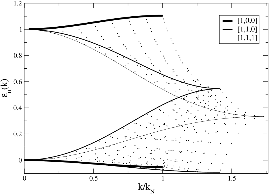
Figure 1: Normalized eigenvalues (see text) for the eigenvectors of the displacement field on a simple cubic lattice with lattice spacing $\ell$. Each point corresponds to an eigenvector labelled by a vector ${\bf k}$ in the first Brillouin zone of the lattice, and $k_{N}$ is the Nyquist frequency. The different continuous lines link ${\bf k}$ vectors oriented in the indicated directions. Note that for the $[1,O,O]$ and $[1,1,1]$ directions the two tranverse eigenmodes are degenerate because of rotational symmetry.

Details of the diagonalization of ${\cal{\tilde{D}}}({\bf k})$ are given in Marcos et al. (2006). In Fig. 1 are shown results for a $16^{3}$ simple lattice. Specifically it shows the normalized eigenvalues

$$\epsilon_{n}({\bf k})\equiv-\frac{\omega_{n}^{2}({\bf k})}{4\pi G\rho_{0}}$$ (12)

where $\rho_{0}$ is the mean mass density (arbitrarily chosen at the time $t_{0}$). These are plotted as a function of the modulus $k$ of ${\bf k}$, in units of the Nyquist frequency $k_{N}=\frac{\pi}{\ell}$ where $\ell$ is the lattice spacing. The fact that the eigenvalues at a given $k$ do not have the same value is a direct result of the anisotropy of the lattice. Shown in the plot are also lines linking eigenvectors oriented in some chosen directions. This allows one to see the branch structure of the spectrum, which is familiar in the context of analogous calculations in condensed matter physics (see e.g. Pines (1963)). The vectors ${\bf k}$ are those in the first Brillouin zone of the simple cubic lattice (as defined above).

The number of particles in the simple cubic lattice considered for the above calculation is small compared to that in current cosmological $N$-body simulations, which now attain (e.g. Springel et al. (2005)) values surpassing $1000^{3}$. While it is quite feasible, as noted above, to do these calculations for such large particle numbers, it is of little interest to do so here: the effects we are interested in depend essentially on the ratio of the wavenumber of a given mode to the Nyquist frequency. Increasing particle number only changes the density of reciprocal lattice vectors in these units (since ${\bf k}/k_{N}={\bf n}/N^{1/3}$), just filling in more densely the plot of the eigenvalues in Fig. 1 but leaving its form essentially unchanged.

In Marcos et al. (2006) we have investigated the domain of validity of PLT using numerical simulations, comparing the results of the evolution under full gravity with that obtained using the formulae just given. We have considered “shuffled lattice” IC (in which a random uncorrelated displacement is applied to each particle of the lattice, corresponding to a power spectrum $P(k)\propto k^{2}$ at small $k$), and cosmological type IC (a power spectrum $\propto k^{-2}$). In both cases the full evolution is observed to be very well approximated until a time when the average relative displacements approach the lattice spacing.

II.2 Derivation of the fluid limit (Zeldovich Approximation)

The continuum limit of this discrete analysis is easily obtained as follows. We consider the eigenmodes labelled by ${\bf k}$. Sending the particle density to infinity, at fixed mean mass density $\rho_{0}$, we approach the asymptotic behaviour seen in Fig. 1 as $k/k_{N}\rightarrow 0$. It is simple to show Marcos et al. (2006) that one has then one purely longitudinal mode (i.e. parallel to k) with $\epsilon_{n}({\bf k})=1$, and two tranverse modes with $\epsilon_{n}({\bf k})=0$. The evolution Eq. (8) may then be written

$${\bf u}({\bf R},t) = {\bf u}_{\perp}({\bf R},t_{0})U_{\perp}(t)+{\bf u}_{\parallel}({\bf R},t_{0})U_{\parallel}(t)$$

$$+{\bf v}_{\parallel}({\bf R},t_{0})V_{\parallel}(t)+{\bf v}_{\perp}({\bf R},t_{0})V_{\perp}(t),$$

where

$${\bf u}_{\parallel}({\bf R},t_{0}) =\frac{1}{N}\sum_{{\bf k}}({\tilde{\bf u}}({\bf k},t_{0})\cdot\hat{\bf k})\hat{\bf k}\ \,e^{i{\bf k}\cdot{\bf R}},$$ (14a)

$${\bf u}_{\perp}({\bf R},t_{0}) =\frac{1}{N}\sum_{{\bf k}}[{\tilde{\bf u}}({\bf k},t_{0})-({\tilde{\bf u}}({\bf k},t_{0})\cdot\hat{\bf k})\hat{\bf k}]\,e^{i{\bf k}\cdot{\bf R}},$$ (14b)

and analogously for the velocity fields, i.e., the longitudinal and transverse components of the initial displacement and velocity fields. The functions $U_{\parallel}(t)$ and $V_{\parallel}(t)$ are the linearly independent solutions of Eq. (10) for $\epsilon_{n}({\bf k})=1$ (i.e. $\omega_{n}^{2}({\bf k})=-4\pi G\rho_{0}$) ), and $U_{\perp}(t)$ and $V_{\perp}(t)$ those for $\epsilon_{n}({\bf k})=1$ (i.e. $\omega_{n}^{2}({\bf k})=0$). We have observed in Joyce et al. (2005) that, for an EdS universe, this corresponds exactly to the solution found at linear order in a perturbative treatment of the equations for a self-gravitating fluid in the Lagrangian formalism in Buchert (1992).

The solutions for the mode functions give, generically, a growing mode and a decaying mode. Since the former always dominates after a sufficient time, there is an attractive asymptotic behaviour for the general solution Eq. (II.2) which may be written in the form

$${\bf u}({\bf R},t)=g(t){\bf q}({\bf R})\,,$$ (15)

where $g(t)$ is proportional to the purely growing mode, and ${\bf q}({\bf R})$ is a longitudinal vector field. This is the Zeldovich approximation (ZA) Zeldovich (1970).

II.3 Evolution from ZA initial conditions

In cosmological simulations the ZA is used to fix the IC, usually at a time at which the universe is well approximated by an EdS cosmology. In this case we have (see App. A):

$$U_{\parallel}(t) = \frac{2}{5}\left[\frac{3}{2}\left(\frac{t}{t_{0}}\right)^{2/3}+\left(\frac{t}{t_{0}}\right)^{-1}\right]$$ (16)

$$V_{\parallel}(t) = \frac{3}{5}t_{0}\left[\left(\frac{t}{t_{0}}\right)^{2/3}-\left(\frac{t}{t_{0}}\right)^{-1}\right]$$ (17)

$$U_{\perp}(t) = 1\,,\qquad V_{\perp}(t)=3t_{0}\left[1-\left(\frac{t}{t_{0}}\right)^{-1/3}\right]\,.$$ (18)

The ZA may then be written

$${\bf u}({\bf R},t) =\frac{3}{2}\left(\frac{t}{t_{0}}\right)^{4/3}{\mathbf{g}}({\bf R},t_{0})t_{0}^{2}$$ (19a)

$${\bf v}({\bf R},t) ={\mathbf{g}}({\bf R},t_{0})t,$$ (19b)

where ${\mathbf{g}}({\bf R},t)$ and ${\bf v}({\bf R},t)$ are the peculiar gravitational acceleration field and peculiar velocity field, respectively, defined by

$${\bf v} = \dot{\bf r}-{\dot{a}}{\bf x}$$ (20)

$${\mathbf{g}} = \ddot{\bf r}-{\ddot{a}}{\bf x}=\ddot{\bf r}-\frac{{\ddot{a}}}{a}{\bf r}=a\left[\ddot{\bf u}+2\frac{{\dot{a}}}{a}\dot{\bf u}\right]\,.$$ (21)

We therefore have

$${\bf u}_{\perp}({\bf R},t_{0}) =\mathbf{0}={\bf v}_{\perp}({\bf R},t_{0})$$ (22a)

$${\bf v}_{\parallel}({\bf R},t_{0}) =\frac{2}{3t_{0}}{\bf u}_{\parallel}({\bf R},t_{0})\,.$$ (22b)

Using these specific IC in the general expression for the PLT evolution given in Eq. (8), it is simple to show that this evolution may be written in the form

$${\bf u}({\bf R},t)=\frac{1}{N}\sum_{{\bf k}}{\bf E}({\bf k},t){\tilde{u}}({\bf k},t_{0})e^{i{\bf k}\cdot{\bf R}}$$ (23)

where we have defined

$${\bf\tilde{u}}({\bf k},t_{0})={\bf\hat{k}}({\bf\hat{k}}\cdot{\bf\tilde{u}}({\bf k},t_{0}))\equiv{\bf\hat{k}}{\tilde{u}}({\bf k},t_{0})\,,$$ (24)

using the fact that the initial displacement field is purely longitudinal. The set of vectors ${\bf E}({\bf k},t)$ which encode the evolution in PLT of each mode of the displacement field are given by

$${\bf E}({\bf k},t)=\sum_{n}[U_{n}({\bf k},t)+\frac{2}{3t_{0}}V_{n}({\bf k},t)]({\bf\hat{k}}\cdot{\bf{\hat{e}}}_{n}({\bf k})){\bf{\hat{e}}}_{n}({\bf k})\,.$$ (25)

These can be calculated straightforwardly for the given lattice and cosmology. As emphasized above, the latter only enters in determining the mode functions, while the eigenvectors and eigenvalues are those of the simple cubic lattice widely used in cosmological simulations.

The fluid limit is expressed as

$${\bf E}^{\rm fluid}({\bf\hat{k}},t)=\lim_{k\rightarrow 0}{\bf E}({\bf k},t)=[U_{\parallel}(t)+\frac{2}{3t_{0}}V_{\parallel}(t)]{\bf\hat{k}}$$ (26)

where, as discussed above, the limit is taken at fixed lattice spacing $\ell$, and $U_{\parallel}(t)$ and $V_{\parallel}(t)$ are the solutions of Eqs. (10) and (11) for $\epsilon_{n}({\bf k})=1$ (i.e. $\omega_{n}^{2}({\bf k})=-4\pi G\rho_{0}$). Thus we recover again the ZA, in which the initial displacements are simply amplified by the appropriate time dependent factor.

From now on we will consider specifically the case only of the EdS cosmology. Since all the calculations we do with PLT are valid (and will be applied) only until the time of shell-crossing, this means we assume only that the cosmological model studied is well approximated by EdS from the starting red-shift until shell-crossing. This is almost always the case, notably in that of the currently favored $\Lambda CDM$ model, as the starting red-shift is always well within the matter dominated era and the cosmological constant contributes to the expansion significantly only at very low red-shift, well after shell crossing of the smallest included non-linear scales. For this case it is simple to verify, following the discussion in the previous subsection, that

$${\bf E}^{\rm fluid}({\bf\hat{k}},t)=\left(\frac{t}{t_{0}}\right)^{\frac{2}{3}}\,{\bf\hat{k}}=a(t)\,{\bf\hat{k}}$$ (27)

where $a=1$ at $t=t_{0}$.

At sufficiently long times we note that the expression Eq. (25) will always be dominated by the most rapidly growing of the three modes at any given ${\bf k}$, associated to the largest of three eigenvalues. Using the expressions in App. A for the EdS mode functions we can write

$${\bf E}({\bf k},t\gg t_{0})\approx \frac{1}{3}\frac{2+3\alpha_{\rm max}^{+}({\bf k})}{(\alpha^{-}_{\rm max}({\bf k})+\alpha^{+}_{\rm max}({\bf k}))}\left(\frac{t}{t_{0}}\right)^{\alpha^{-}_{\rm max}({\bf k})}$$ (28)

$$\times ({\bf\hat{k}}\cdot{\bf{\hat{e}}}_{\rm max}({\bf k}))\,{\bf{\hat{e}}}_{\rm max}({\bf k})$$

where the coefficients $\alpha^{\pm}_{\rm max}({\bf k})$ are those given by the expressions in Eqs. (67) for the largest of the three eigenvalues $\epsilon_{n}({\bf k})$, with corresponding eigenvector ${\bf{\hat{e}}}_{\rm max}({\bf k})$ .

III Statistical measures of discreteness effects

As we have explained, discreteness effects may be identified, in the regime of validity of PLT, as the differences between the evolution described by PLT, and the fluid limit (FLT). For cosmological IC the effect of discreteness on any individual particle trajectory may thus be written as

$$\Delta{\bf u}_{\rm disc}({\bf R},t)=\frac{1}{N}\sum_{{\bf k}}\left[{\bf E}({\bf k},t)-{\bf E}^{\rm fluid}({\bf\hat{k}},t)\right]{\tilde{u}}({\bf k},t_{0})e^{i{\bf k}\cdot{\bf R}}$$ (29)

where the explicit expressions for the vectors ${\bf E}({\bf k},t)$ and ${\bf E}^{\rm fluid}(\hat{\bf k},t)$ have been given above.

To quantify effects of discreteness in simulations we consider some statistical measures of the induced effects.

III.1 The power spectrum of displacements

The two point properties of the displacement field are specified by the matrix

$${\cal S}_{\mu\nu}({\bf k},t)\equiv{{\tilde{u}}_{\mu}}({\bf k},t){{\tilde{u}}_{\nu}^{*}}({\bf k},t).$$ (30)

When the IC are set up, as just discussed, using the ZA, it follows from Eq. (23) that

$${\cal S}_{\mu\nu}({\bf k},t)=E_{\mu}({\bf k},t)E_{\nu}({\bf k},t)|{\tilde{u}}({\bf k},t_{0})|^{2}$$ (31)

and

$${\cal S}_{\mu\nu}({\bf k},t_{0})={\hat{k}}_{\mu}{\hat{k}}_{\nu}|{\tilde{u}}({\bf k},t_{0})|^{2}$$ (32)

where we used the fact that ${\bf E}({\bf k},t)$ is real [and ${\bf E}({\bf k},t_{0})=1$].

Let us consider the evolution of the trace of this matrix $P_{D}({\bf k},t)\equiv Tr\,{\cal S}({\bf k},t)$, for which we have that

$$P_{D}({\bf k},t)=|{\bf E}({\bf k},t)|^{2}P_{D}({\bf k},t_{0}),$$ (33)

where, using the orthogonality of the eigenvectors, it follows that

$$|{\bf E}({\bf k},t)|^{2}=\sum_{n=1}^{3}\left[U_{n}({\bf k},t)+\frac{2}{3t_{0}}V_{n}({\bf k},t)\right]^{2}(\hat{\mathbf{e}}_{n}\cdot\hat{\bf k})^{2}\,.$$ (34)

It is simple to verify Marcos et al. (2006) that the ensemble average of $P_{D}({\bf k},t)/N$ over realizations of the IC is equal to the Fourier transform, as defined in Eq. (5), of the displacement-displacement correlation function $\langle{\bf u}(0,t)\cdot{\bf u}({\bf R},t)\rangle$ (where $\langle..\rangle$ denotes the ensemble average).

To quantify the effects of discreteness, it is convenient to define the normalized quantity:

$$D_{\rm disp}({\bf k},t) \equiv \frac{P_{D}({\bf k},t)}{P_{D}^{\rm fluid}(k,t)}$$ (35)

$$= \frac{|{\bf E}({\bf k},t)|^{2}}{|{\bf E}^{\rm fluid}({\bf\hat{k}},t)|^{2}}$$

$$= \frac{|{\bf E}({\bf k},t)|^{2}}{a^{2}(t)}$$

where $P_{D}^{\rm fluid}(k,t)$ is the trace of the power spectrum of displacements evolved in the fluid limit.

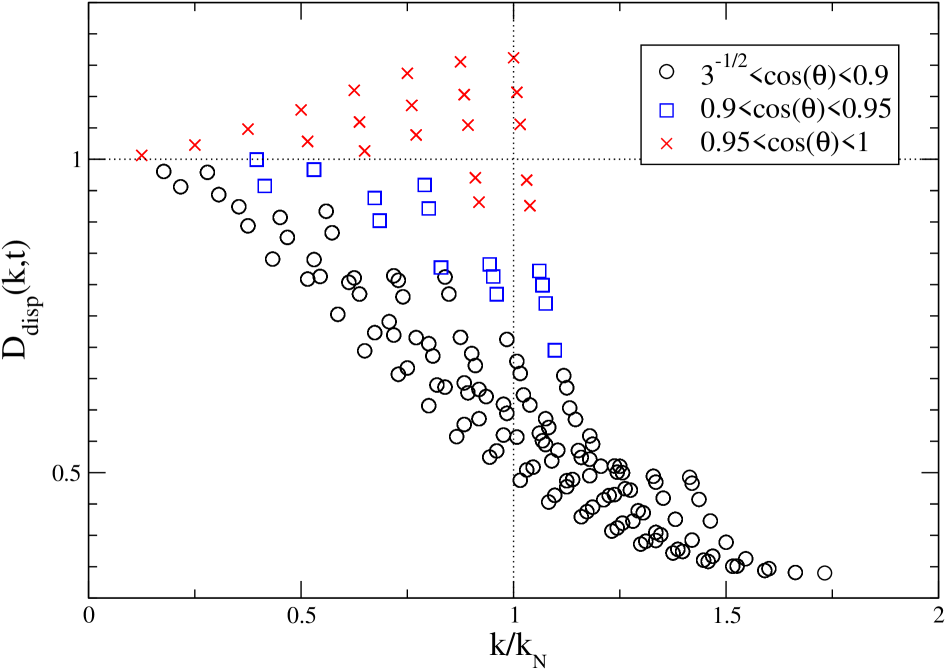
Figure 2: Discreteness factor $D_{\rm disp}({\bf k},t)$ quantifying the modification with respect to the fluid limit ($D_{\rm disp}({\bf k},t)=1$) of the power in the mode ${\bf k}$ of the evolved displacement field. The plot is given at at $a=5$ (for a simulation starting at $a=1$). See text for further details.

In Fig. 2 is shown $D_{\rm disp}({\bf k},t)$ for the value $a=5$, i.e., after evolution from IC set at $a=1$. Deviations from unity are a direct measure of the modification of the theoretical (fluid) evolution introduced by the discreteness up to this time. Note that $D_{\rm disp}({\bf k},t)$ is plotted as a function of $k$, each point corresponding to a different value of ${\bf k}$. The fact that the evolution depends on the orientation of the vector ${\bf k}$ is a manifestation of the breaking of rotational invariance by the lattice discretisation. The three different symbols for the points correspond to three different intervals of the cosine of the minimum angle $\theta$ between the vector ${\bf k}$ and one of the axes of the lattice. We will return to this point in further detail below.

We have chosen the value $a=5$ because it is of the order of the typical one at which shell crossing occurs in $N$-body simulations, i.e., the initial amplitude in these simulations is typically such that this is the case. As we have already noted, the discrete evolution and the fluid one are described by different exponents, so this figure of $D_{\rm disp}({\bf k},a)$ will change as we change $a$. The resemblance between Fig. 2 and the optical branch of the dispersion relation in Fig. 1 allows us to infer simply this evolution: the reason for this resemblance is that already at the time chosen ($a=5$), the expression (34) is well approximated by the regime $t\gg t_{0}$, given by Eq. (28), in which the most rapidly growing eigenmodes, which are those on the optical branches, dominate. Using Eq. (28) it is easy to verify that

$$D_{\rm disp}({\bf k},t\gg t_{0})\approx$$

$$\left[\frac{{(\bf\hat{k}}\cdot{\bf{\hat{e}}}_{\rm max}({\bf k}))(2+3\alpha_{\rm max}^{+}({\bf k}))}{3(\alpha^{-}_{\rm max}({\bf k})+\alpha^{+}_{\rm max}({\bf k}))}\right]^{2}\left(\frac{t}{t_{0}}\right)^{2[\alpha^{-}_{\rm max}({\bf k})-\frac{2}{3}]}\,.$$ (36)

For small $k$ (compared to $k_{N}$) we can simplify this expression. In this case Marcos et al. (2006) the eigenvalues on the optical branch can be treated in a Taylor expansion about the fluid limit:

$$\epsilon({\bf k})\approx(1-b({{\bf\hat{k}}})k^{2}\ell^{2})\,,$$ (37)

where $b({\bf\hat{k}})$ is a dimensionless coefficient of order unity which depends on the direction in reciprocal space. This expression is in fact Marcos et al. (2006), for the simple cubic lattice, a good approximation to the eigenvalues up to $k\approx k_{N}$. Using it we have

$$D_{\rm disp}({\bf k},a) \approx \left(1+\frac{12}{25}b(\hat{\bf k})\ell^{2}k^{2}\right)$$ (38)

$$\times ({\bf\hat{k}}\cdot{\bf{\hat{e}}}_{\rm max}({\bf k}))^{2}a^{-\frac{6}{5}b(\hat{{\bf k}})k^{2}\ell^{2}}$$

and therefore

$$D_{\rm disp}({\bf k},a\gg 1)\approx({\bf\hat{k}}\cdot{\bf{\hat{e}}}_{\rm max}({\bf k}))^{2}\cdot a^{-\frac{6}{5}b(\hat{{\bf k}})k^{2}\ell^{2}}\,.$$ (39)

In Fig. 3 is shown $D_{\rm disp}({\bf k},a)$, now averaged over all ${\bf k}$ in a narrow bin of $k$, for different values of $a$. As anticipated we see that the discreteness effects, i.e., the deviation from unity of this quantity, grows as a function of time. Also shown are the corresponding averages of the approximate expression Eq. (38) . We see that the agreement is very good, as expected, for sufficiently small $k$ and $a$.

Figure 3: Discreteness factor $D_{\rm disp}({\bf k},t)$ for $a=2$, $a=5$ and $a=10$, averaged over bins of $\Delta|{\bf k}|=0.03k_{N}$ for a $64^{3}$ simple cubic lattice. In each case is plotted also the equivalent average of the analytic approximation given in Eq. (38).

III.2 The power spectrum of density fluctuations

We have considered above the evolution of the two point properties of the displacement fields. Usually in the cosmological context one is more interested in a direct characterization of the evolution of the density fluctuations, notably through the power spectrum of density fluctuations or its Fourier transform, the reduced two-point (density-density) correlation function. In the cosmological literature the relation between the two quantities is invariably derived in the continuous limit (see e.g. Schneider and Bartelmann (1995)). Instead we use here the more general result derived in Gabrielli (2004), which gives the PS of density fluctuations of a discrete distribution of points generated by applying a generic stochastic displacement field with two point correlation matrix $S_{\mu\nu}({\bf r})$ to a distribution with initial PS of density fluctuations $P_{in}({\bf k})$:

$$P({\bf k}) = \int d^{3}re^{-i{\bf k}\cdot{\bf r}}e^{-k_{\mu}k_{\nu}[S_{\mu\nu}(0)-S_{\mu\nu}({\bf r})]}\left(1+\tilde{\xi}_{in}({\bf r})\right)$$ (40)

$$- (2\pi)^{d}\delta({\bf k}),$$

where $\tilde{\xi}_{in}({\bf r})$ is the Fourier transform of $P_{\rm in}({\bf k})$, i.e., the reduced two point correlation function of the initial distribution, and the integral is over all space (as the expression applies in the infinite volume limit, i.e., to an infinite point distribution).

Expanding the exponential factor $e^{-k_{\mu}k_{\nu}[S_{\mu\nu}(0)-S_{\mu\nu}({\bf r})]}$ to linear order one obtains

$$P({\bf k}) = P_{in}({\bf k})+k_{\mu}k_{\nu}S_{\mu\nu}({\bf k})$$

$$+ \frac{k_{\mu}k_{\nu}}{(2\pi)^{3}}\int d^{3}qS_{\mu\nu}({\mathbf{q}})[P_{in}({\bf k}+{\mathbf{q}})-P_{in}({\bf k})]\,.$$

Note that in reciprocal space we now have an integral, rather than a sum, as the density field is defined everywhere in real space. For the case we are studying here, however, of a lattice with finite periodicity, the displacement field inherits the same periodicity and thus the function $S_{\mu\nu}({\bf k})$ is non-zero only on the reciprocal lattice. The integral therefore reduces again to a sum.

In Joyce and Marcos (2007) we have studied in detail the domain of validity of this linearized approximation Eq. (III.2) to the full expression Eq. (40). This depends in general on the shape of the input PS $P_{th}(k)$, but for the PS in the range typical of cosmological models the criterion is just that the variance of the relative displacement of particles be small compared to the distance separating them. This coincides precisely with the range of validity of PLT. Using then Eq. (III.2) with the PS of the displacements as given by Eq. (31), we obtain

$$P({\bf k},t)=P_{in}({\bf k})+({\bf\hat{k}}\cdot{\bf E}({\bf k},t))^{2}P_{\rm th}(k)$$ (42)

$$+\frac{k^{2}}{(2\pi)^{3}}\int d^{3}q({\bf\hat{k}}\cdot{\bf E}({\mathbf{q}},t))^{2}\frac{P_{\rm th}(q)}{q^{2}}[P_{in}({\bf k}+{\mathbf{q}})-P_{in}({\bf k})]$$

where we have used the Poisson equation with Eqs. (19) to relate the input theoretical PS $P_{th}(k)$ to the applied displacement fields through

$$k^{2}|{\tilde{u}}({\bf k},t_{0})|^{2}=P_{\rm th}(k,t_{0})\,.$$ (43)

Eq. (42) is thus the expression for the evolved PS of the density fluctuations in and $N$-body simulation (on a perturbed lattice) as given by PLT. The effects of discreteness described may be divided into two:

• Effects encoded in the dependence of the function ${\bf E}({\bf k},t)$ on the lattice spacing $\ell$, which give as we have discussed deviations from its fluid value ${\bf\hat{k}}a(t)$. This is manifestly a dynamical effect of discretization on the lattice.

• Effects encoded in the additional dependence on the lattice spacing $\ell$ of the first and third term on the right hand side of Eq. (42). This dependence comes through the initial PS $P_{in}({\bf k})$. These terms describe the density fluctuations which are associated to the discrete sampling of the PS given by the second term on the right hand side of Eq. (42), on the lattice. They thus correspond to a static effect of the discretization.

The first term on the right hand side of Eq. (42) depends only on the second effect — and is thus independent of time, describing simply the static contribution of the initial unperturbed lattice — while the second term depends only on the first effect. The third term, however, couples both effects. It describes, as we shall see, how purely discrete power, at large $k$ is induced and evolves in time.

$P_{in}({\bf k})$, which is the PS of the lattice, is simply proportional to an infinite sum of delta functions at all points of the reciprocal lattice, i.e., at ${\bf k}=2k_{N}{\bf m}$ where ${\bf m}$ is any vector of non-zero integers. This term thus vanishes in the first Brillouin zone [as defined after Eq. (12) above]. It is straightforward to show Joyce and Marcos (2007) that the same is true for the third (convolution) term in Eq. (42), provided the input PS is appropriately set equal to zero outside the first Brillouin zone. The second term on the right hand side of Eq. (42) is thus the only term which is non-zero inside the first Brillouin zone. The non-trivial discreteness effects described by the second and third terms on the right hand side of Eq. (42) thus contribute in non-overlapping regions of reciprocal space.

III.2.1 PS inside first Brillouin zone

As we have just seen the evolved PS inside the first Brillouin zone, to linear order in the input PS, is

$$P({\bf k},t)=({\bf\hat{k}}\cdot{\bf E}({\bf k},t))^{2}P_{\rm th}(k)\,.$$ (44)

To characterize the effects of discreteness we thus define

$$D_{\delta\rho}({\bf k},t) \equiv \frac{P({\bf k},t)}{P^{\rm fluid}(k,t)}$$ (45)

$$= \frac{|{\bf\hat{k}}\cdot{\bf E}({\bf k},t)|^{2}}{|{\bf\hat{k}}\cdot{\bf E}^{\rm fluid}({\bf\hat{k}},t)|^{2}}$$

$$= \frac{|{\bf\hat{k}}\cdot{\bf E}({\bf k},t)|^{2}}{a^{2}(t)}\,,$$

where, using the definitions given above, we have

$$|{\bf\hat{k}}\cdot{\bf E}({\bf k},t)|^{2}=\left[\sum_{n=1}^{3}[U_{n}({\bf k},t)+\frac{2}{3t_{0}}V_{n}({\bf k},t)](\hat{\mathbf{e}}_{n}\cdot\hat{\bf k})^{2}\right]^{2}$$ (46)

instead of the expression in Eq. (34) for the analogous quantity for the PS of the displacement fields.

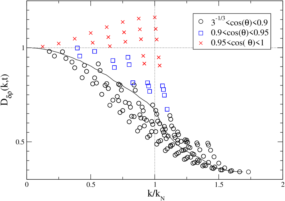
Figure 4: Discreteness factor $D_{\delta\rho}({\bf k},t)$ quantifying the modification with respect to the fluid limit ($D_{\delta\rho}({\bf k},t)=1$) of the power in the mode ${\bf k}$ of the evolved density fluctuation field, for ${\bf k}$ in the FBZ. The plot is given, as for Fig. 2, at $a=5$ (for a simulation starting at $a=1$), for a $16^{3}$ simple cubic lattice. Also shown is a curve corresponding to the same quantity averaged over all ${\bf k}$ with $k$ in one of bins of equal width $\Delta k=0.03k_{N}$, for a $64^{3}$ simple cubic lattice. (The points of this $64^{3}$ calculation, which are not shown, just trace more densely the behaviour of the points shown.)

In Fig. 4 is shown $D_{\delta\rho}({\bf k},t)$, at $a=5$ as for the analogous Fig. 2 for the displacement fields in the previous subsection. The two figures are in fact very similar, particularly at smaller $k$. The reason is the same one which explained the similarity between Fig. 2 and the optical branch of Fig. 1: the most rapidly growing mode on this branch already dominates at this time so that the difference between the expression in Eqs. (34) and (46) reduces to a trivial time independent factor. Indeed we have now

$$D_{\rm\delta\rho}({\bf k},t\gg t_{0})\approx{(\bf\hat{k}}\cdot{\bf{\hat{e}}}_{\rm max}({\bf k}))^{4}$$ (47)

$$\times\left[\frac{(2+3\alpha_{\rm max}^{+}({\bf k}))}{3(\alpha^{-}_{\rm max}({\bf k})+\alpha^{+}_{\rm max}({\bf k}))}\right]^{2}\left(\frac{t}{t_{0}}\right)^{2[\alpha^{-}_{\rm max}({\bf k})-\frac{2}{3}]},$$

which differs from Eqs. (36) only by the power of the product ${\bf\hat{k}}\cdot{\bf\hat{e}}_{\rm max}({\bf k})$. We do not plot the analogous curves to those of Fig. 3 as the results look essentially the same.

At $a=5$ (i.e. at the time of shell crossing in a typical cosmological $N$-body simulation) our Fig. 4 is a plot of the fractional discrepancy between the theoretically evolved power (by FLT) and the power as evolved in the discretization of this system (by PLT). The fractional error introduced by the discretization is largest, unsurprisingly, for the modes at the very largest wavenumbers ($k=\sqrt{3}k_{N}$, at the extremities of the first Brillouin zone), and decreases as $k$ does. At $a=5$ the power in the largest mode is reduced to about one third of its fluid value, while around $k=k_{N}$ the fractional error varies from about $+10\%$ to more than $-50\%$. At $k=k_{N}/2$ it varies from $+5\%$ to about $-20\%$, while at $k=k_{N}/4$ the total spread is about $10\%$.

In Fig. 4 is shown also an average of $D_{\delta\rho}({\bf k},a)$ (at $a=5$) over narrow bins of equal width in $k$, for a larger $64^{3}$ lattice. We see that this average is dominated, at this time, by the more numerous modes with growth coefficients which are smaller than the fluid one. We see that this average describes at all $k$ a net slowing down of the evolution of the power in the density fluctuations, ranging from slightly more than $30\%$ at the Nyquist frequency, to $10\%$ at half this frequency, and down to about $3-4\%$ at one quarter. It is straightforward to refine these estimates given the precise parameters of a simulation (i.e. the initial amplitudes to determine time of shell-crossing). In our conclusions we will discuss the importance of these effects, and how they might be corrected for in simulations.

III.2.2 PS outside the first Brillouin zone

For ${\bf k}$ outside the FBZ, we have in Eq. (42) only the non-trivial contribution from the third term. Taking an input theoretical PS of the form

$$P_{th}(k)=Ak^{n}f(k/k_{c})\,$$ (48)

where $f(k/k_{c})$ is a function which cuts off the PS at $k>k_{c}$, it is straightforward to show (see Joyce and Marcos (2007) for further detail) that this term can be written

$$P_{\rm d}^{(1)}(k)=Ak^{2}k_{N}^{n-2}I(\mathbf{k})$$ (49)

where

$$I(\mathbf{k})=\sum_{\mathbf{h}\neq\mathbf{0}}[\mathbf{\hat{k}}\cdot{\bf E}(\mathbf{h}-\mathbf{k},t)]^{2}\left(\frac{|\mathbf{h}-\mathbf{k}|}{k_{N}}\right)^{n-2}$$

$$\times f\left(\frac{|\mathbf{h}-\mathbf{k}|}{k_{c}}\right)\Theta_{FBZ}(\mathbf{h}-\mathbf{k})$$ (50)

where $\mathbf{h}=2k_{N}{\bf m}$, and the sum runs over all integer vectors ${\bf m}$, and $\Theta_{FBZ}(\mathbf{h}-\mathbf{k})$ is a three dimensional Heaviside function which is equal to unity inside the first Brillouin zone, and zero elsewhere. This cut-off is imposed, as discussed above, in order to avoid aliasing effects.

At a given ${\bf k}$ the sum $I(\mathbf{k})$ can pick up contributions only from a single vector $\mathbf{h}$, the one which lies inside the FBZ when translated by $-{\bf k}$. It thus has the intrinsic periodicity of the lattice PS itself, i.e., $I(\mathbf{k})=I(\mathbf{k}+\mathbf{h})$, and it thus suffices to calculate it for vectors ${\bf k}$ such that $k_{N}\leq k_{i}<2k_{N}$. Just outside the FBZ it picks up contributions from ${\bf h}$ such that $\mathbf{h}-\mathbf{k}$ lies just inside the FBZ, and thus of order $f(k_{N}/k_{c})$, while at the larger values $k\sim 2k_{N}$ it picks up contributions from ${\bf h}$ such that $\mathbf{h}-\mathbf{k}\rightarrow 0$, with an amplitude which depends strongly on the exponent $n$ of the input power spectrum. For any $n<2$, as is always the case in cosmological models, the amplitude diverges as one approaches ${\bf k}=2k_{n}{\bf m}$ (where $P_{in}(k)$ is also divergent).

The term in the PS given in Eq. (49) thus describes how the power at all wavenumbers in the input PS gives rise to power at small scales. Like the power $P_{in}({\bf k})$ associated with the unperturbed lattice, it is purely discrete. Differently from this latter term, which is time independent, it evolves in time as described by PLT. It thus describes evolving physical clustering in the simulations which is entirely an artifact of discreteness, rather than, as in the effects analyzed above, a modification due to discreteness of the non-trivial clustering of the fluid limit. Indeed it is interesting to note that, even if we take $k_{c}<<k_{N}$, i.e., a cut-off in the input PS (as for example in typical in hot or warm dark matter simulations), this term is non-zero, and the growth can be well approximated by using the fluid limit for ${\bf E}({\bf k},t)$ (since for the terms contributing in the sum $|\mathbf{h}-\mathbf{k}|\ell\ll 1$). We will discuss this term further in our conclusions below.

III.3 Measures of anisotropy

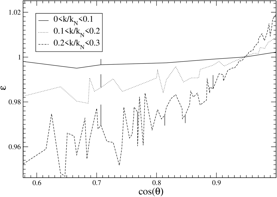
Figure 5: Average value $\varepsilon$ of the normalized eigenvalues $\epsilon_{n}({\bf k})=-\omega_{n}^{2}({\bf k})/4\pi G\rho_{0}$, averaged over the maximal eigenvalues at each ${\bf k}$ for $k$ in the different ranges indicated, as a function of $\cos\theta$, the minimal angle between ${\bf k}$ and any axis of the lattice.

Let us consider in more detail the effects of anisotropy in the evolution induced by the lattice discretization. The different symbols indicated in Fig. 2 and Fig. 4 correspond, as has been noted, to the different ranges of the cosine of the minimum angle $\theta$ between the vector ${\bf k}$ and one of the lattice directions. This is, of course, just a direct result of the dependence of the eigenvalues on this quantity evident in Fig. 1, which is a manifestation of the anisotropy of the lattice. In Fig. 5 we plot the eigenvalue as a function of $\cos\theta$ for the maximal eigenvalue (i.e. on the optical branch) averaged over different ranges of $k$. The degree of anisotropy over the range of orientations is roughly characterized by the slope of these curves (as zero slope corresponds to isotropy). We see clearly that the amplitude of the anisotropy thus decreases as the typical $k$ in the chosen bin decreases, which is as expected as we approach the fluid limit [for which $\varepsilon=1$]. We observe also a clear trend in the deviation from the fluid eigenvalue: this deviation typically increases as the orientation of the corresponding eigenvector goes further away from the axes of the lattice. This behaviour is, however, not exactly followed, in particular around $\cos\theta=1$ . Indeed it is notable that the eigenmodes oriented parallel, or very close to parallel, to the lattice planes have eigenvalues which are larger than the fluid one. We note that the very largest eigenvalue in Fig. 1, associated with the largest values of $D_{\rm disp}$ and $D_{\delta\rho}$ in Figs. 2 and 4, correspond to an exactly longitudinal mode with $k=k_{N}$ and ${\bf k}$ parallel to the axes of the lattice. It thus describes the motion of pairs of adjacent infinite planes towards one another. The eigenvalue of this mode (see Fig. 1) is $\epsilon\approx 1.1$, which gives [using Eqs. (III.2.1) and (67)] $D_{\delta\rho}\propto a^{0.12}$.

There are clearly many different ways of quantifying these effects. One simple measure is the dispersion in the growth of the power in modes of the displacement or density fields. Considering the latter we define

$$\Delta D_{\delta\rho}(k,t) = \left(\frac{\overline{D_{\delta\rho}^{2}}(k,t)-\overline{D_{\delta\rho}}^{2}(k,t)}{\overline{D_{\delta\rho}}^{2}(k,t)}\right)^{1/2}$$

$$= \left[\overline{\left(\frac{|{\bf\hat{k}}\cdot{\bf E}({\bf k},t)|^{2}-{\overline{|{\bf\hat{k}}\cdot{\bf E}({\bf k},t)|^{2}}}}{{\overline{|{\bf\hat{k}}\cdot{\bf E}({\bf k},t)|^{2}}}}\right)^{2}}\right]^{1/2}\,,$$

where the second equality is valid in the FBZ. The average, of any function ${X}({\bf k},t)$ on the reciprocal lattice, is defined as

$$\overline{X}(k,t)=\frac{1}{N_{k}}\sum_{{\bf k},|{\bf k}|=k}{X}({\bf k},t)\,,$$ (52)

$N_{k}$ being the number of eigenmodes at a given $k$. $\Delta D_{\delta\rho}(k,t)$ is evidently defined so that it is zero in the absence of anisotropy, and in particular in the fluid limit. Its value, averaged in narrow bins of $k$, is plotted in Fig. 6, for three different times corresponding to the scale-factors $a$ indicated (where, as before, $a=1$ corresponds to the beginning of the simulation). The results are very much as one would anticipate from Fig. 4: the anisotropy is greatest around $k=k_{N}$ where the spread in the growth factors is greatest, and the amplitude at any $k$ grows as a function of $a$. Note that for a typical $N$-body simulation, with $a=5$ at shell crossing, the dispersion in the growth factor at this time at $k=k_{N}$ is of order $20\%$.

Figure 6: Discreteness factor $\Delta D_{\delta\rho}(k,t)$ for $a=2$, $a=5$ and $a=10$, averaged over bins of $\Delta|{\bf k}|=0.03k_{N}$ for a $N=64^{3}$ simple cubic lattice.

One simple manifestation of the anisotropy introduced in the evolution by the discretisation on a lattice was noted by Melott et al. in Melott et al. (1997) : an initial perturbation described by a pure plane wave, which in the fluid limit should maintain its purely one dimensional character, can become three dimensional. The breaking of symmetry associated is, up to numerical precision, entirely associated to the lattice. In Melott et al. (1997) the authors studied this effect numerically, notably as function of the smoothing at small scales. One simple quantitative characterization of this effect is

$${D}_{\rm aniso}({\bf k},t)=\frac{|\bf{\tilde{u}}({\bf k},t)-{\bf\hat{k}}[{\bf\hat{k}}\cdot\bf{\tilde{u}}({\bf k},t)]|^{2}}{|{\bf\hat{k}}\cdot\bf{\tilde{u}}({\bf k},t)|^{2}},$$ (53)

i.e., the fractional deviation of the displacement direction parallel to ${\bf k}$. It follows from Eq. (23) that

$${D}_{\rm aniso}({\bf k},t)=\frac{{\bf E}^{2}({\bf k},t)}{({\bf\hat{k}}\cdot{\bf E}({\bf k},t))^{2}}\,,$$ (54)

which is evidently unity in the fluid limit. For $t\gg t_{0}$ it follows, from Eqs. (36) and (III.2.1), that

$${D}_{\rm aniso}({\bf k},t\gg t_{0})=\frac{1}{({\bf\hat{k}}\cdot{\bf e}_{\rm max}({\bf k}))^{2}}\,,$$ (55)

i.e., it is independent of time, depending only on the orientation of the eigenvector of the maximally growing mode with respect to ${\bf k}$. This quantity, averaged over narrow bins of $k$, is shown in Fig. 7. We see the convergence to the fluid limit, in which ${\bf\hat{e}}_{\rm max}({\bf k})\rightarrow{\bf\hat{k}}$, for $k/k_{N}\ll 1$ and increasing deviations as $k$ increases.

Figure 7: The asymptotic time independent anisotropy factor $D_{\rm aniso}(k,t>>t_{0})$ defined in the text averaged over bins of $\Delta|{\bf k}|=0.03k_{N}$, for a $64^{3}$ simple cubic lattice.

IV Discreteness effects with a small scale smoothing

In cosmological $N$-body simulations a smoothing at small scales of the interparticle (Newtonian) potential is generally employed Efstathiou et al. (1985); Couchman (1991). “Small” in this context means that the characteristic scale for this modification of the potential is smaller or comparable to the average initial inter-particle distance, i.e., approximately the lattice spacing $\ell$ in the case we are considering, of perturbations from a lattice. Almost always in fact this smoothing is taken to be considerably (i.e. one to two orders of magnitude) smaller than $\ell$; an exception is in $PM$ simulations in which the effective smoothing scale is normally equal to the scale $\ell$, as the potential is calculated on a mesh which typically is taken to coincide with the initial lattice configuration. There is in this case no correction to take into account forces from sub-mesh particles, as in $P^{3}M$ or tree codes (see e.g. Efstathiou et al. (1985); Couchman (1991)).

The motivation for the use of such a smoothing in this context is that it should reduce the effects of discreteness and make the simulation approximate better the theoretical (fluid-like) behaviour. The reason for this expectation is that it reduces the impact of hard two-body collisions, which should be negligible in the fluid limit (in which the mean-field dominates). However, there is no demonstration (more than these approximate qualitative arguments) that such a smoothing has the effect of making a simulation a better approximation to the desired fluid limit. Indeed attempts in the literature to treat this question numerically (e.g. Splinter et al. (1998); Kuhlman et al. (1996); Melott (1990); Melott et al. (1997); Diemand et al. (2004a, b); Binney (2004); Hamana et al. (2002)) lead to quite different conclusions. Notably the use of a smoothing smaller than $\ell$ has been contested by some authors Splinter et al. (1998); Kuhlman et al. (1996); Melott (1990); Melott et al. (1997), while such a practice is almost universal in large current $N$-body simulations.

Let us consider what we can learn about this question using the methods developed in this paper. As was noted in Sect. II.1, the perturbative analysis we have described can be applied to any two-body interaction potential, and in particular to the case of a smoothed Newtonian potential. We can simply repeat our calculation of the eigenvalues and eigenmodes given the potential. The form of the smoothing employed varies and has evolved in time. Currently it is common to use a smoothing which leaves an exact $1/r$ potential for $r>\epsilon$, where $\epsilon$ is the scale characteristic of the smoothing. If then $\epsilon\ll\ell$, as is typically the case, this modification has no effect until two particles are closer than $\epsilon$. It therefore has no effect on our calculation (which breaks down when this condition is fulfilled anyway). Thus such a smoothing has no effect in moderating or otherwise the discreteness effects we have quantified. The fact that that this is the case illustrates clearly an important point: the discreteness effects we have described are not two-body collisional effects.

In order for a smoothing of the potential to be of relevance to the effects we are describing it must modify the potential at the interparticle distance, as we do a perturbation expansion about the configuration with the particles at this distance. Let us consider therefore a simple smoothing which does so, the so-called “Plummer” smoothing:

$$\phi(r)=\frac{1}{\sqrt{r^{2}+\epsilon^{2}}}.$$ (56)

When $\epsilon\sim\ell$ it would be expected to, and indeed does, produce results similar to $\mathrm{P}M$ simulations (see e.g. Splinter et al. (1998); Melott (1990))

For a given value of $\epsilon$ we can calculate the spectrum of eigenvalues and eigenmodes. As one would anticipate, the modifications to them with respect to the case of pure gravity, are very small for $\epsilon\ll\ell$, and only becomes significant when we have $\epsilon\sim\ell$. In Fig. 8 we show the eigenvalues on the optical branch, for $\epsilon=\ell/2$. Also plotted, for comparison, is the same branch for pure gravity.

The conclusions which follow from this figure are very clear. The effects of introducing a significant smoothing is to increase the average amplitude of discreteness effects, while decreasing the effects of anisotropy. These behaviours are straightforward to understand qualitatively. The contribution to the total gravitational forces coming from nearby particles starts to be reduced significantly when the smoothing becomes of order the interparticle distance. Thus the growth factors at these scales decrease relative to the case of full gravity, but they also show less anisotropy as the strong anisotropy in the distribution of nearest neighbors is no longer felt as much.

Figure 8: Eigenvalues of the eigenmodes of the displacement fields for full gravity (top set), and with a smoothing at half the interparticle distance (see text), for a $64^{3}$ simple cubic lattice. For clarity only $0.5\%$ of the eigenvalues are shown for $k/k_{N}>0.2$.

These effects can easily be further quantified by considering the effects of varying the smoothing scale $\epsilon$ on the quantities we defined above. In Fig. 9 we show the fluid-normalized discreteness factor $D_{\rm disp}$ [as defined in Eq. 45] both without any smoothing (as in Fig. 3) and for $\epsilon=\ell/2.$ The result is self-evident given the results for the optical branch in Fig. 8 above: the smoothing increases the effects of discreteness on average. The expected reduction in anisotropy as $\epsilon$ increases is illustrated in Fig. 10, which shows the asymptotic value of the function ${D}_{\rm aniso}$ [as defined in Eq. 53] for three values of $\epsilon$. As the latter parameter increases, we see that on average the optical modes become more longitudinal which results in a reduced symmetry breaking effect in the propagation of plane waves. This is indeed the conclusion of the numerical study of this discreteness effect in Melott et al. (1997). We note, however, that the present analysis leads to a conclusion different to that of Melott et al. (1997): while the smoothing reduces this effect of discreteness, it actually increases the averaged effect of discreteness. By increasing the smoothing scale one obtains a better approximation to fluid behaviour only in the limited sense that one recovers better one qualitative feature of fluid behaviour, its isotropy.

Figure 9: Discreteness factor $D_{\rm disp}({\bf k},t)$ for two different values of the smoothing parameter $\epsilon$ (in units of $\ell$), for $a=2$ and $a=10$ for a $64^{3}$ simple cubic lattice. An average over bins of width $\Delta|{\bf k}|=0.03k_{N}$ has been performed.

Figure 10: The asymptotic anisotropy factor $D_{\rm aniso}(k,t\gg t_{0})$ averaged over bins of $\Delta|{\bf k}|=0.03k_{N}$, for three values of the smoothing parameter $\epsilon$, for a $64^{3}$ simple cubic lattice.

V Parametric and limiting behaviours

We have given in the precedent sections various measures of the modification of the fluid limit evolution engendered by discretization on a lattice. We have made use throughout of the result of Joyce et al. (2005); Marcos et al. (2006), which we have summarized in Sect. II.2, that the fluid limit for the evolution of a given mode is recovered exactly when we send $\ell\rightarrow 0$ while keeping $k$ fixed. We have also seen that, keeping $\ell$ fixed, the deviations of the evolution of this same mode from its fluid behaviour at shell crossing increases as the time of shell crossing does. This implies that the evolution of cosmological simulations deviates completely from the desired theoretical evolution in the limit that the starting red-shift is increased keeping all other parameters fixed. Given these subtleties about how the continuous limit is recovered, it is instructive to consider these points in greater detail.

V.1 The fluid limit

Let us consider carefully in what limit the desired fluid limit for the evolution of a cosmological $N$-body simulation (in the class considered here) is recovered.

Such a simulation, periodic on a cube of side $L$, is a discretisation of the continuum problem, which introduces, at least, the following parameters:

• the lattice spacing $\ell$, given by $\ell=L/N^{1/3}$,

• the force smoothing scale $\epsilon$, and

• the initial red-shift $z_{\rm init}$.

The interpretation of results of the simulation as physical is justified if they approximate well those which would be obtained by simulations with suitable extrapolations of these parameters towards the theoretical continuum limit. The importance of understanding this limit precisely is that it explains how this extrapolation of the parameters should be performed in practice.

The input theoretical cosmological model, on the other hand, is characterized fully, for Gaussian initial fluctuations, by its PS. If the side $L$ of the box is specified in physical units, the applicability of the ZA for setting up the IC then fixes, for given $\ell$, a minimal value of the initial red-shift $z_{\rm init}$. This corresponds to an upper bound on the initial amplitude of the PS. The PS is, in general, a function which involves numerous physical scales characteristic of the cosmological model. It contains necessarily, however, at least one such scale: that characterising decay at large $k$ of the PS. Indeed since the one point variance of the density fluctuations, which is proportional to the integral of the PS, is necessarily finite, one has that

$$\lim_{k\rightarrow\infty}k^{3}P(k)=0\,.$$ (57)

There is thus always a physical scale given by a wavenumber $k_{c}$, above which fluctuations of density decay faster than $k^{-3}$. In simulations of the currently favored cold dark matter (CDM) models $\ell$ is always, because of numerical limitations, much larger than $k_{c}^{-1}$ (i.e. $k_{c}$ is larger than the particle Nyquist frequency), and the displacement field generated is then cut-off in the first Brillouin zone rather than at $k_{c}$ (to avoid aliasing effects). In hot or warm dark matter (HDM or WDM) models, on the other hand, the (approximately exponential) cut-off is typically at a wavenumber considerably smaller than the Nyquist frequency.

The exact fluid limit, in the regime of application of PLT, is that in which the corrections due to discreteness vanish, i.e., all the terms in Eq. (29) vanish exactly and the particles follow the exact FLT trajectories. It is clear that, strictly, this occurs only if we impose an abrupt cut-off $k_{c}$ in the input spectrum of modes, which remains fixed as the particle number increases, i.e., the exact fluid limit is $k_{c}\ell\rightarrow 0$ at fixed $k_{c}$. We can, in practice, identify this $k_{c}$ with the (not necessarily abrupt) cut-off in the input PS: modes for $k>k_{c}$ do not contribute significantly to the usually physical relevant quantities (such as mass variance).

To specify fully the limit we need to prescribe how the other parameters, $z_{\rm init}$ and $\epsilon$, are treated. It is clear that it is sufficient to keep $z_{\rm init}$ fixed for what has been said above to hold. As for $\epsilon$, we have seen that it leads to a modification of the growth of modes with respect to their fluid evolution, so the latter will only be recovered if $\epsilon\rightarrow 0$ as $\ell\rightarrow 0$, i.e., $\epsilon\rightarrow 0$ in physical units. Given that PLT is well defined for $\epsilon=0$ the order in which one takes the two limits is clearly not important.

V.2 Long time/high initial red-shift limit

We have seen that, because the modification of evolution associated to discreteness appears as a difference in the exponents of growth of any given mode, the discrete system, with a given $\ell$, diverges from the fluid one when one considers the long time limit for any given $k$ if $\ell$ remains fixed. Indeed for $k<k_{N}$ we have seen, for example, that the statistical measures of discreteness effects in the evolution of the PS of density fluctuations $D_{\delta\rho}$ is well approximated by Eq. (III.2.1). This expression diverges at large times arbitrarily far from the fluid limit, $D_{\delta\rho}=1$. These PLT approximations remain good until close to shell crossing at the scale $\ell$ which occurs at a red-shift determined by the cosmological model (and independent of the choice of the initial red-shift $z_{\rm init}$ for the simulation). Thus, for a given physical scale, discreteness effects increase without limit as the starting red-shift of the simulation is increased, at fixed particle number. For asymptotically large values any physical quantity will be dominated by the modes with the largest exponents. In the case of the simple cubic lattice, as we have noted above, these modes correspond to the collapse of infinite planes along the axes of the lattice.

It follows from this discussion that, in the fluid limit we defined above, the order of the limits for $N$ (or $\ell$) and for the duration $t$ of the simulation (or $z_{\rm init}$), is important, i.e.,

$$\lim_{z_{\rm init}\rightarrow\infty}\lim_{\ell\rightarrow 0}\neq\lim_{\ell\rightarrow 0}\lim_{z_{\rm init}\rightarrow\infty}\,,$$ (58)

or, equivalently,

$$\lim_{t\rightarrow\infty}\lim_{N\rightarrow\infty}\neq\lim_{N\rightarrow\infty}\lim_{t\rightarrow\infty}\,.$$ (59)

This result is in fact not surprising, at least for those familiar with the use of the Vlasov limit to describe systems (e.g. plasmas) with long range interactions. It is in fact well known (e.g. Braun and Hepp (1977); Spohn (1991)) that there is a non-commutativity of the long time and large number limits in such systems. The Vlasov limit corresponds to taking the particle number to infinity before the time. The long time limit of a system with fixed $N$ is a different physical limit of the system’s behaviour. Indeed a good example of this are precisely the two-body collisional effects usually considered as sources of discreteness error in $N$-body simulation: these become relevant Binney and Tremaine (1994), in a uniform system with mean density $\rho_{0}$ on a time-scale $t_{2}\sim t_{dyn}N/\ln N$ where $t_{dyn}=1/\sqrt{4\pi G\rho_{0}}$. Thus clearly if one considers the limit $t\rightarrow\infty$ at finite $N$ one never recovers the Vlasov behaviour. Toy models in one dimension manifesting this kind of behaviour have recently been studied in detail (see e.g. Yamaguchi et al. (2004)).

Practically this observation implies that at least one of the conditions for keeping discreteness effects under control in an $N$-body simulation is a constraint on the initial red-shift (i.e. given $\ell$, that $z_{\rm init}$ be less than some value). We note that the $z_{\rm init}$ is not a parameter which has been considered in discussions of discreteness effects in $N$-body simulations in the literature (e.g. Melott et al. (1997); Splinter et al. (1998); Melott (1990); Kuhlman et al. (1996); Hamana et al. (2002)).

V.3 $N$ dependence of effects

It is instructive also to consider more explicitly the $N$ dependence of the effects we have described. A characteristic time scale for these effects, somewhat analogous to the one just refered to for two-body relaxation, can be derived by considering the evolution we have described here in static space (i.e. with $a(t)=1$). The only modification with respect to the EdS case we have treated here is in the mode functions, which become simply growing and decaying exponentials. Fluctuations on all but the shortest scales have eigenvalues which may be well approximated by Eq. (37), or

$$\omega({\bf k})\simeq[1-\frac{b({{\bf\hat{k}}})}{2}k^{2}\ell^{2})]t_{dyn}^{-1}$$ (60)

where $\omega({\bf k})=t_{dyn}^{-1}$ is the fluid behaviour [and $b({{\bf\hat{k}}})$ is a constant of order unity]. For any quantity dominated by modes around ${\bf k}$ the deviation from fluid behaviour will become significant when

$$e^{b({{\bf\hat{k}}})k^{2}\ell^{2}t/2t_{dyn}}\sim 1\,.$$ (61)

The characteristic time scale for the discreteness effects to dominate may thus be estimated as

$$t_{disc}(k)\sim\frac{t_{dyn}}{k^{2}\ell^{2}}\propto N^{2/3}$$ (62)

where the last proportionality is inferred for a given $k$ (fixed in units of the box size as the particle number $N$ increases). Note that here $N$ is the number of particles sampling the scale $\sim k^{-1}$ rather than the total number of particles in the system. Thus the time scale for the discreteness effects to dominate is a function of the scale considered rather than a global timescale for the system.

VI Discussion and conclusions

We have described in this paper the application of a formalism developed in Joyce et al. (2005); Marcos et al. (2006) to determine the errors in $N$-body simulations at early times, i.e., up to shell crossing when the formalism breaks down. We have given an explicit expression, Eq. (29), for the error in the trajectory of any particle, assuming only that IC are set up in the standard way using the ZA. We have then defined, evaluated numerically for a typical red-shift of shell-crossing, and given approximate analytic expressions for, functions which characterize these discreteness errors for any given mode of the displacement or density field. We have also discussed the effects of a smoothing of the force at small scale on these effects, as well as the precise limits in which the fluid limit of the system’s evolution is recovered.

We now discuss both the immediate practical relevance of these results — their application in quantitifying a source of systematic error in simulations — as well as their relevance to the broader question of discreteness error in $N$-body simulation, for other kinds of initial configurations and beyond shell crossing.

VI.1 Application of results

We have seen that, at a red-shift of shell crossing typical for a cosmological simulation (with IC using e.g. the code of Bertschinger (1995)), errors larger than a few percent have accumulated for all wavenumbers larger than about a quarter of the Nyquist frequency. Such modes are usually included in the IC in simulations of CDM type models, which typically cut the input PS at the edge of the first Brillouin zone. Indeed this means that for most of the modes included errors are larger : the modes with $k>k_{N}/4$ represent more than $99\%$ of the sampled modes , while those with $k>k_{N}/2$, which have errors exceeding $25\%$, about $93\%$. Any physical quantities at the end of the simulation which depends on the power in these modes must inherit at least this error. Such power is included usually as one is indeed interested in such quantities.

What precisely the induced error is will depend of course on the quantity considered, and we do not attempt here to describe such effects exhaustively. The results given in this paper allow one to calculate them, and thus in principle correct for them, in a very straightforward manner: it suffices to calculate the function $D_{\rm disp}({\bf k},a_{\rm plt})$ as described in Sect. III.1. We have introduced here the scale factor labelled $a_{\rm plt}$ to indicate that up to which PLT is a good approximation. As we have discussed, and shown in detail by numerical study in Marcos et al. (2006), this corresponds approximately to shell crossing. Its precise definition is of course somewhat subjective as it involves specifying how strong a deviation defines it (and in what quantity the deviation is measured). Here it can be taken either as a theoretically calculated shell crossing at the scale $\ell$ or, better, as determined a posteriori from the simulation (e.g. by matching the evolution of the variance of displacements to that described by PLT, as reported in Marcos et al. (2006)).

The effects of discreteness up to shell crossing may thus be considered as equivalent to a ${\bf k}$-dependent misrepresentation of the input displacement field (at $a=1$), by a factor in amplitude of $1/\sqrt{D_{\rm disp}({\bf k},a_{\rm plt})}$. The effective initial amplitude is, for almost all modes, somewhat less than the theoretical amplitude. This could, in principle, be “corrected” for by multiplying each mode ${\bf k}$ of the input displacement field, at the chosen $z_{\rm init}$ (corresponding to $a=1$), by the factor $1/\sqrt{D_{\rm disp}({\bf k},a_{\rm plt})}$. Such a correction would ensure that the full linearized evolution PLT coincides, at $a=a_{\rm plt}$, with the analogous (linearized) fluid result.

It is not clear, however, that such a correction of the initial amplitude will in fact produce a more accurate result than simply starting the simulation at $a=a_{\rm plt}$, using the ZA to set up the IC at this time (and possibly improved taking higher order corrections in Lagrangian perturbation theory into account). Applying the discreteness correction to the IC at $a=1$ ($<a_{\rm plt}$) means that the linear evolution is offset from its theoretical evolution for $a<a_{\rm plt}$. It is possible that the integrated non-linear effect of this offset will be greater than the error involved in using the ZA directly at $a=a_{\rm plt}$ when the linear approximation it is based on is breaking down. In principle there exists a starting red-shift which is optimal in the sense that it minimizes the combined errors due to non-linearity (which decreases as $z_{\rm init}$ increases) and errors due to discreteness (which increases, as we have seen, as $z_{\rm init}$ does). We note in this respect that the perturbative formalism used here, which described the fully discrete problem, can be extended beyond the linear order we have used. Such a treatment should allow a determination of this optimal red-shift.

These comments apply to IC as they are applied in CDM type simulations. In HDM or WDM simulations the physical cut-off in the initial PS is, as has been noted above, typically such that $k_{c}<<k_{N}$. Thus the modes of the displacement field which have the greatest modification of their evolution due to discreteness are not present. For modest typical values of $z_{\rm init}$ the effects just discussed are therefore negligible. Above, however, we discussed only the effects of the modification of the dynamical fluid evolution, and not the additional effects which have been described in Sect. III.2, in the PS of density fluctuations outside the FBZ. We have shown in our discussion of these terms that this additional, purely discrete, contribution in the PS is present even if the input PS is limited to a region well inside the FBZ, as in HDM or WDM simulations. In the approximation that the small $k$ modes grow according to fluid theory (i.e. are linearly amplified in proportion to the scale factor $a$ in the EdS model) it is simply an extra contribution in the initial PS which is also linearly amplified. It describes the growth of power at small scales due to the coupling between long wavelength power and that intrinsic in the initial lattice. We note that this physical mechanism generating “artificial” discrete power at scales of order the initial interparticle distance has been observed and studied in numerical simulations of HDM/WDM Gotz and Sommer-Larsen (2003); Wang and White . Our treatment gives an analytic description of this process (up to shell crossing), for the case of an initial simple cubic lattice.

In this latter context comparative studies have been made of this initial configuration with ones generated starting from the “glass” configurations sometimes used as an alternative White (1993). The formalism we have used in this paper can in principle be generalized to treat such a starting configuration, and thus to compare analytically the discreteness effects up to shell crossing in the different cases. There is, however, a considerable technical complication: the Bloch theorem does not apply and the eigenvectors of the displacement field about the (now approximate) zero force configuration are no longer plane waves. Thus the diagonalization problem cannot be simplified in the same way, and a fully numerical solution would be required to determine the $3N$ eigenmodes. We expect to find only small quantitative differences: the origin of the discreteness effects we have quantified on a lattice arise essentially, as we have discussed just above, from the sampling of the continuous density field by particles. The magnitude of the effects will depend essentially on the average particle density, and not on the details of the arrangement of the points in the distribution.

We note, on the other hand, that the treatment of the problem on other cubic lattices is straightforward. In Marcos the cases of a body-centered cubic and face-centered cubic lattice are solved. We will exploit this treatment of discreteness effects on a range of different “pre-initial” lattices in a forthcoming numerical study of discreteness effects in the non-linear regime Joyce et al. .

VI.2 Discreteness in the non-linear regime

The perturbative treatment presented here can, as has been noted, be extended to beyond linear order. While such an approach may lead to useful insights into the interplay of discreteness effects and non-linearity, it can extend at most as far as shell crossing. The current formalism therefore allows us to say nothing quantitatively about discreteness effects in the fully non-linear regime. It can however, as we now discuss, give us some qualitative insight which may be useful in attempts to understand and quantify such effects.

Discreteness effects, we recall, are all those effects which lead to differences between the evolution of statistical quantities in $N$-body simulations and that in the theoretical Vlasov-Poisson limit. We have underlined that the effects studied here, which are manifestly of this type, are different in nature to those usually emphasized in this context: (i) two-body collisional effects (see e.g Diemand et al. (2004b); Binney (2004); Baertschiger et al. (2002)), and (ii) the limitations imposed by the particle discretisation on the representation of the initial theoretical PS (described analytically in Joyce and Marcos (2007)). The modifications of the continuum evolution we have described here depend explicitly on the dimensionless ratio $k\ell$, and decrease in amplitude as $k\ell$ decreases. They can thus be well described, and distinguished from these other effects, as dynamical sparse sampling effects, i.e., they are modifications of the evolution of fluctuations which arise from the fact that a given scale is sampled more sparsely by the “macro-particles” of an $N$-body simulation than by the microscopic particles of a fluid.

Clearly one would expect that such a physical effect should be present also in the evolution after shell-crossing, in addition to two-body collisional effects and any effects inherited from the IC. The difficulty in assessing its importance, at a given scale and time, is that it is not clear what parameter should play the role of $\ell$ after shell crossing. The results of simulations are usually interpreted as physical down to scales $\sim\epsilon$, where $\epsilon\ll\ell$. This is typically of the order of the interparticle distance in the densest regions of the final configurations (at the centers of halos). This extrapolation would appear then to assume, roughly, that the role of $\ell$ in the non-linear regime is played by the minimal interparticle distance in the evolved simulation. This seems, given the physical nature of the effect, an extremely optimistic assumption. One would expect fluctuations at significantly larger scales in any less dense region (i.e. most of the volume) to be subject to much greater discreteness error of this type. In very low density regions, notably, it is clear that all but the very longest wavelengths (compared to the locally very large interparticle separation) will be very poorly approximated.

Another related point which emerges from our analysis of the evolution up to shell crossing is the subtlety involved in defining the correct continuum limit. We saw, in particular, that an extrapolation to high initial red-shift at constant particle number (and force smoothing) leads to a divergence from the desired limit. We note that this is an unexpected behaviour: variation of this parameter has been considered as relevant only to the accuracy with which the IC are represented Scoccimarro (1998); Valageas (2002), as the Zeldovich approximation becomes exact only in the limit that $z_{\rm init}\rightarrow\infty$. Our results indicate therefore that numerical tests which vary $N$ to test for discreteness effects should best be done at fixed $z_{\rm init}$. Further we have seen that the continuum limit is attained strictly only in the limit that $k_{c}\ell\rightarrow 0$ where $k_{c}$ is the cut-off in the input PS. While we have been able to calculate corrections outside this regime (i.e., for CDM type simulations which, as noted above, are performed with $k_{c}\ell\gg 1$) it is not evident that it will be possible to do so in the fully non-linear regime. This suggests that, to calculate robust discreteness errors in the latter regime, it may indeed be necessary to extrapolate numerically to a regime in which $\ell$ (as argued notably in Melott et al. (1997); Splinter et al. (1998); Melott (1990); Kuhlman et al. (1996)) — or whatever length scale plays its role in the non-linear regime — is much less than all physical scales at which clustering is to be determined. A related discussion of some of these issues, based on numerical study of simplified “cosmological-like” simulations, can be found in Baertschiger et al. (2007a, b). We will explore them further for the specific question of quantification of errors in this regime in forthcoming publications.

Acknowledgements

We thank T. Baertschiger, A. Gabrielli and F. Sylos Labini for many useful discussions and comments.

Appendix A Eigenmodes in an EdS universe

The evolution of the displacement field depends, as we have emphasized, on the cosmological model only through the mode functions $U_{n}({\bf k},t)$ and $V_{n}({\bf k},t)$, which are solutions of Eq. (10) satisfying the conditions in Eq .(11). In the the case of an EdS universe the former becomes

$$\ddot{f}({\bf k},t)+\frac{4}{3t}\dot{f}({\bf k},t)=\frac{2}{3t^{2}}\epsilon_{n}({\bf k})f_{n}({\bf k},t),$$ (63)

where, as above, $\epsilon_{n}({\bf k})=-\omega_{n}^{2}({\bf k})/4\pi G\rho_{0}$, and we have used

$$a(t)=\left(\frac{t}{t_{0}}\right)^{2/3},\qquad 6\pi G\rho_{0}t_{0}^{2}=1,$$ (64)

It follows that

$$U_{n}({\bf k},t)= \tilde{\alpha}({\bf k})\left[\alpha_{n}^{+}({\bf k})\left(\frac{t}{t_{0}}\right)^{\alpha_{n}^{-}({\bf k})}+\alpha_{n}^{-}({\bf k})\left(\frac{t}{t_{0}}\right)^{-\alpha_{n}^{+}({\bf k})}\right]$$ (65a)

$$V_{n}({\bf k},t)= \tilde{\alpha}({\bf k})t_{0}\left[\left(\frac{t}{t_{0}}\right)^{\alpha_{n}^{-}({\bf k})}-\left(\frac{t}{t_{0}}\right)^{-\alpha_{n}^{+}({\bf k})}\right]$$ (65b)

where

$$\tilde{\alpha}({\bf k})=\frac{1}{\alpha_{n}^{-}({\bf k})+\alpha_{n}^{+}({\bf k})}$$ (66)

and

$$\alpha_{n}^{-}({\bf k})=\frac{1}{6}\left[\sqrt{1+24\epsilon_{n}({\bf k})}-1\right]$$ (67a)

$$\alpha_{n}^{+}({\bf k})=\frac{1}{6}\left[\sqrt{1+24\epsilon_{n}({\bf k})}+1\right].$$ (67b)

Note that in the fluid limit we obtain $\alpha_{-}=2/3$ and $\alpha_{+}=1$ for the longitudinal mode ($\epsilon_{n}=1$) and $\alpha_{-}=0$ and $\alpha_{+}=1/3$ for the tranverse modes ($\epsilon_{n}=0$). If $\epsilon_{n}({\bf k})>0$ the solution are a power-law growing mode and a power-law decaying mode. If $0>\epsilon_{n}({\bf k})>-1/24$, there are two decaying modes. Finally, if $\epsilon_{n}({\bf k})\leq-1/24$, the solution is oscillatory and can be written as

$$U_{n}({\bf k},t)= \left(\frac{t}{t_{0}}\right)^{-\frac{1}{6}}\cos\left[\gamma_{n}({\bf k})\ln\left(\frac{t}{t_{0}}\right)\right]$$ (68a)

$$+\frac{1}{6\gamma_{n}({\bf k})}\left(\frac{t}{t_{0}}\right)^{-\frac{1}{6}}\sin\left[\gamma_{n}({\bf k})\ln\left(\frac{t}{t_{0}}\right)\right]$$

$$V_{n}({\bf k},t)= \frac{t_{0}}{\gamma_{n}({\bf k})}\left(\frac{t}{t_{0}}\right)^{-\frac{1}{6}}\sin\left[\gamma_{n}({\bf k})\ln\left(\frac{t}{t_{0}}\right)\right]$$ (68b)

where

$$\gamma_{n}({\bf k})=\frac{1}{6}\sqrt{|24\epsilon_{n}({\bf k})+1|},$$ (69)

References

- Efstathiou et al. (1985) G. Efstathiou, M. Davis, C. S. Frenk, and S. D. M. White, Astrophys. J. Supp. 57, 241 (1985).
- Couchman (1991) H. M. P. Couchman, Astrophys. J. 368, L32 (1991).
- Springel et al. (2005) V. Springel et al., Nature 435, 629 (2005), eprint astro-ph/0504097.
- Huterer and Takada (2005) D. Huterer and M. Takada, Astropart. Phys. 23, 369 (2005), eprint astro-ph/0412142.
- Joyce and Marcos (2007) M. Joyce and B. Marcos, Phys. Rev. D75, 063516 (2007), eprint astro-ph/0410451.
- Braun and Hepp (1977) W. Braun and K. Hepp, Comm. Math. Phys. 56, 101 (1977).
- Spohn (1991) H. Spohn, Large Scale Dynamics of Interacting Particles (Springer-Verlag, 1991).
- Scoccimarro (1998) R. Scoccimarro, Mon. Not. R. Astron. Soc. 299, 1097 (1998).
- Valageas (2002) P. Valageas, Astron. Astrophys 385, 761 (2002).
- Power et al. (2003) C. Power et al., Mon. Not. Roy. Astron. Soc. 338, 14 (2003), eprint astro-ph/0201544.
- (11) T. Tatekawa and S. Mizuno, Transients from initial conditions based on lagrangian perturbation theory in n-body simulations, astro-ph/07061334.
- Joyce et al. (2005) M. Joyce, B. Marcos, A. Gabrielli, T. Baertschiger, and F. Sylos Labini, Phys. Rev. Lett. 95, 011304 (2005), eprint astro-ph/0504213.
- Marcos et al. (2006) B. Marcos, T. Baertschiger, M. Joyce, A. Gabrielli, and F. Sylos Labini, Phys. Rev D73, 103507 (2006), eprint astro-ph/0601479.
- Pines (1963) D. Pines, Elementary Excitations in Solids (Benjamin, New York, 1963).
- Buchert (1992) T. Buchert, Mon. Not. R. Astron. Soc. 254, 729 (1992).
- Splinter et al. (1998) R. J. Splinter, A. L. Melott, S. F. Shandarin, and Y. Suto, Astrophys. J. 497, 38 (1998).
- Kuhlman et al. (1996) B. Kuhlman, A. L. Melott, and S. F. Shandarin, Astrophys. J. 470, L41 (1996).
- Melott (1990) A. L. Melott, Comments Astrophys. 15, 1 (1990).
- Melott et al. (1997) A. L. Melott, S. F. Shandarin, R. J. Splinter, and Y. Suto, Astrophys. J. 479, L79 (1997).
- Diemand et al. (2004a) J. Diemand, B. Moore, and J. Stadel, Mon. Not. R. Astron. Soc. p. 624 (2004a).
- Diemand et al. (2004b) J. Diemand, B. Moore, J. Stadel, and S. Kazantzidis, Mon. Not. R. Astron. Soc. p. 977 (2004b).
- Binney (2004) J. Binney, Mon. Not. R. Astron. Soc. 350, 939 (2004).
- Hamana et al. (2002) T. Hamana, N. Yoshida, and Y. Suto, Astrophys. J. 568, 455 (2002).
- Baertschiger et al. (2002) T. Baertschiger, M. Joyce, and F. Sylos Labini, Astrophys. J. 581, L63 (2002), eprint astro-ph/0203087.
- Gotz and Sommer-Larsen (2003) M. Gotz and J. Sommer-Larsen, Astrophys.Space Sci. 284 284, 341 (2003).
- (26) J. Wang and S. White, Discreteness effects in simulations of hot/warm dark matter, eprint astro-ph/0702575.
- (27) B. Marcos, Particle linear theory on a self-gravitating perturbed cubic bravais lattice, in preparation.
- Zeldovich (1970) Y. B. Zeldovich, Astron. Astrophys. 5, 84 (1970).
- Bertschinger (1995) E. Bertschinger, Cosmics: Cosmological initial conditions and microwave anisotropy codes (1995), URL http://www.citebase.org/cgi-bin/citations?id=oai:arXiv.org:as%tro-ph/9506070.
- Schneider and Bartelmann (1995) P. Schneider and M. Bartelmann, Mon. Not. R. Astron. Soc. 273, 475 (1995).
- Gabrielli (2004) A. Gabrielli, Phys. Rev. E70, 066131 (2004), eprint cond-mat/0409594.
- Binney and Tremaine (1994) J. Binney and S. Tremaine, Galactic Dynamics (Princeton University Press, 1994).
- Yamaguchi et al. (2004) Y. Y. Yamaguchi, J. Barré, F. Bouchet, T. Dauxois, and S. Ruffo, Physica A 337, 36 (2004), eprint cond-mat/0312480.
- White (1993) S. White, Lectures given at les houches (1993), eprint astro-ph/9410043.
- (35) M. Joyce, B. Marcos, and T. Baertschiger, Towards a quantification of discreteness error in the non-linear regime of cosmological -body simulations, in preparation.
- Baertschiger et al. (2007a) T. Baertschiger, M. Joyce, A. Gabrielli, and F. Sylos Labini, Phys. Rev. E75, 021113 (2007a), eprint cond-mat/0607396.
- Baertschiger et al. (2007b) T. Baertschiger, M. Joyce, A. Gabrielli, and F. Sylos Labini, Phys. Rev. E76, 011116 (2007b), eprint cond-mat/0612594.