Analytically solvable model of a driven system with quenched dichotomous disorder

Abstract

We perform a time-dependent study of the driven dynamics of overdamped particles which are placed in a one-dimensional, piecewise linear random potential. This set-up of spatially quenched disorder then exerts a dichotomous varying random force on the particles. We derive the path integral representation of the resulting probability density function for the position of the particles and transform this quantity of interest into the form of a Fourier integral. In doing so, the evolution of the probability density can be investigated analytically for finite times. It is demonstrated that the probability density contains both a $\delta$-singular contribution and a regular part. While the former part plays a dominant role at short times, the latter rules the behavior at large evolution times. The slow approach of the probability density to a limiting Gaussian form as time tends to infinity is elucidated in detail.

I INTRODUCTION

The Langevin equation for an overdamped particle in a one-dimensional random potential presents a useful model for the study of a variety of the noise-induced and disorder-induced phenomena. Specifically, it has been employed for describing anomalous diffusion in disordered media BG ; BCGD , glassy dynamics and depinning transition Sch ; DV ; Hor ; GB ; DH ; LV , diffusive transport in ratchets RH ; AH ; HMN containing explicitly quenched disorder Mar ; PASF ; GLZH , carrier mobility in disordered solids PKDK ; KKDP , to name only a few main ones. Moreover, this set-up enables a very simple description of the dynamics of domain walls in random magnets, dislocations in solids, and vortices in type-II superconductors, effectively capturing all the essential effects of quenched disorder.

The effects arising from quenched disorder are often unexpected and even counterintuitive. It therefore constitutes a prominent objective to study model systems for which exact statistical characteristics of the solution of the corresponding Langevin equation can be obtained, not only at asymptotically large times but even at finite times of its evolution. Exact results are very useful also for testing approximate methods of analysis of these systems. There already exists in the literature a number of exact results derived for systems with Sinai disorder BG ; BCGD ; Sin ; Gol ; Mon , Gaussian disorder Sch ; DV ; Hor ; GB ; LV ; HTB and non-Gaussian disorder Den ; DL ; PKDK ; KKDP ; DH . In most of these cases the obtained results represent either the numerical characteristics of the solution of the Langevin equation (moments of the solution, moments of the first-passage time, etc.) or the asymptotic probability distributions describing the long-time behavior of the solution. To the best of our knowledge, however, the exact time-dependent distributions of analytic form, allowing the study of the effects of quenched disorder in full detail, have not been given before.

In this paper we solve the above-mentioned challenge for a special class of systems containing quenched dichotomous disordered and subjected to a constant bias force. More precisely, we derive and investigate the analytical expression for the probability density function of overdamped particles in a piecewise linear random potential driven by a constant force at zero temperature. The paper is organized as follows. In Sec. II, we describe the model and introduce the path integral representation of the probability density. In Sec. III, we reduce the probability density to the form of a Fourier integral. The first two moments of the probability density and their asymptotic expressions are calculated in Sec. IV. The time evolution of the probability density is studied both analytically and numerically within Sec. V. Here we also compare the analytical results with those obtained from direct numerical simulation and derive the asymptotic behavior of the probability density in the limits of small and large times. In Sec. VI, we summarize our findings. Some technical details of our calculations are deferred to the Appendixes A and B.

II BASIC EQUATIONS AND DEFINITIONS

We consider the overdamped dynamics of a classical particle governed by the dimensionless equation of motion

$$\dot{X}_{t}=f+g(X_{t}).$$ (1)

Here, $X_{t}$ denotes the particle coordinate, $f(>0)$ is a constant force, and $g(x)=-dU(x)/dx$ is the dichotomous random force produced by the piecewise linear random potential $U(x)$ (see Fig. 1). We assume that $U(x)$ is characterized by (i) statistically independent random intervals of lengths $s_{j}$ which are distributed with the identical probability density $p(s)$ and (ii) two deterministic potential slopes $+g$ and $-g$, so that $g(x)=\mp g$. In addition, we assume that at the initial time $t=0$ a particle is located at the origin of the coordinate system and that all sample paths of $U(x)$ start with a positive slope $dU(x)/dx|_{x=+0}=+g$, so that

$$X_{0}=0,\quad\;g(+0)=-g.$$ (2)

Under these assumptions the dynamical solution of Eq. (1) exists only if $f>g$; otherwise, if $f\leq g$, the particle stays localized in its initial well.

Equation (1) is of minimal form in order to account for the effects of quenched disorder on the overdamped motion of driven particles. As will be demonstrated below, its main advantage is that many of the statistical properties of $X_{t}$ can be derived exactly. Moreover, Eq. (1) can be used also for studying a number of important physical issues ranging from the low-temperature dynamics of charge carriers in randomly layered media to the light propagation in interstellar space.

Our main objective is to express the probability density $P_{t}(x)$ that $X_{t}=x$ for a fixed $t$ via the dimensionless characteristics of the force field. In order to calculate this quantity, we start out from its definition

$$P_{t}(x)=\langle\delta(x-X_{t})\rangle,$$ (3)

wherein the angular brackets denote an average over the sample paths of $g(x)$ and $\delta(x-X_{t})$ is the Dirac $\delta$-function. We first introduce the total probability $W_{n}(t)$ of those sample paths which have $n(\geq 1)$ jumps on the interval $(0,X_{t})$. In this case the particle coordinate $X_{t}$ lies between the $n$th and $(n+1)$st jumps of $g(x)$ and thus can be represented as

$$X_{t}=\sum_{j=1}^{n}s_{j}+\tilde{s}_{n+1}$$ (4)

where $\tilde{s}_{n+1}<s_{n+1}$. Because, according to Eq. (1), the particle passes the interval $s_{j}$ during the time $s_{j}/[f+(-1)^{j}g]$, the relation

$$\sum_{j=1}^{n}\frac{s_{j}}{f+(-1)^{j}g}+\frac{\tilde{s}_{n+1}}{f+(-1)^{n+1}g}=t$$ (5)

holds. It implies that

$$\tilde{s}_{n+1}=[f+(-1)^{n+1}g]\bigg{(}t-\sum_{j=1}^{n}\frac{s_{j}}{f+(-1)^{j}g}\bigg{)}.$$ (6)

The condition

$$\sum_{j=1}^{n}\frac{s_{j}}{f+(-1)^{j}g}\leq t,$$ (7)

being a consequence of the relation $\tilde{s}_{n+1}\geq 0$, defines in the $n$-dimensional space of the parameters $s_{j}$ a domain $\Omega_{n}(t)$ for their allowed values. Therefore, since the probability that the $(n+1)$st jump of $g(x)$ occurs at $s>\tilde{s}_{n+1}$ is equal to $\int_{\tilde{s}_{n+1}}^{\infty}p(s)ds$, we readily obtain

$$W_{n}(t)=\int_{\Omega_{n}(t)}\bigg{(}\prod_{j=1}^{n}ds_{j}p(s_{j})\bigg{)}\int_{\tilde{s}_{n+1}}^{\infty}p(s)ds.$$ (8)

If the function $g(x)$ has no jumps on the interval $(0,X_{t})$, i.e., if $n=0$, then the total probability of these sample paths is given by

$$W_{0}(t)=\int_{\tilde{s}_{1}}^{\infty}p(s)ds,$$ (9)

where $\tilde{s}_{1}=(f-g)t$. We note that the probabilities $W_{0}(t)$ and $W_{n}(t)$ are properly normalized: $W_{0}(t)+\sum_{n=1}^{\infty}W_{n}(t)=1$ (see Appendix A).

The above results, together with the definition (3), show that the probability density function can be written as

$$P_{t}(x)=\delta[x-(f-g)t]W_{0}(t)+\sum_{n=1}^{\infty}P_{t}^{(n)}(x)\;,$$ (10)

where

$$P_{t}^{(n)}(x)\! = \!\int_{\Omega_{n}(t)}\bigg{(}\prod_{j=1}^{n}ds_{j}p(s_{j})\bigg{)}\int_{\tilde{s}_{n+1}}^{\infty}p(s)ds$$ (11)

$$\!\times\delta(x-\sum_{j=1}^{n}s_{j}-\tilde{s}_{n+1}).$$

These formulas provide a path integral representation of $P_{t}(x)$ in the case of a dichotomous varying random force $g(x)$. We emphasize that this representation is quite general and remains valid for an arbitrary probability density $p(s)$ of the random intervals $s_{j}$.

III TIME-DEPENDENT PROBABILITY DENSITY FUNCTION

From a practical point of view, the result (10) is inconvenient because of its complexity. The main difficulty arises from the necessity to perform the integration over the $n$-dimensional domain $\Omega_{n}(t)$ and the summation over all $n$. Here we solve this problem in the case when the lengths of the random intervals $s_{j}$ are distributed with the exponential probability density $p(s)=\lambda\exp(-\lambda s)$, where $\lambda^{-1}$ denotes the average length of these intervals. The key point of our approach consists in the use of the integral representation of the unit step function PBM

$$\frac{1}{2\pi}\int_{-\infty}^{+\infty}\frac{e^{(iz+y)\kappa}}{iz+y}\,dz=\left\{\begin{array}[]{ll}1\;\;\textrm{if}\;\kappa>0\\[6.0pt] 0\;\;\textrm{if}\;\kappa<0\end{array}\right.,$$ (12)

where $y$ is a positive-valued, real parameter. Applying (12) to (11) and setting $\kappa=t-\sum_{j=1}^{n}s_{j}/[f+(-1)^{j}g]$, we obtain

$$P_{t}^{(n)}(x)\!\! = \!\!\frac{1}{2\pi}\int_{-\infty}^{\infty}dz\frac{e^{(iz+y)t}}{iz+y}\int_{0}^{\infty}\!\ldots\!\int_{0}^{\infty}\!\bigg{(}\prod_{j=1}^{n}ds_{j}p(s_{j})$$ (13)

$$\times e^{-(iz+y)s_{j}/[f+(-1)^{j}g]}\bigg{)}\int_{\tilde{s}_{n+1}}^{\infty}p(s)ds$$

$$\times\delta(x-\sum_{j=1}^{n}s_{j}-\tilde{s}_{n+1}).$$

Though in (13) an extra integral appears, this form of $P_{t}^{(n)}(x)$ is much more advantageous as compared to the integration over the domain $\Omega_{n}(t)$ in (10) because it contains the independent integrations over the $n$ variables $s_{j}$. Using the integral representation of the $\delta$-function

$$\delta(\cdot)=\frac{1}{2\pi}\int_{-\infty}^{\infty}e^{-i\eta(\cdot)}d\eta$$ (14)

and taking into account that according to (5)

$$\sum_{j=1}^{2m}s_{j}+\tilde{s}_{2m+1}=(f-g)t+\frac{2g}{f+g}\sum_{j=1}^{m}s_{2j},$$ (15)

the formula (13) for $p(s)=\lambda\exp(-\lambda s)$ and $n=2m$ can be rewritten in the form

$$P_{t}^{(2m)}(x)\! = \!\frac{1}{(2\pi)^{2}}\int_{-\infty}^{\infty}d\eta\,e^{-i\eta[x-(f-g)t]}\int_{-\infty}^{\infty}\frac{dz}{iz+y}$$ (16)

$$\!\times e^{[iz+y-\lambda(f-g)]t}I^{m}(\nu_{1})I^{m}(\nu_{2}).$$

Here,

$$I(\nu)=\int_{0}^{\infty}p(s)e^{-(\nu-\lambda)s}ds=\frac{\lambda}{\nu}$$ (17)

with $\text{Re}\,\nu>0$ and

$$\nu_{1}=\frac{iz+y}{f-g},\quad\nu_{2}=\frac{iz+y+2g(\lambda-i\eta)}{f+g}.$$ (18)

Similarly, since

$$\sum_{j=1}^{2m-1}s_{j}+\tilde{s}_{2m+1}=(f+g)t-\frac{2g}{f-g}\sum_{j=1}^{m}s_{2j-1},$$ (19)

the formula (13) for $n=2m-1$ yields

$$P_{t}^{(2m-1)}(x)\! = \!\frac{1}{(2\pi)^{2}}\int_{-\infty}^{\infty}d\eta\,e^{-i\eta[x-(f+g)t]}\int_{-\infty}^{\infty}\frac{dz}{iz+y}$$ (20)

$$\!\times e^{[iz+y-\lambda(f+g)]t}I^{m}(\nu_{3})I^{m-1}(\nu_{4})$$

with

$$\nu_{3}=\frac{iz+y-2g(\lambda-i\eta)}{f-g},\quad\nu_{4}=\frac{iz+y}{f+g}.$$ (21)

Using the method of contour integration, it is easy to show that the integrals over $z$ in (16) and (20) do not depend on the arbitrary positive parameter $y$. This means that, in accordance with the definition (11), the partial probability densities $P_{t}^{(2m)}(x)$ and $P_{t}^{(2m-1)}(x)$ do not depend on $y$ as well. Therefore, for calculating the probability density $P_{t}(x)$ we can use the most appropriate values of this parameter. Specifically, if before the integration over $z$ we want to sum over $m$, it is reasonable to choose $y>\lambda(f+g)$ in order to avoid dealing with divergent sums and integrals. In this case the condition $\text{Re}\,\nu_{k}>\lambda$ holds for all $k$, and thus $|I(\nu_{k})|<1$. The last inequality permits one to use a geometric series formula for the evaluation of series like

$$\displaystyle\sum_{m=1}^{\infty}I^{m}(\nu_{1})I^{m}(\nu_{2})=\frac{I(\nu_{1})I(\nu_{2})}{1-I(\nu_{1})I(\nu_{2})},$$

$$\displaystyle\sum_{m=1}^{\infty}I^{m}(\nu_{3})I^{m-1}(\nu_{4})=\frac{I(\nu_{3})}{1-I(\nu_{3})I(\nu_{4})}.$$ (22)

Then, substituting $W_{0}(t)=e^{-\lambda(f-g)t}$ and

$$\sum_{n=1}^{\infty}P_{t}^{(n)}(x)=\sum_{m=1}^{\infty}[P_{t}^{(2m)}(x)+P_{t}^{(2m-1)}(x)]$$ (23)

into (10) and collecting the above derived results, we find the probability density $P_{t}(x)$ in the form of the Fourier integral, i.e.,

$$P_{t}(x)=\frac{1}{2\pi}\int_{-\infty}^{\infty}\phi_{t}(\eta)\,e^{-i\eta x}d\eta,$$ (24)

where

$$\displaystyle\phi_{t}(\eta)\!\! = \!\!-\frac{e^{-(\lambda-i\eta)ft}}{2\pi}\int_{-\infty}^{\infty}\!\bigg{[}\frac{iz+y+2g(\lambda-i\eta)}{(z-z_{1})(z-z_{2})}\,e^{(\lambda-i\eta)gt}$$ (25)

$$\!\!+\frac{\lambda(f-g)}{(z-z_{3})(z-z_{4})}\,e^{-(\lambda-i\eta)gt}\bigg{]}e^{(iz+y)t}dz$$

is the characteristic function of $X_{t}$,

$$z_{1}=g\eta+a(\eta)+i[y+\lambda g+b(\eta)],$$

$$z_{2}=g\eta-a(\eta)+i[y+\lambda g-b(\eta)],$$

$$z_{3}=-g\eta+a(\eta)+i[y-\lambda g+b(\eta)],$$

$$z_{4}=-g\eta-a(\eta)+i[y-\lambda g-b(\eta)],$$ (26)

and $a(\eta)=\lambda g^{2}\eta/b(\eta)$,

$$b(\eta)=\frac{1}{\sqrt{2}}\{\lambda^{2}f^{2}-g^{2}\eta^{2}+[(\lambda^{2}f^{2}-g^{2}\eta^{2})^{2}+4\lambda^{2}g^{4}\eta^{2}]^{\frac{1}{2}}\}^{\frac{1}{2}}.$$ (27)

Finally, calculating the integral in (25) by the method of contour integration (see Appendix B), we find the characteristic function $\phi_{t}(\eta)$ in terms of elementary functions

$$\phi_{t}(\eta)\! = \!e^{-(\lambda-i\eta)ft}\bigg{(}\frac{\lambda f-ig\eta}{b(\eta)-ia(\eta)}\sinh[b(\eta)t-ia(\eta)t]$$ (28)

$$\!+\cosh[b(\eta)t-ia(\eta)t]\bigg{)}.$$

As expected, the characteristic function does not depend on the auxiliary parameter $y$. The functions $a(\eta)$ and $b(\eta)$ tend to $g\eta$ and $\lambda g$, respectively, as $|\eta|\to\infty$. Accordingly, $\phi_{t}(\eta)\propto e^{i\eta(f-g)t}$ if $|\eta|\to\infty$, and so the probability density $P_{t}(x)$ contains a $\delta$-singular part. This fact can be displayed in the explicit way as follows:

$$P_{t}(x)=e^{-\lambda(f-g)t}\delta[x-(f-g)t]+\tilde{P}_{t}(x),$$ (29)

where

$$\tilde{P}_{t}(x)=\frac{1}{2\pi}\int_{-\infty}^{\infty}\tilde{\phi}_{t}(\eta)\,e^{-i\eta x}d\eta$$ (30)

and

$$\tilde{\phi}_{t}(\eta)=\phi_{t}(\eta)-e^{-(f-g)(\lambda-i\eta)t}\;$$ (31)

with $\tilde{\phi}_{t}(\eta)\to 0$ as $|\eta|\to\infty$. The formulas (28)-(31), which give the probability density $P_{t}(x)$ in a much simpler and transparent form as compared to (10) and (11), constitute our main results. To the best of our knowledge, this is the first example of nontrivial system with quenched disorder for which the statistical properties of the particle coordinate $X_{t}$ can be studied in full detail.

The above derived findings can be used also for studying the probability density in the case of the dichotomous random function $g(x)$ possessing statistical properties different from the especially chosen initial condition. In particular, if $g(+0)=-g$ with a probability $p_{1}$ and $g(+0)=+g$ with a probability $p_{2}$ which satisfy the condition $p_{1}+p_{2}=1$, then the corresponding probability density $R_{t}(x)$ is given by $R_{t}(x)=p_{1}P_{t}(x)+p_{2}P_{t}(x)|_{g\to-g}$.

IV MOMENTS OF THE PROBABILITY DENSITY

The moments of the probability density, $\langle X_{t}^{k}\rangle=\int_{-\infty}^{\infty}x^{k}P_{t}(x)dx$ $(k=1,2,\ldots)$, are expressed through the characteristic function in the commonly known way:

$$\langle X_{t}^{k}\rangle=\frac{1}{i^{k}}\frac{d^{k}}{d\eta^{k}}\,\phi_{t}(\eta)\Big{|}_{\eta=0}.$$ (32)

In principle, with the help of Eqs. (32) and (28) any moment can be calculated straightforwardly. Specifically, for the first moment these equations yield

$$\langle X_{t}\rangle=\frac{f^{2}-g^{2}}{f}\,t-\frac{g(f-g)}{2\lambda f^{2}}(1-e^{-2\lambda ft}).$$ (33)

In the case of small times, obeying $t\ll 1/\lambda f$, this expression reduces to $\langle X_{t}\rangle=(f-g)t$. It has a simple interpretation: At small times the condition $g(X_{t})=-g$ holds with almost unit probability and so almost with probability one a particle moves with the dimensionless velocity $f-g$. If $t\gg g/\lambda f^{2}$, then $\langle X_{t}\rangle=(f^{2}-g^{2})t/f$, i.e., the long-time average velocity of a particle, $\langle v\rangle=\lim_{t\to\infty}\langle X_{t}\rangle/t$, equals $(f^{2}-g^{2})/f$ (see Fig. 2, a). In order to elucidate this result further, we first note that the total average length of the odd intervals $s_{2m-1}$ (and the even intervals $s_{2m}$) on the interval $(0,\langle X_{t}\rangle)$ tends to $\langle X_{t}\rangle/2$ as $t\to\infty$. Accordingly, the total time which a particle spends in the odd and even intervals are $t_{-}=\langle X_{t}\rangle/2(f-g)$ and $t_{+}=\langle X_{t}\rangle/2(f+g)$, respectively. Therefore, using the condition $t_{-}+t_{+}=t$, one obtains in the long-time limit that $\langle v\rangle=(f^{2}-g^{2})/f$. We emphasize that this result does not depend on the explicit form of the probability density $p(s)$ of the random intervals $s_{j}$.

According to Eqs. (32) and (28), the second moment is given by

$$\langle X_{t}^{2}\rangle\! = \!\frac{(f^{2}-g^{2})^{2}}{f^{2}}\,t^{2}-\frac{g(f^{2}-g^{2})(f-2g)}{\lambda f^{3}}\,t$$ (34)

$$\!-\frac{g^{2}(f-g)(f+3g)}{2\lambda^{2}f^{4}}+\frac{g(f-g)}{2\lambda^{2}f^{4}}$$

$$\!\times[2\lambda f(f^{2}+g^{2})\,t+g(f+3g)]e^{-2\lambda ft}.\quad$$

As a consequence, the variance $\sigma_{t}^{2}=\langle X_{t}^{2}\rangle-\langle X_{t}\rangle^{2}$ of the particle coordinate $X_{t}$ can be represented in the form

$$\sigma_{t}^{2}\!\! = \!\!\frac{g^{2}(f-g)}{4\lambda^{2}f^{4}}[4\lambda f(f+g)\,t-3f-5g+4(f+g$$ (35)

$$\!\!+2\lambda fg\,t)\,e^{-2\lambda ft}-(f-g)\,e^{-4\lambda ft}].$$

At small times, when $t\ll 1/\lambda f$, this position variance $\sigma_{t}^{2}$ grows as $t^{3}$, $\sigma_{t}^{2}=(4/3)\lambda g^{2}(f-g)t^{3}$, and at large times, when $t\gg 1/\lambda f$, it grows as $t$, $\sigma_{t}^{2}=g^{2}(f^{2}-g^{2})\,t/\lambda f^{3}$. The last result evidences that the particles exhibit normal biased diffusion with an effective diffusion coefficient $D_{\text{eff}}$, reading:

$$D_{\text{eff}}=\lim_{t\to\infty}\frac{\sigma_{t}^{2}}{2t}=\frac{g^{2}(f^{2}-g^{2})}{2\lambda f^{3}}.$$ (36)

Interestingly, $D_{\text{eff}}$ varies non-monotonically with the external force $f$: $D_{\text{eff}}=(f-g)/\lambda$ for $f\approx g$, $D_{\text{eff}}=g^{2}/2\lambda f$ for $f\gg g$, and $\max{D_{\text{eff}}}=g/(3^{3/2}\lambda)$ for $f=\sqrt{3}\,g$ (see Fig. 2, b).

V TIME EVOLUTION OF THE PROBABILITY DENSITY

According to Eqs. (31) and (28), at $t=0$ the relation $\tilde{\phi}_{0}(\eta)=0$ holds and thus $\tilde{P}_{0}(x)=0$ and $P_{0}(x)=\delta(x)$. This result is a direct consequence of the initial condition $X_{0}=0$. At $t>0$ the probability density $P_{t}(x)$ contains both a $\delta$-singular part and a regular part. The $\delta$-singular part arises from the existence of a finite, nonzero probability that the random function $g(x)$ does not change at all the sign on the interval $[0,(f-g)t]$. The total probability of these sample paths, $W_{0}(t)=e^{-\lambda(f-g)t}$, defines the weight of the $\delta$-singular distribution part and, because the particles move with the velocity $f-g$, this distribution moves towards the right with the same velocity.

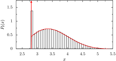
Figure 4: Theory versus numerics. We show the probability density $P_{t}(x)$ as a function of the coordinate $x$ for $f=1$, $g=0.3$, $\lambda=1$, and time $t=4$. The solid line (red online) represents the theoretical result obtained from Eqs. (28)-(31), while the histogram refers to our numerical simulation of Eq. (1).

Because the minimal and maximal velocities of the particles are $f-g$ and $f+g$, respectively, the regular part of the probability density, $\tilde{P}_{t}(x)$, is concentrated on the interval $[(f-g)t,(f+g)t]$. If $x$ belongs to this interval, then $\lim_{t\to 0}P_{t}(x)=\lambda(f-g)/2g$. For small but finite times $\tilde{P}_{t}(x)$ is an almost linear, decreasing function of $x$ which is transformed to a unimodal probability density as $t$ increases. These features of the probability density are illustrated in Fig. 3. In order to verify and test the theory for calculating $P_{t}(x)$, we performed as well direct numerical simulation of Eq. (1). As depicted in Fig. 4, our analytical results are in excellent agreement with the numerical findings.

V.1 Asymptotic Approach to a Gaussian Density

Based on the central limit theorem of probability theory, see, e.g., Ref. GK , we may expect that the probability density $P_{t}(x)$ tends to the normal (Gaussian) probability density as $t\to\infty$. To gain more insight into the long-time behavior of $P_{t}(x)$, we consider the scaled probability density defined by

$$\mathcal{P}_{t}(\xi)=\sigma_{t}P_{t}(\langle X_{t}\rangle+\sigma_{t}\xi)$$ (37)

which, in accordance with (24), can be written in the form

$$\mathcal{P}_{t}(\xi)=\frac{1}{2\pi}\int_{-\infty}^{\infty}\phi_{t}(u/\sigma_{t})\,e^{-iu\langle X_{t}\rangle/\sigma_{t}-iu\xi}du.$$ (38)

Assuming that $|u|\ll\sigma_{t}^{1/3}$ and keeping only the first two terms of the asymptotic expansion of the function $\phi_{t}(u/\sigma_{t})\,e^{-iu\langle X_{t}\rangle/\sigma_{t}}$ as $t\to\infty$, we obtain

$$\phi_{t}(u/\sigma_{t})\,e^{-iu\langle X_{t}\rangle/\sigma_{t}}=e^{-u^{2}/2}\bigg{[}1-i\frac{gu^{3}}{2\sqrt{\lambda f(f^{2}-g^{2})t}}\bigg{]}.$$ (39)

Substituting this formula into (38) yields $\mathcal{P}_{t}(\xi)=\mathcal{P}_{\infty}(\xi)+\mathcal{P}_{t}^{(1)}(\xi)$, where

$$\mathcal{P}_{\infty}(\xi)=\frac{1}{2\pi}\int_{-\infty}^{\infty}e^{-u^{2}/2-iu\xi}du=\frac{e^{-\xi^{2}/2}}{\sqrt{2\pi}}$$ (40)

is the probability density of the standard normal distribution and

$$\mathcal{P}_{t}^{(1)}(\xi)\!\! = \!\!-i\frac{g^{2}}{4\pi\lambda f^{2}}\int_{-\infty}^{\infty}e^{-u^{2}/2-iu\xi}u^{3}du$$ (41)

$$= \!\!-\frac{g(3\xi-\xi^{3})}{2\sqrt{\lambda f(f^{2}-g^{2})t}}\,\mathcal{P}_{\infty}(\xi)$$

($|\mathcal{P}_{t}^{(1)}(\xi)|/\mathcal{P}_{\infty}(\xi)\ll 1$) describes the deviation of $\mathcal{P}_{t}(\xi)$ from $\mathcal{P}_{\infty}(\xi)$. According to this result, $\mathcal{P}_{t}(\xi)$ slowly approaches ($\propto t^{-1/2}$) the asymptotic Gaussian form as $t\to\infty$.

A quantitative measure of non-Gaussian behavior of $P_{t}(x)$ can be characterized by the kurtosis defined as

$$k(t)=\frac{\langle(X_{t}-\langle X_{t}\rangle)^{4}\rangle}{\sigma_{t}^{4}}-3.$$ (42)

Notably, $k(t)$ is equal to zero if $X_{t}$ has the Gaussian distribution. Its dependence on time is calculated with the help of Eq. (32) and is depicted in Fig. 5. In accordance with the central limit theorem, the kurtosis tends to zero as $t$ increases. At very small times the formula (29) yields

$$P_{t}(x)=[1-\lambda(f-g)t]\,\delta[x-(f-g)t]+\frac{\lambda(f-g)}{2g},\;$$ (43)

where $x\in[(f-g)t,(f+g)t]$. For this probability density we readily obtain $\langle(X_{t}-\langle X_{t}\rangle)^{4}\rangle=(16/5)\lambda g^{4}(f-g)t^{5}$, $\sigma_{t}^{2}=(4/3)\lambda g^{2}(f-g)t^{3}$, and so $k(t)=(9/5)[\lambda(f-g)t]^{-1}$ as $t\to 0$. The divergence of kurtosis as $t\to 0$ corroborates the fact that at small times the probability density indeed strongly differs from the normal one.

The fact that $P_{t}(x)$ approaches asymptotically the normal probability density function with $\sigma_{t}^{2}\propto t$ as $t\to\infty$ leads to an interesting conclusion: Under certain conditions the long-time behavior of the considered particles is the same as the long-time behavior of Brownian particles. In order to elucidate this, we use the dimensionless equation of motion for overdamped Brownian particles: $\dot{x}_{t}=F+\xi(t)$ ($x_{0}=0$). Here, $x_{t}$ is the Brownian particle coordinate, $F$ is an external force, and $\xi(t)$ is Gaussian, thermal white noise with zero mean and correlation function $\overline{\xi(t)\xi(t^{\prime})}=2\Delta\delta(t-t^{\prime})$ (the overbar denotes an average over all realizations of $\xi(t)$ and $\Delta$ is the noise intensity). As is well-known, see, e.g., Refs. H-T ; V-K , $x_{t}$ has a Gaussian density with $\overline{x}_{t}=Ft$ and $\overline{(x_{t}-\overline{x}_{t})^{2}}=2\Delta t$. Therefore, the long-time statistical properties of usual Brownian particles and particles in our case are the same if $\overline{x}_{t}=\langle X_{t}\rangle$ and $\overline{(x_{t}-\overline{x}_{t})^{2}}=\sigma_{t}^{2}$, i.e., $F=(f^{2}-g^{2})/f$ and $\Delta=D_{\text{eff}}$. We further note that in the Brownian case the internal noise intensity $\Delta$ is proportional to the absolute temperature; thus, the long-time behavior of $X_{t}$ can also be characterized by the dimensionless effective temperature $T_{\text{eff}}=D_{\text{eff}}$.

V.2 Numerical Simulations

The numerical simulation of Eq. (1) turned out to be a valuable tool in verifying our analytical findings. We take advantage of the fact that this equation contains no explicit time dependent terms. In such a case, the numerical simulations can be made especially efficient. According to Eq. (1), inside each interval where $g(x)=-1$ or $+1$ the particle velocity is given by $f-g$ or $f+g$, respectively. Thus, the algorithm consists of successive generations of random interval lengths according to the exponential distribution and a calculation of the times needed to travel the generated interval with constant velocity $f-g$ or $f+g$. The total time is summed up until it reaches the required final value. The ensemble average is then obtained by repeating this outlined procedure with different realizations of random intervals. The probability density function is then obtained as the histogram of final positions of the particle. Using this method, we could obtain the probability density $P_{t}(x)$ with similar computational effort as the calculation of the Fourier integral (24). The averaging over $10^{7}$ realizations usually assumed several seconds on modern workstations. The existence of the $\delta$-singular part of $P_{t}(x)$ was recognized in our histogram-procedure by changing the bin size of the histogram: The number of counts in the histogram bin containing the $\delta$-function does not depend on the bin size.

VI DISCUSSION AND CONCLUSIONS

We used a path integral approach for determining the probability density function of overdamped particles in a piecewise linear random potential which are in addition driven by a constant force. Assuming that the intervals of the piecewise linear parts of the potential are distributed with an exponential distribution, we succeeded in obtaining the time-dependent probability density in the form of an explicit Fourier integral. Within this framework, we showed that the probability density contains, apart from a regular part, also a $\delta$-singular contribution. The weight of this $\delta$-singular part exponentially decreases with time and the total probability density slowly, as $t^{-1/2}$, converges to a Gaussian density in the long-time limit.

We further calculated the first and the second moments of the probability density function and studied its time evolution, both analytically and numerically. Our analytical results are in perfect agreement with the numerical ones obtained from simulations of the equation of motion. Moreover, we derived a simple representation of the probability density for small and large times and, to characterize the non-Gaussianity of the probability density, we calculated the kurtosis as a function of time. We showed that under certain conditions the long-time behavior of the considered particles is the same as Brownian particles. The corresponding effective diffusion coefficient and effective temperature are calculated.

Appendix A Proof of the normalization condition for $\textit{W}_{\textit{n}}\textbf{(}\textit{t}\textbf{)}$

Let us introduce the quantities

$$S_{n}(t)=\int_{\Omega_{n}(t)}\prod_{j=1}^{n}p(s_{j})ds_{j}$$ (44)

with $n\geq 1$. According to the definitions of $\Omega_{n}(t)$ and $\tilde{s}_{k}$, these quantities can be written in the form

$$S_{n}(t)=\int_{0}^{\tilde{s}_{1}}p(s_{1})ds_{1}\int_{0}^{\tilde{s}_{2}}p(s_{2})ds_{2}\ldots\int_{0}^{\tilde{s}_{n}}p(s_{n})ds_{n}.$$ (45)

Using in Eq. (8) the integral relation $\int_{\tilde{s}_{n+1}}^{\infty}p(s)ds=1-\int_{0}^{\tilde{s}_{n+1}}p(s_{n+1})ds_{n+1}$ resulting from the normalization condition for $p(s)$, we can express the probabilities $W_{n}(t)$ through the quantities $S_{n}(t)$ as follows:

$$W_{n}(t)=S_{n}(t)-S_{n+1}(t).$$ (46)

Taking also into account that $S_{\infty}(t)=0$, this representation of $W_{n}(t)$ yields $\sum_{n=1}^{\infty}W_{n}(t)=S_{1}(t)$. On the other hand, since $W_{0}(t)=1-S_{1}(t)$, we find that the normalization condition $W_{0}(t)+\sum_{n=1}^{\infty}W_{n}(t)=1$ holds true.

Appendix B Derivation of Eq. (28)

According to (25), the characteristic function $\phi_{t}(\eta)$ can be written in the form

$$\phi_{t}(\eta)=-e^{-(\lambda-i\eta)ft}[A(\eta)e^{(\lambda-i\eta)gt}+B(\eta)e^{-(\lambda-i\eta)gt}]$$ (47)

with

$$A(\eta)=\frac{1}{2\pi}\int_{-\infty}^{\infty}\frac{iz+y+2g(\lambda-i\eta)}{(z-z_{1})(z-z_{2})}\,e^{(iz+y)t}dz$$ (48)

and

$$B(\eta)=\frac{1}{2\pi}\int_{-\infty}^{\infty}\frac{\lambda(f-g)}{(z-z_{3})(z-z_{4})}\,e^{(iz+y)t}dz.$$ (49)

Applying the residue theorem for calculating the integrals in (48) and (49), we obtain

$$A(\eta)=i[\text{Res}\,\Psi(\eta;z_{1})+\text{Res}\,\Psi(\eta;z_{2})]\;$$

$$B(\eta)=i[\text{Res}\,\Phi(\eta;z_{3})+\text{Res}\,\Phi(\eta;z_{4})]\;.$$ (50)

Here, $\text{Res}\,\Psi(\eta;z_{1,2})$ and $\text{Res}\,\Phi(\eta;z_{3,4})$ are the residues of the functions

$$\displaystyle\Psi(\eta;z)=\frac{iz+y+2g(\lambda-i\eta)}{(z-z_{1})(z-z_{2})}\,e^{(iz+y)t},$$

$$\displaystyle\Phi(\eta;z)=\frac{\lambda(f-g)}{(z-z_{3})(z-z_{4})}\,e^{(iz+y)t}$$ (51)

of the complex variable $z$ at the points $z_{k}$. Assuming that $y>\lambda(f+g)$ (in this case $\text{Im}\,z_{k}>0$) and taking into account that $\text{Res}\,\Psi(\eta;z_{1,2})=\lim_{z\to z_{1,2}}(z-z_{1,2})\Psi(\eta;z)$ and $\text{Res}\,\Phi(\eta;z_{3,4})=\lim_{z\to z_{3,4}}(z-z_{3,4})\Phi(\eta;z)$, from Eqs. (50), (51) and (26) we find

$$A(\eta)\!\! = \!\!-e^{-(\lambda-i\eta)gt}\bigg{(}\frac{g(\lambda-i\eta)}{b(\eta)-ia(\eta)}\sinh{[b(\eta)t-ia(\eta)t]}$$

$$\!\!+\cosh{[b(\eta)t-ia(\eta)t]}\bigg{)},$$

$$B(\eta)\!\! = \!\!\frac{\lambda(g-f)}{b(\eta)-ia(\eta)}e^{(\lambda-i\eta)gt}\sinh{[b(\eta)t-ia(\eta)t]}.\quad\quad$$ (52)

Finally, substituting (52) into (47), we end up with (28).

Figure 1: Model potential and force field. (a) Schematic representation of the piecewise varying linear random potential $U(x)$ and (b) the corresponding dichotomous random force $g(x)=-dU(x)/dx$ as functions of the particle coordinate $x$.

Figure 2: (a) Behavior of the average velocity $\langle v\rangle$ and (b) of the effective diffusion coefficient $D_{\text{eff}}$ versus the external force $f$ for the chosen parameter values $\lambda=g=1$.

Figure 3: Time evolution of the probability density. Depicted are the plots of the probability density $P_{t}(x)$ derived from Eqs. (28)-(31) for the evolution time (a) $t=0.75$, (b) $t=2$, and (c) $t=5$. The values of the other parameters are set at $f=1$, $g=0.3$, and $\lambda=1$. The vertical arrows depict the singular parts of decreasing weight of $P_{t}(x)$.

Figure 5: Deviation from Gaussian behavior. The kurtosis $k(t)$ of the probability density is depicted on a linear [$k(t)$] versus logarithmic [$t$] scale as a function of the evolution time $t$ for $f=1$, $g=0.3$, and $\lambda=1$.

References

- (1) J. P. Bouchaud and A. Georges, Phys. Rep. 195, 127 (1990).
- (2) J. P. Bouchaud, A. Comtet, A. Georges, and P. Le Doussal, Ann. Phys. 201, 285 (1990).
- (3) S. Scheidl, Z. Phys. B 97, 345 (1995).
- (4) P. Le Doussal and V. M. Vinokur, Physica (Amsterdam) 254C, 63 (1995).
- (5) H. Horner, Z. Phys. B: Condens. Matter 100, 243 (1996).
- (6) D. A. Gorokhov and G. Blatter, Phys. Rev. B 58, 213 (1998).
- (7) S. I. Denisov and W. Horsthemke, Phys. Rev. E 62, 3311 (2000).
- (8) A. V. Lopatin and V. M. Vinokur, Phys. Rev. Lett. 86, 1817 (2001).
- (9) P. Reimann and P. Hänggi, Appl. Phys. A 75, 169 (2002).
- (10) R. D. Astumian and P. Hänggi, Phys. Today 55, No. 11, 33 (2002).
- (11) P. Hänggi, F. Marchesoni and F. Nori, Ann. Physik (Berlin) 14, 51 (2005).
- (12) F. Marchesoni, Phys. Rev. E 56, 2492 (1997).
- (13) M. N. Popescu, C. M. Arizmendi, A. L. Salas-Brito, and F. Family, Phys. Rev. Lett. 85, 3321 (2000).
- (14) L. Gao, X. Luo, S. Zhu, and B. Hu, Phys. Rev. E 67, 062104 (2003).
- (15) P. E. Parris, M. Kuś, D. H. Dunlap, and V. M. Kenkre, Phys. Rev. E 56, 5295 (1997).
- (16) V. M. Kenkre, M. Kuś, D. H. Dunlap, and P. E. Parris,, Phys. Rev. E 58, 99 (1998).
- (17) Ya. G. Sinai, Theory Probab. Appl. 27, 256 (1982).
- (18) A. O. Golosov, Commun. Math. Phys. 92, 491 (1984).
- (19) C. Monthus, Lett. Math. Phys. 78, 207 (2006).
- (20) P. Hänggi, P. Talkner, and M. Borkovec, Rev. Mod. Phys. 62, 251 (1990).
- (21) S. I. Denisov, J. Magn. Magn. Mater. 147, 406 (1995).
- (22) S. I. Denisov and R. Yu. Lopatkin, Phys. Scr. 56, 423 (1997).
- (23) A. P. Prudnikov, Yu. A. Brychkov, and O. I. Marichev, Integrals and Series (Gordon & Breach, New York, 1986), Vol. 1, Eq. 2.3.4.9.
- (24) B. V. Gnedenko and A. N. Kolmogorov, Limit Distributions for Sums of Independent Random Variables (Addison-Wesley, Cambridge, MA, 1954).
- (25) P. Hänggi and H. Thomas, Phys. Rep. 88, 207 (1982).
- (26) N. G. Van Kampen, Stochastic Processes in Physics and Chemistry (North-Holland, Amsterdam, 1992).