Descent Relations in Cubic Superstring Field Theory

Abstract:

The descent relations between string field theory (SFT) vertices are characteristic relations of the operator formulation of SFT and they provide self-consistency of this theory. The descent relations $\langle V_{2}|V_{1}\rangle$ and $\langle V_{3}|V_{1}\rangle$ in the $NS$ fermionic string field theory in the $\kappa$ and discrete bases are established. Different regularizations and schemes of calculations are considered and relations between them are discussed.

1 Introduction

The cubic open superstring field theory (SSFT) which keeps the main features of the Witten open bosonic string field theory [1] has the following action [2, 3]:

$$S=\mathchoice{{\vbox{\hbox{$\textstyle\diagup$}}\kern-6.52779pt}}{{\vbox{\hbox{$\scriptstyle\diagup$}}\kern-5.19446pt}}{{\vbox{\hbox{$\scriptscriptstyle\diagup$}}\kern-3.68056pt}}{{\vbox{\hbox{$\scriptscriptstyle\diagup$}}\kern-3.26389pt}}\!\int\Phi\star Q\Phi+\frac{2}{3}\mathchoice{{\vbox{\hbox{$\textstyle\diagup$}}\kern-6.52779pt}}{{\vbox{\hbox{$\scriptstyle\diagup$}}\kern-5.19446pt}}{{\vbox{\hbox{$\scriptscriptstyle\diagup$}}\kern-3.68056pt}}{{\vbox{\hbox{$\scriptscriptstyle\diagup$}}\kern-3.26389pt}}\!\int\Phi\star\Phi\star\Phi.$$ (1)

As in the bosonic SFT action the action (1) contains two main ingredients: a multiplication $\star$ and an integral $\mathchoice{{\vbox{\hbox{$\textstyle\diagup$}}\kern-6.52779pt}}{{\vbox{\hbox{$\scriptstyle\diagup$}}\kern-5.19446pt}}{{\vbox{\hbox{$\scriptscriptstyle\diagup$}}\kern-3.68056pt}}{{\vbox{\hbox{$\scriptscriptstyle\diagup$}}\kern-3.26389pt}}\!\int$. Comparing with its bosonic counterpart $\int$, $\mathchoice{{\vbox{\hbox{$\textstyle\diagup$}}\kern-6.52779pt}}{{\vbox{\hbox{$\scriptstyle\diagup$}}\kern-5.19446pt}}{{\vbox{\hbox{$\scriptscriptstyle\diagup$}}\kern-3.68056pt}}{{\vbox{\hbox{$\scriptscriptstyle\diagup$}}\kern-3.26389pt}}\!\int$ has an extra picture changing operator: $\mathchoice{{\vbox{\hbox{$\textstyle\diagup$}}\kern-6.52779pt}}{{\vbox{\hbox{$\scriptstyle\diagup$}}\kern-5.19446pt}}{{\vbox{\hbox{$\scriptscriptstyle\diagup$}}\kern-3.68056pt}}{{\vbox{\hbox{$\scriptscriptstyle\diagup$}}\kern-3.26389pt}}\!\int\equiv\int Y_{-2}$ [2, 3].

An appearance of the notion of pictures is a main novelty in the open SSFT. The pictures are the characteristics of the ghost sector of the fermionic string. We explain all specific of the appearance of picture changing operators in Section 2.

Representations of $\star$ and $\mathchoice{{\vbox{\hbox{$\textstyle\diagup$}}\kern-6.52779pt}}{{\vbox{\hbox{$\scriptstyle\diagup$}}\kern-5.19446pt}}{{\vbox{\hbox{$\scriptscriptstyle\diagup$}}\kern-3.68056pt}}{{\vbox{\hbox{$\scriptscriptstyle\diagup$}}\kern-3.26389pt}}\!\int$ in the operator and conformal languages were constructed in [4, 5, 6] (for a review see [7, 8, 9, 10]). Initially the vertices in the operator realization (both for the bosonic and for the fermionic strings) were built in the discrete basis (standard oscillator basis) and defined through the infinite dimensional Neumann matrices [4, 6]. Calculations using these vertices are rather complicated [11]. Rastelli, Sen and Zwiebach [16] suggested to transform vertices to the basis called $\kappa$-basis where $K_{1}=L_{1}+L_{-1}$ is diagonal. The formalism of the $\kappa$-basis has already proved its simplicity in [19]-[32].

In the operator representation of the theory (1) fields $\Phi$ are realized as ket-vectors $|\Phi\rangle$ in the Fock space. The multiplication and the integral can be given with the help of two vertices. The vertex $\langle|\hat{V}_{3}|\rangle$ represents $\star$:

$$|\Phi_{1}\star\Phi_{2}\rangle=\langle|\hat{V}_{3}|\rangle|\Phi_{1}\rangle|\Phi_{2}\rangle$$

and the vertex $\langle\hat{V}_{1}|$ represents $\mathchoice{{\vbox{\hbox{$\textstyle\diagup$}}\kern-6.52779pt}}{{\vbox{\hbox{$\scriptstyle\diagup$}}\kern-5.19446pt}}{{\vbox{\hbox{$\scriptscriptstyle\diagup$}}\kern-3.68056pt}}{{\vbox{\hbox{$\scriptscriptstyle\diagup$}}\kern-3.26389pt}}\!\int$:

$$\mathchoice{{\vbox{\hbox{$\textstyle\diagup$}}\kern-6.52779pt}}{{\vbox{\hbox{$\scriptstyle\diagup$}}\kern-5.19446pt}}{{\vbox{\hbox{$\scriptscriptstyle\diagup$}}\kern-3.68056pt}}{{\vbox{\hbox{$\scriptscriptstyle\diagup$}}\kern-3.26389pt}}\!\int\Phi=\langle\hat{V}_{1}|\Phi_{1}\rangle.$$

Having these vertices one can construct pure ”left” vertices $\langle\hat{V}_{2}|,$ $\langle\hat{V}_{3}|,$ $\langle\hat{V}_{4}|,$… etc. via natural definitions

$$\langle\hat{V}_{2}|=\langle\hat{V}_{1}|\langle|\hat{V}_{3}|\rangle,\,\,\langle\hat{V}_{3}|=\langle\hat{V}_{1}|\langle|\hat{V}_{3}|\rangle\langle|\hat{V}_{3}|\rangle,\,\,\langle\hat{V}_{4}|=\langle\hat{V}_{1}|\langle|\hat{V}_{3}|\rangle\langle|\hat{V}_{3}|\rangle\langle|\hat{V}_{3}|\rangle,...$$

These vertices form the so-called Witten tower of vertices [14]. They satisfy the descent relations which are written in terms of the “right” 1-vertex $|\hat{V}_{1}\rangle$ defined as a solution of the following relation

$$\langle\hat{V}_{2}||\hat{V}_{1}\rangle=\langle\hat{V}_{1}|.$$ (2)

One can prove [14] that the descent relations have the form

$$\langle\hat{V}_{n+1}||\hat{V}_{1}\rangle=\langle\hat{V}_{n}|.$$ (3)

In practice one usually construct the ”left” vertices $\langle V_{n}|$ by solving overlap conditions [4]. To stress the origin of these vertices we remove hats. It is obvious that the overlap conditions define vertices up to normalization factors $\langle\hat{V}_{n}|=Z_{n}\langle V_{n}|$ and $|\hat{V}_{1}\rangle=Z_{-1}|V_{1}\rangle$. Therefore the following modification of the descend relations (3) for $\langle V_{n}|$ takes place

$$\langle V_{n+1}\mid V_{1}\rangle=\mathcal{Z}_{n}\langle V_{n}|~{}~{}~{}~{}~{}\mathcal{Z}_{n}=Z_{n}Z_{-1}^{-1}Z_{n+1}^{-1}$$ (4)

These relations are indispensable ingredients of SFT, and they play important role in the SFT perturbation technique [11]. Note that the vertices $\hat{V}_{1}$ and $\hat{V}_{3}$ are defined up to two normalization factors as well. These factors can be absorbed into the charge and string field redefinitions in the cubic SFT action.

The descent relations are exact relations. Performing a check of the descent relations within a calculation scheme one performs a check of the calculation scheme itself. One can analyze

• operator structure of relations (4);

• numerical factors in (4).

There is no reason to expect that $\mathcal{Z}_{n}$ are well defined and therefore a regularization is needed. Different regularizations are suitable for different bases and one can expect different factors $\mathcal{Z}_{n}$ for different schemes and different regularizations. Moreover the $\mathcal{Z}_{n}$ is a product of factors coming from matter and ghost sectors separately. Each of these factors are singular ones tend to zero and another ones to infinity. One needs a special relation between matter and ghost regularizations to provide finite answers.

A study of the descent relations between string vertices in the bosonic string has been performed by Belov [12] and Fucks and Kroyter [13]. In ref. [12, 13, 14, 15] it was found that $\mathcal{Z}_{3}\neq 1$. The appearance of $\mathcal{Z}_{3}\neq 1$ in the descent relations was considered as an anomaly [13]. In [15] there was suggested the regularization for which the coefficient $\mathcal{Z}_{3}$ was equal one in the bosonic string. The factorization of the coefficient $\mathcal{Z}_{n}=Z_{n}Z_{-1}^{-1}Z_{n+1}^{-1}$ was found in the $\kappa$-basis [12], the origin of this factorization was revealed in [14].

In this paper we investigate the descent relations in the Neveu-Schwartz $(NS)$ sector of the fermionic string. Our goals are

• find a numerical factor in the relation $\langle V_{2}|V_{1}\rangle=\mathcal{Z}_{2}\langle V_{1}|$;

• check the descent relation $\langle V_{3}|V_{1}\rangle=\mathcal{Z}_{3}\langle V_{2}|$.

We check these relations in the $\kappa$-basis and in the discrete one and discuss the different regularizations in these bases. It is interesting to note that in contrast to the calculations in the bosonic string where all calculations in the discrete basis were performed only numerically [13, 14], some calculations in the fermionic sector can be performed analytically. Namely, we analytically calculate the Neumann matrix in the vertex $\langle V_{2}|$ through a multiplication the Neumann matrices of the vertices $\langle V_{3}|$ and $|V_{1}\rangle$.

This paper is organized as the following. In Section 2 we remind some aspects of the Fock representation of the superstring field theory and note special aspects of the descent relations for the NS string. In Section 3 we discuss some properties of the lowest vertices $V_{1}$ and $V_{2}$. In Section 4 we remind some features of the $\kappa$-basis for the $NS$ fermionic string and calculate the descent relation between vertices $\langle V_{3}|$ and $|V_{1}\rangle$. Here we also calculate the coefficient $\mathcal{Z}_{3}$. The descent relation $\langle V_{3}|V_{1}\rangle=\langle V_{2}|$ in the discrete basis is calculated in Section 5. In Section 6 we discuss the coefficients $\mathcal{Z}_{3}$ and an issue of regularizations.

2 Specific of Decent Relations in NS string

Let us remind the main features of the fermionic string. The ghost $\beta,~{}\gamma$ sector of the fermionic string has many different nonequivalent vacua $|q\rangle$ which are known as pictures and labeled by integers. Transitions between vacua (pictures) are realized by an infinite number of ghost modes. This is the difference between the ghost sector of the fermionic string and the ghost sector of the bosonic string where the transition between vacua is realized by one mode of ghost or anti-ghost. There is an operator which changes the picture:

$$|q\rangle=e^{q\phi(0)}|0\rangle,$$ (5)

where $\phi(z)$ is the field bozonizing the superghosts as $\beta=e^{-\phi}\partial\xi,~{}\gamma=e^{\phi}\eta$ [17]. The BRST-invariant operators realizing the transition between various vacua are called the picture changing operators [2, 3, 17, 18]. There are two picture changing operators $X$ and $Y_{-1}$ which change the picture $|q\rangle$ in the following way

$$X(|q\rangle) \Rightarrow |q+1\rangle,$$

$$Y_{-1}(|q\rangle) \Rightarrow |q-1\rangle.$$ (6)

Both these operators commute with BRST charge $Q$: $[X,Q]=0,\quad[Y_{-1},Q]=0,$ and obey the key property $(X\cdot Y_{-1})(z)=\lim_{z\to z^{\prime}}X(z)Y_{-1}(z^{\prime})=1$.

The normalization of the vacua has the form [17]

$$\langle-q-2|q\rangle=1.$$ (7)

In the action (1) one uses zero-picture string fields

$$|\Phi^{(0)}\rangle=\sum_{k,l,n\in\mathbb{N}\atop m,j,i\in\mathbb{N}+\frac{1}{2}}A_{i\dots}(x)\,\beta_{-i}...\gamma_{-j}...b_{-k}...c_{-l}...\alpha^{\mu}_{-n}...\psi^{\nu}_{-m}|0\rangle.$$ (8)

The vertex $\langle\hat{V}_{1}|$ defining the string integral for zero picture fields is a vector and has the picture “-2” and we denote it by the superscript “(-2)”

$$\mathchoice{{\vbox{\hbox{$\textstyle\diagup$}}\kern-6.52779pt}}{{\vbox{\hbox{$\scriptstyle\diagup$}}\kern-5.19446pt}}{{\vbox{\hbox{$\scriptscriptstyle\diagup$}}\kern-3.68056pt}}{{\vbox{\hbox{$\scriptscriptstyle\diagup$}}\kern-3.26389pt}}\!\int\Phi\equiv^{(-2)}\langle\hat{V}_{1}|\Phi^{(0)}\rangle.$$ (9)

Next one defines the star product $\star$ of two string fields as

$$|\Phi_{1}\star\Phi_{2}\rangle_{3}^{(0)}={}_{12}\langle|\hat{V}_{3}|\rangle_{3}|\Phi^{(0)}\rangle_{1}|\Phi^{(0)}\rangle_{2}.$$ (10)

Hence the vertex ${}_{12}\langle|\hat{V}_{3}|\rangle_{3}$ in (10) has the pictures “-2”, “-2” and “0” respectively, so we denote it as ${}^{(-2,-2)}{}_{12}\langle|V_{3}|\rangle_{3}^{(0)}$.

Using the vertices ${}^{(-2)}\langle\hat{V}_{1}|$ and ${}^{(-2,-2)}{}_{12}\langle|\hat{V}_{3}|\rangle_{3}^{(0)}$ one can build a vertex $\langle\hat{V}_{2}|$ as

$${}^{(-2,-2)}{}_{12}\langle\hat{V}_{2}|\equiv{}^{(-2)}{}_{3}\langle\hat{V}_{1}|^{(-2,-2)}{}_{12}\langle|\hat{V}_{3}|\rangle_{3}^{(0)}.$$ (11)

Now we are able to define a vertex $|\hat{V}_{1}\rangle$ as a solution of eq. (2) with $|\hat{V}_{1}\rangle$ in the zero picture:

$${}^{(-2,-2)}{}_{12}\langle\hat{V}_{2}|\hat{V}_{1}\rangle_{2}^{(0)}\equiv{}^{(-2)}{}_{1}\langle\hat{V}_{1}|.$$ (12)

One can build an infinite tower of vertices ${}_{1\dots N}\bigl{\langle}|\hat{V}_{N+1}|\bigr{\rangle}_{N+1}$ by gluing of $N-1$ vertices  $\hat{V}_{3}$. They have $N$ vacua in the picture “-2” and one vacuum in the picture “0”. Using the vertex ${}_{1\dots N}\bigl{\langle}|\hat{V}_{N+1}|\bigr{\rangle}_{N+1}$, one can define the star product for $N$ fields as:

$${}^{(-2,-2,...-2)}{}_{1\dots N}\bigl{\langle}|\hat{V}_{N+1}|\bigr{\rangle}^{(0)}_{N+1}|\Phi^{(0)}_{N}\rangle\dots|\Phi^{(0)}_{1}\rangle\equiv|\Phi_{N}^{(0)}\rangle\star\dots\star|\Phi_{1}^{(0)}\rangle.$$ (13)

By an analogy with the bosonic case one can also build an infinite tower of the vertices ${}^{(-2,...,-2)}{}_{1\dots N}\langle\hat{V}_{N}|$ associated with the vertices ${}^{(-2,...-2)}{}_{1\dots N}\langle|\hat{V}_{N+1}|\rangle_{N+1}^{(0)}$ constructed above by adding one more ${}^{(-2)}\langle\hat{V}_{1}|$ as in (11). Like we did it [14] in the bosonic string, let us call this set of the vertices Witten’s tower of vertices. Therefore one has the descent relations between the vertices $\langle\hat{V}_{N+1}|$ and $\langle\hat{V}_{N}|$ [14]:

$${}^{(-2,...,-2)}\langle\hat{V}_{N+1}|\hat{V}_{1}\rangle^{(0)}={}^{(-2,...,-2)}\langle\hat{V}_{N}|.$$ (14)

As has been mentioned in the introduction in practice one defines $\langle V_{N}|$ via the overlap conditions that define corresponding vertices up to numerical factors. Moreover, in practice defining a vertex via these overlap conditions one can use different realizations of pictures. For example, ${}^{(-2,-2)}\langle V_{2}|$ can be presented with help of an operator acting on a bra vacuum vector $\langle-2|\langle-2|$

$${}^{(-2,-2)}\langle V_{2}|=\langle-2|{}\langle-2|\,\,{\cal V}_{-2,-2},$$ (15)

as well as result of acting of the picture changing operator $Y_{-1}Y_{-1}$ (in different points) on a vector $\langle-1|\langle-1|\,\,{\cal V}_{-1,-1}$,

$${}^{(-2,-2)}\langle V_{2}|=\langle-1|\langle-1|\,\,{\cal V}_{-1,-1}\,\,Y_{-1}Y_{-1},$$ (16)

or

$${}^{(-2,-2)}\langle V_{2}|=\langle 0|\langle-2|\,\,{\cal V}_{0,-2}\,\,Y_{-2},$$ (17)

with $Y_{-2}$ being $Y_{-2}|q\rangle\Rightarrow|q-2\rangle$.

It is difficult to treat $Y_{-1}$ in operator formalisms [18] and therefore, it is difficult to check explicitly that these representations (15), (16) and (17) are equivalent (see also [33]). As for the descent relation ${}^{(-2,-2,-2)}\langle V_{3}|V_{1}\rangle^{(0)}\simeq{}^{(-2,-2)}\langle V_{2}|$ we will check it for vertices in the form ${}^{(-2,-2,-2)}\langle V_{3}|=\langle-1|\langle-1|\langle-2|\mathcal{V}_{-1,-1,-2}Y_{-1}Y_{-1}$ and ${}^{(-2,-2)}\langle V_{2}|=\langle-1|\langle-1|\mathcal{V}_{-1,-1}Y_{-1}Y_{-1},$ i.e. we have to check

$$\langle-1|\langle-1|\langle-2|\mathcal{V}_{-1,-1,-2}Y_{-1}Y_{-1}|V_{1}\rangle=\langle-1|\langle-1|\mathcal{V}_{-1,-1}Y_{-1}Y_{-1}.$$ (18)

We can assume that $Y_{-1}$-’s acts on one “external” legs 1, or 2 in (18) and remove $Y_{-1}Y_{-1}$ that gives

$${}^{(-1,-1,-2)}\langle V_{3}|V_{1}\rangle^{(0)}\simeq{}^{(-1,-1)}\langle V_{2}|.$$ (19)

The same is true for $|V_{1}\rangle$ defining relation. We actually check

$${}^{(-2,0)}\langle V_{2}|V_{1}\rangle^{(0)}={}^{(0)}\langle V_{1}|$$

as

$${}^{(-2,-2)}\langle V_{2}|V_{1}\rangle^{(0)}={}^{(-2)}\langle V_{1}|$$

in a special form is equivalent to

$$\langle-2,0|\mathcal{V}_{-2,0}Y_{-2}|V_{1}\rangle=\langle 0|\mathcal{V}_{0}Y_{-2}$$

Therefore for checking the descent relations we have a freedom to choose the vertices in the pictures which are more convenient for the calculations.

3 $V_{1}$ and $V_{2}$

The solution $|V_{1}\rangle$ of the defining equation (12) is unique, that can be transparently exemplified on the bosonic vertex $|V_{1}^{X}\rangle$. To show this it is enough to check that $\langle V_{2}|$ is nondegenerated. In the case of bosonic string

$$\langle V_{2}^{X}|={}_{1,2}\langle 0|\exp(-a^{1}Ca^{2}),$$ (20)

where $[a_{n},a^{{\dagger}}_{m}]=\delta_{nm}$ are the modes of the string $X(\sigma)$ and $C_{nm}=(-1)^{n}\delta_{nm}$ (here we omit the zero mode for simplicity). Reminding the correspondence between a string field $\Phi[X(\sigma)]$ and a state $|\Phi\rangle$:

$$\Phi[X(\sigma)]\equiv\langle X(\sigma)|\Phi\rangle$$ (21)

we write the Dirac conjugation

$$\overline{\Phi}[X(\sigma)]=\langle\Phi|X(\sigma)\rangle.$$ (22)

Considering the vertex $\langle V_{2}^{X}|$ as an operator mapping ket-s $|\Phi\rangle$ to bra-s $\langle\Phi^{R}|$

$${}_{2}\langle\Phi^{R}|\equiv{}_{1,2}\langle V_{2}|\Phi\rangle_{1}$$ (23)

we write using (22):

$$\overline{\Phi}^{R}[X(\sigma)]={}_{1,2}\langle V_{2}|\Phi\rangle_{1}|X(\sigma)\rangle_{2}.$$ (24)

We calculate (for $E^{-1}_{nm}$ see [4])

$${}_{1,2}\langle V_{2}|X(\sigma)\rangle_{2} = {}_{1,2}\langle 0|\exp(-a_{n}^{1}(-1)^{n}a_{n}^{2})\exp\left(-x_{n}E^{-2}_{nn}x_{n}-2ia^{1{\dagger}}_{n}E^{-1}_{nn}x_{n}+\frac{1}{2}a^{1{\dagger}}_{n}a^{1{\dagger}}_{n}\right)|0\rangle_{1}$$

$$= {}_{2}\langle 0|\exp\left(-x_{n}E^{-2}_{nn}x_{n}+2i(-1)^{n}a^{2}_{n}E^{-1}_{nn}x_{n}+\frac{1}{2}(-1)^{n}a^{2}_{n}(-1)^{n}a^{2}_{n}\right)$$

$$= {}_{2}\langle 0|\exp\left(-((-1)^{n}x_{n}E^{-2}_{nn}(-1)^{n}x_{n})+2ia^{2}_{n}E^{-1}_{nn}(-1)^{n}x_{n}+\frac{1}{2}a^{2}_{n}a^{2}_{n}\right).$$

Taking into account the string modes expansion $X(\sigma)=i\sqrt{2}\sum_{n}x_{n}\cos(n\sigma)$ one gets

$${}_{1,2}\langle V_{2}|X(\sigma)\rangle_{2}=\langle X(\pi-\sigma)|.$$

That gives

$$\overline{\Phi}^{R}[X(\sigma)]=\langle X(\pi-\sigma)|\Phi\rangle=\Phi[X(\pi-\sigma)].$$ (26)

There is a string field decomposition

$$\Phi[X(\sigma)]=\Phi_{S}[X(\sigma)]+\Phi_{A}[X(\sigma)]$$

into the symmetric part

$$\Phi_{S}[X(\sigma)]=\Phi_{S}[X(\pi-\sigma)]$$

and the antisymmetric part

$$\Phi_{A}[X(\sigma)]=-\Phi_{A}[X(\pi-\sigma)].$$

Under this decomposition we have

$$\Phi^{R}[X(\sigma)]=\overline{\Phi}_{S}[X(\sigma)]-\overline{\Phi}_{A}[X(\sigma)].$$ (27)

Hence, we see that $\langle V_{2}|$ acts as the mapping

$$\langle V_{2}|:\quad\Phi[X(\sigma)]=\Phi_{S}[X(\sigma)]+\Phi_{A}[X(\sigma)]\to\overline{\Phi}_{S}[X(\sigma)]-\overline{\Phi}_{A}[X(\sigma)].$$ (28)

This mapping is nondegenerate and by this reason the solution of (12) is unique.

Taking $\langle V_{2}|$ as a quadratic form in the space of the string functional $(\Phi,\Phi)\equiv{}_{1,2}\langle V_{2}|\Phi\rangle_{1}|\Phi\rangle_{2}$ one sees that this metrics is neither positive defined nor nondegenerate. Indeed,

$$\langle V_{2}|\Phi\rangle|\Phi\rangle = \langle\Phi^{R}|\Phi\rangle=\langle\overline{\Phi}_{S}-\overline{\Phi}_{A}|\Phi_{S}+\Phi_{A}\rangle=$$ (29)

$$= \langle\overline{\Phi}_{S}|\Phi_{S}\rangle-\langle\overline{\Phi}_{A}|\Phi_{A}\rangle+\langle\overline{\Phi}_{S}|\Phi_{A}\rangle-\langle\overline{\Phi}_{A}|\Phi_{S}\rangle=$$

$$= \langle\overline{\Phi}_{S}|\Phi_{S}\rangle-\langle\overline{\Phi}_{A}|\Phi_{A}\rangle.$$

A few comments concerning $|V_{1}\rangle$ are in order. Let us multiply both sides of (12) by an arbitrary field $|\Phi\rangle$ and rewrite it in the Witten notations

$$\int V_{1}\star\Phi=\int\Phi,$$ (30)

where $V_{1}$ stand for a string field corresponding to $|V_{1}\rangle$ by $V_{1}[X(\sigma)]\equiv\langle X(\sigma)|V_{1}\rangle$. Since $\Phi$ is an arbitrary field one can discard the integral to get

$$V_{1}\star\Phi=\Phi.$$ (31)

Thus we conclude that $V_{1}$ defined by (12) is nothing but the unity under the star multiplication [4, 34, 35, 36].

Multiplying both sides of (23) by $|V_{1}\rangle$ from the right one gets

$$\langle V_{2}|\Phi\rangle|V_{1}\rangle=\langle\Phi^{R}|V_{1}\rangle,$$ (32)

that gives via descent relation (12)

$$\langle V_{1}|\Phi\rangle=\langle\Phi^{R}|V_{1}\rangle.$$ (33)

In order to have the positively defined and nondegenerate quadratic form (29) we put the following constraints on the symmetric and antisymmetric field parts:

$$\Phi_{S}=\overline{\Phi}_{S},$$ i.e the symmetric part is a real one,

$$\Phi_{A}=-\overline{\Phi}_{A},$$ i.e the antisymmetric part is an imaginary one, (34)

or for the field $\Phi$ we get

$$\Phi[X(\sigma)]=\Phi^{R}[X(\sigma)].$$ (35)

Following [1, 37] we call these fields as real. We see that on the linear subspace of the real string field $\langle V_{2}^{X}|$ acts as a unity operator i.e. $\langle V_{2}^{X}|\Phi\rangle=(|\Phi\rangle)^{+}$. The interesting question arises if the subspace of the real field is a subspace under $\star$ multiplication.

Hence, turning back to (33) we have for the real fields

$$\langle V_{1}|\Phi\rangle=\langle\Phi|V_{1}\rangle.$$ (36)

Thus, we conclude that $|V_{1}\rangle$ is both the identity for $\star$ and the ket representation of the Witten integral for the real string fields (35).

We start our calculation with the defining relation (12) for the fermionic variables $\psi$. By the direct calculation we check (12) for given vertices [4, 33].

The vertex $|V_{1}^{\psi}\rangle$ has the form [4]

$$|V_{1}^{\psi}\rangle=\exp\left\{\frac{1}{2}\sum_{r,s\geq 1/2}\psi_{-r}^{\mu}I_{rs}\psi_{-s}^{\mu}\right\}|0\rangle=\exp\left(\frac{1}{2}\psi I\psi\right)|0\rangle,$$ (37)

where $I_{rs}$ is the antisymmetric matrix (see Appendix, eq. (1)).

The vertex $\langle V_{2}^{\psi}|$ reads [4]

$$\langle V_{2}^{\psi}|={}_{12}\langle 0|\exp\left(-i\sum_{r\geq 1/2}\psi^{1}_{r}(-)^{r}\psi^{2}_{r}\right)={}_{12}\langle 0|\exp(-\psi^{1}S\psi^{2}),$$ (38)

where $S_{rs}=i(-1)^{r}\delta_{r,s}$.

So we have

$$\langle V_{2}^{\psi}|V_{1}^{\psi}\rangle={}_{12}\langle 0|\exp(-\psi^{1}S\psi^{2})\exp(\frac{1}{2}\psi^{1}I\psi^{1})|0\rangle_{1}.$$ (39)

We use the following identity [38]

$$\langle 0|\exp\left\{\frac{1}{2}\psi_{r}V_{rs}\psi_{s}+\psi_{r}\lambda_{r}\right\}\exp\left\{\frac{1}{2}\psi_{-r}I_{rs}\psi_{-s}\right\}|0\rangle$$

$$=\det(1+VI)^{1/2}\exp\left\{\frac{1}{2}\lambda_{r}(1+IV)^{-1}I_{rs}\lambda_{s}\right\}.$$ (40)

We get

$$\langle V_{2}^{\psi}|V_{1}^{\psi}\rangle=\langle 0|\exp\left(-\frac{1}{2}\psi_{r}^{2}(-1)^{r+p}I_{rp}\psi^{2}_{p}\right)=\langle V_{1}^{\psi}|.$$ (41)

For the superghost sector we can also calculate $\langle V_{2}|V_{1}\rangle$. The vertex $|V_{1}^{\beta\gamma}\rangle$ reads [4].

$$|V_{1}^{\beta\gamma}\rangle=\exp\left(\sum_{r\geq 3/2\atop s\geq-1/2}\beta_{-r}K_{rs}\gamma_{-s}\right)|0\rangle.$$ (42)

The vertex $\langle V_{2}|$ has the following form [33]

$$\langle V_{2}^{\beta\gamma}|={}_{1,2}\langle-2,0|\exp\left(i\sum_{r\geq-1/2}(-1)^{r}\gamma_{r}^{2}\beta_{r}^{1}-i\sum_{r\geq 3/2}(-1)^{r}\gamma_{r}^{1}\beta_{r}^{2}\right).$$ (43)

The descent relation is the following

$$\langle V_{2}^{\beta\gamma}|V_{1}^{\beta\gamma}\rangle={}_{1,2}\langle-2,0|\exp\left(i\sum_{r\geq-1/2}(-1)^{r}\gamma_{r}^{2}\beta_{r}^{1}-i\sum_{r\geq 3/2}(-1)^{r}\gamma_{r}^{1}\beta_{r}^{2}\right)\times$$

$$\times\exp\left(\sum_{r\geq 3/2\atop s\geq-1/2}\beta_{-r}^{1}K_{rs}\gamma_{-s}^{1}\right)|0\rangle_{1}.$$ (44)

We use the following identity [39]

$$\langle-2|\exp\{-\beta_{r}S_{rs}\gamma_{s}+\lambda_{s}\gamma_{s}+\beta_{s}\mu_{s}\}\exp\{\beta_{-r}V_{rs}\gamma_{-s}+\beta_{-s}\nu_{s}+\kappa_{s}\gamma_{-s}\}|0\rangle$$ (45)

$$=\det(1-SV)^{-1}\exp\{\kappa(1-SV)^{-1}(S\nu-\mu)-\lambda(1-VS)^{-1}(V\mu-\nu)\}.$$

So we get

$$\langle V_{2}^{\beta\gamma}|V_{1}^{\beta\gamma}\rangle=\langle 0|\exp\left(-\sum_{r\geq 3/2\atop s\geq-1/2}\beta_{r}^{2}(-1)^{r+s}K_{rs}\gamma_{s}^{2}\right)=\langle V_{1}^{\beta\gamma}|.$$ (46)

Here we got that the vertices $|V_{1}^{\psi}\rangle$ and $|V_{1}^{\beta\gamma}\rangle$ satisfy the defining equation (12) (the vertices $|V_{1}^{\psi}\rangle$ and $|V_{1}^{\beta\gamma}\rangle$ were got as the solution of the overlap equation). We also got the coefficient $\mathcal{Z}_{2}$ equal to one.

4 Descent relation in the $\kappa$-basis

4.1 $\kappa$-basis. General

The excellent description of the $\kappa$-basis for the fields of an arbitrary conformal weight $s$ was given in [21]. For the $NS$ sector of superstring we will be interested in the case $s=1/2$. In this section we review the notations and the main formulas from [21, 29].

Let $\mathcal{H}_{s}$ be the Hilbert space of analytic functions inside the unit disk and square-integrable on the boundary. The inner product for $f,g\in\mathcal{H}_{s}$ is given by

$$\langle g|f\rangle_{s}=\frac{1}{\pi\Gamma(2s-1)}\,\int_{|z|\leqslant 1}d^{2}z\,\bigl{[}1-z\bar{z}]^{2s-2}\,\overline{g(z)}f(z).$$ (47)

In our case $s=1/2$. The apparent singularity at $s=\frac{1}{2}$ is spurious [40].

The usual oscillator basis diagonalizes the generator $L_{0}$, which has discrete eigenvalues $(m+s)$, $m=0,1,2,\dots$. Its eigenfunctions normalized by (47) are

$$|m,s\rangle(z)=N_{m}^{(s)}z^{m}\quad\text{with}\quad N_{m}^{(s)}=\left[\frac{\Gamma(m+2s)}{\Gamma(m+1)}\right]^{1/2}.$$ (48)

For $s=1/2$ the normalization factor $N_{m}^{(1/2)}$ equals to one and $|m,1/2\rangle(z)=z^{m}$.

The vertices $\langle V_{N}|$ are $K_{n}$ symmetrical ones

$$\langle V_{3}|(K^{(1)}_{n}+K^{(2)}_{n}+K^{(3)}_{n}) = 0,$$ (49)

where $K_{n}=L_{n}-(-)^{n}L_{-n}$ and $L_{n}$ are the Virasoro generators. It is important that for $n=even$ only the full (matter+ghost) vertex (49) is $K_{n}$-invariant, but for $n=odd$ the vertices are invariant in the matter and ghost sectors [4, 16] separately. For $n-odd$ the $K_{n}$ invariance of a vertex means that the Neumann matrices $V_{kl}$ and the matrix corresponding to the operator $K_{n}$ commute (choose $n=1$):

$$[K_{1},V]=0.$$ (50)

Therefore, if one finds the eigenvectors of the matrix $K_{1,kl}$ and chooses them as basis vectors then the Neumann matrices are reduced to the diagonal form [16, 21, 25, 29, 30]. The calculations are greatly simplified in this basis [16, 21].

One can search for eigenfunctions of $K_{1}$ on the complex plane $z$, but it is convenient to use the map [16]

$$z=i\tanh w,$$ (51)

which takes the unit disk into the strip $|\text{Im}~{}w|\leq\pi/4$. In $w$ coordinate the operator $K_{1}$ takes the form

$$K_{1}=-i\frac{d}{dw}+i\tanh w.$$ (52)

The eigenvalues of the operator are all of the real numbers $\kappa$. The eigenfunctions of (52) are

$$|\kappa,1/2\rangle(z)=\bigl{[}A_{1/2}(\kappa)\bigr{]}^{1/2}\,\cosh w(z)\,e^{i\kappa w(z)},$$ (53)

where

$$A_{1/2}(\kappa)=\frac{1}{2\cosh\frac{\pi\kappa}{2}}$$

is the normalization constant, it is determined from

$$\langle\kappa,1/2|\kappa^{\prime},1/2\rangle=\delta(\kappa-\kappa^{\prime}).$$ (54)

The transformation “matrix” between the discrete and continuous bases is

$$\langle m,1/2|\kappa,1/2\rangle=V^{(1/2)}_{m}(\kappa)(A_{1/2}(\kappa))^{\frac{1}{2}}.$$ (55)

Here the polynomials $V^{(1/2)}_{m}(\kappa)$ are given by the generating function

$$\cosh w\,e^{i\kappa w}=\sum_{m=0}^{\infty}V_{m}^{(1/2)}(\kappa)z^{m}.$$ (56)

4.2 Matter sector

4.2.1 Matter sector in the $\kappa$-basis

Let $\psi(z)$ be a field of dimension $s=1/2$. In the $NS$ sector it has a half-integer mode expansion. Following [21, 29, 34] we decompose it into creation and annihilation parts with respect to the $SL(2,\mathbb{R})$-invariant vacuum $|0\rangle$:

$$\psi(z) = \sum_{n=0}^{\infty}\left[\psi_{-(n+\frac{1}{2})}\,z^{n}+\psi_{n+\frac{1}{2}}z^{-n-1}\right]$$ (57)

$$= \sum_{n=0}^{\infty}\left[\psi_{-(n+\frac{1}{2})}\,|1/2,n\rangle(z)+\psi_{n+\frac{1}{2}}|1/2,n\rangle(1/z)z^{-1}\right].$$

Using the completeness condition

$$\text{Id}(z,1/z)=\int_{\mathbb{R}}d\kappa|\kappa,1/2\rangle(z)\otimes\langle\kappa,1/2|(1/z)$$

and (55), one gets

$$\psi(z)=\int_{\mathbb{R}}d\kappa\sum_{n=0}^{\infty}(A_{1/2}(\kappa))^{\frac{1}{2}}\left[V^{(1/2)}_{n}(\kappa)\psi_{-(n+\frac{1}{2})}|\kappa,1/2\rangle(z)+V^{(1/2)}_{n}(\kappa)\psi_{n+\frac{1}{2}}|\kappa,1/2\rangle(1/z)z^{-1}\right],$$

or if one introduces the notation

$$\psi^{\pm}(\kappa)=\sqrt{A_{1/2}(\kappa)}\,\sum_{m=0}^{\infty}V_{m}^{(1/2)}(\kappa)\,\psi_{\mp(m+1/2)},$$ (58)

we have

$$\psi(z)=\int_{\mathbb{R}}d\kappa\left[\psi^{+}(\kappa)|\kappa,1/2\rangle(z)+\psi^{-}(\kappa)|\kappa,1/2\rangle(1/z)z^{-1}\right].$$

The anticommutation relations between the oscillators in $\kappa$-basis are

$$\{\psi^{-}(\kappa),\,\psi^{+}(\kappa^{\prime})\}=\delta(\kappa-\kappa^{\prime}).$$ (59)

4.2.2 $\langle V_{3}^{\psi}|V_{1}^{\psi}\rangle$ in the $\kappa$-basis

In this section we will consider the descent relation $\langle V_{3}^{\psi}|V_{1}^{\psi}\rangle$ for the matter sector of the $NS$ string in the $\kappa$-basis [29, 30].

The right identity $|V_{1}^{\psi}\rangle$ in the $\kappa$-basis [29] reads

$$|V_{1}^{\psi}\rangle=\exp\left\{-\frac{1}{2}\int_{0}^{\infty}d\kappa\tau(\kappa)\psi_{\alpha}^{+}(\kappa)\varepsilon_{\alpha\beta}\psi_{\beta}^{+}(\kappa)\right\}|0\rangle,\quad\alpha,\beta=1,2$$ (60)

where $\tau(\kappa)=\tanh(\frac{\pi\kappa}{4})$ and $\psi_{\alpha}^{+}(\kappa)$ is the two component vector

$$\psi_{1}^{\pm}(\kappa) = \frac{1}{\sqrt{2}}(\psi^{\pm}(\kappa)-\psi^{\pm}(-\kappa)),$$

$$\psi_{2}^{\pm}(\kappa) = \frac{1}{\sqrt{2}}(\psi^{\pm}(\kappa)+\psi^{\pm}(-\kappa)),$$

and

$$\varepsilon_{\alpha\beta}=\left(\begin{array}[]{cc}0&1\\ -1&0\\ \end{array}\right).$$

The $|\,0\rangle$ stands for the usual oscillator vacuum, it doesn’t change under transformation from the discrete basis to the $\kappa$-basis.

The three-string vertex is [29]

$$\langle V_{3}^{\psi}|={}_{123}\langle 0|\exp\left\{-\frac{1}{2}\int_{0}^{\infty}d\kappa\psi_{\alpha}^{a-}(\kappa)V_{\alpha\beta}^{ab}(\kappa)\psi_{\beta}^{b-}(\kappa)\right\},\quad a,b=1,2,3$$ (61)

where $V_{\alpha\beta}^{ab}(\kappa)$ is $6\times 6$ matrix defined by

$$V_{\alpha\beta}^{ab}(\kappa)=\mu(\kappa)\varepsilon_{\alpha\beta}\otimes\delta^{ab}+\mu_{t}(\kappa)c_{\alpha\beta}\otimes\chi^{ab}+\mu_{s}(\kappa)\varepsilon_{\alpha\beta}\otimes\epsilon^{ab};$$ (62)

$$\mu=\tau\frac{1-\tau^{2}}{1+3\tau^{2}},\quad\mu_{t}=\frac{1+\tau^{2}}{1+3\tau^{2}},\quad\mu_{s}=-\tau\frac{1+\tau^{2}}{1+3\tau^{2}},$$

and

$$c_{\alpha\beta}=\left(\begin{array}[]{cc}1&0\\ 0&-1\\ \end{array}\right).$$

We use the following notations [27]

$$\chi^{ab}=\left(\begin{array}[]{ccc}0&1&-1\\ -1&0&1\\ 1&-1&0\\ \end{array}\right),\qquad\epsilon^{ab}=\left(\begin{array}[]{ccc}0&1&1\\ 1&0&1\\ 1&1&0\\ \end{array}\right).$$

Hence, all the vertices are defined. We can evaluate the descent relation

$$\langle V_{3}^{\psi}|V_{1}^{\psi}\rangle =$$

$$= {}_{123}\langle 0|\exp\left\{-\frac{1}{2}\int_{0}^{\infty}d\kappa\psi_{\alpha}^{a-}(\kappa)V_{\alpha\beta}^{ab}(\kappa)\psi_{\beta}^{b-}(\kappa)\right\}$$

$$\times \exp\left\{-\frac{1}{2}\int_{0}^{\infty}d\kappa^{\prime}\tau(\kappa^{\prime})\psi_{\alpha}^{1+}(\kappa^{\prime})\varepsilon_{\alpha\beta}\psi_{\beta}^{1+}(\kappa^{\prime})\right\}|0\rangle_{1},$$

we use the formula of multiplication of two exponents in [29, 38]

$$= \det(1-\mu\tau(\kappa))^{10}$$

$$\times {}_{23}\langle 0|\exp\left\{-\frac{1}{2}\int_{0}^{\infty}d\kappa\psi_{\alpha}^{n-}(\kappa)\left[V_{\alpha\beta}^{nm}(\kappa)-V_{\alpha\gamma}^{n1}(\kappa)\frac{\tau(\kappa)}{1-\mu\tau(\kappa)}\varepsilon_{\gamma\delta}V_{\delta\beta}^{1m}(\kappa)\right]\psi_{\beta}^{m-}(\kappa)\right\}.$$

Here $\det(1-\mu\tau(\kappa))^{10}$ stands for the determinated of the diagonal operator $(1-\mu\tau(\kappa))\delta(k-k^{\prime})$.

Let us introduce the notation

$$U_{\alpha\beta}^{nm}(\kappa)=V_{\alpha\beta}^{nm}(\kappa)-V_{\alpha\gamma}^{n1}(\kappa)\frac{\tau(\kappa)}{1-\mu\tau(\kappa)}\varepsilon_{\gamma\delta}V_{\delta\beta}^{1m}(\kappa),\qquad m=2,3.$$ (63)

It is easy to check using the explicit expression of the matrix $V^{ab}(\kappa)$ (62) that the matrix $U_{\alpha\beta}^{nm}(\kappa)$ has the form

$$U_{\alpha\beta}^{22}(\kappa)=U_{\alpha\beta}^{33}(\kappa)=0,\quad\text{and}\quad U_{\alpha\beta}^{23}(\kappa)-U_{\beta\alpha}^{32}(\kappa)=2c_{\alpha\beta}.$$ (64)

Thus we get the following form for the vertex $\langle V_{2}|$

$$\langle V_{2}^{\psi}|={}_{12}\langle 0|\exp\left\{-\int_{0}^{\infty}d\kappa\psi_{\alpha}^{1-}(\kappa)c_{\alpha\beta}\psi_{\beta}^{2-}(\kappa)\right\}.$$ (65)

Thereby,

$$\langle V_{3}^{\psi}|V_{1}^{\psi}\rangle = \det(1-\mu\tau(\kappa))^{10}{}_{23}\langle 0|\exp\left\{-\int_{0}^{\infty}d\kappa\psi_{\alpha}^{2-}(\kappa)c_{\alpha\beta}\psi_{\beta}^{3-}(\kappa)\right\}$$ (66)

$$= \det(1-\mu\tau(\kappa))^{10}\langle V_{2}^{\psi}|.$$

We got the vertex $\langle V_{2}^{\psi}|$ and $\det(1-\mu\tau(\kappa))^{10}$ which is obviously divergent. Below we will show how to treat the determinant following [21].

To calculate $\det A$ one uses the standard trick

$$\det A=\exp\{\text{Tr}\log A\}.$$

Let us suppose that we have some operator $A$ which is diagonal in the $\kappa$-basis and has eigenvalues $A(\kappa)$

$$\text{Tr}~{}A=\int_{0}^{\infty}d\kappa\langle\kappa,1/2|A|1/2,\kappa\rangle=\int_{0}^{\infty}d\kappa A(\kappa)\langle\kappa,1/2|1/2,\kappa\rangle.$$ (67)

Taking into account (54) one gets

$$\text{Tr}A=\int_{0}^{\infty}d\kappa A(\kappa)\langle\kappa,1/2|1/2,\kappa\rangle\sim\delta(0)\int_{0}^{\infty}d\kappa~{}A(\kappa).$$ (68)

This expression diverges. One would like to regularize $\delta(0)$ and at first sight for this one can use any regularization of delta function. In [12, 21] the arguments were given how to choose the regularization. It was suggested to regularize the measure in the inner product (47) by $s\to s+\Delta$. The main argument for the regularization of measure was given through the associativity of operators $U_{p}$ which add the nonzero momentum to vertices. In [41] it was suggested that the anomaly in the associativity

$$\langle V_{N}|U_{p+q}=\langle V_{N}|(U_{p}U_{q})\neq(\langle V_{N}|U_{p})U_{q}$$

is connected with the breaking of the unitarity of the operator $U_{p}$. In order to act by the operator $U_{p}$ on a vertex it should be regularized. The regularization could break the unitarity. Manes used the level truncation method. Next in [42] the same calculation was done, but they used the regularization with the $\zeta$-function. They concluded that there is a regularization free from the anomaly. They suggested the complicated regularization in which the anomaly was absent. Using the $\Delta$ regularization of [12] it is easy to prove the associativity

$$\lim_{\Delta\to+0}\langle V_{N}|U_{q+p}^{(\Delta)}=\lim_{\Delta\to+0}\left[\lim_{\Delta^{\prime}\to+0}\langle V_{N}|U_{q}^{(\Delta^{\prime})}\right]U_{p}^{(\Delta)}.$$ (69)

It was suggested to introduce the spectral regularized density as

$$\rho_{s,\Delta}(\kappa^{\prime},\kappa)\equiv\langle\kappa^{\prime},s|\kappa,s\rangle_{s+\Delta}$$ (70)

and

$$\lim_{\Delta\to 0}\rho_{s,\Delta}(\kappa^{\prime},\kappa)=\rho_{s}(\kappa^{\prime},\kappa)=\delta(\kappa-\kappa^{\prime}).$$ (71)

Thus the regularized expression (68) can be written as

$$\text{Tr}_{\Delta}~{}A=\int_{0}^{\infty}d\kappa A(\kappa)\rho_{1/2,\Delta}(\kappa,\kappa).$$ (72)

So one can calculate the determinant of the operator through the trace of the operator with a regularized spectral density. The expression of the regularized spectral density for an arbitrary $s$ was found in [12]

$$\rho_{s,\Delta}(\kappa) = \frac{1}{4\pi\Delta}+\frac{\log 2}{2\pi}-B_{s}(\kappa),$$

where

$$B_{s}(\kappa)=\frac{1}{4\pi}\left[\psi\left(s+\frac{i\kappa}{2}\right)+\psi\left(s-\frac{i\kappa}{2}\right)\right],$$

and $\psi(z)$ is the logarithmic derivation of the $\Gamma$-function. The spectral density was also calculated for $s=0$ in [28].

Taking into account the discussion given above we can calculate the determinant

$$\det(1-\mu\tau(\kappa))^{10}=e^{10\text{Tr}\log(1-\mu\tau(\kappa))},$$

where

$$\text{Tr}\log(1-\mu\tau(\kappa))=\lim_{\Delta\to 0}\text{Tr}_{\Delta}\log(1-\mu\tau(\kappa))$$

and

$$\text{Tr}_{\Delta}\log(1-\mu\tau(\kappa))=\int_{0}^{\infty}d\kappa\log(1-\mu\tau(\kappa))\rho_{1/2,\Delta}(\kappa).$$ (74)

4.3 Superghost sector

4.3.1 Superghost sector in the $\kappa$-basis

Since the Neumann matrices of vertices for superghosts are the functions of the Neumann matrices of vertices for the matter, they have the general system of the eigenvectors. Therefore one can introduce the superghost oscillators in the $\kappa$-basis in the following way [29]:

$$\beta^{\pm}(\kappa)=\pm\sqrt{A_{1/2}(\kappa)}\,\sum_{m=0}^{\infty}V_{m}^{(1/2)}(\kappa)\,\beta_{\mp(n+1/2)}$$ (75)

and

$$\gamma^{\pm}(\kappa)=\sqrt{A_{1/2}(\kappa)}\,\sum_{m=0}^{\infty}V_{m}^{(1/2)}(\kappa)\,\gamma_{\mp(n+1/2)}.$$ (76)

As a consequence of the commutation relation in the discrete basis $[\gamma_{r},\beta_{s}]=\delta_{r+s,0}$, we have the following commutation relation in the continuous basis

$$[\gamma^{-}(\kappa),\beta^{+}(\kappa^{\prime})]=\delta(\kappa-\kappa^{\prime}).$$

4.3.2 $\langle V_{3}^{\beta\gamma}|V_{1}^{\beta\gamma}\rangle$ in the $\kappa$-basis

Now we are able to calculate the descent relation for the superghosts in the $\kappa$-basis.

The vertices in the $\kappa$-basis have the form [29]

$$|V_{1}^{\beta\gamma}\rangle=e^{\phi(\frac{\pi}{2})}\exp\left\{\int_{0}^{\infty}d\kappa\widetilde{\tau}(\kappa)\beta_{\alpha}^{+}(\kappa)\varepsilon_{\alpha\beta}\gamma_{\beta}^{+}(\kappa)\right\}|-1\rangle$$ (77)

and

$$\langle V_{3}^{\beta\gamma}|={}_{123}\langle-1|\exp\left\{-\int_{0}^{\infty}d\kappa\beta_{\alpha}^{a-}(\kappa)K_{\alpha\beta}^{ab}(\kappa)\gamma_{\beta}^{b-}(\kappa)\right\}e^{-\phi^{1}(\frac{\pi}{2})},$$ (78)

where $\alpha,\beta$ = 1,2 and $a,b$ = 1,2,3. As in the case of the fermionic matter the superghosts $\beta_{\alpha}^{\pm}(\kappa)$ and $\gamma_{\beta}^{\pm}(\kappa)$ are two component vectors:

$$\beta_{1}^{\pm}(\kappa)=\frac{1}{\sqrt{2}}(\beta^{\pm}(\kappa)-\beta^{\pm}(-\kappa)), \beta_{2}^{\pm}(\kappa)=\frac{1}{\sqrt{2}}(\beta^{\pm}(\kappa)+\beta^{\pm}(-\kappa)),$$

$$\gamma_{1}^{\pm}(\kappa)=\frac{1}{\sqrt{2}}(\gamma^{\pm}(\kappa)-\gamma^{\pm}(-\kappa)), \gamma_{2}^{\pm}(\kappa)=\frac{1}{\sqrt{2}}(\gamma^{\pm}(\kappa)+\gamma^{\pm}(-\kappa)).$$

The matrix $K_{\alpha\beta}^{ab}(\kappa)$ is

$$K_{\alpha\beta}^{ab}(\kappa)=\widetilde{\mu}(\kappa)\varepsilon_{\alpha\beta}\otimes\delta^{ab}+\widetilde{\mu}_{t}(\kappa)c_{\alpha\beta}\otimes\chi^{ab}+\widetilde{\mu}_{s}(\kappa)\varepsilon_{\alpha\beta}\otimes\epsilon^{ab};$$ (79)

where

$$\widetilde{\mu}=\widetilde{\tau}\frac{\widetilde{\tau}^{2}-1}{1+3\widetilde{\tau}^{2}}\quad\widetilde{\mu}_{t}=-\frac{1+\widetilde{\tau}^{2}}{1+3\widetilde{\tau}^{2}},\quad\widetilde{\mu}_{s}=\widetilde{\tau}\frac{1+\widetilde{\tau}^{2}}{1+3\widetilde{\tau}^{2}},$$

the function $\widetilde{\tau}(\kappa)=\coth(\frac{\pi\kappa}{4})$.

Hence, the descent relation in the $\kappa$-basis is

$$\langle V_{3}^{\beta\gamma}|V_{1}^{\beta\gamma}\rangle = {}_{123}\langle-1|\exp\left\{-\int_{0}^{\infty}d\kappa\beta_{\alpha}^{a-}(\kappa)K_{\alpha\beta}^{ab}(\kappa)\gamma_{\beta}^{b-}(\kappa)\right\}e^{-\phi^{1}(\frac{\pi}{2})}$$

$$\times e^{\phi^{1}(\frac{\pi}{2})}\exp\left\{\int_{0}^{\infty}d\kappa^{\prime}\widetilde{\tau}(\kappa^{\prime})\beta_{\alpha}^{1+}(\kappa^{\prime})\varepsilon_{\alpha\beta}\gamma_{\beta}^{1+}(\kappa^{\prime})\right\}|-1\rangle_{1}$$

$$= {}_{123}\langle-1|\exp\left\{-\int_{0}^{\infty}d\kappa\beta_{\alpha}^{a-}(\kappa)K_{\alpha\beta}^{ab}(\kappa)\gamma_{\beta}^{b-}(\kappa)\right\}$$

$$\times \exp\left\{\int_{0}^{\infty}d\kappa^{\prime}\widetilde{\tau}(\kappa^{\prime})\beta_{\alpha}^{1+}(\kappa^{\prime})\varepsilon_{\alpha\beta}\gamma_{\beta}^{1+}(\kappa^{\prime})\right\}|-1\rangle_{1},$$ (81)

Taking into account the expression for the inner product of two exponents [12, 39] the descent relation (4.3.2) has the form ($n,m=2,3$)

$$=\det(1+\widetilde{\tau}\widetilde{\mu}(\kappa))^{-2}{}_{23}\langle-1|\exp\left\{-\int_{0}^{\infty}d\kappa\beta_{\alpha}^{n-}(\kappa)\widetilde{U}_{\alpha\beta}^{nm}(\kappa)\gamma_{\beta}^{m-}(\kappa)\right\},$$ (82)

where

$$\widetilde{U}_{\alpha\beta}^{nm}(\kappa)\equiv K_{\alpha\beta}^{nm}(\kappa)+K_{\alpha\gamma}^{n1}(\kappa)\frac{\widetilde{\tau}(\kappa)}{1+\widetilde{\mu}\widetilde{\tau}(\kappa)}\varepsilon_{\gamma\delta}K_{\delta\beta}^{1m}(\kappa).$$ (83)

It is easy to check that the matrix $\widetilde{U}_{\kappa,\alpha\beta}^{nm}$ satisfies the following conditions

$$\widetilde{U}_{\alpha\beta}^{22}(\kappa)=\widetilde{U}_{\alpha\beta}^{33}(\kappa)=0\quad\text{and}\quad\widetilde{U}_{\alpha\beta}^{23}(\kappa)=-c_{\alpha\beta},\quad\widetilde{U}_{\beta\alpha}^{32}(\kappa)=c_{\alpha\beta}.$$ (84)

Hence, the two-string vertex in the $\kappa$-basis has the form

$$\langle V_{2}^{\beta\gamma}|={}_{23}\langle-1|\exp\left\{\int_{0}^{\infty}d\kappa\left(\beta_{\alpha}^{2-}(\kappa)c_{\alpha\beta}\gamma_{\beta}^{3-}(\kappa)-\beta_{\alpha}^{3-}(\kappa)c_{\alpha\beta}\gamma_{\beta}^{2-}(\kappa)\right)\right\}.$$ (85)

However, we have expected another form for the vertex $\langle V_{2}^{\beta\gamma}|$. We have thought that the vertex $\langle V_{2}|$ in the $\kappa$-basis looks like (43).

Below we give comments on this result together with the result of calculation in the discrete basis.

Following the discussion above we get the following result

$$\langle V_{3}^{\beta\gamma}|V_{1}^{\beta\gamma}\rangle=\det(1+\widetilde{\tau}\widetilde{\mu}(\kappa))^{-2}\langle V_{2}^{\beta\gamma}|.$$ (86)

As above we represent $\det(1+\widetilde{\tau}\widetilde{\mu}(\kappa))$ as

$$\det(1+\widetilde{\mu}\widetilde{\tau}(\kappa))=e^{Tr\log(1+\widetilde{\mu}\widetilde{\tau}(\kappa))},$$

and as above we regularize it by regularization of the measure

$$Tr_{\Delta}\log(1+\widetilde{\mu}\widetilde{\tau}(\kappa))=\int_{0}^{\infty}d\kappa\log(1+\widetilde{\mu}\widetilde{\tau}(\kappa))\rho_{1/2,\Delta}(\kappa).$$ (87)

4.4 Normalization factor $\mathcal{Z}_{3}$

The descent relation in the $NS$ sector of superstring is (the descent relation in the bosonic string in the $\kappa$-basis was calculated in [12])

$$\langle V_{3}|V_{1}\rangle=\mathcal{Z}_{3}\langle V_{2}|=Z^{x}Z^{bc}Z^{\psi}Z^{\beta\gamma}\langle V_{2}|,$$ (88)

where

$$\log\mathcal{Z}_{3}=-11\log\det(1-\nu)+F_{3,1}+F_{1,1}-F_{2,1}+10\log\det(1-\mu\tau)-2\log\det(1+\widetilde{\mu}\widetilde{\tau})$$ (89)

and $F_{N,1}$ was defined in [12].

$$F_{N,1}\equiv\frac{9}{2}\frac{(N-2)^{2}}{2N}\left(\frac{1}{4\Delta}+\frac{\gamma_{E}-\log 2}{2}\right)+\frac{9}{2}\left[\log\frac{N}{2}-\frac{N-2}{2}\log 2\right],\qquad N=1,2,3.$$ (90)

The function $\nu(\kappa)$ is [21]

$$\nu(\kappa)=-\frac{\sinh(\frac{\pi\kappa}{4})}{\sinh(\frac{3\pi\kappa}{4})}.$$

In other words $\log\mathcal{Z}_{3}$ is

$$\log\mathcal{Z}_{3} = -11\int_{0}^{\infty}d\kappa\log(1-\nu)\rho_{1,\Delta}(\kappa)+3\left(\frac{1}{4\Delta}+\frac{\gamma_{E}-\log 2}{2}\right)+\frac{9}{2}\log\frac{3}{4}$$ (91)

$$+10\int_{0}^{\infty}d\kappa\log(1-\mu\tau)\rho_{1/2,\Delta}(\kappa)-2\int_{0}^{\infty}d\kappa\log(1+\widetilde{\mu}\widetilde{\tau})\rho_{1/2,\Delta}(\kappa),$$

here $\gamma_{E}$ is the Euler constant.

Now, we extract the $1/\Delta$ terms from (91)

$$\left(3-\frac{11}{\pi}\int_{0}^{\infty}d\kappa\log(1-\nu)+\frac{10}{\pi}\int_{0}^{\infty}d\kappa\log(1-\mu\tau)-\frac{2}{\pi}\int_{0}^{\infty}d\kappa\log(1+\widetilde{\mu}\widetilde{\tau})\right)\frac{1}{4\Delta}.$$ (92)

The integrals in (92) are easy to calculate:

$$\int_{0}^{\infty}d\kappa\log(1-\nu)=\frac{\pi}{9},\quad\int_{0}^{\infty}d\kappa\log(1-\mu\tau)=-\frac{\pi}{18},\quad\int_{0}^{\infty}d\kappa\log(1+\widetilde{\mu}\widetilde{\tau})=\frac{11\pi}{18}.$$

The simple algebra gives the cancelation of the singular part (91)

$$\text{singular part}=\left(3-\frac{11}{9}-\frac{10}{18}-\frac{22}{18}\right)\frac{1}{4\Delta}=\left(3-\frac{54}{18}\right)\frac{1}{4\Delta}=0.$$ (93)

Thereby, the $1/\Delta$ part of (91) is zero in critical dimension that enter explicitly in eq.(89).

The rest in (91) is (see (4.2.2))

finite part $$= \frac{3}{2}\log\frac{27}{256}+\frac{3\gamma_{E}}{2}+11\int_{0}^{\infty}d\kappa\log(1-\nu)B_{1}(\kappa)$$ (94)

$$- 10\int_{0}^{\infty}d\kappa\log(1-\mu\tau)B_{1/2}(\kappa)+2\int_{0}^{\infty}d\kappa\log(1+\widetilde{\mu}\widetilde{\tau})B_{1/2}(\kappa)$$

These integrals can be calculate analytically following the lines of [21, 28] . Due to the analytic calculations we get the following value for the factor $\mathcal{Z}_{3}$

$$\mathcal{Z}_{3}\approx 0,02.$$ (95)

Below we give comments on this result together with the result of the calculation in the discrete basis.

5 Descent relation in the discrete basis

In this section we evaluate the descent relation $\langle V_{3}|V_{1}\rangle$ for the $NS$ string fermionic in the matter and ghost sectors in the discrete basis.

5.1 Matter sector

The three-string vertex $\langle V_{3}^{\psi}|$ is [4]

$$\langle V_{3}^{\psi}|={}_{321}\langle 0|\exp\left\{-\frac{1}{2}\sum_{r,s\geq 1/2}^{\infty}\psi_{r}^{a}V^{ab}_{rs}\psi_{s}^{b}\right\},$$ (96)

where $a,b=1,2,3$.

The Neumann matrices $V^{ab}$ were built in [4] with using the Neumann function method. The more convenient representation for these matrices was developed at [30, 38].

The LHS of the descent relation (we drop the index $\mu$) reads

$$\langle V_{3}^{\psi}|V_{1}^{\psi}\rangle={}_{321}\langle 0|e^{-\frac{1}{2}\psi_{r}^{a}V^{ab}_{rs}\psi_{s}^{b}}e^{\frac{1}{2}\psi_{-r}^{1}I_{rs}\psi_{-s}^{1}}|0\rangle_{1}.$$ (97)

Let us mark out the index “1”. For this we rewrite the expression $\psi_{r}^{a}V^{ab}_{rs}\psi_{s}^{b}$ as

$$\psi_{r}^{1}V^{11}_{rs}\psi_{s}^{1}+2\psi_{r}^{1}V^{1q}_{rs}\psi_{s}^{q}+\psi_{r}^{p}V^{pq}_{rs}\psi_{s}^{q},\quad p,q=2,3,$$

here we use the following properties of Neumann matrices

$$V^{ab}_{rs}=-V^{ba}_{sr}.$$

It is useful to introduce the following notation

$$\lambda_{r}\equiv V^{1q}_{rs}\psi_{s}^{q}.$$

Thereby, (97) can be rewritten as $(p,q=2,3)$

$$\langle V_{3}^{\psi}|V_{1}^{\psi}\rangle={}_{32}\langle 0|e^{-\frac{1}{2}\psi_{r}^{p}V^{pq}_{rs}\psi_{s}^{q}}{}_{1}\langle 0|e^{-\frac{1}{2}\psi_{r}^{1}V^{11}_{rs}\psi_{s}^{1}-\psi_{r}^{1}\lambda_{r}}e^{\frac{1}{2}\psi_{-r}^{1}I_{rs}\psi_{-s}^{1}}|0\rangle_{1}.$$ (98)

Next using the identity (3) the descent relation (97) can be written as

$$\langle V_{3}^{\psi}|V_{1}^{\psi}\rangle=\det(1-V^{11}I)^{10/2}{}_{32}\langle 0|\exp\left\{-\frac{1}{2}\psi_{r}^{p}R^{pq}_{rs}\psi_{s}^{q}\right\},$$ (99)

where

$$R^{pq}_{rs}\equiv V^{pq}_{rs}+V^{p1}_{rk}((1-IV^{11})^{-1}I)_{kl}V^{1q}_{ls}.$$

We know that the two-string vertex is [4]

$$\langle V_{2}^{\psi}|={}_{23}\langle 0|\exp\{-i\sum_{r\geq 1/2}\psi^{2}_{r}(-)^{r}\psi^{3}_{r}\}.$$ (100)

Therefore, the matrices $R^{pq}_{rs}$ should have the following form to satisfy the descent relation

$$R^{pp}_{rs}=0,\quad R^{23}_{rs}=i(-)^{r}\delta_{r,s},\quad R^{32}_{rs}=-i(-)^{r}\delta_{r,s}.$$ (101)

We prove these conditions analytically (the details of this calculation are presented in Appendix A). The fact that we got these results analytically is very unexpected and remarkable, because the calculations of the descent relation in the bosonic string demanded the numerical calculations in order to provide the correct structure of the exponent in the vertex $\langle V_{2}|$. There was no chance to make the calculations analytically because of the complicated structure of the Neumann matrices in the vertices of the bosonic string.

5.2 Superghost sector

The vertex $|V_{1}^{\beta\gamma}\rangle$ can be presented in the form (here we use another form for the vertex $|V_{1}^{\beta\gamma}\rangle$ which also was suggested in [4], moreover exactly this vertex was written in the $\kappa$-basis)

$$|V_{1}^{\beta\gamma}\rangle=e^{\phi(\frac{\pi}{2})}\exp\left\{\sum_{r,s\geq 1/2}\beta_{-r}\tilde{I}_{rs}\gamma_{-s}\right\}|-1\rangle.$$ (102)

Note that, we use another form for the vertex $|V_{1}^{\beta\gamma}\rangle$ here. Exactly this form will be useful for given calculation.

The three-string vertex is [4]

$$\langle V_{3}^{\beta\gamma}|={}_{123}\langle-1|\exp\left\{-\sum_{a,b=1}^{3}\sum_{r\geq 1/2\atop s\geq 1/2}\beta_{r}^{a}K^{ab}_{rs}\gamma_{s}^{b}\right\}e^{-\phi^{1}(\frac{\pi}{2})}.$$ (103)

The ghost part of the LHS in the descent relation reads

$$\langle V_{3}^{\beta\gamma}|V_{1}^{\beta\gamma}\rangle =$$

$$= {}_{123}\langle-1|\exp\left\{-\sum_{r\geq 1/2\atop s\geq 1/2}\beta_{r}^{a}K^{ab}_{rs}\gamma_{s}^{b}\right\}e^{-\phi(\frac{\pi}{2})}e^{\phi(\frac{\pi}{2})}\exp\left\{\sum_{r\geq 1/2\atop s\geq 1/2}\beta_{-r}^{1}\tilde{I}_{rs}\gamma_{-s}^{1}\right\}|-1\rangle_{1}$$

or

$${}_{123}\langle-1|\exp\left\{-\sum_{r\geq 1/2\atop s\geq 1/2}\beta_{r}^{a}K^{ab}_{rs}\gamma_{s}^{b}\right\}\exp\left\{\sum_{r\geq 1/2\atop s\geq 1/2}\beta_{-r}^{1}\tilde{I}_{rs}\gamma_{-s}^{1}\right\}|-1\rangle_{1}.$$ (105)

It is easy to evaluate (105) using the identity (45). So we have the following expression

$$\langle V_{3}^{\beta\gamma}|V_{1}^{\beta\gamma}\rangle=\det(1-K^{11}\tilde{I})^{-1}{}_{23}\langle-1|\exp\left\{-\sum_{r,s\geq 1/2}\beta_{r}^{p}U_{rs}^{pq}\gamma_{s}^{q}\right\},\quad p,q=2,3$$ (106)

where

$$U_{rs}^{pq}\equiv K_{rs}^{pq}+K_{rk}^{p1}((1-\tilde{I}K^{11})^{-1}\tilde{I})_{kl}K_{ls}^{1q}.$$ (107)

In Appendix B we prove analytically that the matrix $U_{rs}^{ab}$ satisfies the conditions

$$U_{rs}^{23}=-i(-)^{r}\delta_{r,s},\,\,U_{rs}^{32}=i(-)^{r}\delta_{r,s},\,\,U_{rs}^{22}=U_{rs}^{33}=0,\,\,\text{for}\,\,r,s\geq 1/2.$$ (108)

Hence the two-string vertex has the form

$$\langle V_{2}^{\beta\gamma}|={}_{12}\langle-1|\exp\left\{i\sum_{r\geq 1/2}\beta_{r}^{1}(-)^{r}\gamma_{r}^{2}-i\sum_{r\geq 1/2}\beta_{r}^{2}(-)^{r}\gamma_{r}^{1}\right\}.$$ (109)

Above we calculated the descent relation in the discrete basis. We used the fact that the vertex is factorized into the vertices of the bosonic and fermionic matter and their ghosts and we checked the descent relations separately for each vertex and got four coefficients $Z$. In the total descent relation we got the product of all these factors $\mathcal{Z}^{osc}_{3}=Z^{X}Z^{bc}Z^{\psi}Z^{\beta\gamma}$. The bosonic [13, 14] and fermionic parts of this coefficient read

$$Z^{x}Z^{bc} = \frac{i}{2}\det(1+V^{11m}S)^{-5}\det(1-SX)J_{0}N_{3},$$

$$Z^{\psi}Z^{\beta\gamma} = \det(1-V^{11}I)^{5}\det(1-K^{11}\tilde{I})^{-1}.$$ (110)

To perform numerical calculations of $\mathcal{Z}^{osc}_{3}$ we use $N\times N$ matrix approximations for all matrices in the RHS’s of (5.2). The detailed results of the numerical calculations of $\mathcal{Z}^{osc}_{3}$ for $N=100,120,...,400$ are presented in Fig.1 and Fig.2. Namely,

• in Fig.1 a) $Z^{X}_{3}Z^{b,c}_{3}$ for $D=10$ is presented; a fit of the form $a+bN^{c}$ gives

  $$Z^{X}_{3}Z^{b,c}_{3}=-1.141+0.566N^{0.879};$$

• to see the difference with the previous calculations performed by Fuchs and Kroyter [13] in Fig.1 b) we present the same results for $D=26$;

• in Fig.2 a) and f) $Z^{\psi}_{3}Z^{\beta,\gamma}_{3}$ and $\mathcal{Z}^{osc}_{3}$ are presented, respectively; a fit of the form $a+b(\log N)^{c}$ gives

  $$\mathcal{Z}^{osc}_{3,f}=0.11+0.36(\log N)^{0.76},$$

  (here we use the representation for the Neumann matrices in the superghost sector from [4])

• in Fig.2 b) –   e) and  g) –  j) $Z^{\psi}_{3}Z^{\beta,\gamma}_{3}$ and $\mathcal{Z}^{osc}_{3}$ for $D=10$ and different ways of truncations of the fermionic matrices (1) are presented. These ambiguities appear in the factorized form (1) due to a lack of commutativity for finite dimensional approximations of matrices $F$ and $\tilde{F}$; fits for these data are

  $$\mathcal{Z}^{osc}_{3,g}=0.176+0.02(\log N)^{0.17};$$

  $$\mathcal{Z}^{osc}_{3,h}=0.16+0.09(\log N)^{1.27};$$

  $$\mathcal{Z}^{osc}_{3,i}=0.24+0.04(\log N)^{1.06};$$

  $$\mathcal{Z}^{osc}_{3,j}=0.41+0.07(\log N)^{1.52};$$

  here subscripts refer to the corresponding figures.

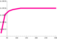
   a)      b)

Figure 1: a. $Z^{X}_{3}Z^{b,c}_{3}$ for D=10,    b. $Z^{X}_{3}Z^{b,c}_{3}$ for D=26

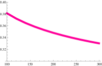
   a)        f)

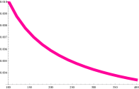
   b)        g)

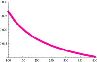
   c)     h)

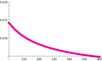
   d)     i)

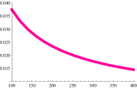
   e)     j)

Figure 2: $a)-e)$  Graphs show the effect of the different truncations in the calculation of the fermionic determinants $Z_{3}^{\psi}Z_{3}^{\beta\gamma}$; $f)-j)$  show dependence on $N$ of the total $\mathcal{Z}^{osc}_{3}$.

We see that the factorized form of the fermionic matrices produces less singular answers, but still the coefficients $\mathcal{Z}^{osc}_{3}$ diverge logarithmically.

 

6 Conclusion

We have checked descent relations $\langle V_{2}\mid V_{1}\rangle=\mathcal{Z}_{2}\langle V_{1}|$ and $\langle V_{3}\mid V_{1}\rangle=\mathcal{Z}_{3}\langle V_{2}|$ for NS sector of SSFT. We have performed calculations in the usual oscillator basis and in the $\kappa$ basis. We have found unexpected situation with the normalization factor $\mathcal{Z}_{3}$.

• First, our calculations show that starting from vertices subject to overlap relations we as a rule get nontrivial $\mathcal{Z}_{3}$

• Second, different schemes of calculations gives different $\mathcal{Z}_{3}$ and therefore $\mathcal{Z}_{3}$ has no universal meaning.

In both schemes of calculation used in the paper the vertex is factorized into the vertices of the bosonic and fermionic matter and their ghosts and we checked the descent relations separately for each vertex. These vertices have produced four coefficients $Z_{3}$. In the total descent relation we got the product of all these factors $\mathcal{Z}_{3}=Z^{X}Z^{bc}Z^{\psi}Z^{\beta\gamma}$.

We start our calculation in $\kappa$-basis. The regularized spectral density (4.2.2) has the divergent and finite parts. Due to the special tuning of the regularization the divergent parts of regularized spectral densities are the same for arbitrary conformal weights. Just due to this choice we have got the nonsingular $\mathcal{Z}_{3}^{\kappa}$. If one uses regularized spectral densities different from given in (4.2.2) one gets a different answer. For example, working with the same regularized spectral densities for fermionic and bosonic sectors we would get an other finite part for $\mathcal{Z}_{3}^{\kappa}$. Generally speaking using other regularization scheme one even cannot guarantee that $\mathcal{Z}_{3}$ will be finite. If we didn’t use the regularization of the inner product, we would probably get the divergent factor $\mathcal{Z}_{3}$ in the $\kappa$-basis. The level truncation method demonstrates also an appearance of divergencies. Namely, performing calculation of the descent relation in the discrete basis we got that the factor $\mathcal{Z}^{osc}_{3}$ logarithmically diverges. One can say that in the oscillation scheme the regularization using truncations of the infinite Neumann matrices by $N\times N$ matrices appears to be unlucky and brings divergencies for $\mathcal{Z}^{osc}_{3}$. It can happen that exist a special truncation method that provide a finite $Z_{3}$ in SSFT. Note that the truncation method used in [15] for the bosonic string give the $\mathcal{Z}^{x,bc}_{3}=1$.

Therefore, the different methods and schemes of the calculations produce the different regularizations. There are several papers [12, 13, 14, 15, 28] in which the factor $\mathcal{Z}_{3}=Z^{X}Z^{bc}$ was calculated in the bosonic string. Different methods of calculations have been used and different factors $\mathcal{Z}_{3}$ have been obtained. This is in agreement with our general discussion.

The same technique can be used to get descent relations in the alternative formulation of SSFT [43].

Appendix A Neumann matrices $V^{ab}$ and $I$

The Neumann matrices $V^{ab}$ and $I$ for the vertices $\langle V_{3}^{\psi}|$ and $|V_{1}^{\psi}\rangle$ have the form [29, 30]:

$$V^{aa}=\frac{F\tilde{F}}{(1-F)(2+F)},$$ (1a)

$$V^{aa+1}=\frac{\tilde{F}+iC(1-F)}{(1-F)(2+F)},$$ (1b)

$$V^{aa-1}=\frac{\tilde{F}-iC(1-F)}{(1-F)(2+F)},$$ (1c)

$$I=\frac{\tilde{F}}{1-F}=-\frac{1+F}{\tilde{F}}.$$ (1d)

Here the matrices $F$, $\tilde{F}$ and $C$ take the form [4]

$$F_{rs} = -\frac{2}{\pi}\frac{i^{r-s}}{r+s},\quad r=s\text{ mod}(2),$$

$$\tilde{F}_{rs} = \frac{2}{\pi}\frac{i^{r+s}}{s-r},\quad r=s+1\text{ mod}(2),$$ (2)

$$C_{rs} = (-1)^{r}\delta_{rs}.$$

with the following properties

$$F^{2}-\tilde{F}^{2}=1,\quad[F,\tilde{F}]=0,$$ (3)

$$CFC=-F,\quad F^{T}=F,\quad C\tilde{F}C=\tilde{F},\quad\tilde{F}^{T}=-\tilde{F}.$$

At first we evaluate the matrix $1-IV^{11}$:

$$1-IV^{11}=1+\frac{1+F}{\tilde{F}}\frac{F\tilde{F}}{(1-F)(2+F)}=\frac{2}{(1-F)(2+F)}.$$ (4)

Let us consider the diagonal elements of matrix $R^{pq}$:

$$R^{pp} = V^{pp}+V^{p1}\frac{1}{1-IV^{11}}IV^{1p}=$$

$$= \frac{F\tilde{F}}{(1-F)(2+F)}+\frac{\tilde{F}\mp iC(1-F)}{(1-F)(2+F)}\frac{(1-F)(2+F)}{2}\frac{\tilde{F}}{1-F}\frac{\tilde{F}\pm iC(1-F)}{(1-F)(2+F)}=$$

$$= \frac{F\tilde{F}}{(1-F)(2+F)}+\frac{1}{2}(\tilde{F}\mp iC(1-F))^{2}\frac{\tilde{F}}{(1-F)^{2}(2+F)}$$

$$= \frac{F\tilde{F}}{(1-F)(2+F)}+\frac{1}{2}(\tilde{F}^{2}-(1-F)^{2})\frac{\tilde{F}}{(1-F)^{2}(2+F)}=$$

$$= \frac{F\tilde{F}}{(1-F)(2+F)}-\frac{(1-F)F\tilde{F}}{(1-F)^{2}(2+F)}=0.$$

Next we evaluate the non-diagonal elements of $R^{pq}$:

$$R^{pp\pm 1} = V^{pp\pm 1}+V^{p1}\frac{1}{1-IV^{11}}IV^{1p\pm 1}=$$

$$= \frac{\tilde{F}\pm iC(1-F)}{(1-F)(2+F)}+\frac{\tilde{F}\mp iC(1-F)}{(1-F)(2+F)}\frac{(1-F)(2+F)}{2}\frac{\tilde{F}}{(1-F)}\frac{\tilde{F}\mp iC(1-F)}{(1-F)(2+F)}=$$

$$= \frac{\tilde{F}\pm iC(1-F)}{(1-F)(2+F)}-\frac{(1\mp i\tilde{F}C)\tilde{F}}{(1-F)(2+F)}=\pm\frac{iC(1-F-\tilde{F}^{2})}{(1-F)(2+F)}=\pm iC.$$

Appendix B Neumann matrices $K^{ab}$ and $\tilde{I}$

The Neumann matrices $K^{ab}$ and $\tilde{I}$ for the vertices $\langle V_{3}^{\beta\gamma}|$ and $|V_{1}^{\beta\gamma}\rangle$ have the form

$$K^{aa}=\frac{F\tilde{F}}{(1+F)(2-F)},$$ (5a)

$$K^{aa+1}=\frac{-\tilde{F}-iC(1+F)}{(1+F)(2-F)},$$ (5b)

$$K^{aa-1}=\frac{-\tilde{F}+iC(1+F)}{(1+F)(2-F)},$$ (5c)

$$\tilde{I}_{rs}=-\frac{\tilde{F}}{1+F}=\frac{1-F}{\tilde{F}}.$$ (5d)

Using the representation of the Neumann matrices (5) we can evaluate analytically $U^{pq}$ like in the case of the fermionic matter. At first we evaluate the inverse matrix $1-\tilde{I}K^{11}$:

$$1-\tilde{I}K^{11}=1-\frac{1-F}{\tilde{F}}\frac{F\tilde{F}}{(1+F)(2-F)}=\frac{2}{(1+F)(2-F)}.$$ (6)

Let us consider the diagonal elements of matrix the $U^{pq}$:

$$U^{pp} = K^{pp}+K^{p1}\frac{1}{1-\tilde{I}K^{11}}\tilde{I}K^{1p}=$$

$$= \frac{F\tilde{F}}{(1+F)(2-F)}+\frac{1}{2}(-\tilde{F}\pm iC(1+F))^{2}\frac{\tilde{F}}{(1+F)^{2}(2-F)}=$$

$$= \frac{F\tilde{F}}{(1+F)(2-F)}-\frac{(1+F)F\tilde{F}}{(1+F)^{2}(2-F)}=0.$$

Next we evaluate the non-diagonal elements of $U^{pq}$:

$$U^{pp\pm 1} = K^{pp\pm 1}+K^{p1}\frac{1}{1-\tilde{I}K^{11}}\tilde{I}K^{1p\pm 1}=$$

$$= \frac{-\tilde{F}\mp iC(1+F)}{(1+F)(2-F)}+\frac{(1\mp i\tilde{F}C)\tilde{F}}{(1+F)(2-F)}=\mp\frac{iC(1+F-\tilde{F}^{2})}{(1+F)(2-F)}=\mp iC.$$

References

- [1] E. Witten, Noncommutative Geometry and String Field Theory, Nucl. Phys. B268 253 (1986); E. Witten, Interacting Field Theory of Open Superstrings, Nucl.Phys. B276 291 (1986).
-
[2]
I. Ya. Arefeva, P. B. Medvedev and A. P. Zubarev,
Background Formalism For Superstring Field Theory, Phys. Lett.
B240 356 (1990);
I.Ya. Arefeva, P.B. Medvedev and A.P. Zubarev, NewRepresentation For String Field Solves The Consistency Problem For Open Superstring Field Theory, Nucl.Phys. B341 464 (1990). - [3] C. Preitschopf, C. Thorn and S. Yost, Superstring Field Theory, Nucl. Phys. B337 363 (1990).
- [4] D. Gross, A. Jevicki, Operator Formulation of Interacting String Field Theory (I), (II), Nucl.Phys. B283 1 (1987), B287 225 (1987), Operator Formulation of Interacting String Field Theory (III). NSR superstring, Nucl.Phys. B293 29 (1987).
- [5] A. LeClair, M. Peskin and C. Preitschopf, String Field Theory on the Conformal Plane (I). Kinematical Principles, Nucl. Phys. B317 411 (1989); String Field Theory on the Conformal Plane (II). Generalized Gluing, Nucl. Phys. B317 464 (1989).
-
[6]
E. Cremmer, A. Schwimmer and C. B. Thorn,
The Vertex Function in Witten s Formulation of String Field Theory,
Phys. Lett.
B179 57 (1986);
S. Samuel, The Physical and Ghost Vertices in Witten’s String Field Theory, Phys. Lett. B181 255 (1986);
N. Ohta, Covariant Interacting String Field Theory in the Fock-Space Representation , Phys. Rev. D34 3785 (1986). - [7] K. Ohmori, A review on tachyon condensation in open string field theories, hep-th/0102085.
- [8] I. Ya. Arefeva, D. M. Belov, A. A. Giryavets, A. S. Koshelev and P. B. Medvedev, Noncommutative Field Theories and (Super)String Field Theory, hep-th/0111208.
- [9] W. Taylor and B. Zwiebach, D-branes, tachyons, and string field theory, hep-th/0311017.
- [10] L. Bonora, C. Maccaferri, D. Mamone and M. Salizzoni, Topics in string field theory, hep-th/0304270.
- [11] W. Taylor, Perturbative Diagrams in String Field Theory [hep-th/0207132]; I. Ellwood, J. Shelton and W. Taylor, Tadpoles and closed string backgrounds in open string field theory, JHEP 0307, 059 (2003).
- [12] D. M. Belov, Witten’s ghost vertex made simple (bc and bosonized ghosts), Phys. Rev. D 69, 126001 (2004).
- [13] E. Fuchs and M. Kroyter, Normalization anomalies in level truncation calculations, JHEP 0512 031 (2005).
- [14] I. Ya. Aref’eva, R. Gorbachev, P. B. Medvedev and D. V. Rychkov, Descent relations and oscillator level truncation method, Theor. Math. Phys. 150, 2 (2007).
- [15] E. Fuchs and M. Kroyter, Universal regularization for string field theory, JHEP 0702, 038 (2007).
- [16] L. Rastelli, A. Sen and B. Zwiebach, Star algebra spectroscopy, JHEP 0203, 029 (2002).
- [17] D. Friedan, E. Martinec and S. Shenker, Conformal Invariance, Supersymmetry and String Theory, Nucl.Phys. B271 93 (1986); D. Friedan, Notes On String Theory And Two-Dimensional Conformal Field Theory, Published in S.Barbara Workshop:String 1985:0162.
- [18] I. Ya. Arefeva and P. B. Medvedev, Oscillator Representation for Picture Changing Operators, Theor. Math. Phys. 82 23 (1990).
- [19] D. Belov, Diagonal Representation Of Open String Star And Moyal Product [hep-th/0204164].
- [20] I. Bars, Map of Witten’s * to Moyal’s *, Phys. Lett. B517 436 (2001).
- [21] D. M. Belov and C. Lovelace, Star products made easy, Phys. Rev. D 68, 066003 (2003).
- [22] K. Okuyama, Ghost kinetic operator of vacuum string field theory, JHEP 0201, 027 (2002).
- [23] M. R. Douglas, H. Liu, G. W. Moore and B. Zwiebach, Open string star as a continuous Moyal product, JHEP 0204, 022 (2002)
- [24] D. Belov, Representation of Small Conformal Algebra in -basis [hep-th/0210199].
- [25] T. Erler, Moyal Formulation of Witten’s Star Product in the Fermionic Ghost Sector [hep-th/0205107].
- [26] B. Feng, Y. H. He and N. Moeller, The spectrum of the Neumann matrix with zero modes, JHEP 0204, 038 (2002).
- [27] D. M. Belov and A. Konechny, On continuous Moyal product structure in string field theory, JHEP 0210, 049 (2002); D. M. Belov and A. Konechny, On spectral density of Neumann matrices, Phys. Lett. B 558, 111 (2003).
- [28] E. Fuchs, M. Kroyter and A. Marcus, Virasoro operators in the continuous basis of string field theory, JHEP 0211, 046 (2002); E. Fuchs, M. Kroyter and A. Marcus, Continuous half-string representation of string field theory, JHEP 0311, 039 (2003).
- [29] I. Ya. Arefeva and A. A. Giryavets, Open superstring star as a continuous Moyal product, Russ. Phys. J. 45, 651 (2002).
- [30] M. Marino and R. Schiappa, Towards vacuum superstring field theory: The supersliver, J. Math. Phys. 44, 156 (2003).
- [31] T. G. Erler, A fresh look at midpoint singularities in the algebra of string fields, JHEP 0503 042 (2005).
- [32] L. Bonora, C. Maccaferri, R. J. Scherer Santos and D. D. Tolla, Ghost story. I. Wedge states in the oscillator formalism, JHEP 0709, 061 (2007).
- [33] C. Thorn, String Field Theory, Phys. Rept. 175 1 (1989).
- [34] L. Rastelli and B. Zwiebach, Tachyon potentials, star products and universality, JHEP 0109 038 (2001).
- [35] I. Ellwood, B. Feng, Y. H. He and N. Moeller, The identity string field and the tachyon vacuum, JHEP 0107 016 (2001).
- [36] I. Kishimoto and K. Ohmori, CFT description of identity string field: Toward derivation of the VSFT action, JHEP 0205, 036 (2002).
- [37] S. Samuel, Mathematical Formulation of E.Wittens Superstring Field Theory, Nucl. Phys. B296 187 (1988).
- [38] I. Ya. Arefeva, A. A. Giryavets and P. B. Medvedev, NS matter sliver, Phys. Lett. B 532, 291 (2002).
- [39] I. Ya. Arefeva, A. A. Giryavets and A. S. Koshelev, NS ghost slivers, Phys. Lett. B 536, 138 (2002).
- [40] W. Rühl, The Lorentz Group and Harmonic Analysis, Benjamin (1970), Ch. 5.
- [41] J. L. Manes, An Anomalous Transformation in String Field Theory, Nucl. Phys. B303 305 (1988).
- [42] R. Potting and C. Taylor, The Midpoint Transformation in Witten’s String Field Theory, Nucl. Phys. B316 59 (1989).
- [43] N. Berkovits, Super-Poincare Invariant Superstring Field Theory, Nucl. Phys. B450 90 (1995).