Flow instabilities of magnetic flux tubes

Abstract

Context. Flow-induced instabilities are relevant for the storage and dynamics of magnetic fields in stellar convection zones and possibly also in other astrophysical contexts.

Aims. We continue the study started in the first paper of this series by considering the stability properties of longitudinal flows along magnetic flux tubes.

Methods. A linear stability analysis was carried out to determine criteria for the onset of instability in the framework of the approximation of thin magnetic flux tubes.

Results. In the non-dissipative case, we find Kelvin-Helmholtz instability for flow velocities exceeding a critical speed that depends on the Alfvén speed and on the ratio of the internal and external densities. Inclusion of a friction term proportional to the relative transverse velocity leads to a friction-driven instability connected with backward (or negative energy) waves. We discuss the physical nature of this instability. In the case of a stratified external medium, the Kelvin-Helmholtz instability and the friction-driven instability can set in for flow speeds significantly lower than the Alfvén speed.

Conclusions. Dissipative effects can excite flow-driven instability below the thresholds for the Kelvin-Helmholtz and the undulatory (Parker-type) instabilities. This may be important for magnetic flux storage in stellar convection zones and for the stability of astrophysical jets.

1 Introduction

The stability of magnetic structures with field-aligned flows is of potential astrophysical relevance in relation to magnetic flux storage in stellar convection zones, for siphon flows and other flows in stellar atmospheres and envelopes, as well as for jets and collimated outflows. While the first paper of this series (Schüssler & Ferriz-Mas, 2007) studied the effects of perpendicular flows on the stability of magnetic flux tubes, here we consider the case of parallel flows, directed along the tube.

Linear stability properties of field-aligned flows in ideal MHD have been considered previously with regard to the Kelvin-Helmholtz instability by various authors (e.g., Chandrasekhar, 1961; Parker, 1964; Ray, 1981; Ferrari et al., 1981; Satya Narayanan & Somasundaram, 1982; Rae, 1983; D’Silva & Choudhuri, 1991; Cheng, 1994; Kolesnikov et al., 2004). Dissipative effects leading to instability in the presence of longitudinal (shear) flows, connected with the appearance of negative energy waves, have been discussed by Ryutova (1988, 1990) and Joarder et al. (1997) and, in connection with resonant absorption of waves in shear layers, by Hollweg et al. (1990), Goossens et al. (1992), Tirry et al. (1998), and Andries & Goossens (2001a, b).

The effect of a longitudinal flow along a thin toroidal magnetic flux tube has been considered by van Ballegooijen (1983) and Ferriz-Mas & Schüssler (1993, 1995) in the case of a rotating star and by Achterberg (1996b) in the case of a Keplerian accretion disk. A general formalism for the stability of stationary flows along curved thin magnetic flux tubes has been developed by Schmitt (1998).

The work presented here is motivated by the unexpected appearance of instabilities in numerical simulations of thin flux tubes in stellar convection zones (Holzwarth, 2002) in parameter domains where linear analysis predicts stability (e.g., Ferriz-Mas & Schüssler, 1995). The instabilities could be traced back to the aerodynamic drag force included in the simulations, which does not appear in linear analysis owing to its quadratic dependence on the relative velocity between flux tube and environment. Such instabilities affect the storage of magnetic flux at the bottom of a stellar convection zone, so that a systematic investigation of the underlying physical mechanisms and the consequences for flux storage is called for. Our study is carried out in the framework of the thin flux tube approximation (Spruit, 1981), which is relevant for magnetic structures in the deep layers of a stellar convection zone. This approximation is still the only possibility to carry out numerical simulations of the dynamics of magnetic structures in these layers with realistically high values of the plasma $\beta$ (ratio of gas pressure to magnetic pressure), since the correspondingly low density, temperature, and pressure contrasts are difficult to maintain against numerical diffusion in 2D/3D MHD simulations.

Of particular importance with respect to the question of flux storage is the inclusion of stratification effects, so that the combined effects of flow-driven instability and Parker instability can be studied. We provide a unified linear treatment of the Kelvin-Helmholtz instability, dissipative (friction-induced) instability, and the undulatory (Parker-type) instability in a gravitationally stratified medium. While we restrict ourselves here to straight flux tubes in a plane-parallel stratification in order to elucidate the physical mechanisms, the subsequent paper in the series will consider the case of toroidal flux tubes and will quantitatively discuss the relevance of these instabilities in rotating stars and the dependence on the stratification parameters, with particular attention to the problem of flux storage in stellar convection zones.

The paper is organized as follows. We first consider the stability of a straight flux tube with longitudinal flow in a (non-stratified) uniform background medium in Sect. 2. The treatment is extended in Sect. 3 to include the effect of gravitational stratification. Section 4 gives our conclusions.

2 Uniform background medium

As a first example, we consider a straight, untwisted magnetic flux tube, which harbors a flow along the field lines with constant velocity, $u_{0}$, and is embedded in a uniform and static environment. Under these circumstances, the equilibrium for a thin flux tube is simply given by the condition of total pressure balance,

$$p_{\rm e0}=p_{\rm i0}+{B_{0}^{2}\over 8\pi}\,,$$ (1)

where $p_{\rm e0}$ and $p_{\rm i0}$ are the gas pressures in the environment and within the flux tube, respectively, and $B_{0}={\rm const.}$ is the magnetic field strength. We indicate equilibrium quantities by an index “0”. Following previous work (e.g., Spruit & van Ballegooijen, 1982; Schüssler, 1990; Ferriz-Mas & Schüssler, 1993, 1995; Schmitt, 1998), we consider a Lagrangian displacement, $\@vec{\xi}$, of the equlibrium flux tube, expressed in terms of the Frenet basis, $\{\@vec{e}_{\rm t0},\@vec{e}_{\rm n0},\@vec{e}_{\rm b0}\}$ in the tangential, normal, and binormal directions of the equilibrium flux tube,

$$$$\@vec{\xi}=\xi_{\rm t}\@vec{e}_{\rm t0}+\xi_{\rm n}\@vec{e}_{\rm n0}+\xi_{\rm b}\@vec{e}_{\rm b0}\,.$$ (2)

We define the direction of $\@vec{e}_{\rm t0}$ such that $u_{0}\geq 0$. For a straight flux tube, $\@vec{e}_{\rm n0}$ and $\@vec{e}_{\rm b0}$ can be defined as any pair of orthogonal vectors that are perpendicular to $\@vec{e}_{\rm t0}$ such that $\{\@vec{e}_{\rm t0},\@vec{e}_{\rm n0},\@vec{e}_{\rm b0}\}$ forms a right-handed basis. The displacement components are functions of time, $t$, and arc length along the equilibrium flux tube, $s_{0}$.

2.1 Kelvin-Helmholtz instability

In the ideal case without friction between the flux tube and its surroundings (or other dissipative processes), a uniform, straight flux tube can only become unstable owing to the Kelvin-Helmholtz instability. The linearized equations for the three components of the displacement vector are all decoupled from each other. For a transverse displacement in the normal direction we have (see Schmitt, 1998)

$$\mu\ddot{\xi}_{\rm n}+2u_{0}\dot{\xi}^{\,\prime}_{\rm n}+(u_{0}^{2}-u_{\rm A}^{2}){\xi}^{\prime\prime}_{\rm n}=0\,,$$ (3)

where $u_{\rm A}=B_{0}/(4\pi\rho_{\rm i0})^{1/2}$ is the Alfvén velocity. Dots indicate (partial) time derivatives and primes denote derivatives with respect to arc length, $s_{0}$. The factor $\mu=1+(\rho_{\rm e0}/\rho_{\rm i0})$ takes into account the co-acceleration of the surrounding medium as a consequence of a transverse acceleration of the flux tube, leading to enhanced inertia (e.g., Spruit, 1981; Moreno-Insertis et al., 1996; Achterberg, 1996a). Here, $\rho_{\rm e0}$ and $\rho_{\rm i0}$ are the gas densities outside and inside the equilibrium flux tube, respectively. The corresponding equation for the binormal component of the displacement is analoguous to Eq. (3). The tangential component describes (Doppler-shifted) longitudinal tube waves, which are of no further interest in this context.

Inserting into Eq. (3) an exponential ansatz of the form $\xi_{\rm n}\propto\exp i(ks_{0}-\omega t)$, with real wavenumber $k\geq 0$ and complex frequency $\omega$, leads to the dispersion relation

$$\mu\omega^{2}-2u_{0}k\omega+k^{2}\left(u_{0}^{2}-u_{\rm A}^{2}\right)=0\,.$$ (4)

Instability, i.e., an exponentially growing mode, corresponds to a positive imaginary part of $\omega$. In the case $k=0$, Eq. (4) only has the trivial solution, while for $k\neq 0$ we have instability if the flow velocity surpasses a critical velocity, viz.

$$u_{0}>\left({\mu\over\mu-1}\right)^{1/2}u_{\rm A}\,.$$ (5)

Note that a finite value for the critical velocity requires that $\mu>1$, i.e., that the acceleration of the surrounding medium is taken into account. In order to identify the character of this instability, we compare the condition derived here with the result for a ‘thick’ flux tube obtained by Kolesnikov et al. (2004) for incompressible perturbations. In the thin-tube limit, $kR\ll 1$, where $R$ is the tube radius, the dispersion relation [their Eq. (27)] becomes identical to our Eq. (4), if we take into account the sign flip in their definition of $\omega$. Consequently, our analysis provides the thin-tube limit for the criterion for the Kelvin-Helmholtz instability. Furthermore, Kolesnikov et al. (2004) have shown that the critical velocity in the case of a thick tube becomes at most by about 10% higher than the value determined from Eq. (5), which therefore can be considered as a reasonable estimate (lower limit) for all flux tubes. Similar criteria have been given by Ryutova (1990) and also by Achterberg (1982) and by Osin et al. (1999), but the connection to the Kelvin-Helmholtz instability was not made in the latter two papers.

We have verified further (see Appendix A) that the result does not depend on the chosen frame of reference, i.e., whether one considers a flow within the flux tube with the exterior at rest or a (uniform) external flow along a static flux tube. This is obvious for the ‘thick’ flux tube treated by Kolesnikov et al. (2004), where the perturbation of the exterior is consistently taken into account, in contrast to the thin-tube case, where the effect of the exterior is solely described by the enhanced inertia term.

2.2 Friction-induced instability

Up to here, we have assumed the ideal case of a dissipationless plasma. Including dissipative processes can lead to qualitatively different behaviour. For magnetic flux tubes in stellar convection zones, the drag resulting from a motion of the tube perpendicular to its axis relative to the surrounding medium is an important dissipative process. For flows with large Reynolds number, the drag force is roughly proportional to the square of the relative perpendicular velocity (e.g., Parker, 1975; Batchelor, 1967, §5.11). In the case of a finite perpendicular velocity in the undisturbed flux tube equilibrium, a linear stability analysis has been carried out in the first paper of this series (Schüssler & Ferriz-Mas, 2007). In the case of a static background medium considered here, the drag force is of second order in the perturbations, so that its effect cannot be studied by way of a linear stability analysis. We therefore assume a Stokes-type friction, which is linear in the perpendicular velocity. It turns out that the resulting stability criteria are independent of the value of the proportionality factor (provided that it differs from zero) and we have reason to assume that the criteria are, in fact, independent of the nature of the dissipation process altogether. For instance, numerical thin-tube simulations including a quadratic drag force confirm the criteria derived under the assumption of a Stokes-type friction (see Holzwarth et al. in preparation, paper III of this series). We write the Stokes-type friction acceleration in the form

$${\@vec{a}}_{\rm S}=-\alpha\,({\@vec{u}}_{\rm rel}\cdot\@vec{e}_{\rm n})\,\@vec{e}_{\rm n0}$$ (6)

where $\alpha\geq 0$ is a constant parameter and

$${\@vec{u}}_{\rm rel}=\@vec{u}_{\rm i}-\@vec{u}_{\rm e}$$ (7)

is the relative velocity, i.e., the difference between the perturbed internal velocity, $\@vec{u}_{\rm i}$, and the external velocity, $\@vec{u}_{\rm e}$. Here we have $\@vec{u}_{\rm e}=\@vec{0}$ and thus obtain the linearized expression

$$\@vec{u}_{\rm rel} = u_{0}\@vec{e}_{\rm t0}+\dot{\@vec{\xi}}+u_{0}\@vec{\xi}^{\,\prime}$$ (8)

$$= (u_{0}+\dot{\xi}_{\rm t}+u_{0}\xi_{\rm t}^{\,\prime})\@vec{e}_{\rm t0}+(\dot{\xi}_{\rm n}+u_{0}\xi_{\rm n}^{\,\prime})\@vec{e}_{\rm n0}\,,$$ (9)

where

$$\@vec{e}_{\rm n}=\@vec{e}_{\rm n0}-\@vec{e}_{\rm t0}\xi_{\rm n}^{\,\prime}$$ (10)

is the perturbed unit normal vector. The linearized part of ${\@vec{a}}_{\rm S}$ provides an additional term of the form $\alpha\dot{\xi}_{\rm n}$ in Eq. (3), leading to a modification of the dispersion relation given by Eq. (4):

$$\mu\omega^{2}-2u_{0}k\omega+k^{2}\left(u_{0}^{2}-u_{\rm A}^{2}\right)+i\alpha\omega=0\,.$$ (11)

The resulting condition for instability (positive imaginary part of $\omega$) is simply given by

$$u_{0}>u_{\rm A}$$ (12)

for $k\neq 0$. Comparison with Eq. (5) shows that instability in the case with friction sets in for a lower critical velocity than for the Kelvin-Helmholtz instability, $u_{\rm KHI}=\sqrt{\mu/(\mu-1)}u_{\rm A}>u_{\rm A}$. This suggests that the effect of friction leads to a new kind of instability, which does not exist in the dissipationless case, although the condition for instability given by Eq. (12) is independent of the actual value of the friction parameter, as long as $\alpha$ does not vanish. In the limit $\alpha\to 0$, the growth rate of the friction-induced instability in the velocity range $u_{\rm A}<u_{0}<u_{\rm KHI}$ goes to zero, while for $u_{0}>u_{\rm KHI}$ we have Kelvin-Helmholtz instability. The criterion Eq. (12) is also independent of the enhanced-inertia parameter, $\mu$, which indicates that the instability mechanism is not closely related to the perturbation of the external medium, such as in the case of the Kelvin-Helmholtz instability.

In order to elucidate the nature of the friction-induced instability, we consider the phase velocity, $u_{\rm ph}={\rm Re}(\omega/k)$, of the unstable mode. It is readily shown that this mode has $u_{\rm ph}\geq 0$ for $u_{0}^{2}\geq u_{\rm A}^{2}$, so that the unstable mode is prograde, i.e., it propagates in the direction of the flow. For flow velocities below the instability limit, the direction of propagation of this mode is retrograde, against the flow. Modes whose direction of propagation becomes reversed by the flow are sometimes called backward waves (e.g., Nakariakov & Roberts, 1995; Joarder et al., 1997). The reversal of the propagation direction at the instability threshold means that both real and imaginary parts of $\omega$ change sign when $u_{0}-u_{\rm A}$ goes through zero. We see from Eq. (11) that this corresponds also to a sign change of the friction-related term, $i\alpha\omega$, in the dispersion relation: the effect of friction changes from wave damping to wave excitation.

Backward waves can also be negative energy waves (e.g., Cairns, 1979; Lashmore-Davies, 2005), which owe their name to the fact that they can grow in amplitude when the total kinetic energy of the system (energy of the flow plus that of the wave) is decreased (e.g., by some dissipative process). Following Cairns (1979), we call a given mode a negative energy wave if the relation

$$C\equiv\omega{\partial D\over\partial\omega}<0$$ (13)

holds, where $D$ represents the left-hand side of the dispersion relation in the non-dissipative case, here given by Eq. (4). In general, $D$ has to be multiplied by a factor $\pm 1$ such that $C>0$ in the case of a system without flows ($u_{0}=0$). In our case, the condition for negative energy waves becomes

$$\omega\left(\omega-{u_{0}k\over\mu}\right)<0\,.$$ (14)

Considering the solutions of Eq. (4),

$$\omega_{\pm}={u_{0}k\over\mu}\pm{u_{0}k\over\mu}\left(1-\mu+{\mu u_{\rm A}^{2}\over u_{0}^{2}}\right)^{1/2}\,,$$ (15)

we find that $\omega_{+}$ (the prograde mode) never satisfies the condition given by Eq. (14) while $\omega_{-}$ (the retrograde mode) in fact represents a negative energy wave provided that $u_{0}^{2}>u_{\rm A}^{2}$. Consequently, we find that the following three statements are all equivalent in our case: (1) we have friction-induced instability; (2) the system supports a backward wave mode; and (3) the system has a negative energy wave. The fact that our unstable mode is a negative energy wave suggests that not only the exact value of the friction coefficient is irrelevant for the stability criterion but that even the nature of the dissipation process is largely irrelevant. In fact, it has been shown that energy loss by radiation of MHD waves (Ryutova, 1988), thermal conduction (Joarder et al., 1997), or resonant absorption (Tirry et al., 1998) can provide the necessary dissipation for the development of the instability. On the other hand, the fact that Eq. (13) is not invariant with respect to Galilei transformations raises questions concerning the general validity of the concept of negative energy waves (e.g., Walker, 2000; Andries & Goossens, 2002), so that we do not pursue this approach any further.

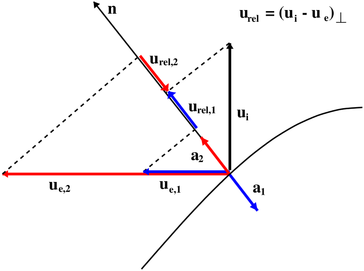
Figure 1: Schematic sketch illustrating the physical mechanism of the friction-driven flux tube instability. A leftward propagating transverse wave along the flux tube (indicated by the curved line) is amplified if the speed of the leftward external flow (in the frame of reference where the plasma in the equilibrium flux tube is at rest) exceeds the phase velocity of the wave. See main text for a detailed discussion.

The physical mechanism driving the friction-induced instability can be most easily understood by considering the frame of reference in which the plasma in the equilibrium flux tube is at rest. We then have an external flow along the equilibrium flux tube with a velocity $\@vec{u}_{\rm e}=-u_{0}\@vec{e}_{\rm t0}$. Figure 1 schematically shows a snapshot of a segment of the perturbed flux tube (black curve), together with velocity and acceleration vectors relevant for the effect of friction. We assume a transverse wave propagating leftward, i.e., in the direction of the external flow. The velocity $\@vec{u}_{\rm i}$ of a mass element of the tube corresponding to that wave motion is vertically upward for the tube segment and phase shown. The relative velocity between the tube and its environment that is relevant for the friction is given by the component of the velocity difference, $\@vec{u}_{\rm i}-\@vec{u}_{\rm e}$, along the instantaneous unit normal vector of the mass element, $\@vec{n}$, cf. Eqs. (6) and (7). Depending on the speed of the external flow, this projection can be parallel or antiparallel to the normal vector. We consider two cases: 1) for a sufficiently slow flow ($\@vec{u}_{\rm e,1}$, blue vector arrows in Fig. 1), the relative velocity ($\@vec{u}_{\rm rel,1}$) is parallel to the normal direction, so that the acceleration by friction ($\@vec{a}_{1}$) is antiparallel to the normal and thus decelerates the upward motion of the mass element, corresponding to a damping of the wave; 2) in the case of a sufficiently fast flow ($\@vec{u}_{\rm e,2}$, red vector arrows), the relative velocity ($\@vec{u}_{\rm rel,2}$) becomes antiparallel to the normal direction, so that the corresponding friction acceleration ($\@vec{a}_{1}$) is now parallel to the normal and accelerates the upward motion of the mass element, thus amplifying the wave. For a wave propagating to the right (reverse direction of $\@vec{u}_{\rm i}$), we always obtain damping.

We can put this in quantitative terms by considering the relative velocity,

$$u_{\rm rel}=(\@vec{u}_{\rm i}-\@vec{u}_{\rm e})\cdot\@vec{e}_{\rm n}=\dot{\xi}_{\rm n}-u_{0}\xi_{\rm n}^{\,\prime}\,.$$ (16)

Inserting a wave solution ${\xi}_{\rm n}\propto\sin(ks_{0}-\omega t)$, we readily find

$$u_{\rm rel}=(u_{\rm ph}+u_{0})u_{\rm ph}^{-1}\dot{\xi}_{\rm n}\,,$$ (17)

where $u_{\rm ph}=\omega/k$ is the phase velocity of the wave. Now, for $u_{\rm ph}>0$ the relative velocity has always the same sign as $\dot{\xi}_{\rm n}$, so that the wave is damped by friction. The same is true for $u_{\rm ph}<0$ and $u_{0}<-u_{\rm ph}$, while for $u_{0}>-u_{\rm ph}$ the sign of the factor in front of $\dot{\xi}_{\rm n}$ in Eq. (17) reverses, so that the friction force excites the wave. Figuratively, one can imagine the wave being amplified by a ‘tailwind’.

In the frame of reference with the external medium at rest, the condition $u_{0}>-u_{\rm ph}$ transforms into that for the ‘backward wave’, $u_{\rm ph}>0$.

3 Stratified background medium

We now consider the effect of a gravitational stratification of the external medium, so that buoyancy-driven instability (Spruit & van Ballegooijen, 1982; Ferriz-Mas & Schüssler, 1993, 1995) is included. For a straight, horizontal flux tube, mechanical equilibrium then requires neutral buoyancy, i.e., $\rho_{\rm i0}=\rho_{\rm e0}$, in addition to the pressure balance condition given by Eq. (1). We define the normal direction of the equilibrium flux tube to be along the (constant) gravitational acceleration. The linearized evolution of the three components of the displacement vector is then governed by the following system of equations:

$$\ddot{\xi}_{\scriptstyle\mathrm{t}}+2u_{0}\dot{\xi}_{\scriptstyle\mathrm{t}}^{\prime}+\left(u_{0}^{2}-u_{\scriptstyle\mathrm{A}}^{2}\right)\xi_{\scriptstyle\mathrm{t}}^{\prime\prime}-\frac{u_{\scriptstyle\mathrm{A}}^{2}}{\gamma H_{p}}\xi_{\scriptstyle\mathrm{n}}^{\prime}=0\,,$$ (18)

$$\mu\ddot{\xi}_{\scriptstyle\mathrm{n}}+2u_{0}\dot{\xi}_{\scriptstyle\mathrm{n}}^{\prime}+\left(u_{0}^{2}-u_{\scriptstyle\mathrm{A}}^{2}\right)\xi_{\scriptstyle\mathrm{n}}^{\prime\prime}+\alpha\dot{\xi}_{\scriptstyle\mathrm{n}}+\frac{u_{\scriptstyle\mathrm{A}}^{2}}{\gamma H_{p}}\xi_{\scriptstyle\mathrm{t}}^{\prime}+\omega_{\rm MBV}^{2}\xi_{\scriptstyle\mathrm{n}}=0\,,$$ (19)

$$\mu\ddot{\xi}_{\scriptstyle\mathrm{b}}+2u_{0}\dot{\xi}_{\scriptstyle\mathrm{b}}^{\prime}+\left(u_{0}^{2}-u_{\scriptstyle\mathrm{A}}^{2}\right)\xi_{\scriptstyle\mathrm{b}}^{\prime\prime}+\alpha\dot{\xi}_{\scriptstyle\mathrm{b}}=0\,.$$ (20)

In deriving these equations (see also Schmitt, 1998), we have assumed an ideal gas, adiabatic perturbations, and we have taken the limit $\beta=8\pi p_{0}/B_{0}^{2}\gg 1$, which reflects the conditions in stellar interiors. This simplifies the expressions without changing the character of the various instabilities. In Eqs. (18)-(20), $\gamma$ denotes the ratio of the specific heats, $H_{p}$ is the pressure scale height, $\alpha$ the friction parameter, and $\omega_{\rm MBV}$ is the magnetic Brunt-Väisälä frequency (cf. Moreno-Insertis et al., 1992) with

$$\omega_{\rm MBV}^{2}=\frac{u_{\scriptstyle\mathrm{A}}^{2}}{2H_{p}^{2}}\left[\frac{2}{\gamma}\left(\frac{1}{\gamma}-\frac{1}{2}\right)-\beta\delta\right]\,,$$ (21)

where $\delta=\nabla-\nabla_{\scriptstyle\mathrm{ad}}$ is the superadiabaticity of the external stratification. For $k=\alpha=0$ and $\omega_{\rm MBV}^{2}>0$, the perturbed flux tube would perform stable oscillations in the normal direction with $\omega=\omega_{\rm MBV}$. For $k=0$, $\omega_{\rm MBV}^{2}>0$, and $\alpha\neq 0$, the tube behaves like a damped harmonic oscillator. The binormal component, Eq. (20), is decoupled from the rest of the system and formally identical to the non-stratified case treated in the preceding section, so that the same results apply.

For the coupled normal and tangential components we again use an exponential ansatz of the form $\xi_{\rm t,n}(s_{0},t)=\hat{\xi}_{\rm t,n}\exp(iks_{0}-i\omega t)$ and normalize all frequencies by $ku_{\scriptstyle\mathrm{A}}$, writing $\tilde{\omega}=\omega/(ku_{\scriptstyle\mathrm{A}})$, $\tilde{\omega}_{\rm MBV}=\omega_{\rm MBV}/(ku_{\scriptstyle\mathrm{A}})$, and $\tilde{\alpha}=\alpha/(ku_{\scriptstyle\mathrm{A}})$. Inserting this into Eqs. (18) and (19) and keeping the same symbols for the non-dimensionalized quantities, we obtain the linear system

$$\left[\tilde{\omega}^{2}-2M_{\scriptstyle\mathrm{A}}\tilde{\omega}+\left(M_{\scriptstyle\mathrm{A}}^{2}-1\right)\right]\hat{\xi}_{\scriptstyle\mathrm{t}}+iq\hat{\xi}_{\scriptstyle\mathrm{n}}=0$$ (22)

$$\left[\mu\tilde{\omega}^{2}-2M_{\scriptstyle\mathrm{A}}\tilde{\omega}+\left(M_{\scriptstyle\mathrm{A}}^{2}-1\right)+i\tilde{\alpha}\tilde{\omega}-\tilde{\omega}_{\rm MBV}^{2}\right]\hat{\xi}_{\scriptstyle\mathrm{n}}-iq\hat{\xi}_{\scriptstyle\mathrm{t}}=0\,,$$ (23)

where $q\equiv 1/(\gamma H_{p}k)$ is a non-dimensional measure of the wavelength and $M_{\scriptstyle\mathrm{A}}\equiv u_{0}/u_{\scriptstyle\mathrm{A}}$ is the Alfvénic Mach number. This leads to a dispersion relation of the form

$$\mu\tilde{\omega}^{4}+c_{3}\tilde{\omega}^{3}+c_{2}\tilde{\omega}^{2}+c_{1}\tilde{\omega}+c_{0}=0$$ (24)

with

$$c_{3} = -2(\mu+1)M_{\scriptstyle\mathrm{A}}+i\tilde{\alpha}\,,$$ (25)

$$c_{2} = (\mu+1)\left(M_{\scriptstyle\mathrm{A}}^{2}-1\right)+4M_{\scriptstyle\mathrm{A}}^{2}-\tilde{\omega}_{\rm MBV}^{2}-2iM_{\scriptstyle\mathrm{A}}\tilde{\alpha}\,,$$ (26)

$$c_{1} = 2M_{\scriptstyle\mathrm{A}}\tilde{\omega}_{\rm MBV}^{2}-\left(M_{\scriptstyle\mathrm{A}}^{2}-1\right)\bigl{(}4M_{\scriptstyle\mathrm{A}}-i\tilde{\alpha}\bigr{)}\,,$$ (27)

$$c_{0} = \left(M_{\scriptstyle\mathrm{A}}^{2}-1\right)\left(M_{\scriptstyle\mathrm{A}}^{2}-1-\tilde{\omega}_{\rm MBV}^{2}\right)-q^{2}\,.$$ (28)

3.1 Parker instability $(\mu=1,\,\tilde{\alpha}=0)$

In the case $\mu=1$ and $\tilde{\alpha}=0$, the transformation $\tilde{\omega}\to\tilde{\omega}-M_{\scriptstyle\mathrm{A}}$ leads to a simple biquadratic equation (Schmitt, 1998). The solutions show that the flow does not affect the stability properties in this case. The criterion for instability (positive imaginary part of $\tilde{\omega}$) is given by

$$\tilde{\omega}_{\rm MBV}^{2}<q^{2}-1\,,$$ (29)

which corresponds to the result of Spruit & van Ballegooijen (1982). The condition marks the onset of the buoyancy-driven undular instability or Parker instability. In fact, the stability criterion for the Parker instability remains unchanged for $\mu>1$. Note that, owing to our chosen non-dimensionalisation, the wavelength-dependence of the Parker instability is hidden in $\tilde{\omega}_{\rm MBV}={\omega}_{\rm MBV}/(ku_{\rm A})$ and $q=1/(\gamma H_{p}k)$.

Figure 2: Kelvin-Helmholtz instability in the case with external stratification ($\mu=2$, $q=1$, $\tilde{\omega}_{\rm MBV}^{2}=0.2$) without friction ($\tilde{\alpha}=0$). The full and dashed lines give the real and imaginary parts, respectively, of the (normalized) frequency, $\tilde{\omega}$, for the four solutions of the dispersion relation, Eq. (24), as functions of the Alfvénic Mach number of the longitudinal flow, $M_{\scriptstyle\mathrm{A}}$. Instability sets in for $M_{\scriptstyle\mathrm{A}}\simeq 0.55$, when the real parts of the two (mainly) transverse modes merge and the imaginary part of $\tilde{\omega}$ becomes positive for one of the modes. The two modes whose real parts cross the zero line at $M_{\scriptstyle\mathrm{A}}\simeq 0.31$ and $M_{\scriptstyle\mathrm{A}}\simeq 1.45$, respectively, represent backward modes. They become unstable if friction is included $(\tilde{\alpha}>0)$.

Figure 3: Critical Alfvénic Mach numbers for the onset of the friction-induced instability as a function of the non-dimensionalized wavelength, $q$, for $\tilde{\omega}_{\rm MBV}^{2}=0.2$. For one of the two modes that can become unstable backward waves, the critical Mach number goes to zero as the wavelength approaches the value for the onset of the Parker instability, $q=(1+\tilde{\omega}_{\rm MBV}^{2})^{1/2}$ (indicated by the dashed vertical line). The dotted line indicates the case $q=1$ shown in Fig. 2.

Figure 4: Kelvin-Helmholtz and friction-induced instability for the same case as that shown in Fig. 2, now with $\tilde{\alpha}=0.2$. The real and imaginary parts of the normalized frequency, $\tilde{\omega}$, are given by the full and dashed lines, respectively. The upper panel shows all four modes and the full range of frequencies, while the lower panel gives a detail of the zero crossing of the two backward modes.

3.2 Kelvin-Helmholtz instability $(\mu>1,\,\tilde{\alpha}=0)$

For $\mu>1$, we have the possibility of a Kelvin-Helmholtz instability (cf. Sect. 2.1), now modified by the presence of stratification. If the flux tube is stable with respect to the Parker instability, i.e., if the instability condition given by Eq. (29) is not met, Kelvin-Helmholtz instability sets in for a flow exceeding a critical Alfvénic Mach number, $M_{\scriptstyle\mathrm{A,c}}$, which varies between zero for neutral Parker instability (i.e., $\tilde{\omega}_{\rm MBV}^{2}=q^{2}-1$) and infinity for $\tilde{\omega}_{\rm MBV}^{2}\to\infty$. Hence, a flux tube equilibrium approaching the stability limit of the Parker instability may become Kelvin-Helmholtz unstable for arbitrarily low Alfvénic Mach number.

The physical reason for this behavior is the fact that near the stability limit for the Parker instability, most of the stabilizing effect of the magnetic tension force has already been compensated for by the stratification effects, so that a low flow velocity is sufficient to destabilize the system. As an example, Fig. 2 shows the real and imaginary parts of the complex frequency, $\tilde{\omega}$, as a function of $M_{\scriptstyle\mathrm{A}}$ for $\mu=2$, $q=1$, $\tilde{\alpha}=0$, and $\tilde{\omega}_{\rm MBV}^{2}=0.2$. In the limit $H_{p}\to\infty$ ($q\to 0$, ${\omega}_{\rm MBV}\to 0$, non-stratified case), the two mode pairs represent the transverse and longitudinal tube modes (Spruit, 1981). With stratification, longitudinal and transverse perturbations are coupled and the modes are of a mixed type. Kelvin-Helmholtz instability sets in at $M_{\scriptstyle\mathrm{A}}\simeq 0.55$, when the real parts of the frequencies of one pair (corresponding to the transverse mode in the unstratified case) merge and an unstable mode (positive imaginary part) appears. In the non-stratified case, the critical Alfvénic Mach number is significantly larger, namely equal to $\sqrt{2}$ [cf. Eq. (5)].

3.3 Friction-induced instability $(\tilde{\alpha}\neq 0)$

In the case $\tilde{\alpha}>0$, the effect of friction adds another possibility for instability. Guided by the results discussed in Sect. 2.2, we conjecture that the instability is connected with backward waves, leading to a reversal of the sign of the friction term in Eq. (23). This conjecture is verified by direct numerical solution of the dispersion relation, Eq. (24). Fig. 2 shows that the real part of the frequency for two modes goes from negative to positive sign, indicating the presence of two backward waves for suffienctly high values of $M_{\scriptstyle\mathrm{A}}$. Writing $\tilde{\omega}=(\tilde{\omega}_{\scriptstyle\mathrm{r}},\tilde{\omega}_{\scriptstyle\mathrm{i}})$, the conditions for the presence of a backward wave becoming marginally unstable for $\tilde{\omega}=(0,0)$ are

$$\left.\frac{\mathrm{d}\tilde{\omega}_{\scriptstyle\mathrm{r}}}{\mathrm{d}M_{\scriptstyle\mathrm{A}}}\right|_{\tilde{\omega}=(0,0)}>0$$ (30)

and

$$\left.\frac{\mathrm{d}\tilde{\omega}_{\scriptstyle\mathrm{i}}}{\mathrm{d}M_{\scriptstyle\mathrm{A}}}\right|_{\tilde{\omega}=(0,0)}>0\,.$$ (31)

The dispersion relation, Eq. 24, shows that $\tilde{\omega}=(0,0)$ is equivalent to $c_{0}=0$, which entails the relation

$$\tilde{\omega}_{\rm MBV}^{2}\left(1-M_{\scriptstyle\mathrm{A}}^{2}\right)=q^{2}-\left(1-M_{\scriptstyle\mathrm{A}}^{2}\right)^{2}\,.$$ (32)

Taking the derivative of Eq. (24) with respect to $M_{\scriptstyle\mathrm{A}}$ and setting $\tilde{\omega}=(0,0)$ gives

$$c_{1}\left.\frac{\mathrm{d}\tilde{\omega}}{\mathrm{d}M_{\scriptstyle\mathrm{A}}}\right|_{\tilde{\omega}=(0,0)}+\frac{\mathrm{d}c_{0}}{\mathrm{d}M_{\scriptstyle\mathrm{A}}}=0\,.$$ (33)

Separating this equation into its real and imaginary parts leads to

$$\left.\frac{\mathrm{d}\tilde{\omega}_{\scriptstyle\mathrm{r}}}{\mathrm{d}M_{\scriptstyle\mathrm{A}}}\right|_{\tilde{\omega}=(0,0)}=\left(-\frac{\mathrm{d}c_{0}}{\mathrm{d}M_{\scriptstyle\mathrm{A}}}\frac{c_{\scriptstyle\mathrm{1,r}}}{c_{\scriptstyle\mathrm{1,r}}^{2}+c_{\scriptstyle\mathrm{1,i}}^{2}}\right),$$ (34)

and

$$\left.\frac{\mathrm{d}\tilde{\omega}_{\scriptstyle\mathrm{i}}}{\mathrm{d}M_{\scriptstyle\mathrm{A}}}\right|_{\tilde{\omega}=(0,0)}=-\frac{c_{\scriptstyle\mathrm{1,i}}}{c_{\scriptstyle\mathrm{1,r}}}\left.\frac{\mathrm{d}\tilde{\omega}_{\scriptstyle\mathrm{r}}}{\mathrm{d}M_{\scriptstyle\mathrm{A}}}\right|_{\tilde{\omega}=(0,0)}$$ (35)

where $c_{1}=(c_{\scriptstyle\mathrm{1,r}},c_{\scriptstyle\mathrm{1,i}})$ and $c_{0}$ is real. Inserting the expressions for these coefficients given in Eqs. (27) and (28) into Eq. (34) leads to a quadratic expression, which is positive as long as $M_{\scriptstyle\mathrm{A}}\neq 0$. Similarly, by using Eq. (27) and the relation given by Eq. (32), one shows that $-c_{\scriptstyle\mathrm{1,i}}/c_{\scriptstyle\mathrm{1,r}}>0$, so that both conditions for unstable backward waves given by Eqs. (30) and (31) are fulfilled. This extends our previous result that friction-induced instability occurs in the form of unstable backward waves to the case of a stratified medium.

The two mode pairs described by the dispersion relation Eq. (24) result from the combined action of the restoring forces of buoyancy (magnetic Brunt-Väisälä mode) and magnetic tension (transverse tube mode) in the system. In both cases, the retrograde member of the mode pair can become a backward wave, so that we expect two modes to become friction-unstable.

In fact, as already indicated in Fig. 2, each of the mode pairs resulting from the dispersion relation Eq. (24) exhibits a backward wave, becoming unstable at the critical Alfvénic Mach numbers given by the two roots of Eq. (32):

$$M_{\scriptstyle\mathrm{A,\pm}}^{2}=1+\frac{\tilde{\omega}_{\rm MBV}^{2}}{2}\left[1\pm\left(1+\frac{4q^{2}}{\tilde{\omega}_{\rm MBV}^{4}}\right)^{1/2}\right].$$ (36)

Note that, as long as they do not vanish, neither the value of $\tilde{\alpha}$ nor that of the enhanced interia factor, $\mu$, affect the stability criteria. It is only the growth rate of the unstable modes that depends on the value of $\tilde{\alpha}$.

Figure 3 shows the two branches of critical Alfvénic Mach numbers resulting from Eq. (36) for $\tilde{\omega}_{\rm MBV}^{2}=0.2$ as a function of the non-dimensionalized wavelength, $q$. For $q\to 0$, i.e. wavelength much smaller than the scale height, the lower branch corresponds to the result for the non-stratified case (transverse mode) with $M_{\scriptstyle\mathrm{A,-}}\to 1$, while the upper branch originates from the longitudinal tube mode. For finite wavelength, the upper branch goes to larger critical $M_{\scriptstyle\mathrm{A}}$, while the values decrease for growing $q$ in the lower branch. At the threshold for the onset of the Parker instability, $q=(1+\tilde{\omega}_{\rm MBV}^{2})^{1/2}$ (indicated by the dashed vertical line in Fig. 3), $M_{\scriptstyle\mathrm{A,-}}\to 0$. Similar to the case of the Kelvin-Helmholtz instability discussed in the previous subsection, a growing part of the stabilizing effect of the curvature force is compensated by buoyancy effects as the wavelength approaches the critical wavelength for the Parker instability, so that lower flow speeds suffice to trigger the friction-induced instability. The dotted vertical line in Fig. 3 indicates the case $q=1$ shown in Fig. 2: the intersections of this line with the two branches give the Mach numbers at which the corresponding two modes become backward waves (i.e., where the real part of $\tilde{\omega}$ changes its sign).

Fig. 4 shows the mode frequencies as a function of $M_{\scriptstyle\mathrm{A}}$ for $\mu=2$, $q=1$, $\tilde{\omega}_{\rm MBV}^{2}=0.2$ (same as for the case shown in Fig. 2), but now with a finite friction parameter: $\tilde{\alpha}=0.2$. The upper panel gives the mode structure in the same format as Fig. 2. The presence of friction removes the symmetry of the imaginary parts of $\tilde{\omega}$ (the growth rates) and also prohibits the mode merging at $M_{\scriptstyle\mathrm{A}}\simeq 0.55$ at the onset of the Kelvin-Helmholtz instability for $\tilde{\alpha}=0$. As shown in detail in the lower panel of Fig. 4, the first backward mode becomes unstable for $M_{\scriptstyle\mathrm{A}}\simeq 0.31$ and its the growth rate shows a significant upturn for $M_{\scriptstyle\mathrm{A}}\ga 0.55$, at which value the Kelvin-Helmholtz instability set in for $\tilde{\alpha}=0$. The second backward mode becomes unstable at $M_{\scriptstyle\mathrm{A}}\simeq 1.45$, but the system is by then already dominated by the first unstable mode. We note that, like in the unstratified case, the friction-induced instability sets in earlier (i.e., for lower values of $M_{\scriptstyle\mathrm{A}}$) then the Kelvin-Helmholtz instability.

4 Conclusions

In the framework of the approximation of thin flux tubes, we have provided a unified linear treatment of the Kelvin-Helmholtz instability, the dissipative (friction-induced) instability, and the undulatory (Parker-type) instability of a magnetic flux tube with a field-aligned flow in a gravitationally stratified medium. Including dissipation effects by a Stokes-like friction term leads to overstability of transverse waves for flow velocities below the threshold of the Kelvin-Helmholtz instability. In the case of a stratified medium, the critical flow velocity can become arbitrarily low near the threshold for Parker instability. In other words, for a given flow velocity, there is always a range of parameters (e.g., perturbation wavelength) that already give friction-induced instability before the Parker-type instability sets in.

The existence of friction-induced instability (overstability of transverse waves) potentially has important consequences for magnetic flux storage in stellar convection zones. Toroidal magnetic flux tubes require faster internal rotation (equivalent to a longitudinal flow) in order to keep force equilibrium (Moreno-Insertis et al., 1992). Although this flow is always sub-Alfvénic, we have seen that it still can lead to instability in a stratified medium. This will be studied in detail in the third paper of this series.

To include the drag-induced dissipation in our linear analysis, we have replaced the aerodynamic drag term (quadratic in the transverse velocity) commonly used in treatments of thin flux tubes by a Stokes-like friction term. As we will show by numerical simulations in paper III, this does not affect the stability criteria for the friction-induced instability derived here. In fact, the precise nature of the dissipation process is not crucial for the onset of the overstability associated with backward or negative-energy waves (cf., Joarder et al., 1997; Tirry et al., 1998).

Appendix A Kelvin-Helmholtz instability for external flow

The results of the stability analysis have to be independent of Galilean transformations of the frame of reference. Since, in our case, the effect of the external medium on the flux tube is described solely by the enhanced inertia for transverse acceleration (apart from the pressure balance condition), it is not completely straightforward to show that the result is Galilei invariant. Therefore, we give the derivation in what follows.

Assume a static straight equilibrium flux tube embedded in an external flow along the tube with $\@vec{u}_{\rm e}=\varv_{0}\@vec{e}_{\rm t0}$. Consider a displacement, $\xi_{\rm n}(s_{0},t)$, of a Langrangean mass element in the tube with normal acceleration $\ddot{\xi}_{\rm n}(s_{0},t)$. The corresponding acceleration of a mass element outside the flux tube is given by

$$\frac{\rm d}{{\rm d}t}\left[\frac{{\rm d}\xi_{\rm n}}{{\rm d}t}\right] = \frac{\rm d}{{\rm d}t}\left[\dot{\xi}_{\rm n}+\varv_{0}\xi_{\rm n}^{\prime}\right]$$ (37)

$$= \ddot{\xi}_{\rm n}+2\varv_{0}\xi_{\rm n}^{\prime}+\varv_{0}^{2}\xi_{\rm n}^{\prime\prime}\,,$$

where

$$\frac{\rm d}{{\rm d}t}=\frac{\partial}{{\partial}t}+\varv_{0}\frac{\partial}{{\partial}s_{0}}\,.$$ (38)

Dots indicate partial time derivatives and primes indicate partial derivatives with respect to arc length along the undisturbed tube. By using Eq. (37) and applying “actio = reactio”, we find for the normal component of the linearized equation of motion

$$\rho_{\rm i0}\ddot{\xi}_{\rm n}-\rho_{\rm i0}u_{\rm A}^{2}\xi_{\rm n}^{\prime\prime}=-\rho_{\rm e0}\left(\ddot{\xi}_{\rm n}+2\varv_{0}\xi_{\rm n}^{\prime}+\varv_{0}^{2}\xi_{\rm n}^{\prime\prime}\right).$$ (39)

Introducing $\mu=1+\rho_{\rm e0}/\rho_{\rm i0}$ and the ansatz $\xi_{\rm n}\propto\exp(iks_{0}-i\hat{\omega}t)$ into this equation, we obtain

$$\mu\hat{\omega}^{2}+(\mu-1)\left(k^{2}\varv_{0}^{2}-2\varv_{0}k\hat{\omega}\right)-k^{2}u_{\rm A}^{2}=0\,.$$ (40)

We now carry out a Galilean transformation into the rest frame of the external medium. In this frame of reference, we have an internal longitudinal flow with velocity $u_{0}\@vec{e}_{\rm t0}=-\varv_{0}\@vec{e}_{\rm t0}$. Inserting $u_{0}=-\varv_{0}$ and the transformation $\omega=\hat{\omega}-\varv_{0}k=\hat{\omega}+u_{0}k$ into Eq. (40), we find

$$\mu\omega^{2}-2u_{0}k\omega+k^{2}\left(u_{0}^{2}-u_{\rm A}^{2}\right)=0\,,$$ (41)

which is identical to Eq. (4).

References

- Achterberg (1982) Achterberg, A. 1982, A&A, 114, 233
- Achterberg (1996a) Achterberg, A. 1996a, A&A, 313, 1008
- Achterberg (1996b) Achterberg, A. 1996b, A&A, 313, 1016
- Andries & Goossens (2001a) Andries, J. & Goossens, M. 2001a, A&A, 368, 1083
- Andries & Goossens (2001b) Andries, J. & Goossens, M. 2001b, A&A, 375, 1100
- Andries & Goossens (2002) Andries, J. & Goossens, M. 2002, Phys. Plasmas, 9, 2876
- Batchelor (1967) Batchelor, G. K. 1967, An Introduction to Fluid Dynamics (Cambridge University Press)
- Cairns (1979) Cairns, R. A. 1979, J. Fluid Mech., 92, 1
- Chandrasekhar (1961) Chandrasekhar, S. 1961, Hydrodynamic and hydromagnetic stability (Oxford University Press, Oxford, UK)
- Cheng (1994) Cheng, J.-H. 1994, Chinese Astronomy and Astrophysics, 18, 374
- D’Silva & Choudhuri (1991) D’Silva, S. Z. & Choudhuri, A. R. 1991, Sol. Phys., 136, 201
- Ferrari et al. (1981) Ferrari, A., Trussoni, E., & Zaninetti, L. 1981, MNRAS, 196, 1051
- Ferriz-Mas & Schüssler (1993) Ferriz-Mas, A. & Schüssler, M. 1993, Geophys. Astrophys. Fluid Dyn., 72, 209
- Ferriz-Mas & Schüssler (1995) Ferriz-Mas, A. & Schüssler, M. 1995, Geophys. Astrophys. Fluid Dyn., 81, 233
- Goossens et al. (1992) Goossens, M., Hollweg, J. V., & Sakurai, T. 1992, Sol. Phys., 138, 233
- Hollweg et al. (1990) Hollweg, J. V., Yang, G., Cadez, V. M., & Gakovic, B. 1990, ApJ, 349, 335
- Holzwarth (2002) Holzwarth, V. 2002, PhD thesis, University of Göttingen, Germany, http://webdoc.sub.gwdg.de/diss/2002/holzwarth
- Joarder et al. (1997) Joarder, P. S., Nakariakov, V. M., & Roberts, B. 1997, Sol. Phys., 176, 285
- Kolesnikov et al. (2004) Kolesnikov, F., Bünte, M., Schmitt, D., & Schüssler, M. 2004, A&A, 420, 737
- Lashmore-Davies (2005) Lashmore-Davies, C. N. 2005, J. Plasma Phys., 71, 101
- Moreno-Insertis et al. (1992) Moreno-Insertis, F., Schüssler, M., & Ferriz-Mas, A. 1992, A&A, 264, 686
- Moreno-Insertis et al. (1996) Moreno-Insertis, F., Schüssler, M., & Ferriz-Mas, A. 1996, A&A, 312, 317
- Nakariakov & Roberts (1995) Nakariakov, V. M. & Roberts, B. 1995, Sol. Phys., 159, 213
- Osin et al. (1999) Osin, A., Volin, S., & Ulmschneider, P. 1999, A&A, 351, 359
- Parker (1964) Parker, E. N. 1964, ApJ, 139, 690
- Parker (1975) Parker, E. N. 1975, ApJ, 198, 205
- Rae (1983) Rae, I. C. 1983, A&A, 126, 209
- Ray (1981) Ray, T. P. 1981, MNRAS, 196, 195
- Ryutova (1988) Ryutova, M. P. 1988, J. Exp. Theor. Phys./JETP, 67, 1594
- Ryutova (1990) Ryutova, M. P. 1990, in Solar Photosphere: Structure, Convection and Magnetic Fields, IAU Symp. 138, ed. J. O. Stenflo (Dordrecht: Kluwer Academic Publishers), 229–249
- Satya Narayanan & Somasundaram (1982) Satya Narayanan, A. & Somasundaram, K. 1982, Ap&SS, 84, 247
- Schmitt (1998) Schmitt, D. 1998, Geophys. Astrophys. Fluid Dyn., 89, 75
- Schüssler (1990) Schüssler, M. 1990, Habilitationsschrift, Universität Göttingen, ArXiv Astrophysics e-prints: astro-ph/0506050
- Schüssler & Ferriz-Mas (2007) Schüssler, M. & Ferriz-Mas, A. 2007, A&A, 463, 23
- Spruit (1981) Spruit, H. C. 1981, A&A, 102, 129
- Spruit & van Ballegooijen (1982) Spruit, H. C. & van Ballegooijen, A. A. 1982, A&A, 106, 58
- Tirry et al. (1998) Tirry, W. J., Cadez, V. M., Erdelyi, R., & Goossens, M. 1998, A&A, 332, 786
- van Ballegooijen (1983) van Ballegooijen, A. A. 1983, A&A, 275
- Walker (2000) Walker, A. D. M. 2000, J. Plasma Phys., 63, 203