Periodicity of certain piecewise affine planar maps

Abstract.

We determine periodic and aperiodic points of certain piecewise affine maps in the Euclidean plane. Using these maps, we prove for $\lambda\in\{\frac{\pm 1\pm\sqrt{5}}{2},\pm\sqrt{2},\pm\sqrt{3}\}$ that all integer sequences $(a_{k})_{k\in\mathbb{Z}}$ satisfying $0\leq a_{k-1}+\lambda a_{k}+a_{k+1}<1$ are periodic.

1. introduction

In the past few decades, discontinuous piecewise affine maps have found considerable interest in the theory of dynamical systems. For an overview, we refer the reader to [1, 7, 12, 13, 17, 18], for particular instances to [29, 16, 25] (polygonal dual billiards), [15] (polygonal exchange transformations), [10, 31, 11, 8] (digital filters) and [19, 21, 22] (propagation of round-off errors in linear systems). The present paper deals with a conjecture on the periodicity of a certain kind of these maps:

Conjecture 1.1.

[4, 27] For every real $\lambda$ with $|\lambda|<2$, all integer sequences $(a_{k})_{k\in\mathbb{Z}}$ satisfying

(1.1) $$0\leq a_{k-1}+\lambda a_{k}+a_{k+1}<1$$

for all $k\in\mathbb{Z}$ are periodic.

This conjecture originated on the one hand from a discretization process in a rounding-off scheme occurring in computer simulation of dynamical systems (we refer the reader to [19, 27] and the literature quoted there), and on the other hand in the study of shift radix systems (see [4, 2] for details). Extensive numerical evidence on the periodicity of integer sequences satisfying (1.1) was first observed in [26].

We summarize the situation of the Conjecture 1.1. Since we have approximately

$$\begin{pmatrix}a_{k}\\ a_{k+1}\end{pmatrix}\approx\begin{pmatrix}0&1\\ -1&-\lambda\end{pmatrix}\begin{pmatrix}a_{k-1}\\ a_{k}\end{pmatrix}$$

and the eigenvalues of the matrix are $\exp(\pm\theta\pi i)$ with $\theta\in[0,1]$, the sequence may be viewed as a discretized rotation on $\mathbb{Z}^{2}$, and it is natural to parametrize $-\lambda=2\cos(\theta\pi)$. There are five different classes of $\lambda$ of apparently increasing difficulty:

1. $\theta$ is rational and $\lambda$ is rational.

2. $\theta$ is rational and $\lambda$ is quadratic.

3. $\theta$ is rational and $\lambda$ is cubic or of higher degree.

4. $\theta$ is irrational and $\lambda$ is rational.

5. None of the above.

The first case consists of the three values $\lambda=-1,0,1$, where the conjecture is trivially true. Already in case (2) the problem is far from trivial. A computer assisted proof for $-\lambda=\frac{\sqrt{5}-1}{2}$ was given by Lowenstein, Hatjispyros and Vivaldi [19]. A short proof (without use of computers) of the golden mean case $\lambda=\frac{1+\sqrt{5}}{2}$ was given by the authors [3]. The main goal of this paper is to settle the conjecture for all the cases of (2), i.e., the quadratic parameters

$$\lambda=\frac{\pm 1\pm\sqrt{5}}{2},\,\pm\sqrt{2},\,\pm\sqrt{3}.$$

The proofs are sensitive to the choice of $\lambda$, and we have to work tirelessly in computation and drawings, especially in the last case $\pm\sqrt{3}$. However, an important feature of our proof is that it can basically be checked by hand. The (easiest) case $\frac{1+\sqrt{5}}{2}$ in Section 2 gives a prototype of our discussion and should help the reader to understand the idea for the remaining values.

For case (3), it is possible that Conjecture 1.1 can be proved using the same method, which involves a map on $[0,1)^{2d-2}$, where $d$ denotes the degree of $\lambda$. However, it seems to be difficult in case $d\geq 3$ to find self inducing structures, which are essential for this method. In [22], a similar embedding into a higher dimensional torus is used for efficient orbit computations. Goetz [12, 13, 14] found a piecewise $\pi/7$ rotation on an isosceles triangle in a cubic case having a self inducing structure, but we do not see a direct connection to our problem.

The problem currently seems hopeless for cases (4) and (5). However, a nice observation on rational values of $\lambda$ with prime-power denominator $p^{n}$ is exhibited in [9]. The authors show that the dynamical system given by (1.1) can be embedded into a $p$-adic rotation dynamics, by multiplying a $p$-adic unit. These investigations were extended in [30]. Furthermore, in [27] the case $\lambda=q/p$ with $p$ prime was related to the concept of minimal modules, the lattices of minimal complexity which support periodic orbits.

Now we come back to the content of the present paper. The proof in [19] is based on a discontinuous non-ergodic piecewise affine map on the unit square, which dates back to Adler, Kitchens and Tresser [1]. Let $\lambda^{2}=b\lambda+c$ with $b,c\in\mathbb{Z}$. Set $x=\{\lambda a_{k-1}\}$ and $y=\{\lambda a_{k}\}$, where $\{z\}=z-\lfloor z\rfloor$ denotes the fractional part of $z$. Then we have $a_{k+1}=-a_{k-1}-\lambda a_{k}+y$ and

$$\{\lambda a_{k+1}\}=\{-\lambda a_{k-1}-\lambda^{2}a_{k}+\lambda y\}=\{-x+(\lambda-b)y\}=\{-x+cy/\lambda\}=\{-x-\lambda^{\prime}y\},$$

where $\lambda^{\prime}$ is the algebraic conjugate of $\lambda$. Therefore we are interested in the map $T:[0,1)^{2}\to[0,1)^{2}$ given by $T(x,y)=(y,\{-x-\lambda^{\prime}y\})$. Obviously, it suffices to study the periodicity of $(T^{k}(z))_{k\in\mathbb{Z}}$ for points $z=(x,y)\in(\mathbb{Z}[\lambda]\cap[0,1))^{2}$ in order to prove the conjecture. Using this map, Kouptsov, Lowenstein and Vivaldi [18] showed for all quadratic $\lambda$ corresponding to rational rotations $\lambda=\frac{\pm 1\pm\sqrt{5}}{2},\pm\sqrt{2},\pm\sqrt{3}$ that the trajectories of almost all points are periodic, by heavy use of computers. Of course, such metric results do not settle Conjecture 1.1, which deals with countably many points in $[0,1)^{2}$, which may be exceptional. The main goal of this article is to show that no point with aperiodic trajectory has coordinates in $\mathbb{Z}[\lambda]$, which proves Conjecture 1.1 for these eight values of $\lambda$.

This number theoretical problem is solved by introducing a map $S$, which is the composition of the first hitting map to the image of a suitably chosen self inducing domain under a (contracting) scaling map and the inverse of the scaling map. A crucial fact is that the inverse of the scaling constant is a Pisot unit in the quadratic number field $\mathbb{Q}(\lambda)$. This number theoretical argument greatly reduces the classification problem of periodic orbits, see e.g. Theorem 2.1. All possible period lengths can be determined explicitly and one can even construct concrete aperiodic points in $(\mathbb{Q}(\lambda)\cap[0,1))^{2}$. We can associate to each aperiodic orbit a kind of $\beta$-expansion with respect to the scaling constant. Note that the set of aperiodic points can be constructed similarly to a Cantor set, and that it is an open question of Mahler [23] whether there exist algebraic points in the triadic Cantor set.

The paper is organized as follows. In Section 2, we reprove the conjecture for the simplest non-trivial case, i.e., where $\lambda$ equals the golden mean. An exposition of our domain exchange method is given in Section 3, where the ideas of Section 2 are extended to a general setting. In the subsequent seven sections we prove the conjecture for the cases $\lambda=-\gamma,\pm 1/\gamma,\pm\sqrt{2},\pm\sqrt{3}$. Some parts of the proofs for $\lambda=\pm\sqrt{3}$ are put into the Appendix. We conclude this paper by an observation relating the famous Thue-Morse sequence to the trajectory of points for $\lambda=\pm\gamma,\pm 1/\gamma,\sqrt{3}$.

2. The case $\lambda=\gamma=\frac{1+\sqrt{5}}{2}=-2\cos\frac{4\pi}{5}$

We consider first the golden mean $\lambda=\gamma=\frac{1+\sqrt{5}}{2}$, $\lambda^{2}=\lambda+1$. Note that $T$ is given by

(2.1) $$T(x,y)=(x,y)A+(0,\lceil x-y/\gamma\rceil)\ \mbox{ with }\ A=\begin{pmatrix}0&-1\\ 1&1/\gamma\end{pmatrix}.$$

Therefore, we have $T(x,y)=(x,y)A$ if $y\geq\gamma x$ and $T(z)=zA+(0,1)$ for the other points $z\in[0,1)^{2}$, see Figure 2.1. A particular role is played by the set

$$\mathcal{R}=\{(x,y)\in[0,1)^{2}:\,y<\gamma x,\,x+y>1,\,x<y\gamma\}\cup\{(0,0)\}.$$

If $z\in\mathcal{R}$, $z\neq(0,0)$, then we have $T^{k+1}(z)=T^{k}(z)A+(0,1)$ for all $k\in\{0,1,2,3,4\}$, hence

$$T^{5}(z)=zA^{5}+(0,1)(A^{4}+A^{3}+A^{2}+A^{1}+A^{0})=z+(0,1)(A^{5}-A^{0})(A-A^{0})^{-1}=z$$

since $A^{5}=A^{0}$. It can be easily verified that the minimal period length is 5 for all $z\in\mathcal{R}$ except $(\frac{\gamma^{2}}{\gamma^{2}+1},\frac{\gamma^{2}}{\gamma^{2}+1})$ and $(0,0)$, which are fixed points of $T$. Therefore, it is sufficient to consider the domain $\mathcal{D}=[0,1)^{2}\setminus\mathcal{R}$ in the following. According to the action of $T$, we partition $\mathcal{D}$ into two sets $D_{0}$ and $D_{1}$, with $D_{0}=\{(x,y)\in[0,1)^{2}:y\geq\gamma x\}\setminus\{(0,0)\}$,

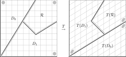
Figure 2.1. The piecewise affine map $T$ and the set $\mathcal{R}$, $\lambda=\gamma=\frac{1+\sqrt{5}}{2}$.

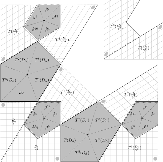
Figure 2.2. The trajectory of the scaled domains and the (gray) set $\mathcal{P}$, $\lambda=\gamma$. ($\tilde{\beta}^{k}$ stands for $T^{k}(D_{\tilde{\beta}})$.)

In Figure 2.2, we scale $D_{0}$ and $D_{1}$ by the factor $1/\gamma^{2}$ and follow their $T$-trajectory until the return to $\mathcal{D}/\gamma^{2}$. Let $\mathcal{P}$ be the set of points in $\mathcal{D}$ which are not eventually mapped to $\mathcal{D}/\gamma^{2}$, i.e.,

$$\mathcal{P}=D_{\alpha}\cup T(D_{\alpha})\cup D_{\beta}\cup T(D_{\beta})\cup T^{2}(D_{\beta}),$$

where $D_{\alpha}$ is the closed pentagon $\{(x,y)\in D_{0}:y\geq 1/\gamma^{2},x+y\leq 1,y\leq(1+x)/\gamma\}$ and $D_{\beta}$ is the open pentagon $\mathcal{R}/\gamma^{2}\setminus\{(0,0)\}$. (In Figure 2.2, $D_{\alpha}$ is split up into $\{T^{k}(D_{\tilde{\alpha}}):k\in\{0,2,4,6,8\}\}$, and $D_{\beta}$ is split up into $\{T^{k}(D_{\tilde{\beta}}):k\in\{0,3,6,9,12\}\}$.) All points in $\mathcal{P}$ are periodic (with minimal period lengths $2,3,10$ or $15$). Figures 2.1 and 2.2 show that the action of the first return map on $\mathcal{D}/\gamma^{2}$ is similar to the action of $T$ on $\mathcal{D}$, more precisely,

(2.2) $$\frac{T(z)}{\gamma^{2}}=\left\{\begin{array}[]{cl}T(z/\gamma^{2})&\mbox{if }z\in D_{0},\vspace{1mm}\\ T^{6}(z/\gamma^{2})&\mbox{if }z\in D_{1}.\end{array}\right.$$

For $z\in\mathcal{D}\setminus\mathcal{P}$, let $s(z)=\min\{m\geq 0:T^{m}(z)\in\mathcal{D}/\gamma^{2}\}$. (Figure 2.2 shows $s(z)\leq 5$.) By the map

$$S:\ \mathcal{D}\setminus\mathcal{P}\to\mathcal{D},\quad z\mapsto\gamma^{2}T^{s(z)}(z),$$

we can completely characterize the periodic points. For $z\in[0,1)^{2}$, denote by $\pi(z)$ the minimal period length if $(T^{k}(z))_{k\in\mathbb{Z}}$ is periodic and set $\pi(z)=\infty$ else.

Theorem 2.1.

$(T^{k}(z))_{k\in\mathbb{Z}}$ is periodic if and only if $z\in\mathcal{R}$ or $S^{n}(z)\in\mathcal{P}$ for some $n\geq 0$.

We postpone the proof to Section 3, where the more general Proposition 3.3 and Theorem 3.4 are proved (with $U(z)=z/\gamma^{2}$, $R(z)=z$, $\hat{T}(z)=T(z)$, $\hat{\pi}(z)=\pi(z)$, and $z\in D_{1}$ or $T(z)\in D_{1}$ for all $z\in\mathcal{D}$, $|\sigma^{n}(1)|\to\infty$, see below).

(2.2) and Figure 2.2 suggest to define a substitution (or morphism) $\sigma$ on the alphabet $\mathcal{A}=\{0,1\}$, i.e., a map $\sigma:\mathcal{A}\to\mathcal{A}^{*}$ (where $\mathcal{A}^{*}$ denotes the set of words with letters in $\mathcal{A}$), by

$$\sigma:\quad 0\mapsto 0\qquad 1\mapsto 101101$$

in order to code the trajectory of the scaled domains until their return to $\mathcal{D}/\gamma^{2}$: We have $T^{k-1}(D_{\ell}/\gamma^{2})\subseteq D_{\sigma(\ell)[k]}$ and $T^{|\sigma(\ell)|}(z/\gamma^{2})=T(z)/\gamma^{2}$ for all $z\in D_{\ell}$, where $w[k]$ denotes the $k$-th letter of the word $w$ and $|w|$ denotes its length. Furthermore, we have $T^{k}(D_{\ell}/\gamma^{2})\cap\mathcal{D}/\gamma^{2}=\emptyset$ for $1\leq k<|\sigma(\ell)|$. Extend the definition of $\sigma$ naturally to words in $\mathcal{A}^{*}$ by setting $\sigma(vw)=\sigma(v)\sigma(w)$, where $vw$ denotes the concatenation of $v$ and $w$. Then we get the following lemma, which resembles Proposition 1 by Poggiaspalla [24].

Lemma 2.2.

For every integer $n\geq 0$ and every $\ell\in\{0,1\}$, we have

• $T^{|\sigma^{n}(\ell)|}(z/\gamma^{2n})=T(z)/\gamma^{2n}$ for all $z\in D_{\ell}$,

• $T^{k-1}(D_{\ell}/\gamma^{2n})\subseteq D_{\sigma^{n}(\ell)[k]}$ for all $k$, $1\leq k\leq|\sigma^{n}(\ell)|$

• $T^{k}(D_{\ell}/\gamma^{2n})\cap\mathcal{D}/\gamma^{2n}=\emptyset$ for all $k$, $1\leq k<|\sigma^{n}(\ell)|$.

The proof is again postponed to Section 3, Lemma 3.1. This lemma allows to determine the minimal period lengths: If $z\in D_{\alpha}$, then

$$T^{|\sigma^{n}(0101010101)|}(z/\gamma^{2n})=T^{|\sigma^{n}(101010101)|}(T(z)/\gamma^{2n})=\cdots=T^{10}(z)/\gamma^{2n}=z/\gamma^{2n}$$

for all $n\geq 0$. The only points of the form $T^{k}(z/\gamma^{2n})$, $1\leq k\leq 5|\sigma^{n}(01)|$, which lie in $\mathcal{D}/\gamma^{2n}$ are the points $T^{m}(z)/\gamma^{2n}$, $1\leq m\leq 9$, which are all different from $z/\gamma^{2n}$ if $\pi(z)=10$. Therefore, we obtain $\pi(z/\gamma^{2n})=5|\sigma^{n}(01)|$ in this case. A point $\tilde{z}$ lies in the trajectory of $z/\gamma^{2n}$ if and only if $S^{n}(\tilde{z})=T^{m}(z)$ for some $m\in\mathbb{Z}$, see Lemma 3.2. This implies $\pi(\tilde{z})=5|\sigma^{n}(01)|$ for these $\tilde{z}$ as well. The period lengths of all points are given by the following theorem.

Theorem 2.3.

If $\lambda=\gamma$, then the minimal period lengths $\pi(z)$ of $(T^{k}(z))_{k\in\mathbb{Z}}$ are

$1$ if $z=(0,0)$ or $z=(\frac{\gamma^{2}}{\gamma^{2}+1},\frac{\gamma^{2}}{\gamma^{2}+1})$ $5$ if $z\in\mathcal{R}\setminus\{(0,0),(\frac{\gamma^{2}}{\gamma^{2}+1},\frac{\gamma^{2}}{\gamma^{2}+1})\}$ $(5\cdot 4^{n}+1)/3$ if $S^{n}(z)=T^{m}(\frac{1/\gamma}{\gamma^{2}+1},\frac{2}{\gamma^{2}+1})$ for some $n\geq 0$, $m\in\{0,1\}$ $5(5\cdot 4^{n}+1)/3$ if $S^{n}(z)\in T^{m}\big{(}D_{\alpha}\setminus\{(\frac{1/\gamma}{\gamma^{2}+1},\frac{2}{\gamma^{2}+1})\}\big{)}$ for some $n\geq 0$, $m\in\{0,1\}$ $(10\cdot 4^{n}-1)/3$ if $S^{n}(z)=T^{m}(\frac{1}{\gamma^{2}+1},\frac{1}{\gamma^{2}+1})$ for some $n\geq 0$, $m\in\{0,1,2\}$ $5(10\cdot 4^{n}-1)/3$ if $S^{n}(z)\in T^{m}\big{(}D_{\beta}\setminus\{(\frac{1}{\gamma^{2}+1},\frac{1}{\gamma^{2}+1})\}\big{)}$ for some $n\geq 0$, $m\in\{0,1,2\}$ $\infty$ if $S^{n}(z)\in\mathcal{D}\setminus\mathcal{P}$ for all $n\geq 0$.

The minimal period length of $(a_{k})_{k\in\mathbb{Z}}$ is $\pi(\{\gamma a_{k-1}\},\{\gamma a_{k}\})$ (which does not depend on $k$).

Proof.

By Theorem 2.1, Proposition 3.3 and the remarks preceding the theorem, it suffices to calculate $|\sigma^{n}(0)|$ and $|\sigma^{n}(1)|$. Clearly, we have $|\sigma^{n}(0)|=1$ for all $n\geq 0$ and thus

$$|\sigma^{n}(1)|=|\sigma^{n-1}(101101)|=4|\sigma^{n-1}(1)|+2=4(5\cdot 4^{n-1}-2)/3+2=(5\cdot 4^{n}-2)/3.$$

If $S^{n}(z)\in T^{m}(D_{\alpha})$, then $\pi(z)=|\sigma^{n}(01)|$ and $\pi(z)=5|\sigma^{n}(01)|$ respectively. If $S^{n}(z)\in T^{m}(D_{\beta})$, then $\pi(z)=|\sigma^{n}(101)|$ and $\pi(z)=5|\sigma^{n}(101)|$ respectively. ∎

Now consider aperiodic points $z\in[0,1)^{2}$, i.e., $S^{n}(z)\in\mathcal{D}\setminus\mathcal{P}$ for all $n\geq 0$. We can write

$$S(z)=\gamma^{2}T^{s(z)}(z)=\gamma^{2}\big{(}zA^{s(z)}+t(z)\big{)}$$

for some $t(z)$ by using (2.1). Note that $T(z)=zA$ for $z\in D_{0}$ and $T(z)=zA+(0,1)$ for $z\in D_{1}$. For $z\in\mathcal{D}/\gamma^{2}$, we have $s(z)=0$ and $t(z)=0$. For $z\in T^{k}(D_{1}/\gamma^{2})$, $1\leq k\leq 5$, we have $s(z)=6-k$,

$$t(z)=\left\{\begin{array}[]{ll}(0,1)&\mbox{if }s(z)\in\{1,2\},\\ (0,1)A^{2}+(0,1)=(1/\gamma,1/\gamma^{2})&\mbox{if }s(z)=3,\\ (0,1)A^{3}+(0,1)A^{2}+(0,1)=(0,-1/\gamma)&\mbox{if }s(z)\in\{4,5\}.\end{array}\right.$$

We obtain inductively

$$S^{n}(z)=\gamma^{2n}zA^{s(z)+s(S(z))+\ldots+s(S^{n-1}(z))}+\sum_{k=0}^{n-1}\gamma^{2(n-k)}t(S^{k}(z))A^{s(S^{k+1}(z))+\cdots+s(S^{n-1}(z))}.$$

If $z\in\mathbb{Q}(\gamma)^{2}$, then we have

$$(S^{n}(z))^{\prime}=\frac{\left(zA^{s(z)+s(S(z))+\cdots+s(S^{n-1}(z))}\right)^{\prime}}{\gamma^{2n}}+\sum_{k=0}^{n-1}\frac{\left(t(S^{k}(z))A^{s(S^{k+1}(z))+\cdots+s(S^{n-1}(z))}\right)^{\prime}}{\gamma^{2(n-k)}}\,$$

$$\left\|(S^{n}(z))^{\prime}\right\|_{\infty}\leq\frac{\max_{h\in\mathbb{Z}}\|(zA^{h})^{\prime}\|_{\infty}}{\gamma^{2n}}+\sum_{k=0}^{n-1}\frac{\max_{h\in\mathbb{Z},w\in\mathcal{D}\setminus\mathcal{P}}\|(t(w)A^{h})^{\prime}\|_{\infty}}{\gamma^{2{n-k}}}\,,$$

where $z^{\prime}=(x^{\prime},y^{\prime})$ if $z=(x,y)$ and $x^{\prime},y^{\prime}$ are the algebraic conjugates of $x,y$. Since

$$t(z)A^{h}\in\big{\{}(0,0),\ (0,1),(1,1/\gamma),(1/\gamma,-1/\gamma),(-1/\gamma,-1),(-1,0),\\ (1/\gamma,1/\gamma^{2}),(1/\gamma^{2},-1/\gamma^{2}),(-1/\gamma^{2},-1/\gamma),(-1/\gamma,0),(0,1/\gamma),\\ (0,-1/\gamma),(-1/\gamma,-1/\gamma^{2}),(-1/\gamma^{2},1/\gamma^{2}),(1/\gamma^{2},1/\gamma),(1/\gamma,0)\big{\}}$$

and $zA^{h}$ takes only the values $z$, $zA$, $zA^{2}$, $zA^{3}$ and $zA^{4}$, we obtain

$$\left\|(S^{n}(z))^{\prime}\right\|_{\infty}\leq\frac{\max_{h\in\mathbb{Z}}\|(zA^{h})^{\prime}\|_{\infty}}{\gamma^{2n}}+\sum_{k=0}^{n-1}\frac{\gamma^{2}}{\gamma^{2(n-k)}}<\frac{C(z)}{\gamma^{2n}}+\gamma$$

for some constant $C(z)$. If $z\in(\frac{1}{Q}\mathbb{Z}[\gamma])^{2}$ for some integer $Q\geq 1$, then $S^{n}(z)\in(\frac{1}{Q}\mathbb{Z}[\gamma])^{2}$. Since there exist only finitely many points $w\in(\frac{1}{Q}\mathbb{Z}[\gamma]\cap[0,1))^{2}$ with $\|w^{\prime}\|_{\infty}<C(z)+\gamma$, we must have $\|(S^{n}(z))^{\prime}\|_{\infty}\leq\gamma$ for some $n\geq 0$, which proves the following proposition.

Proposition 2.4.

Let $z\in(\frac{1}{Q}\mathbb{Z}[\gamma]\cap[0,1))^{2}$ be an aperiodic point. Then there exists an aperiodic point $\tilde{z}\in(\frac{1}{Q}\mathbb{Z}[\gamma])^{2}\cap\mathcal{D}$ with $\|\tilde{z}^{\prime}\|_{\infty}\leq\gamma$.

For every denominator $Q\geq 1$, it is therefore sufficient to check the periodicity of the (finite set of) points $z\in(\frac{1}{Q}\mathbb{Z}[\gamma])^{2}\cap\mathcal{D}$ with $\|z^{\prime}\|_{\infty}\leq\gamma$ in order to determine if all points in $(\frac{1}{Q}\mathbb{Z}[\gamma]\cap[0,1))^{2}$ are periodic.

For $Q=1$, we have to consider $z=(x,y)\in\mathcal{D}$ with $x,y\in\mathbb{Z}[\gamma]\cap[0,1)$ and $|x^{\prime}|,|y^{\prime}|\leq\gamma$, hence $(x,y)\in\{0,1/\gamma\}^{2}$. Since $(0,0)$ and $(1/\gamma,1/\gamma)$ are in $\mathcal{R}$, it only remains to check the periodicity of $(0,1/\gamma)$ and $(1/\gamma,0)$. These two points lie in $\mathcal{P}$, thus Conjecture 1.1 is proved for $\lambda=\gamma$.

For $Q=2$, a short inspection shows that all points $z\in(\frac{1}{2}\mathbb{Z}[\gamma]\cap[0,1))^{2}$ are periodic as well. The situation is completely different for $Q=3$, and we have

$$S(0,1/3) =(0,\gamma^{2}/3),\qquad S(0,\gamma^{2}/3)=\gamma^{2}\big{(}(0,\gamma^{2}/3)A^{5}+(0,-1/\gamma)\big{)}=(0,2/3),$$

$$S(0,2/3) =\gamma^{2}\big{(}(0,2/3)A^{5}+(0,-1/\gamma)\big{)}=\big{(}0,1/(3\gamma^{2})\big{)},\quad S^{4}(0,1/3)=S\big{(}0,1/(3\gamma^{2})\big{)}=(0,1/3).$$

This implies $S^{n}(0,1/3)\in\mathcal{D}\setminus\mathcal{P}$ for all $n\geq 0$ and $\pi(0,1/3)=\infty$ by Theorem 2.3.

Theorem 2.5.

$\pi(z)$ is finite for all points $z\in(\mathbb{Z}[\gamma]\cap[0,1))^{2}$, but $(T^{k}(0,1/3))_{k\in\mathbb{Z}}$ is aperiodic.

Figure 2.3. Aperiodic points, $\lambda=\gamma$.

Figure 2.4. Aperiodic points, $\lambda=-1/\gamma$.

3. General description of the method

In this section, we generalize the method presented in Section 2 in order to make it applicable for $\lambda=-\gamma,\pm 1/\gamma,\pm\sqrt{2},\pm\sqrt{3}$.

For the moment, we only need that $T:X\to X$ is a bijective map on a set $X$. Fix $\mathcal{D}\subseteq X$, let

$$\mathcal{R}=\{z\in X:\ T^{m}(z)\not\in\mathcal{D}\mbox{ for all }m\geq 0\}$$

set $r(z)=\min\{m\geq 0:T^{m}(z)\in\mathcal{D}\}$ for $z\in X\setminus\mathcal{R}$, and

$$R:\ X\setminus\mathcal{R}\to\mathcal{D},\qquad R(z)=T^{r(z)}(z).$$

Let $\hat{T}$ be the first return map (of the iterates by $T$) on $\mathcal{D}$, i.e.,

$$\hat{T}:\ \mathcal{D}\to\mathcal{D},\qquad\hat{T}(z)=RT(z)=T^{r(T(z))+1}(z),$$

in particular $\hat{T}(z)=T(z)$ if $T(z)\in\mathcal{D}$. Let $\mathcal{A}$ be a finite set, $\{D_{\ell}:\ell\in\mathcal{A}\}$ a partition of $\mathcal{D}$ and define a coding map $\iota:\mathcal{D}\to\mathcal{A}^{\mathbb{Z}}$ by $\iota(z)=(\iota_{k}(z))_{k\in\mathbb{Z}}$ such that $\hat{T}^{k}(z)\in D_{\iota_{k}(z)}$ for all $k\in\mathbb{Z}$. Let $U:\mathcal{D}\to\mathcal{D}$, $\varepsilon\in\{-1,1\}$ and $\sigma$ a substitution on $\mathcal{A}$ such that, for every $\ell\in\mathcal{A}$ and $z\in D_{\ell}$,

$$U\hat{T}(z)=\hat{T}^{\varepsilon|\sigma(\ell)|}U(z),$$

$\hat{T}^{\varepsilon k}U(z)\not\in U(\mathcal{D})$ for all $k$, $1\leq k<|\sigma(\ell)|$, and

$$\sigma(\ell)=\left\{\begin{array}[]{ll}\iota_{0}(U(z))\,\iota_{1}(U(z))\,\cdots\,\iota_{|\sigma(\ell)|-1}(U(z))&\mbox{if }\varepsilon=1,\\ \iota_{-|\sigma(\ell)|}(U(z))\,\cdots\,\iota_{-2}(U(z))\,\iota_{-1}(U(z))&\mbox{if }\varepsilon=-1.\end{array}\right.$$

Then the following lemma holds.

Lemma 3.1.

For every integer $n\geq 0$, every $\ell\in\mathcal{A}$ and $z\in D_{\ell}$, we have

$$U^{n}\hat{T}(z)=\hat{T}^{\varepsilon^{n}|\sigma^{n}(\ell)|}U^{n}(z),$$

$\hat{T}^{\varepsilon^{n}k}U^{n}(z)\not\in U^{n}(\mathcal{D})$ for all $k$, $1\leq k<|\sigma^{n}(\ell)|$, and

$$\begin{array}[]{cl}\iota_{0}(U^{n}(z))\,\iota_{1}(U^{n}(z))\,\cdots\,\iota_{|\sigma^{n}(\ell)|-1}(U^{n}(z))=\sigma^{n}(\ell)&\mbox{if }\varepsilon=1,\\ \iota_{0}(U^{n}(z))\,\iota_{1}(U^{n}(z))\,\cdots\,\iota_{|\sigma^{n}(\ell)|-1}(U^{n}(z))=(\sigma\bar{\sigma})^{n/2}(\ell)&\mbox{if }\varepsilon=-1,\varepsilon^{n}=1,\\ \iota_{-|\sigma^{n}(\ell)|}(U^{n}(z))\,\cdots\,\iota_{-2}(U^{n}(z))\,\iota_{-1}(U^{n}(z))=(\sigma\bar{\sigma})^{(n-1)/2}\sigma(\ell)&\mbox{if }\varepsilon=-1,\varepsilon^{n}=-1,\end{array}$$

where $\bar{\sigma}(\ell)=\ell_{m}\cdots\ell_{2}\ell_{1}$ if $\sigma(\ell)=\ell_{1}\ell_{2}\cdots\ell_{m}$.

Proof.

The lemma is trivially true for $n=0$, and for $n=1$ by the assumptions on $\sigma$. If we suppose inductively that it is true for $n-1$, then let $\sigma(\ell)=\ell_{1}\ell_{2}\cdots\ell_{m}$ if $\varepsilon=1$, $\sigma(\ell)=\ell_{m}\cdots\ell_{2}\ell_{1}$ if $\varepsilon=-1$, and we obtain (by another induction) for all $j$, $1\leq j\leq m$,

(3.1) $$\hat{T}^{\varepsilon^{n}|\sigma^{n-1}(\ell_{1}\cdots\ell_{j-1}\ell_{j})|}U^{n}(z)=\hat{T}^{\varepsilon^{n}|\sigma^{n-1}(\ell_{j})|}U^{n-1}\hat{T}^{\varepsilon(j-1)}U(z)=U^{n-1}\hat{T}^{\varepsilon j}U(z).$$

If $\varepsilon=1$, then this follows immediately from the induction hypothesis; if $\varepsilon=-1$, then this follows by setting $k=|\sigma^{n-1}(\ell_{j})|$ in

(3.2) $$\hat{T}^{(-1)^{n}k}U^{n-1}\hat{T}\big{(}\hat{T}^{-j}U(z)\big{)}=\hat{T}^{(-1)^{n}(k-|\sigma^{n-1}(\ell_{j})|)}U^{n-1}\hat{T}^{-j}U(z).$$

Therefore, we have

$$\hat{T}^{\varepsilon^{n}|\sigma^{n}(\ell)|}U^{n}(z)=\hat{T}^{\varepsilon^{n}|\sigma^{n-1}(\ell_{1}\cdots\ell_{m-1}\ell_{m})|}U^{n}(z)=U^{n-1}\hat{T}^{\varepsilon m}U(z)=U^{n-1}\hat{T}^{\varepsilon|\sigma(\ell)|}U(z)=U^{n}\hat{T}(z).$$

If $\varepsilon=1$, then (3.1) implies that

$$\iota_{0}(U^{n}(z))\cdots\iota_{|\sigma^{n}(\ell)|-1}(U^{n}(z))=\big{(}\iota_{0}(U^{n-1}U(z))\cdots\iota_{|\sigma^{n-1}(\ell_{1})|-1}(U^{n-1}U(z))\big{)}\cdots\\ \big{(}\iota_{0}(U^{n-1}\hat{T}^{m-1}U(z))\cdots\iota_{|\sigma^{n-1}(\ell_{m})|-1}(U^{n-1}\hat{T}^{m-1}U(z))\big{)}=\sigma^{n-1}(\ell_{1})\cdots\sigma^{n-1}(\ell_{m})=\sigma^{n}(\ell);$$

if $\varepsilon=-1$ and $\varepsilon^{n}=1$, then (3.1) and (3.2) provide

$$\iota_{0}(U^{n}(z))\cdots\iota_{|\sigma^{n}(\ell)|-1}(U^{n}(z)) =\big{(}\iota_{-|\sigma^{n-1}(\ell_{1})|}(U^{n-1}T^{-1}U(z))\cdots\iota_{-1}(U^{n-1}T^{-1}U(z))\big{)}$$

$$\quad\cdots\big{(}\iota_{-|\sigma^{n-1}(\ell_{m})|}(U^{n-1}\hat{T}^{-m}U(z))\cdots\iota_{-1}(U^{n-1}\hat{T}^{-m}U(z))\big{)}$$

$$=(\sigma\bar{\sigma})^{(n-2)/2}\sigma(\ell_{1})\cdots(\sigma\bar{\sigma})^{(n-2)/2}\sigma(\ell_{m})=(\sigma\bar{\sigma})^{n/2}(\ell);$$

if $\varepsilon=-1$ and $\varepsilon^{n}=-1$, then

$$\iota_{-|\sigma^{n}(\ell)|}(U^{n}(z))\cdots\iota_{-1}(U^{n}(z)) =\big{(}\iota_{0}(U^{n-1}T^{-m}U(z))\cdots\iota_{|\sigma^{n-1}(\ell_{m})|-1}(U^{n-1}T^{-m}U(z))\big{)}$$

$$\quad\cdots\big{(}\iota_{0}(U^{n-1}\hat{T}^{-1}U(z))\cdots\iota_{|\sigma^{n-1}(\ell_{1})|}(U^{n-1}\hat{T}^{-1}U(z))\big{)}$$

$$=(\sigma\bar{\sigma})^{(n-1)/2}(\ell_{m})\cdots(\sigma\bar{\sigma})^{(n-1)/2}(\ell_{1})=(\sigma\bar{\sigma})^{(n-1)/2}\sigma(\ell).$$

By (3.1), (3.2) and the induction hypothesis, the only points in $(\hat{T}^{\varepsilon^{n}k}U^{n}(z))_{1\leq k<|\sigma^{n}(\ell)|}$ lying in $U^{n-1}(\mathcal{D})$ are $U^{n}\hat{T}^{\varepsilon j}(z)$, $1\leq j<|\sigma(\ell)|$. Since $\hat{T}^{\varepsilon j}(z)\not\in U(\mathcal{D})$ for these $j$, the lemma is proved. ∎

Remark. If $\tilde{z}=\hat{T}^{-1}(z)\in D_{\ell}$, then $U^{n}\hat{T}(\tilde{z})=\hat{T}^{\varepsilon^{n}|\sigma^{n}(\ell)|}U^{n}(\tilde{z})$, thus $U^{n}\hat{T}^{-1}(z)=T^{-\varepsilon^{n}|\sigma^{n}(\ell)|}U^{n}(z)$.

As in Section 2, a key role will be played by the map $S$. Assume that $U$ is injective, let

$$\mathcal{P}=\{z\in\mathcal{D}:\ \hat{T}^{m}(z)\not\in U(\mathcal{D})\mbox{ for all }m\in\mathbb{Z}\},$$

fix $\hat{s}(z)=\min\{m\geq 0:\hat{T}^{m}(z)\in U(\mathcal{D})\}$ or $\hat{s}(z)=\max\{m\leq 0:\hat{T}^{m}(z)\in U(\mathcal{D})\}$ for every $z\in\mathcal{D}\setminus\mathcal{P}$, let $s(z)\in\mathbb{Z}$ be such that $\hat{T}^{\hat{s}(z)}(z)=T^{s(z)}(z)$, and define

$$S:\ \mathcal{D}\setminus\mathcal{P}\to\mathcal{D},\qquad z\mapsto U^{-1}\hat{T}^{\hat{s}(z)}(z)=U^{-1}T^{s(z)}(z).$$

Remark. Allowing $s(z)$ and $\hat{s}(z)$ to be negative decreases the $\delta$ in Proposition 3.5 in some cases.

Lemma 3.2.

If $S^{n}R(z)$ exists, then we have some $m\geq 0$ such that $U^{n}S^{n}R(z)=T^{m}(z)$, and

$$\tilde{z}=T^{m}(z)\mbox{ for some }m\in\mathbb{Z}\mbox{ if and only if }S^{n}R(\tilde{z})=\hat{T}^{k}S^{n}R(z)\mbox{ for some }k\in\mathbb{Z}.$$

Proof.

Suppose that $S^{n}R(z)$ exists. Then we have

$$U^{n}\!S^{n}\!R(z)=U^{n-1}\hat{T}^{\hat{s}(S^{n-1}R(z))}S^{n-1}R(z)=\hat{T}^{m_{1}}U^{n-1}S^{n-1}R(z)=\cdots=\hat{T}^{m_{1}+\cdots+m_{n}}R(z)=T^{m}(z)$$

for some $m_{1},\ldots,m_{n},m\geq 0$.

If $S^{n}R(\tilde{z})=\hat{T}^{k}S^{n}R(z)$ for some $k\in\mathbb{Z}$, then let $m_{1},m_{2}\geq 0$ be such that $U^{n}S^{n}R(z)=T^{m_{1}}(z)$, $U^{n}S^{n}R(\tilde{z})=T^{m_{2}}(\tilde{z})$, and we have

$$T^{m_{2}}(\tilde{z})=U^{n}S^{n}R(\tilde{z})=U^{n}\hat{T}^{k}S^{n}R(z)=\hat{T}^{k_{1}}U^{n}S^{n}R(z)=T^{k_{2}+m_{1}}(z)$$

for some $k_{1},k_{2}\in\mathbb{Z}$, hence $\tilde{z}=T^{m}(z)$ with $m=k_{2}+m_{1}-m_{2}$.

If $\tilde{z}=T^{m}(z)$ for some $m\in\mathbb{Z}$ and $n=0$, then we have $S^{n}R(\tilde{z})=\hat{T}^{k_{n}}S^{n}R(z)$ for some $k_{n}\in\mathbb{Z}$. If we suppose inductively that this is true for $n-1$, then

$$S^{n}R(\tilde{z})=S\hat{T}^{k_{n-1}}S^{n-1}R(z)=S\hat{T}^{k_{n-1}-\hat{s}(S^{n-1}R(z))}US^{n}R(z)=SU\hat{T}^{k_{n}}S^{n}R(z)=\hat{T}^{k_{n}}S^{n}R(z)$$

for some $k_{n-1},k_{n}\in\mathbb{Z}$, and the statement is proved. ∎

If $rT$ is constant on every $D_{\ell}$, $\ell\in\mathcal{A}$, then we can define $\tau:\mathcal{A}\to\mathbb{N}$ by $\tau(\ell)=r(T(z))+1$ for $z\in D_{\ell}$ (cf. the definition of $\hat{T}$) and extend $\tau$ naturally to words $w\in\mathcal{A}^{*}$ by $\tau(w)=\sum_{\ell\in\mathcal{A}}|w|_{\ell}\tau(\ell)$.

Let $\pi(z)$, $\hat{\pi}(z)$ be the minimal period lengths of $(T^{k}(z))_{k\in\mathbb{Z}}$ and $(\hat{T}^{k}(z))_{k\in\mathbb{Z}}$ respectively, with $\pi(z)=\infty$, $\hat{\pi}(z)=\infty$ if the sequences are aperiodic. Then the following proposition holds.

Proposition 3.3.

If $\hat{\pi}(S^{n}R(z))=p$ and $\ell_{1}\cdots\ell_{p}=\iota_{0}(S^{n}R(z))\cdots\iota_{p-1}(S^{n}R(z))$, then we have

$$\hat{\pi}(R(z))=|\sigma^{n}(\ell_{1}\ell_{2}\cdots\ell_{p})|\quad\mbox{and}\quad\pi(z)=\tau(\sigma^{n}(\ell_{1}\ell_{2}\cdots\ell_{p}))\ \mbox{(if $\tau$ is well defined)}.$$

Proof.

Since $U^{n}S^{n}R(z)=T^{m}(z)=\hat{T}^{\hat{m}}R(z)$ for some $m,\hat{m}\in\mathbb{Z}$, and

$$T^{\tau(\sigma^{n}(\ell_{1}\ell_{2}\cdots\ell_{p}))}U^{n}S^{n}R(z)=\hat{T}^{|\sigma^{n}(\ell_{1}\ell_{2}\cdots\ell_{p})|}U^{n}S^{n}R(z)=U^{n}\hat{T}^{p}S^{n}R(z)=U^{n}S^{n}R(z),$$

we have $\hat{\pi}(R(z))\leq|\sigma^{n}(\ell_{1}\cdots\ell_{p})|$ and $\pi(z)\leq\tau(\sigma^{n}(\ell_{1}\cdots\ell_{p}))$ (if $\tau$ exists). Since $p$ is minimal, we can show similarly to the proof of Lemma 3.1 that these period lengths are minimal. ∎

We obtain the following characterization of periodic points $z\not\in\mathcal{R}$. Note that all points in $\mathcal{P}\cup\mathcal{R}$ are periodic in our cases, hence the characterization is complete.

Theorem 3.4.

Let $R,S,T,\mathcal{D},\mathcal{P},\mathcal{R},\sigma$ be as in the preceding paragraphs of this section. Assume that $\hat{\pi}(z)$ is finite for all $z\in\mathcal{P}$, and that for every $z\in\mathcal{D}\setminus\mathcal{P}$ there exist $m\in\mathbb{Z}$, $\ell\in\mathcal{A}$, such that $\hat{T}^{m}(z)\in D_{\ell}$ and $|\sigma^{n}(\ell)|\to\infty$ for $n\to\infty$. Then we have for $z\not\in\mathcal{R}$:

$$(T^{k}(z))_{k\in\mathbb{Z}}\mbox{ is periodic if and only if }S^{n}R(z)\in\mathcal{P}\mbox{ for some }n\geq 0.$$

Proof.

If $S^{n}R(z)\in\mathcal{P}$, then we have $\hat{\pi}(R(z))=\hat{\pi}(S^{n}R(z))<\infty$, which implies $\pi(z)<\infty$.

Suppose now that $S^{n}R(z)\in\mathcal{D}\setminus\mathcal{P}$ for all $n\geq 0$. Then we have $m_{n}\in\mathbb{Z}$ and $\ell_{n}\in\mathcal{A}$ such that $\hat{T}^{m_{n}}S^{n}R(z)\in D_{\ell_{n}}$ and $|\sigma^{n}(\ell_{n})|\to\infty$ for $n\to\infty$ (because $\mathcal{A}$ is finite). We have $U^{n}\hat{T}^{m_{n}}S^{n}R(z)=\hat{T}^{\tilde{m}_{n}}U^{n}S^{n}R(z)\in U^{n}(D_{\ell_{n}})$ for some $\tilde{m}_{n}\in\mathbb{Z}$, hence $\hat{T}^{\tilde{m}_{n}+k}U^{n}S^{n}R(z)\not\in U^{n}(\mathcal{D})$ for all $k$, $1\leq k<|\sigma^{n}(\ell_{n})|$, which implies $\pi(z)\geq\hat{\pi}(R(z))=\hat{\pi}(U^{n}S^{n}R(z))\geq|\sigma^{n}(\ell_{n})|$ for all $n\geq 0$, thus $\pi(z)=\infty$. ∎

Assume now $\lambda\in\{\pm\sqrt{2},\frac{\pm 1\pm\sqrt{5}}{2},\pm\sqrt{3}\}$, let $\lambda^{\prime}$ be its algebraic conjugate, $T:[0,1)^{2}\to[0,1)^{2}$,

(3.3) $$T(x,y)=(x,y)A+(0,\lceil x+\lambda^{\prime}y\rceil)\ \mbox{ with }\ A=\begin{pmatrix}0&-1\\ 1&-\lambda^{\prime}\end{pmatrix},$$

$$U(z)=V^{-1}(\kappa V(z))$$

with $0<\kappa<1$, $\kappa\in\mathbb{Z}[\lambda]$, $|\kappa\kappa^{\prime}|=1$, and $V(z)=\pm\kappa^{n}(z-v)$ some $v\in\mathbb{Z}[\lambda]^{2}$, $n\in\mathbb{Z}$. Let

$$t(z)=V\big{(}T^{s(z)}(z)\big{)}-V(z)A^{s(z)}$$

for $z\in\mathcal{D}\setminus\mathcal{P}$. Since $U^{-1}(z)=V^{-1}(V(z)/\kappa)$, we have

$$S(z)=U^{-1}T^{s(z)}(z)=V^{-1}\left(\frac{V(z)A^{s(z)}+t(z)}{\kappa}\right).$$

Note that $A^{h}=A^{0}$ for some $h\in\{5,8,10,12\}$,

$$T^{-1}(x,y)=(x,y)A^{-1}+(\lceil\lambda^{\prime}x+y\rceil,0)\ \mbox{ with }\ A^{-1}=\begin{pmatrix}-\lambda^{\prime}&1\\ -1&0\end{pmatrix},$$

and $T^{-1}(x,y)=(\tilde{x},\tilde{y})$ with $(\tilde{y},\tilde{x})=T(y,x)$. Since $|\hat{s}(z)|<\max_{\ell\in\mathcal{A}}|\sigma(\ell)|$, there exists only a finite number of values for $t(z)$, and we obtain the following proposition.

Proposition 3.5.

Let $T,V,\kappa$ be as above and the assumptions of Theorem 3.4 be satisfied. Suppose that $\pi(z)=\infty$ for some $z\in(\frac{1}{Q}\mathbb{Z}[\lambda]\cap[0,1))^{2}\setminus\mathcal{R}$, where $Q$ is a positive integer. Then there exists an aperiodic point $\tilde{z}\in(\frac{1}{Q}\mathbb{Z}[\lambda])^{2}\cap\mathcal{D}$ with

$$\|V(\tilde{z})^{\prime}\|_{\infty}\leq\delta,\quad\mbox{where }\delta=\frac{\max\{\|(t(z)A^{h})^{\prime}\|_{\infty}:\,z\in\mathcal{D}\setminus\mathcal{P},\,\pi(z)=\infty,\,h\in\mathbb{Z}\}}{|\kappa^{\prime}|-1}\,.$$

Proof.

First note that $\delta$ exists since $t(z)$ and $A^{h}$ take only finitely many values. If $\pi(z)=\infty$ for some $z\in(\frac{1}{Q}\mathbb{Z}[\lambda]\cap[0,1))^{2}\setminus\mathcal{R}$, then $S^{n}R(z)\in\mathcal{D}\setminus\mathcal{P}$ for all $n\geq 0$ by Theorem 3.4. In particular, $S^{n}R(z)$ is aperiodic as well. We use the abbreviations $s_{n}=s(S^{n}R(z))$ and $t_{n}=t(S^{n}R(z))$. Then we obtain inductively, for $n\geq 1$,

$$VS^{n}R(z)=\frac{VS^{n-1}R(z)A^{s_{n-1}}+t_{n-1}}{\kappa}=\frac{VR(z)A^{s_{0}+s_{1}+\cdots+s_{n-1}}}{\kappa^{n}}+\sum_{k=0}^{n-1}\frac{t_{k}A^{s_{k+1}+\cdots+s_{n-1}}}{\kappa^{n-k}}.$$

If we look at the algebraic conjugates, then note that $|\kappa^{\prime}|>1$, and we obtain

$$\left\|(VS^{n}R(z))^{\prime}\right\|_{\infty}<\frac{\left\|\big{(}VR(z)A^{s_{0}+s_{1}+\cdots+s_{n-1}}\big{)}^{\prime}\right\|_{\infty}}{|\kappa^{\prime}|^{n}}+\delta,$$

thus $\left\|(VS^{n}R(z))^{\prime}\right\|_{\infty}\leq\delta$ for some $n\geq 0$ (as in Section 2), and we can choose $\tilde{z}=S^{n}R(z)$. ∎

Remarks.

• The last proof shows that, for every $z\in(\mathbb{Q}(\lambda)\cap[0,1))^{2}\setminus\mathcal{R}$ with $\pi(z)=\infty$, there are only finitely many possibilities for $VS^{n}R(z)$, hence $(S^{n}R(z))_{n\geq 0}$ is eventually periodic.

• For every $z\in\mathcal{D}$ with $\pi(z)=\infty$, we have

  $$\qquad\quad V(z)=\Big{(}VS^{n}(z)\kappa^{n}-\sum_{k=0}^{n-1}t_{k}A^{s_{k+1}+\cdots+s_{n-1}}\kappa^{k}\Big{)}A^{-s_{0}-\cdots-s_{n-1}}=-\sum_{k=0}^{\infty}t_{k}A^{-\sum_{j=0}^{k}s(S^{j}(z))}\kappa^{k},$$

  which is a $\kappa$-expansion ($\kappa<1$) of $V(z)$ with (two-dimensional) “digits” $-t_{k}A^{-s_{0}-s_{1}-\cdots-s_{k}}$.

• As a consequence of Lemma 3.2 and the definition of $U$, for every aperiodic point $z\in[0,1)^{2}\setminus\mathcal{R}$ and every $c>0$, there exists some $m\in\mathbb{Z}$ such that $\|T^{m}(z)-v\|_{\infty}<c$.

• In all our cases, we have $\varepsilon=\kappa\kappa^{\prime}$.

4. The case $\lambda=-1/\gamma=\frac{1-\sqrt{5}}{2}=-2\cos\frac{2\pi}{5}$

Now we apply the method of Section 3 for $\lambda=-1/\gamma$, i.e., $\lambda^{\prime}=\gamma$. To this end, set

$$\mathcal{D}=\{(x,y)\in[0,1)^{2}:\,x+y\geq 3-\gamma\}=D_{0}\cup D_{1}$$

with $D_{0}=\{(x,y)\in\mathcal{D}:x+\gamma y>2\}$, $D_{1}=\{(x,y)\in\mathcal{D}:x+\gamma y\leq 2\}$. Figure 4.1 shows that $\hat{T}$ is given by $\hat{T}(z)=T^{\tau(\ell)}(z)$ if $z\in D_{\ell}$, $\ell\in\mathcal{A}=\{0,1\}$, with $\tau(0)=1$ and $\tau(1)=4$. The set which is left out by the iterates of $D_{0}$ and $D_{1}$ is $\mathcal{R}=\{(0,0)\}\cup D_{A}\cup D_{B}$, with

$$D_{A}=\{z\in[0,1)^{2}:T^{k+1}(z)=T^{k}(z)A+(0,1)\mbox{ for all }k\geq 0\},$$

$$D_{B}=\{z\in[0,1)^{2}:T^{k+1}(z)=T^{k}(z)A+(0,2)\mbox{ for all }k\geq 0\}.$$

As in Section 2, we have $T^{5}(z)=z$ for all $z\in\mathcal{R}$. If we set

$$U(z)=\frac{z}{\gamma^{2}}+\Big{(}\frac{1}{\gamma},\frac{1}{\gamma}\Big{)}=(1,1)-\frac{(1,1)-z}{\gamma^{2}},$$

$V(z)=(1,1)-z$, $\kappa=1/\gamma^{2}$, $\varepsilon=1$, and

$$\sigma:\ 0\mapsto 010\qquad 1\mapsto 01110$$

then Figure 4.2 shows that $\sigma$ satisfies the conditions in Section 3, and $\mathcal{P}=D_{\alpha}\cup D_{\beta}$ with $D_{\alpha}=U(D_{A})$, $D_{\beta}=U(D_{B})$. All points in $\mathcal{P}$ are periodic and $|\sigma^{n}(\ell)|\to\infty$ as $n\to\infty$ for all $\ell\in\mathcal{A}$. Therefore, all conditions of Proposition 3.3 and Theorem 3.4 are satisfied, and we obtain the following theorem.

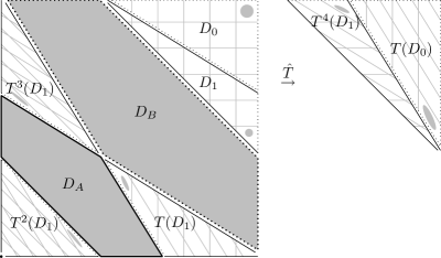
Figure 4.1. The map $\hat{T}$, $\hat{T}(D_{0})=T(D_{0})$, $\hat{T}(D_{1})=T^{4}(D_{1})$, and the (gray) set $\mathcal{R}$, $\lambda=-1/\gamma$.

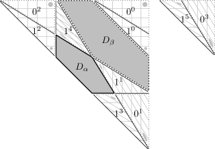
Figure 4.2. The trajectory of the scaled domains and $\mathcal{P}$, $\lambda=-1/\gamma$. ($\ell^{k}$ stands for $\hat{T}^{k}U(D_{\ell})$.)

Theorem 4.1.

If $\lambda=-1/\gamma$, then the period lengths $\pi(z)$ are

$1$ if $z\in\{(0,0),(\frac{1}{\gamma^{2}+1},\frac{1}{\gamma^{2}+1}),(\frac{2}{\gamma^{2}+1},\frac{2}{\gamma^{2}+1})\}$ $5$ for the other points of the pentagons $D_{A}$ and $D_{B}$ $2(5\cdot 4^{n}+1)/3$ if $S^{n}R(z)=(\frac{\gamma^{2}}{\gamma^{2}+1},\frac{\gamma^{2}}{\gamma^{2}+1})$ for some $n\geq 0$ $10(5\cdot 4^{n}+1)/3$ for the other points with $S^{n}R(z)\in D_{\alpha}$ for some $n\geq 0$ $(5\cdot 4^{n}-2)/3$ if $S^{n}R(z)=(\frac{3}{\gamma^{2}+1},\frac{3}{\gamma^{2}+1})$ for some $n\geq 0$ $5(5\cdot 4^{n}-2)/3$ for the other points with $S^{n}R(z)\in D_{\beta}$ for some $n\geq 0$ $\infty$ if $S^{n}R(z)\in\mathcal{D}\setminus\mathcal{P}$ for all $n\geq 0$.

Proof.

We easily calculate

$$\begin{pmatrix}|\sigma^{n}(0)|_{0}\\ |\sigma^{n}(0)|_{1}\end{pmatrix}=4^{n}\begin{pmatrix}1/3\\ 1/3\end{pmatrix}+\begin{pmatrix}2/3\\ -1/3\end{pmatrix},\qquad\begin{pmatrix}|\sigma^{n}(1)|_{0}\\ |\sigma^{n}(1)|_{1}\end{pmatrix}=4^{n}\begin{pmatrix}2/3\\ 2/3\end{pmatrix}+\begin{pmatrix}-2/3\\ 1/3\end{pmatrix},$$

hence $\tau(\sigma^{n}(0))=\frac{5}{3}4^{n}-\frac{2}{3}$, $\tau(\sigma^{n}(1))=\frac{10}{3}4^{n}+\frac{2}{3}$. If $S^{n}R(z)\in D_{\alpha}$, then $\pi(z)=\tau(\sigma^{n}(1))$ and $\pi(z)=\tau(\sigma^{n}(11111))$ respectively; if $S^{n}R(z)\in D_{\beta}$, then $\pi(z)=\tau(\sigma^{n}(0))$ and $\pi(z)=5\tau(\sigma^{n}(0))$ respectively. ∎

For $z\in U(\mathcal{D})$, we have $\hat{s}(z)=s(z)=0$ and $t(z)=(0,0)$. For the other $z\in\mathcal{D}\setminus\mathcal{P}$, we choose $\hat{s}(z)$ as follows and obtain the following $s(z),t(z)$:

$$z\in\hat{T}^{2}U(D_{0})\cup\hat{T}^{2}U(D_{1}):\ \hat{s}(z)=-2,\,s(z)=-5,\ t(z)=V(\hat{T}^{-2}(z))-V(z)=(-1/\gamma^{2},0)$$

$$z\in\hat{T}U(D_{1}):\ \hat{s}(z)=-1,\,s(z)=-1,\ t(z)=V(\hat{T}^{-1}(z))-V(z)A^{-1}=(1/\gamma,0)$$

$$z\in\hat{T}^{4}U(D_{1}):\ \hat{s}(z)=1,\,s(z)=1,\ t(z)=V(\hat{T}(z))-V(z)A=(0,1/\gamma)$$

$$z\in\hat{T}U(D_{0})\cup\hat{T}^{3}U(D_{1}):\ \hat{s}(z)=2,\,s(z)=5,\ t(z)=V(\hat{T}^{2}(z))-V(z)=(0,-1/\gamma^{2})$$

Observe the symmetry between positive and negative $\hat{s}(z)$ which is due to the symmetry of $T(x,y)$ and $T^{-1}(y,x)$ and the symmetry of $\mathcal{D}$. With

$$\{(1/\gamma,0)A^{h}:\,h\in\mathbb{Z}\}=\{(1/\gamma,0),\,(0,-1/\gamma),\,(-1/\gamma,1),\,(1,-1),\,(-1,1/\gamma)\},$$

we obtain $\delta\leq\max\{\|(t(z)A^{h})^{\prime}\|_{\infty}:\,z\in\mathcal{D}\setminus\mathcal{P},\,h\in\mathbb{Z}\}/\gamma=(1/\gamma^{2})^{\prime}/\gamma=\gamma$, as in Section 2. The following theorem shows that aperiodic points with $t(z)=(-1/\gamma^{2},0)$ exist, hence $\delta=\gamma$.

Theorem 4.2.

$\pi(z)$ is finite for all $z\in(\mathbb{Z}[\gamma]\cap[0,1))^{2}$, but $\pi\big{(}1-1/(3\gamma),1-2/(3\gamma)\big{)}=\infty$.

Proof.

By Proposition 3.5, we have to show that all $z\in\mathbb{Z}[\gamma]^{2}\cap\mathcal{D}$ with $\|V(z)^{\prime}\|_{\infty}\leq\gamma$ are periodic. Since $V(\mathcal{D})=\{(x,y):x>0,y>0,x+y\leq 1/\gamma\}$, we have to consider $x,y\in\mathbb{Z}[\gamma]\cap(0,1/\gamma)$ with $|x^{\prime}|,|y^{\prime}|\leq\gamma$. No such $x,y$ exist, hence the conjecture is proved for $\lambda=-1/\gamma$. Note that $\pi(z)$ is finite for all $z\in(\frac{1}{2}\mathbb{Z}[\gamma]\cap[0,1))^{2}$ as well. If $V(z)=\big{(}1/(3\gamma),2/(3\gamma)\big{)}$, then we have

$$VS(z) =\gamma^{2}\big{(}V(z)A^{5}+(0,-1/\gamma^{2})\big{)}=\big{(}\gamma/3,1/(3\gamma^{3})\big{)}$$

$$VS^{2}(z) =\gamma^{2}\big{(}VS(z)A^{-5}+(-1/\gamma^{2},0)\big{)}=\big{(}2/(3\gamma),1/(3\gamma)\big{)}$$

$$VS^{3}(z) =\gamma^{2}\big{(}VS^{2}(z)A^{-5}+(0,-1/\gamma^{2})\big{)}=\big{(}1/(3\gamma^{3}),\gamma/3)\big{)}$$

$$VS^{4}(z) =\gamma^{2}\big{(}VS^{3}(z)A^{5}+(0,-1/\gamma^{2})\big{)}=\big{(}1/(3\gamma),2/(3\gamma)\big{)}=V(z),$$

hence $S^{n}(z)\in\mathcal{D}\setminus\mathcal{P}$ for all $n\geq 0$ and $\pi(z)=\infty$ by Theorem 4.1. ∎

5. The case $\lambda=\sqrt{2}=-2\cos\frac{3\pi}{4}$

Let $\lambda=\sqrt{2}$ ($\lambda^{\prime}=-\sqrt{2}$) and set

$$\mathcal{D}=\{(x,y)\in[0,1)^{2}:\sqrt{2}-2<x-\sqrt{2}y<0,\ 0<\sqrt{2}x-y<\sqrt{2}-2\}=\bigcup\nolimits_{\ell\in\mathcal{A}=\{0,1,2,3\}}D_{\ell},$$

$$D_{0}=\{(x,y)\in\mathcal{D}:x<\sqrt{2}-1\},\quad D_{1}=\{(x,y)\in\mathcal{D}:x>\sqrt{2}-1,y\leq\sqrt{2}-1\},$$

$$D_{2}=\{(x,y)\in\mathcal{D}:x>\sqrt{2}-1,y>\sqrt{2}-1\},\quad D_{3}=\{(x,y)\in\mathcal{D}:x=\sqrt{2}-1\}.$$

Figure 5.1 shows that $\hat{T}(z)=T^{\tau(\ell)}(z)$ if $z\in D_{\ell}$, with $\tau(0)=5$, $\tau(1)=9$, $\tau(2)=3$, $\tau(3)=11$, and $\mathcal{R}=\{(0,0)\}\cup\bigcup_{k=0}^{3}T^{k}(D_{A})\cup\bigcup_{k=0}^{5}T^{k}(D_{B})$ with $D_{A}=\{(0,y):1-1/\sqrt{2}<y<1/\sqrt{2}\}$, $D_{B}=\{(0,1/\sqrt{2})\}$. If we set $U(z)=(\sqrt{2}-1)z$, $V(z)=z$, $\kappa=\sqrt{2}-1$, $\varepsilon=-1$, and

$$\sigma:\ 0\mapsto 010\qquad 1\mapsto 000\qquad 2\mapsto 0\qquad 3\mapsto 030,$$

then Figure 5.2 shows that $\sigma$ satisfies the conditions in Section 3, and

$$\mathcal{P}=\{(x,y)\in\mathcal{D}:x,y\geq\sqrt{2}-1\}=D_{\alpha}\cup D_{\beta}\cup\hat{T}(D_{\beta})\cup D_{\zeta}$$

with $D_{\alpha}=D_{2}$, $D_{\beta}=\{(x,\sqrt{2}-1):\sqrt{2}-1<x<2-\sqrt{2}\}$ and $D_{\zeta}=\{(\sqrt{2}-1,\sqrt{2}-1)\}$. All points in $\mathcal{P}$ are periodic and $|\sigma^{n}(\ell)|\to\infty$ as $n\to\infty$ for all $\ell\in\mathcal{A}$. Therefore, all conditions of Proposition 3.3 and Theorem 3.4 are satisfied, and we obtain the following theorem.

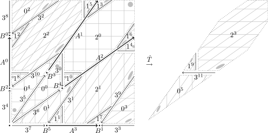
Figure 5.1. The map $\hat{T}$ and the set $\mathcal{R}$, $\lambda=\sqrt{2}$. ($\ell^{k}$ stands for $T^{k}(D_{\ell})$.)

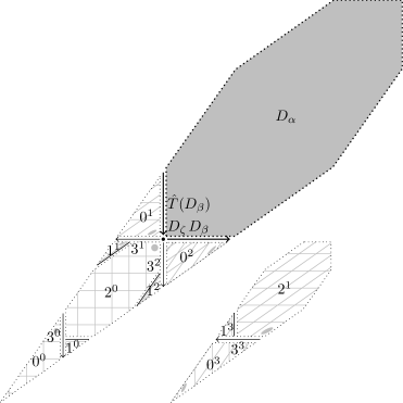
Figure 5.2. The trajectory of the scaled domains and $\mathcal{P}$, $\lambda=\sqrt{2}$. ($\ell^{k}$ stands for $\hat{T}^{-k}U(D_{\ell})$.)

Theorem 5.1.

If $\lambda=\sqrt{2}$, then the minimal period length $\pi(z)$ is

$1$ if $z=(0,0)$ $4$ if $z=T^{m}(0,1/2)$, $0\leq m\leq 3$ $8$ for the other points of $T^{m}(D_{A})$, $0\leq m\leq 3$ $6$ if $z=T^{m}(0,1/\sqrt{2})$, $0\leq m\leq 5$ $2\cdot 3^{n}+(-1)^{n}$ if $S^{n}R(z)=(1/\sqrt{2},1/\sqrt{2})$, $n\geq 0$ $8(2\cdot 3^{n}+(-1)^{n})$ for the other points with $S^{n}R(z)\in D_{\alpha}$ $4(3^{n+1}+1+(-1)^{n})$ if $S^{n}R(z)\in\{(1/2,\sqrt{2}-1),(\sqrt{2}-1,1/2)\}$, $n\geq 0$ $8(3^{n+1}+1+(-1)^{n})$ for the other points with $S^{n}R(z)\in D_{\beta}\cup\hat{T}(D_{\beta})$ $2\cdot 3^{n+1}+4+(-1)^{n}$ if $S^{n}R(z)=(\sqrt{2}-1,\sqrt{2}-1)$, $n\geq 0$ $\infty$ if $S^{n}R(z)\in\mathcal{D}\setminus\mathcal{P}$ for all $n\geq 0$.

Proof.

We easily calculate

$$\begin{pmatrix}|\sigma^{n}(0)|_{0}\\ |\sigma^{n}(0)|_{1}\end{pmatrix}=3^{n}\begin{pmatrix}3/4\\ 1/4\end{pmatrix}+(-1)^{n}\begin{pmatrix}1/4\\ -1/4\end{pmatrix},\qquad\begin{pmatrix}|\sigma^{n}(1)|_{0}\\ |\sigma^{n}(1)|_{1}\end{pmatrix}=3^{n}\begin{pmatrix}3/4\\ 1/4\end{pmatrix}+(-1)^{n}\begin{pmatrix}-3/4\\ 3/4\end{pmatrix}$$

and obtain $\tau(\sigma^{n}(0))=2\cdot 3^{n+1}-(-1)^{n}$, $\tau(\sigma^{n}(3))=\tau(\sigma^{n-1}(030))=2\cdot 3^{n+1}+4+(-1)^{n}$. If $S^{n}R(z)\in D_{\alpha}$ and $n\geq 1$, then $\pi(z)=\tau(\sigma^{n}(2))=\tau(\sigma^{n-1}(0))$ and $\pi(z)=8\tau(\sigma^{n-1}(0))$ respectively; if $S^{n}R(z)\in D_{\beta}$, then $\pi(z)=\tau(\sigma^{n}(13))=\tau(\sigma^{n-1}(000030))$ and $\pi(z)=2\tau(\sigma^{n-1}(000030))$ respectively; if $S^{n}R(z)=(\sqrt{2}-1,\sqrt{2}-1)$, then $\pi(z)=\tau(\sigma^{n}(3))$. The given $\pi(z)$ hold for $n=0$ as well. ∎

For $z\in\mathcal{D}\setminus(U(\mathcal{D})\cup\mathcal{P})$, we choose $\hat{s}(z)$ as follows and obtain the following $s(z),t(z)$:

$$z\in\hat{T}^{-2}U(D_{0}\cup D_{1}\cup D_{3}):\ \hat{s}(z)=-1,\,s(z)=-5,\ t(z)=\hat{T}^{-1}(z)-zA^{-5}=(\sqrt{2}-1,2-\sqrt{2})$$

$$z\in\hat{T}^{-1}U(D_{0}\cup D_{1}\cup D_{3}):\ \hat{s}(z)=1,\,s(z)=5,\ t(z)=\hat{T}(z)-zA^{5}=(2-\sqrt{2},\sqrt{2}-1)$$

This gives $\delta=(2+\sqrt{2})/\sqrt{2}=\sqrt{2}+1$ since

$$\{t(z)A^{h}:z\in\mathcal{D}\setminus\mathcal{P},h\in\mathbb{Z}\}=\pm\{(0,0),\ (2-\sqrt{2},\sqrt{2}-1),(\sqrt{2}-1,0),(0,1-\sqrt{2}),(1-\sqrt{2},\sqrt{2}-2)\}.$$

Theorem 5.2.

$\pi(z)$ is finite for all $z\in(\mathbb{Z}[\sqrt{2}]\cap[0,1))^{2}$, but $(T^{k}(\frac{3-\sqrt{2}}{4},\frac{2\sqrt{2}-1}{4}))_{k\in\mathbb{Z}}$ is aperiodic.

Proof.

We have to consider $z\in\mathbb{Z}[\sqrt{2}]^{2}\cap\mathcal{D}$ with $\|z^{\prime}\|_{\infty}\leq\delta=\sqrt{2}+1$. The only such point is $(\sqrt{2}-1,\sqrt{2}-1)=D_{\zeta}$, hence Conjecture 1.1 holds for $\lambda=\sqrt{2}$. It can be shown that all points in $(\frac{1}{2}\mathbb{Z}[\sqrt{2}]\cap[0,1))^{2}$ and $(\frac{1}{3}\mathbb{Z}[\sqrt{2}]\cap[0,1))^{2}$ are periodic as well. For $z=(\frac{3-\sqrt{2}}{4},\frac{2\sqrt{2}-1}{4})$, we have

$$S(z)=\big{(}zA^{5}+(2-\sqrt{2},\sqrt{2}-1)\big{)}/\kappa=(\sqrt{2}+1)\Big{(}\frac{9-6\sqrt{2}}{4},\sqrt{2}-\frac{5}{4}\Big{)}=\Big{(}\frac{3\sqrt{2}-3}{4},\frac{3-\sqrt{2}}{4}\Big{)},$$

$$S^{2}(z)=\big{(}S(z)A^{5}+(2-\sqrt{2},\sqrt{2}-1)\big{)}/\kappa=(\sqrt{2}+1)\Big{(}\frac{5-3\sqrt{2}}{4},\sqrt{2}-\frac{5}{4}\Big{)}=\Big{(}\frac{2\sqrt{2}-1}{4},\frac{3-\sqrt{2}}{4}\Big{)},$$

$S^{3}(z)=\big{(}S^{2}(z)A^{-5}+(\sqrt{2}-1,2-\sqrt{2})\big{)}/\kappa=(\frac{3-\sqrt{2}}{4},\frac{3\sqrt{2}-3}{4})$ and $S^{4}(z)=(\frac{3-\sqrt{2}}{4},\frac{2\sqrt{2}-1}{4})=z$. ∎

Figure 5.3. Aperiodic points, $\lambda=\sqrt{2}$.

Figure 5.4. Aperiodic points, $\lambda=-\sqrt{2}$.

6. The case $\lambda=-\sqrt{2}=-2\cos\frac{\pi}{4}$

Let $\lambda=-\sqrt{2}$ ($\lambda^{\prime}=\sqrt{2}$) and set

$$\mathcal{D}=\{(x,y)\in[0,1)^{2}:\sqrt{2}x+y>2\mbox{ or }x+\sqrt{2}y>2\}=\bigcup\nolimits_{\ell\in\mathcal{A}=\{0,1,2\}}D_{\ell},$$

with $D_{0}=\{(x,y)\in\mathcal{D}:x+\sqrt{2}y>2\}$ and $D_{1}=\{(x,y)\in\mathcal{D}:x+\sqrt{2}y<2\}$. Figure 6.1 shows that $\hat{T}(z)=T^{\tau(\ell)}(z)$ if $z\in D_{\ell}$, with $\tau(0)=1$, $\tau(1)=21$, $\tau(2)=31$, and

$$\mathcal{R}=\{(0,0)\}\cup D_{A}\cup D_{B}\cup\bigcup\nolimits_{k=0}^{3}T^{k}(D_{\Gamma})\cup\bigcup\nolimits_{k=0}^{9}T^{k}(D_{\Delta}),$$

$$D_{A}=\{(x,y):0\leq x,y\leq 3-2\sqrt{2}\}\setminus\{(0,0),(3-2\sqrt{2},3-2\sqrt{2})\},$$

$$D_{B}=\{z\in[0,1)^{2}:T^{k+1}(z)=T^{k}(z)A+(0,1)\mbox{ for all }k\in\mathbb{Z}\},$$

$$D_{\Gamma}=\{z\in[0,1)^{2}:T^{k+1}(z)=T^{k}(z)A+(0,2)\mbox{ for all }k\in\mathbb{Z}\},$$

$D_{\Delta}=\{(1/\sqrt{2},0)\}$. Set $\kappa=\sqrt{2}-1$, $V(z)=((1,1)-z)/\kappa=(\sqrt{2}+1)((1,1)-z)$, i.e.,

$$U(z)=(1,1)-(\sqrt{2}-1)\big{(}(1,1)-z\big{)}=(\sqrt{2}-1)z+(2-\sqrt{2},2-\sqrt{2}).$$

Then Figure 6.2 shows that the conditions in Section 3 are satisfied by

$$\sigma:\ 0\mapsto 010\qquad 1\mapsto 000\qquad 2\mapsto 020$$

with $\varepsilon=-1$ and $\mathcal{P}=D_{\alpha}\cup\bigcup_{k=0}^{5}\hat{T}^{k}(D_{\beta})\cup\bigcup_{k=0}^{2}\hat{T}^{k}(D_{\zeta})$ with

$$D_{\alpha}=\{z\in[0,1)^{2}:T^{k+1}(z)=T^{k}(z)A+(0,3)\mbox{ for all }k\in\mathbb{Z}\},$$

$D_{\beta}=\{(x,2-\sqrt{2}x):5-3\sqrt{2}<x<2\sqrt{2}-2\}$ and $D_{\zeta}=\{(8-5\sqrt{2},8-5\sqrt{2})\}$. All points in $\mathcal{P}$ are periodic and $|\sigma^{n}(\ell)|\to\infty$ as $n\to\infty$ for all $\ell\in\mathcal{A}$. Therefore, all conditions of Proposition 3.3 and Theorem 3.4 are satisfied, and we obtain the following theorem.

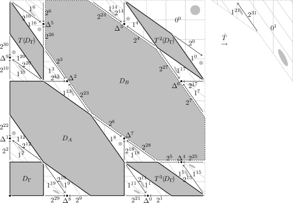
Figure 6.1. The map $\hat{T}$ and the set $\mathcal{R}$, $\lambda=-\sqrt{2}$. ($\ell^{k}$ stands for $T^{k}(D_{\ell})$.)

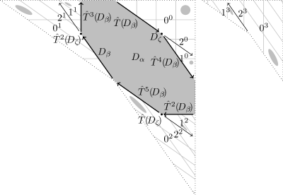
Figure 6.2. The trajectory of the scaled domains and $\mathcal{P}$, $\lambda=-\sqrt{2}$. ($\ell^{k}$ stands for $\hat{T}^{-k}U(D_{\ell})$.)

Theorem 6.1.

If $\lambda=-\sqrt{2}$, then the minimal period length $\pi(z)$ is

$1$ if $z\in\{(0,0),(1/\sqrt{2},1/\sqrt{2}),(2-\sqrt{2},2-\sqrt{2})\}$ $4$ if $z=T^{m}(3/2-\sqrt{2},3/2-\sqrt{2})$ for some $m\in\{0,1,2,3\}$ $10$ if $z=T^{m}(1/\sqrt{2},0)$ for some $m\in\{0,1,\ldots,9\}$ $8$ for the other points in $\mathcal{R}$ $2\cdot 3^{n+1}-5(-1)^{n}$ if $S^{n}R(z)=(3-3/\sqrt{2},3-3/\sqrt{2})$ for some $n\geq 0$ $8(2\cdot 3^{n+1}-5(-1)^{n})$ for the other points with $S^{n}R(z)\in D_{\alpha}$ $4(3^{n+2}+5-5(-1)^{n})$ if $S^{n}R(z)=\hat{T}^{m}\big{(}(9-5\sqrt{2})/2,5-3\sqrt{2}\big{)}$ for some $m\in\{0,\ldots,5\}$, $n\geq 0$ $8(3^{n+2}+5-5(-1)^{n})$ for the other points with $S^{n}R(z)\in\hat{T}^{m}(D_{\beta})$ $2\cdot 3^{n+2}+20-5(-1)^{n}$ if $S^{n}R(z)=\hat{T}^{m}(8-5\sqrt{2},8-5\sqrt{2})$ for some $m\in\{0,1,2\}$, $n\geq 0$ $\infty$ if $S^{n}R(z)\in\mathcal{D}\setminus\mathcal{P}$ for all $n\geq 0$.

Proof.

As for $\lambda=\sqrt{2}$, we have

$$\begin{pmatrix}|\sigma^{n}(0)|_{0}\\ |\sigma^{n}(0)|_{1}\end{pmatrix}=3^{n}\begin{pmatrix}3/4\\ 1/4\end{pmatrix}+(-1)^{n}\begin{pmatrix}1/4\\ -1/4\end{pmatrix},\qquad\begin{pmatrix}|\sigma^{n}(1)|_{0}\\ |\sigma^{n}(1)|_{1}\end{pmatrix}=3^{n}\begin{pmatrix}3/4\\ 1/4\end{pmatrix}+(-1)^{n}\begin{pmatrix}-3/4\\ 3/4\end{pmatrix},$$

hence $\tau(\sigma^{n}(0))=2\cdot 3^{n+1}-5(-1)^{n}$ and $\tau(\sigma^{n}(2))=\tau(\sigma^{n-1}(020))=2\cdot 3^{n+1}+20+5(-1)^{n}$. For $S^{n}R(z)\in D_{\alpha}$, we have $\pi(z)=\tau(\sigma^{n}(0))$ and $\pi(z)=8\tau(\sigma^{n}(0))$ respectively; if $S^{n}R(z)\in T^{m}(D_{\beta})$, then $\pi(z)=\tau(\sigma^{n}(002000))$ and $\pi(z)=2\tau(\sigma^{n}(002000))$ respectively; if $S^{n}R(z)=\hat{T}^{m}(D_{\zeta})$, then $\pi(z)=\tau(\sigma^{n}(020))$. ∎

For $z\in\mathcal{D}\setminus(U(\mathcal{D})\cup\mathcal{P})$, we choose $\hat{s}(z)$ as follows and obtain the following $s(z),t(z)$:

$$z\in\hat{T}^{-2}U(D_{0}\cup D_{1}\cup D_{2}):\ \hat{s}(z)=-1,\,s(z)=-1,\ t(z)=V(\hat{T}^{-1}(z))-V(z)A^{-1}=(1,0)$$

$$z\in\hat{T}^{-1}U(D_{0}\cup D_{1}\cup D_{2}):\ \hat{s}(z)=1,\,s(z)=1,\ t(z)=V(\hat{T}(z))-V(z)A=(0,1)$$

This gives $\delta=\sqrt{2}/\sqrt{2}=1$ since

$$\{t(z)A^{h}:z\in\mathcal{D}\setminus\mathcal{P},h\in\mathbb{Z}\}=\pm\{(0,0),\ (1,0),(0,1),(1,-\sqrt{2}),(-\sqrt{2},1)\}.$$

Theorem 6.2.

$\pi(z)$ is finite for all $z\in(\mathbb{Z}[\sqrt{2}]\cap[0,1))^{2}$, but $(T^{k}(\frac{3}{4},\frac{5-\sqrt{2}}{4}))_{k\in\mathbb{Z}}$ is aperiodic.

Proof.

Since $V(\mathcal{D})=\{(x,y):x>0,y>0,x+\sqrt{2}y<1\mbox{ or }\sqrt{2}x+y<1\}$, there exists no $z\in\mathbb{Z}[\sqrt{2}]^{2}\cap\mathcal{D}$ with $\|(V(z))^{\prime}\|_{\infty}\leq 1$. Therefore Conjecture 1.1 holds for $\lambda=-\sqrt{2}$. It can be shown that all points in $(\frac{1}{2}\mathbb{Z}[\sqrt{2}]\cap[0,1))^{2}$ and $(\frac{1}{3}\mathbb{Z}[\sqrt{2}]\cap[0,1))^{2}$ are periodic as well. For $z=(\frac{3}{4},\frac{5-\sqrt{2}}{4})$, we have $V(z)=(\frac{\sqrt{2}+1}{4},\frac{1}{4})$,

$$VS(z)=(\sqrt{2}+1)(V(z)A+(0,1))=(\sqrt{2}+1)\Big{(}\frac{1}{4},\frac{3-2\sqrt{2}}{4}\Big{)}=\Big{(}\frac{\sqrt{2}+1}{4},\frac{\sqrt{2}-1}{4}\Big{)},$$

$VS^{2}(z)=(\frac{1}{4},\frac{\sqrt{2}+1}{4})$, $VS^{3}(z)=(\frac{\sqrt{2}-1}{4},\frac{\sqrt{2}+1}{4})$ and $VS^{4}(z)=(\frac{\sqrt{2}+1}{4},\frac{1}{4})=V(z)$. ∎

7. The case $\lambda=1/\gamma=-2\cos\frac{3\pi}{5}$

Let $\lambda=1/\gamma$ ($\lambda^{\prime}=-\gamma$) and set

$$\mathcal{D}=\{(x,y)\in[0,1)^{2}:\gamma x-1<y<x/\gamma\}=\bigcup\nolimits_{\ell\in\mathcal{A}=\{0,1,2,3\}}D_{\ell},$$

with $D_{0},D_{1},D_{2},D_{3}$ satisfying the (in)equalities

$$\begin{array}[]{c|c|c|c}D_{0}&D_{1}&D_{2}&D_{3}\\ \hline\cr y>x-1/\gamma^{2}&0<y<x-1/\gamma^{2}&y=x-1/\gamma^{2}&y=0,\,1/\gamma^{2}<x<1/\gamma\end{array}$$

Figure 7.1 shows that $\hat{T}(z)=T^{\tau(\ell)}(z)$ if $z\in D_{\ell}$, with $\tau(0)=6$, $\tau(1)=4$, $\tau(2)=7$, $\tau(3)=5$, and $\mathcal{R}=\{(0,0)\}$. If we set $U(z)=z/\gamma^{2}$, $V(z)=z$, $\kappa=1/\gamma^{2}$, $\varepsilon=1$, and

$$\sigma:\ 0\mapsto 010\qquad 1\mapsto 01110\qquad 2\mapsto 012\qquad 3\mapsto 01112$$

then Figure 7.2 shows that $\sigma$ satisfies the conditions in Section 3, and

$$\mathcal{P}=D_{\alpha}\cup D_{\beta}\cup\bigcup\nolimits_{k=0}^{3}\hat{T}^{k}(D_{\zeta})\cup D_{\vartheta}\cup\bigcup\nolimits_{k=0}^{1}\hat{T}^{k}(D_{\eta})\cup D_{\mu}$$

with $D_{\alpha}=\{z\in\mathcal{D}:\hat{T}^{k}(z)\in D_{0}\mbox{ for all }k\in\mathbb{Z}\}$, $D_{\beta}=\{z\in\mathcal{D}:\hat{T}^{k}(z)\in D_{1}\mbox{ for all }k\in\mathbb{Z}\}$, $D_{\zeta}=\{(x,0):1/\gamma^{3}<x<1/\gamma^{2}\}$, $D_{\eta}=D_{3}$, $D_{\vartheta}=\{(1/\gamma^{3},0)\}$ and $D_{\mu}=\{(1/\gamma^{2},0)\}$. All points in $\mathcal{P}$ are periodic and $|\sigma^{n}(\ell)|\to\infty$ as $n\to\infty$ for all $\ell\in\mathcal{A}$. Therefore, all conditions of Proposition 3.3 and Theorem 3.4 are satisfied, and we obtain the following theorem.

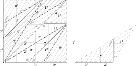
Figure 7.1. The map $\hat{T}$, $\lambda=1/\gamma$. ($\ell^{k}$ stands for $T^{k}(D_{\ell})$.)

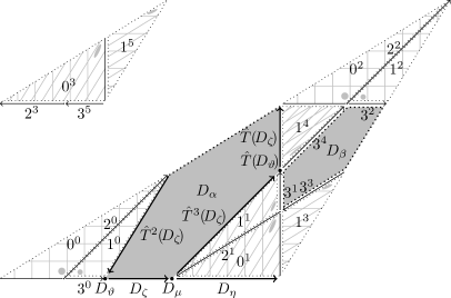
Figure 7.2. The trajectory of the scaled domains and $\mathcal{P}$, $\lambda=1/\gamma$. ($\ell^{k}$ stands for $\hat{T}^{k}U(D_{\ell})$.)

Theorem 7.1.

If $\lambda=1/\gamma$, then the minimal period length $\pi(z)$ is

$1$ if $z=(0,0)$ $2(5\cdot 4^{n}+4)/3$ if $S^{n}R(z)=\big{(}\frac{\gamma}{\gamma^{2}+1},\frac{1/\gamma}{\gamma^{2}+1}\big{)}$ for some $n\geq 0$ $10(5\cdot 4^{n}+4)/3$ for the other points with $S^{n}R(z)\in D_{\alpha}$ $4(5\cdot 4^{n}-2)/3$ if $S^{n}R(z)=\big{(}\frac{\gamma^{2}}{\gamma^{2}+1},\frac{1}{\gamma^{2}+1}\big{)}$ for some $n\geq 0$ $20(5\cdot 4^{n}-2)/3$ for the other points with $S^{n}R(z)\in D_{\beta}$ $5(4^{n+1}-1)/3$ if $S^{n}R(z)=(0,1/2)$ for some $n\geq 0$ $10(4^{n+1}-1)/3$ for the other points with $S^{n}R(z)\in D_{\vartheta}$ $5(2\cdot 4^{n+1}+7)/3$ if $S^{n}R(z)=\hat{T}^{m}(1/(2\gamma),0)$ for some $m\in\{0,1,2,3\}$ and $n\geq 0$ $10(2\cdot 4^{n+1}+7)/3$ for the other points with $S^{n}R(z)\in\hat{T}^{m}(D_{\zeta})$ $(10\cdot 4^{n}+11)/3$ if $S^{n}R(z)=(1/\gamma^{2},0)$ for some $n\geq 0$ $(5\cdot 4^{n+1}+19)/3$ if $S^{n}R(z)=\hat{T}^{m}(1/\gamma^{3},0)$ for some $m\in\{0,1\}$ and $n\geq 0$ $\infty$ if $S^{n}R(z)\in\mathcal{D}\setminus\mathcal{P}$ for all $n\geq 0$.

Proof.

As for $\lambda=-1/\gamma$, we have

$$\begin{pmatrix}|\sigma^{n}(0)|_{0}\\ |\sigma^{n}(0)|_{1}\end{pmatrix}=4^{n}\begin{pmatrix}1/3\\ 1/3\end{pmatrix}+\begin{pmatrix}2/3\\ -1/3\end{pmatrix},\qquad\begin{pmatrix}|\sigma^{n}(1)|_{0}\\ |\sigma^{n}(1)|_{1}\end{pmatrix}=4^{n}\begin{pmatrix}2/3\\ 2/3\end{pmatrix}+\begin{pmatrix}-2/3\\ 1/3\end{pmatrix},$$

hence $\tau(\sigma^{n}(0))=\frac{10}{3}4^{n}+\frac{8}{3}$, $\tau(\sigma^{n}(1))=\frac{20}{3}4^{n}-\frac{8}{3}$, $\tau(\sigma^{n}(2))=\frac{10}{3}4^{n}+\frac{11}{3}$, $\tau(\sigma^{n}(3))=\frac{20}{3}4^{n}-\frac{5}{3}$. For $S^{n}R(z)\in D_{\alpha}$, we have $\pi(z)=\tau(\sigma^{n}(0))$ and $\pi(z)=5\tau(\sigma^{n}(0))$ respectively; if $S^{n}R(z)\in D_{\beta}$, then $\pi(z)=\tau(\sigma^{n}(1))$ and $5\tau(\sigma^{n}(1))$ respectively; if $S^{n}R(z)\in D_{\eta}$, then $\pi(z)=\tau(\sigma^{n}(3))$ and $2\tau(\sigma^{n}(3))$ respectively; if $S^{n}R(z)\in D_{\zeta}$, then $\pi(z)=\tau(\sigma^{n}(0002))$ and $2\tau(\sigma^{n}(0002))$ respectively; if $S^{n}R(z)=\hat{T}^{m}(1/\gamma^{3},0)$, then $\pi(z)=\tau(\sigma^{n}(02))$; if $S^{n}R(z)=(1/\gamma^{2},0)$, then $\pi(z)=\tau(\sigma^{n}(2))$. ∎

Note that $\hat{T}^{m}U(D_{3})$ plays no role in the calculation of $\delta$ since $U(D_{3})\subset U(\mathcal{P})$ and thus $\pi(z)<\infty$ for all $z\in\hat{T}^{m}U(D_{3})$. For the other $z\in\mathcal{D}\setminus(\mathcal{P}\cup U(\mathcal{D}))$, we choose $\hat{s}(z)$ as follows:

$$z\in\hat{T}^{2}U(D_{0}\cup D_{1}\cup D_{2}):\ \hat{s}(z)=-2,\,s(z)=-10,\ t(z)=\hat{T}^{-2}(z)-z=(-1/\gamma,-1/\gamma^{2})$$

$$z\in\hat{T}U(D_{1}\cup D_{2}):\ \hat{s}(z)=-1,\,s(z)=-6,\ t(z)=\hat{T}^{-1}(z)+zA^{-1}=(1,1/\gamma)$$

$$z\in\hat{T}^{4}U(D_{1}):\ \hat{s}(z)=1,\,s(z)=6,\ t(z)=\hat{T}(z)+zA=(1/\gamma,0)$$

$$z\in\hat{T}U(D_{0})\cup\hat{T}^{3}U(D_{1}):\ \hat{s}(z)=2,\,s(z)=10,\ t(z)=\hat{T}^{2}(z)-z=(-1/\gamma^{2},0)$$

This gives again $\delta=\gamma^{2}/\gamma=\gamma$ since

$$\{(1/\gamma,0)A^{h}:\,h\in\mathbb{Z}\}=\pm\{(1/\gamma,0),\,(0,1/\gamma),\,(1/\gamma,1),\,(1,1),\,(1,1/\gamma)\}.$$

Theorem 7.2.

$\pi(z)$ is finite for all $z\in(\mathbb{Z}[\gamma]\cap[0,1))^{2}$, but $\big{(}T^{k}\big{(}1/4,1/(4\gamma^{3})\big{)}\big{)}_{k\in\mathbb{Z}}$ is aperiodic.

Proof.

Conjecture 1.1 holds for $\lambda=1/\gamma$ since no $z\in\mathbb{Z}[\gamma]^{2}\cap\mathcal{D}$ satisfies $\|z^{\prime}\|_{\infty}\leq\gamma$. It can be shown that all points in $(\frac{1}{2}\mathbb{Z}[\gamma]\cap[0,1))^{2}$ and $(\frac{1}{3}\mathbb{Z}[\gamma]\cap[0,1))^{2}$ are periodic as well. If $z=\big{(}1/4,1/(4\gamma^{3})\big{)}$, then we have $S(z)=\big{(}\gamma^{2}/4,1/(4\gamma)\big{)}$, $S^{2}(z)=\gamma^{2}\big{(}S(z)-(1/\gamma^{2},0)\big{)}=\big{(}(3\gamma-2)/4,\gamma/4\big{)}$ and $S^{3}(z)=\gamma^{2}\big{(}S^{2}(z)-(1/\gamma,1/\gamma^{2})\big{)}=\big{(}1/4,1/(4\gamma^{3})\big{)}=z$. ∎

Figure 7.3. Aperiodic points, $\lambda=1/\gamma$.

Figure 7.4. Aperiodic points, $\lambda=-\gamma$.

8. The case $\lambda=-\gamma=-2\cos\frac{\pi}{5}$

Let $\lambda=-\gamma$ ($\lambda^{\prime}=1/\gamma$) and set

$$\mathcal{D}=\{(x,y)\in[0,1)^{2}:\,x<y,\,\gamma x+y\geq 4-\gamma\}=D_{0}\cup D_{1}$$

with $D_{0}=\{(x,y)\in\mathcal{D}:x>1-1/\gamma^{5}\}$, $D_{1}=\{(x,y)\in\mathcal{D}:x\leq 1-1/\gamma^{5}\}$. Figure 8.1 shows that $\hat{T}(z)=T^{\tau(\ell)}(z)$ if $z\in D_{\ell}$, with $\tau(0)=42$, $\tau(1)=28$, and

$$\mathcal{R}=\{(0,0)\}\cup D_{A}\cup D_{B}\cup\bigcup\nolimits_{k=0}^{4}T^{k}(D_{\Gamma})\cup\bigcup\nolimits_{k=0}^{1}T^{k}(D_{\Delta})\cup\bigcup\nolimits_{k=0}^{24}T^{k}(D_{E})\cup\bigcup\nolimits_{k=0}^{10}T^{k}(D_{Z})$$

with $D_{A}=\{z:T^{k+1}(z)=T^{k}(z)A+(0,1)\mbox{ for all }k\in\mathbb{Z}\}$, $D_{B}=\{z:T^{k+1}(z)=T^{k}(z)A+(0,2)\}$, $D_{\Delta}=\{z\in[0,1)^{2}:T^{2k+1}(z)=T^{2k}(z)A+(0,2),\,T^{2k}(z)=T^{2k-1}(z)A+(0,1)\mbox{ for all }k\in\mathbb{Z}\}$, $D_{\Gamma}=\{(x,y):0\leq x,y\leq 1/\gamma^{4}\}\setminus\{(0,0),(1/\gamma^{4},1/\gamma^{4})\}$, $D_{E}=\{(x,x):1-1/\gamma^{5}<x<1\}$, $D_{Z}=\{(1-1/\gamma^{5},1-1/\gamma^{5})\}$. Set $\kappa=1/\gamma^{2}$, $V(z)=\gamma^{4}\big{(}(1,1)-z)$, i.e.

$$U(z)=(1,1)-\big{(}(1,1)-z\big{)}/\gamma^{2}=z/\gamma^{2}+(1/\gamma,1/\gamma).$$

Then Figure 8.2 shows that the conditions in Section 3 are satisfied by $\varepsilon=1$ and

$$\sigma:\ 0\mapsto 010\qquad 1\mapsto 01110.$$

All points in $\mathcal{P}=D_{\alpha}\cup D_{\beta}$ are periodic, with $D_{\alpha}=\{z\in\mathcal{D}:\hat{T}^{k}(z)\in D_{0}\mbox{ for all }k\in\mathbb{Z}\}$, $D_{\beta}=\{z\in\mathcal{D}:\hat{T}^{k}(z)\in D_{1}\mbox{ for all }k\in\mathbb{Z}\}$. Since $|\sigma^{n}(\ell)|\to\infty$ as $n\to\infty$ for all $\ell\in\mathcal{A}$, all conditions of Proposition 3.3 and Theorem 3.4 are satisfied, and we obtain the following theorem.

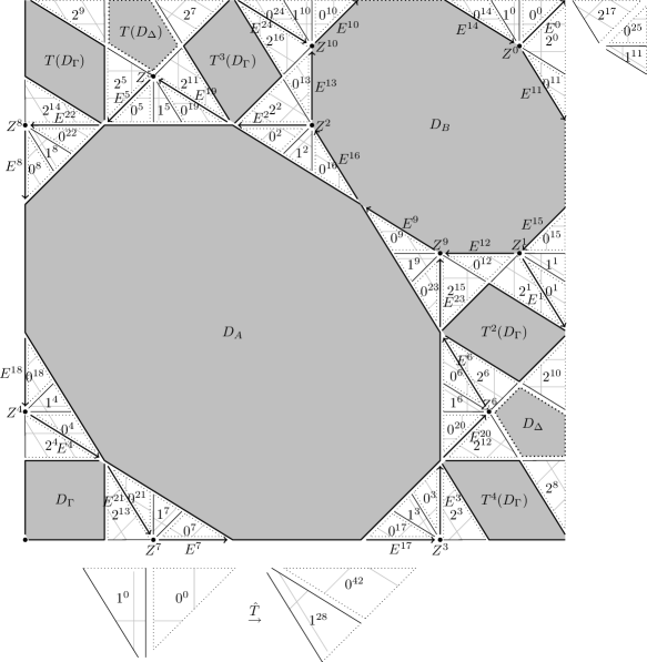
Figure 8.1. The map $\hat{T}$ and the set $\mathcal{R}$, $\lambda=-\gamma$. ($\ell^{k}$ stands for $T^{k}(D_{\ell})$.)

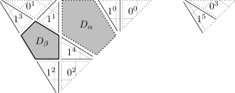
Figure 8.2. The trajectory of the scaled domains and $\mathcal{P}$, $\lambda=-\gamma$. ($\ell^{k}$ stands for $\hat{T}^{k}U(D_{\ell})$.)

Theorem 8.1.

If $\lambda=-\gamma$, then the minimal period length $\pi(z)$ is

$1$ if $z\in\{(0,0),(1/\gamma^{2},1/\gamma^{2}),(2/\gamma^{2},2/\gamma^{2})\}$ $2$ if $z\in\{(\frac{5-\gamma}{\gamma^{2}+1},\frac{2/\gamma^{2}}{\gamma^{2}+1}),(\frac{2/\gamma^{2}}{\gamma^{2}+1},\frac{5-\gamma}{\gamma^{2}+1})\}$ $5$ if $z=T^{m}(1/(2\gamma^{4}),1/(2\gamma^{4}))$ for some $m\in\{0,1,2,3,4\}$ $10$ for the other points of $D_{A}$, $D_{B}$, $T^{m}(D_{\Gamma})$, $T^{m}(D_{\Delta})$ $11$ if $z=T^{m}(1-1/\gamma^{5},1-1/\gamma^{5})$ for some $m\in\{0,1,\ldots,10\}$ $25$ if $z=T^{m}(1-1/(2\gamma^{5}),1-1/(2\gamma^{5}))$ for some $m\in\{0,1,\ldots,24\}$ $50$ for the other points of $T^{m}(D_{E})$ $2(35\cdot 4^{n}+28)/3$ if $S^{n}R(z)$ is the center of $D_{\alpha}$ $10(35\cdot 4^{n}+28)/3$ for the other points of $D_{\alpha}$ $4(35\cdot 4^{n}-14)/3$ if $S^{n}R(z)$ is the center of $D_{\beta}$ $20(35\cdot 4^{n}-14)/3$ for the other points of $D_{\beta}$ $\infty$ if $S^{n}R(z)\in\mathcal{D}\setminus\mathcal{P}$ for all $n\geq 0$

Proof.

As for $\lambda=-1/\gamma$ and $\lambda=1/\gamma$, we have

$$\begin{pmatrix}|\sigma^{n}(0)|_{0}\\ |\sigma^{n}(0)|_{1}\end{pmatrix}=4^{n}\begin{pmatrix}1/3\\ 1/3\end{pmatrix}+\begin{pmatrix}2/3\\ -1/3\end{pmatrix},\qquad\begin{pmatrix}|\sigma^{n}(1)|_{0}\\ |\sigma^{n}(1)|_{1}\end{pmatrix}=4^{n}\begin{pmatrix}2/3\\ 2/3\end{pmatrix}+\begin{pmatrix}-2/3\\ 1/3\end{pmatrix},$$

hence $\tau(\sigma^{n}(0))=(70\cdot 4^{n}+56)/3$, $\tau(\sigma^{n}(1))=(140\cdot 4^{n}-56)/3$. For $S^{n}R(z)\in D_{\alpha}$, we have $\pi(z)=\tau(\sigma^{n}(0))$ and $5\tau(\sigma^{n}(0))$ respectively; if $S^{n}R(z)\in D_{\beta}$, then $\pi(z)=\tau(\sigma^{n}(1))$ and $5\tau(\sigma^{n}(1))$ respectively. ∎

We choose $\hat{s}(z)$ as follows and obtain the following $s(z),t(z)$:

$$z\in\hat{T}^{2}U(D_{0}\cup D_{1}):\ \hat{s}(z)=-2,\,s(z)=-70,\ t(z)=V(\hat{T}^{-2}(z))-V(z)=(-1/\gamma^{2},-1/\gamma^{2})$$

$$z\in\hat{T}U(D_{1}):\ \hat{s}(z)=-1,\,s(z)=-42,\ t(z)=V(\hat{T}^{-1}(z))-V(z)A^{-2}=(1/\gamma,1/\gamma)$$

$$z\in\hat{T}^{4}U(D_{1}):\ \hat{s}(z)=1,\,s(z)=42,\ t(z)=V(\hat{T}(z))-V(z)A^{2}=(1,0)$$

$$z\in\hat{T}U(D_{0})\cup\hat{T}^{3}U(D_{1}):\ \hat{s}(z)=2,\,s(z)=70,\ t(z)=V(\hat{T}^{2}(z))-V(z)=(-1/\gamma,0)$$

This gives again $\delta=\gamma^{2}/\gamma=\gamma$ since

$$\{(1,0)A^{h}:\,h\in\mathbb{Z}\}=\pm\{(1,0),\,(0,1),\,(1,-1/\gamma),\,(1/\gamma,1/\gamma),\,(1/\gamma,-1)\}.$$

Theorem 8.2.

$\pi(z)$ is finite for all $z\in(\mathbb{Z}[\gamma]\cap[0,1))^{2}$, but $\pi\big{(}1-1/(3\gamma^{2}),1-1/(3\gamma^{5})\big{)}=\infty$.

Proof.

Since $V(\mathcal{D})=\{(x,y):x>y>0,\gamma x+y\leq\gamma\}$, we have no point $z\in\mathbb{Z}[\gamma]^{2}\cap\mathcal{D}$ with $\|V(z)^{\prime}\|_{\infty}\leq\gamma$, and Conjecture 1.1 holds for $\lambda=-\gamma$. If $V(z)=\big{(}\gamma^{2}/3,1/(3\gamma)\big{)}$, then we have

$$VS(z)=\gamma^{2}\Big{(}V(z)-\Big{(}\frac{1}{\gamma},0\Big{)}\Big{)}=\Big{(}\frac{2}{3},\frac{\gamma}{3}\Big{)},\ VS^{2}(z)=\gamma^{2}\Big{(}VS(z)-\Big{(}\frac{1}{\gamma^{2}},\frac{1}{\gamma^{2}}\Big{)}\Big{)}=\Big{(}\frac{\gamma^{2}+1}{3\gamma},\frac{2}{3\gamma}\Big{)},$$

$VS^{3}(z)=\gamma^{2}\big{(}VS^{2}(z)-\big{(}\frac{1}{\gamma^{2}},\frac{1}{\gamma^{2}}\big{)}\big{)}=\big{(}\frac{3\gamma-2}{3},\frac{1}{3\gamma^{3}}\big{)}$ and $VS^{4}(z)=\gamma^{2}\big{(}VS^{3}(z)-\big{(}\frac{1}{\gamma},0\big{)}\big{)}=V(z)$. ∎

9. The case $\lambda=\sqrt{3}=-2\cos\frac{5\pi}{6}$

Figure 9.1. The first return map on $\mathcal{D}_{1}$ and $\mathcal{D}_{2}$ respectively, $\lambda=\sqrt{3}$. ($\ell^{k}$ stands for $T^{k}(D_{\ell})$.)

The case $\lambda=\sqrt{3}$ is much more involved than the previous cases. Therefore we show only that all points in $(\mathbb{Z}[\sqrt{3}]\cap[0,1))^{2}$ are periodic and refrain from calculating the period lengths. Furthermore we postpone the determination of $\hat{T}$ and $\mathcal{R}$ to Appendix A. Let

$$\mathcal{D}=\{(x,y):2x-\sqrt{3}y<2-\sqrt{3},2y-\sqrt{3}x<2-\sqrt{3},y-\sqrt{3}x<195-113\sqrt{3},x-\sqrt{3}y<195-113\sqrt{3}\}$$

and $\mathcal{D}_{1}=\mathcal{D}\setminus\mathcal{D}_{2}$, where $\mathcal{D}_{2}$ is defined by the inequalities

$$2x-\sqrt{3}y>267-154\sqrt{3},\,2y-\sqrt{3}x>267-154\sqrt{3},\,y-\sqrt{3}x>98-57\sqrt{3},\,x-\sqrt{3}y>98-57\sqrt{3}.$$

The sets $\mathcal{D}_{1}$ and $\mathcal{D}_{2}$ have to be treated separately because their trajectories are disjoint, and both sets contain aperiodic points. The trajectories of aperiodic points in $\mathcal{D}_{1}$ come arbitrarily close to $(1,1)$, whereas $(72-41\sqrt{3},72-41\sqrt{3})$ is a limit point in $\mathcal{D}_{2}$. (Note that $72-41\sqrt{3}=1-(\sqrt{3}+1)(2-\sqrt{3})^{4}\approx 0.9859$.) The scaling maps are

$$U_{1}(z) =(2-\sqrt{3})z+(\sqrt{3}-1,\sqrt{3}-1)=V_{1}^{-1}(\kappa V_{1}(z))\qquad\mbox{for }z\in\mathcal{D}_{1},$$

$$U_{2}(z) =(2-\sqrt{3})z+(113\sqrt{3}-95,113\sqrt{3}-195)=V_{2}^{-1}(\kappa V_{2}(z))\qquad\mbox{for }z\in\mathcal{D}_{2},$$

with $\kappa=2-\sqrt{3}$, $V_{1}(z)=\big{(}(1,1)-z\big{)}/\kappa^{4}$, $V_{2}(z)=\big{(}z-(72-41\sqrt{3},72-41\sqrt{3})\big{)}/\kappa^{5}$. Then we have

$$V_{1}(\mathcal{D}) =\{(x,y):2x>\sqrt{3}y,\,2y>\sqrt{3}x,\,x>\sqrt{3}y-2,\,y>\sqrt{3}x-2\},$$

$$V_{2}(\mathcal{D}_{2}) =\{(x,y):2x>\sqrt{3}y,\,2y>\sqrt{3}x,\,x>\sqrt{3}y-2-\sqrt{3},\,y>\sqrt{3}x-2-\sqrt{3}\}.$$

The first return map $\hat{T}$ induces a partition of $\mathcal{D}_{1}$ into sets $D_{0},\ldots,D_{9}$ and a partition of $\mathcal{D}_{2}$ into sets $D_{\mathbf{0}},\ldots,D_{\mathbf{4}}$, as in Figure 9.1. These sets are defined by the following (in)equalities:

$$\begin{array}[]{c|c|c|c|c}V_{1}(D_{0})&V_{1}(D_{1})&V_{1}(D_{2})&V_{1}(D_{3})&V_{1}(D_{4})\\ \hline\cr x>\sqrt{3}y-1&x>\sqrt{3}y-1&2x>\sqrt{3}y+\sqrt{3}-1&2y>\sqrt{3}x+\sqrt{3}-1&2y>\sqrt{3}x+\sqrt{3}-1\\ &x<2&x>2&x>2,\ y<2\sqrt{3}-1&y>2\sqrt{3}-1\end{array}$$

$$\begin{array}[]{c|c|c|c|c}V_{1}(D_{5})&V_{1}(D_{6})&V_{1}(D_{7})&V_{1}(D_{8})&V_{1}(D_{9})\\ \hline\cr x=\sqrt{3}y-1&x=2&y=2\sqrt{3}-1&2x=\sqrt{3}y+\sqrt{3}-1&2y=\sqrt{3}x+\sqrt{3}-1\\ &&x<3-1/\sqrt{3}&x>2&x>2\end{array}$$

$$\begin{array}[]{c|c|c|c|c}V_{2}(D_{\mathbf{0}})&V_{2}(D_{\mathbf{1}})&V_{2}(D_{\mathbf{2}})&V_{2}(D_{\mathbf{3}})&V_{2}(D_{\mathbf{4}})\\ \hline\cr y>\sqrt{3}x-1&y<\sqrt{3}x-1,\,x<\sqrt{3}+1&x>\sqrt{3}+1&y=\sqrt{3}x-1&x=\sqrt{3}+1\end{array}$$

The return times of $z\in D_{\ell}$ to $\mathcal{D}$ are given by the following tables.

$$\begin{array}[]{c|c|c|c|c|c|c|c|c|c}D_{0}&D_{1}&D_{2}&D_{3}&D_{4}&D_{5}&D_{6}&D_{7}&D_{8}&D_{9}\\ \hline\cr 1601,\,1733&3175,\,3307&3230&7406&9771&3021&3593&9799&11473&7907\end{array}$$

$$\begin{array}[]{c|c|c|c|c}D_{\mathbf{0}}&D_{\mathbf{1}}&D_{\mathbf{2}}&D_{\mathbf{3}}&D_{\mathbf{4}}\\ \hline\cr 19459&15524&3175,\,3307&18171&3593\end{array}$$

Note that the return times are not constant on all $D_{\ell}$. E.g., the return time for $z\in D_{0}$ is $1601$ if $V_{1}(z)=(1,y)$ and $1733$ else, see Appendix A for details. Since we do not calculate the period lengths, it is not necessary to distinguish between the parts of $D_{\ell}$ with different period lengths.

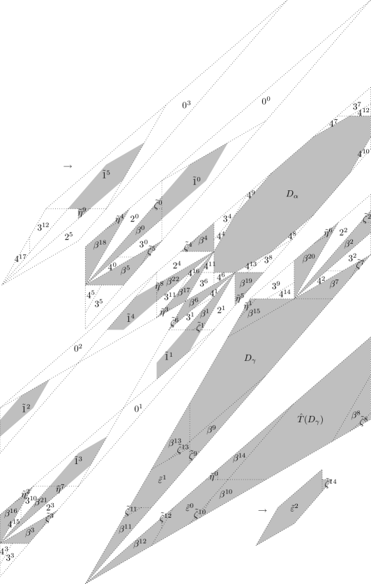
Figure 9.2. The trajectory of the open scaled sets in $\mathcal{D}_{1}$ and the set $\mathcal{P}_{1}$, $\lambda=\sqrt{3}$.
($\ell^{k}$ stands for $\hat{T}^{k}U_{1}(D_{\ell})$ if $\ell\in\{0,\tilde{1},2,3,4\}$, for $\hat{T}^{k}(D_{\ell})$ else.)

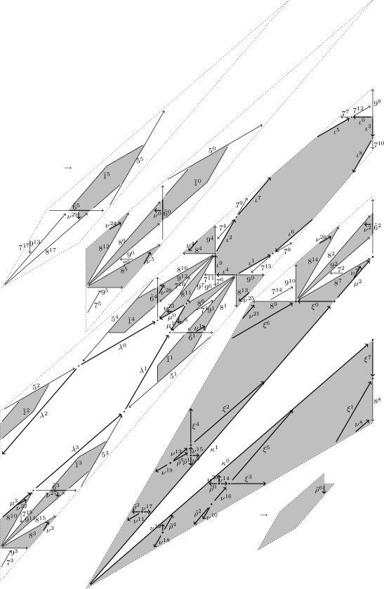
Figure 9.3. The trajectory of the scaled lines and the set $\mathcal{P}_{1}$, $\lambda=\sqrt{3}$.
($\ell^{k}$ stands for $\hat{T}^{k}U_{1}(D_{\ell})$ if $\ell\in\{\bar{1},5,\tilde{6},7,8,9\}$, for $\hat{T}^{k}(D_{\ell})$ else.)

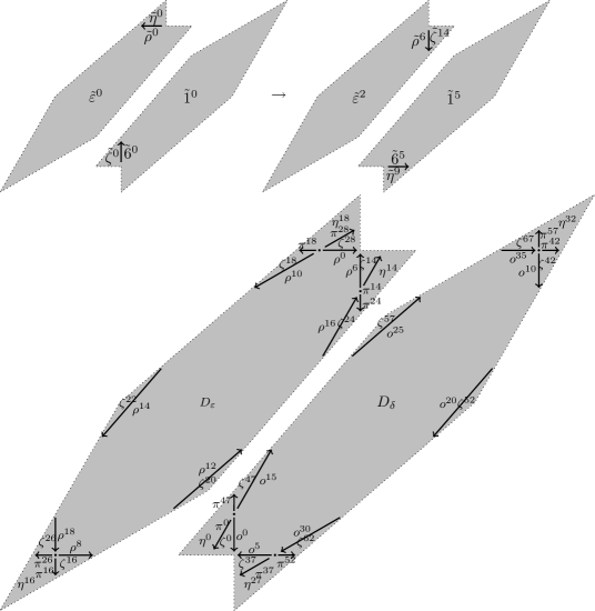
Figure 9.4. Small parts of $\mathcal{P}_{1}$, $\lambda=\sqrt{3}$. ($\ell^{k}$ stands for $\hat{T}^{k}(D_{\ell})$ for $\ell\not\in\{\tilde{1},\tilde{6}\}$.)

9.1. The scaling domain $\mathcal{D}_{1}$.

Figure 9.2 shows the trajectory of the open scaled sets in $\mathcal{D}_{1}$. Here, $V_{1}(\mathcal{D}_{1})$ is split up into the three stripes $x<\sqrt{3}-1$, $\sqrt{3}-1<x<2$ and $x>2$, and $D_{\tilde{1}}$ denotes the set given by $V_{1}(D_{\tilde{1}})=\{(x,y)\in V_{1}(\mathcal{D}):x>\sqrt{3}y-1,x<2\}$. We see that

$$\sigma_{1}:\begin{array}[]{rclrclrclrcl}0&\mapsto&010&3&\mapsto&012100001210&5&\mapsto&01510&7&\mapsto&01210000500001210\\ 1&\mapsto&01110&4&\mapsto&01210000000001210&6&\mapsto&01610&8&\mapsto&01210012621001210\\ 2&\mapsto&01210&&&&&&&9&\mapsto&0121005001210\end{array}$$

codes the trajectory of $U_{1}(D_{\ell})$, $\ell\in\{0,1,2,3,4\}$, with $\hat{T}^{|\sigma_{1}(\ell)|}U_{1}(z)=U_{1}\hat{T}(z)$ for $z\in D_{\ell}$. All points in $D_{\alpha}$, $D_{\beta}$ and $D_{\gamma}$ are periodic. Figure 9.4 shows that $D_{\tilde{\varepsilon}},D_{\tilde{\zeta}},D_{\tilde{\eta}}$ and the grey part of $U_{1}(\mathcal{D}_{\tilde{1}})$ split up further, but all their points are periodic as well.

The trajectory of the scaled lines is depicted in Figure 9.3, where again $V_{1}(\mathcal{D}_{1})$ is split up into the stripes $x<\sqrt{3}-1$, $\sqrt{3}-1\leq x<2$ and $x\geq 2$. Here, $D_{\bar{1}}$ denotes boundary lines of $D_{1}$, and $D_{\tilde{6}}$ is given by $V_{1}(D_{\tilde{6}})=\{(2,y)\in V_{1}(\mathcal{D})\}$. We see that $\sigma_{1}$ codes the trajectory of $U_{1}(D_{\ell})$, $\ell\in\{5,6,7,8,9\}$, as well and satisfies the conditions in Section 3 (with respect to $\mathcal{D}_{1}$). All points in $D_{\iota},D_{\kappa},D_{\lambda},D_{\mu},D_{\nu},D_{\xi},D_{o},D_{\pi},D_{\rho}$ (and their orbits) are periodic. The finitely many remaining points in $\mathcal{P}_{1}=\{z\in\mathcal{D}_{1}:\hat{T}^{m}(z)\not\in U_{1}(\mathcal{D}_{1})\mbox{ for all }m\in\mathbb{Z}\}$ are clearly periodic as well. Since $|\sigma_{1}^{n}(\ell)|\to\infty$ for all $\ell\in\{0,\ldots,9\}$, we can use Proposition 3.5 to show the following proposition.

Proposition 9.1.

$\pi(z)$ is finite for all $z\in\mathbb{Z}[\sqrt{3}]^{2}\cap\mathcal{D}_{1}$, but $\pi(V_{1}^{-1}(\sqrt{3}+1/4,7/4))=\infty$.

Proof.

First we show that only $D_{0}$ and $D_{1}$ contain aperiodic points: $D_{3},D_{4},D_{7},D_{8},D_{9}$ lie in $\mathcal{P}_{1}$. The only part of $D_{2}$ which is not in $\mathcal{P}_{1}$ or $\hat{T}^{m}U_{1}(\mathcal{P}_{1})$, lies in $\hat{T}^{2}U_{1}(D_{2})$. By iterating this argument on $\hat{T}^{2}U_{1}(D_{2})$, the possible set of aperiodic points in $D_{2}$ becomes smaller and smaller, and converges to $V_{1}^{-1}(2,\sqrt{3})\not\in D_{2}$. A similar reasoning shows that all points in $D_{5}$ and $D_{6}$ are periodic. Therefore it is sufficient to determine $t(z)$ for points in the trajectories of $U_{1}(D_{0}\cup D_{1})$.

$$z\in\hat{T}U_{1}(D_{0})\cup\hat{T}^{3}U_{1}(D_{1}):\ \hat{s}(z)=2,\,s(z)\equiv 0\bmod 12,\,t(z)=(1-\sqrt{3})(\sqrt{3},2)$$

$$z\in\hat{T}^{4}U_{1}(D_{1}):\ \hat{s}(z)=1,\,s(z)\equiv 5\bmod 12,\,t(z)=V_{1}(\hat{T}(z))-V_{1}(z)A^{5}=(\sqrt{3},2)$$

$$z\in\hat{T}U_{1}(D_{1}):\ \hat{s}(z)=-1,\,s(z)\equiv-5\bmod 12,\,t(z)=(2,\sqrt{3})$$

$$z\in\hat{T}^{2}U_{1}(D_{0})\cup\hat{T}^{2}U_{1}(D_{1}):\ \hat{s}(z)=-2,\,s(z)\equiv 0\bmod 12,\,t(z)=(1-\sqrt{3})(2,\sqrt{3})$$

We have $\delta_{1}=(\sqrt{3}+1)2/(\sqrt{3}+1)=2$ since

$$\{(\sqrt{3},2)A^{h}:\,h\in\mathbb{Z}\}=\pm\{(\sqrt{3},2),\,(2,\sqrt{3}),\,(\sqrt{3},1),\,(1,0),\,(0,1),\,(1,\sqrt{3})\}.$$

The only point $z\in V_{1}(\mathbb{Z}[\sqrt{3}]^{2}\cap\mathcal{D}_{1})$ with $\|z^{\prime}\|_{\infty}\leq 2$ is $(1,1)\in V_{1}(D_{\alpha})$.

If $V_{1}(z)=(\sqrt{3}+1/4,7/4)$, then we have

$$V_{1}S(z) =(2+\sqrt{3})\big{(}V_{1}(z)+(1-\sqrt{3})(2,\sqrt{3})\big{)}=(3/2+\sqrt{3}/4,3\sqrt{3}/4+1/2),$$

$$V_{1}S^{2}(z) =(2+\sqrt{3})\big{(}V_{1}S(z)+(1-\sqrt{3})(2,\sqrt{3})\big{)}=(7/4,\sqrt{3}+1/4),$$

$V_{1}S^{3}(z)=(2+\sqrt{3})\big{(}V_{1}S^{2}(z)+(1-\sqrt{3})(\sqrt{3},2)\big{)}=(3\sqrt{3}/4+1/2,3/2+\sqrt{3}/4)$, $V_{1}S^{4}(z)=V_{1}(z)$. ∎

Remark. The primitive part of $\sigma_{1}$ is again $0\mapsto 010$, $1\mapsto 01110$.

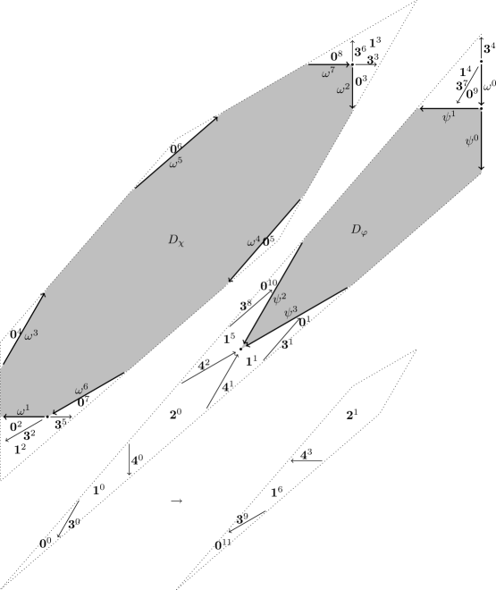
Figure 9.5. The trajectory of the scaled domains in $\mathcal{D}_{2}$ and the set $\mathcal{P}_{2}$, $\lambda=\sqrt{3}$.
($\ell^{k}$ stands for $\hat{T}^{k}(D_{\ell})$ if $\ell\in\{\psi,\omega\}$, for $\hat{T}^{k}U_{2}(D_{\ell})$ else.)

9.2. The scaling domain $\mathcal{D}_{2}$

Figure 9.5 shows the trajectory of the the scaled domains in $\mathcal{D}_{2}$. Here, $V_{2}(\mathcal{D}_{2})$ is split up into $x\leq\sqrt{3}+1$ and $x>\sqrt{3}+1$. With $\varepsilon_{2}=1$ and

$$\sigma_{2}:\begin{array}[]{rclrcl}\mathbf{0}&\mapsto&\mathbf{0}\mathbf{1}\mathbf{2}\mathbf{2}\mathbf{2}\mathbf{2}\mathbf{2}\mathbf{2}\mathbf{2}\mathbf{1}\mathbf{0}&\mathbf{3}&\mapsto&\mathbf{0}\mathbf{1}\mathbf{2}\mathbf{2}\mathbf{4}\mathbf{2}\mathbf{2}\mathbf{1}\mathbf{0}\\ \mathbf{1}&\mapsto&\mathbf{0}\mathbf{1}\mathbf{2}\mathbf{2}\mathbf{1}\mathbf{0}&\mathbf{4}&\mapsto&\mathbf{0}\mathbf{3}\mathbf{0}\\ \mathbf{2}&\mapsto&\mathbf{0}\end{array}$$

the conditions in Section 3 are satisfied. The set $\mathcal{P}_{2}=\{z\in\mathcal{D}_{2}:\hat{T}^{m}(z)\not\in U_{2}(\mathcal{D}_{2})\mbox{ for all }m\in\mathbb{Z}\}$ consists of the orbits of $D_{\varphi},D_{\chi},D_{\psi},D_{\omega}$ and several isolated (periodic) points. Since $|\sigma_{2}^{n}(\ell)|\to\infty$ for all $\ell\in\{\mathbf{0},\mathbf{1},\mathbf{2},\mathbf{3},\mathbf{4}\}$, we can use Proposition 3.5 to show the following proposition.

Proposition 9.2.

$\pi(z)$ is finite for all $z\in\mathbb{Z}[\sqrt{3}]^{2}\cap\mathcal{D}_{2}$, but $\pi(V_{2}^{-1}(5/7,3\sqrt{3}/7))=\infty$.

Proof.

Similarly to $\mathcal{D}_{1}$, we see that all points in $D_{\mathbf{3}}$ and $D_{\mathbf{4}}$ are periodic. Choose $\hat{s}(z)$ as follows:

$$z\in\hat{T}^{10}U_{2}(D_{\mathbf{0}})\cup\hat{T}^{5}U_{2}(D_{\mathbf{1}}):\ \hat{s}(z)=1,\,s(z)\equiv 7\bmod 12,\,t(z)=(2,\sqrt{3})$$

$$z\in\hat{T}^{9}U_{2}(D_{\mathbf{0}})\cup\hat{T}^{4}U_{2}(D_{\mathbf{1}}):\ \hat{s}(z)=2,\,s(z)\equiv 3\bmod 12,\,t(z)=(1-\sqrt{3},\sqrt{3}-1)$$

$$z\in\hat{T}^{8}U_{2}(D_{\mathbf{0}})\cup\hat{T}^{3}U_{2}(D_{\mathbf{1}}):\ \hat{s}(z)=3,\,s(z)\equiv 10\bmod 12,\,t(z)=(1-\sqrt{3},-3)$$

$$z\in\hat{T}^{7}U_{2}(D_{\mathbf{0}}):\ \hat{s}(z)=4,\,s(z)\equiv 5\bmod 12,\,t(z)=\sqrt{3}(\sqrt{3},2)$$

$$z\in\hat{T}^{6}U_{2}(D_{\mathbf{0}}):\ \hat{s}(z)=5,\,s(z)\equiv 0\bmod 12,\,t(z)=-2(\sqrt{3},2)$$

For the remaining $z\in\hat{T}^{m}U_{2}(D_{\mathbf{0}}\cup D_{\mathbf{1}})$, $\hat{s}(z),s(z)$ and $t(z)$ are obtained by symmetry. The sets $\{(1-\sqrt{3},\sqrt{3}-1)A^{h}:h\in\mathbb{Z}\}$ and $\{(\sqrt{3}-1,3)A^{h}:h\in\mathbb{Z}\}$ are

$$\pm\{(1-\sqrt{3},\sqrt{3}-1),(\sqrt{3}-1,2),(2,\sqrt{3}+1),(\sqrt{3}+1,\sqrt{3}+1),(\sqrt{3}+1,2),(2,\sqrt{3}-1)\},$$

$$\pm\{(\sqrt{3}-1,3),(3,2\sqrt{3}+1),(2\sqrt{3}+1,3+\sqrt{3}),(3+\sqrt{3},2+\sqrt{3}),(2+\sqrt{3},\sqrt{3}),(\sqrt{3},1-\sqrt{3})\},$$

hence $\delta_{2}=4/(\sqrt{3}+1)=2(\sqrt{3}-1)$. The only $x\in\mathbb{Z}[\sqrt{3}]$ with $0<x<5$ and $|x^{\prime}|\leq 2(\sqrt{3}-1)$ are $1,1+\sqrt{3},2+\sqrt{3}$ and $3+\sqrt{3}$. Therefore the only $z\in V_{2}(\mathbb{Z}[\sqrt{3}]^{2}\cap\mathcal{D}_{2})$ with $\|z^{\prime}\|_{\infty}\leq 2(\sqrt{3}-1)$ are $(1,1)$, the center of $V_{2}U_{2}(D_{\chi})$, $(1+\sqrt{3},1+\sqrt{3})$, the center of $D_{\mathbf{4}}$, $(2+\sqrt{3},2+\sqrt{3})$, the center of $D_{\chi}$, and $(3+\sqrt{3},3+\sqrt{3})$, a fixed point of $\hat{T}^{3}$.

If $V_{2}(z)=(5/7,3\sqrt{3}/7)$, then we have $V_{2}S(z)=(2+\sqrt{3})V_{2}(z)$ and
$V_{2}S^{2}(z)=(2+\sqrt{3})\big{(}V_{2}S(z)A^{3}+(1-\sqrt{3},\sqrt{3}-1)\big{)}=(5/7,3\sqrt{3}/7)=V_{2}(z)$. ∎

By combining Propositions 9.1 and 9.2 and the fact that all points in $\mathcal{R}$ are periodic (see Appendix A), we obtain the following theorem.

Theorem 9.3.

Conjecture 1.1 holds for $\lambda=\sqrt{3}$.

Remark. The eigenvalues corresponding to the primitive part of $\sigma_{2}$ ($\ell\in\{\mathbf{0},\mathbf{1},\mathbf{2}\}$) are $5,-2$ and $1$.

Figure 9.6. Aperiodic points, $\lambda=\sqrt{3}$.

Figure 9.7. Aperiodic points in $\mathcal{D}_{1}\cup\mathcal{D}_{2}$, $\lambda=\sqrt{3}$.

10. The case $\lambda=-\sqrt{3}=-2\cos\frac{\pi}{6}$

Figure 10.1. The map $\hat{T}$ on $\mathcal{D}$, $\lambda=-\sqrt{3}$. ($\ell^{k}$ stands for $T^{k}(D_{\ell})$.)

Let $\mathcal{D}=\{(x,y)\in[0,1)^{2}:x+\sqrt{3}y>5\sqrt{3}-6\mbox{ or }y+\sqrt{3}x>5\sqrt{3}-6\}$, $U_{1}$ as in Section 9 and

$$U(z)=U_{1}^{2}(z)=(2-\sqrt{3})^{2}z+(4\sqrt{3}-6,4\sqrt{3}-6)=V^{-1}(\kappa V(z)),$$

$\kappa=(2-\sqrt{3})^{2}$, $V(z)=\big{(}(1,1)-z\big{)}/\kappa$. Then we have

$$V(\mathcal{D})=\{(x,y):\ x>0,\ y>0,\ x+\sqrt{3}y<1\mbox{ or }y+\sqrt{3}x<1\}.$$

Figure 10.1 shows the first return map $\hat{T}$ on $\mathcal{D}$, which is determined in Appendix B. The sets $D_{0},\ldots,D_{6}$ satisfy the (in)equalities

$$\begin{array}[]{c|c|c}V(D_{0})&V(D_{1})&V(D_{2})\\ \hline\cr\sqrt{3}x+y<1&\sqrt{3}x+y>1,\,x<\sqrt{3}-1&x>\sqrt{3}-1,\,2x+\sqrt{3}y\neq\sqrt{3}\\ \end{array}$$

$$\begin{array}[]{c|c|c|c}V(D_{3})&V(D_{4})&V(D_{5})&V(D_{6})\\ \hline\cr\sqrt{3}x+y=1,\,x<1/2&\sqrt{3}x+y=1,\,x>1/2&x=\sqrt{3}-1&2x+\sqrt{3}y=\sqrt{3}\end{array}$$

The remaining point $z=V^{-1}(1/2,1-\sqrt{3}/2)$ has return time $183$ and satisfies $\hat{T}^{10}(z)=z$.

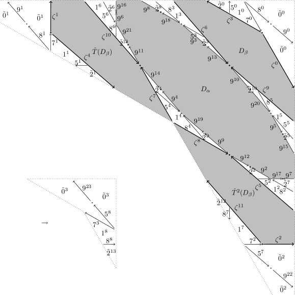
Figure 10.2. Trajectory of $U_{1}(\mathcal{D})$ and large parts of $\mathcal{P}$, $\lambda=-\sqrt{3}$. ($\ell^{k}$ stands for $\hat{T}^{k}U_{1}(D_{\ell})$.)

Figure 10.3. Trajectory of $U(\mathcal{D})$ and small parts of $\mathcal{P}$, $\lambda=-\sqrt{3}$. ($\ell^{k}$ stands for $\hat{T}^{k}U(D_{\ell})$.)

Figure 10.2 shows that the first return map on $U_{1}(\mathcal{D})$ differs from $U_{1}\hat{T}U_{1}^{-1}$ on several lines. Therefore we add the lines $D_{7},D_{8},D_{9}$ satisfying the following (in)equalities

$$\begin{array}[]{c|c|c}V(D_{7})&V(D_{8})&V(D_{9})\\ \hline\cr\sqrt{3}x+y=1&\sqrt{3}x+2y=1,\,x>2-\sqrt{3}&\sqrt{3}x+2y=1,\,x<2-\sqrt{3}\end{array}$$

and define $D_{\tilde{0}}=D_{0}\setminus V^{-1}(\{(x,y):\sqrt{3}x+2y=1\})$, $D_{\tilde{2}}=D_{2}\cup D_{6}$. For $z\in D_{\tilde{\ell}}$, $\ell\in\{0,2\}$ and $z\in D_{\ell}$, $\ell=1$, we have $\hat{T}^{|\sigma_{1}(\ell)|}U_{1}(z)=U_{1}\hat{T}(z)$ with

$$\sigma_{1}:\begin{array}[]{rclrclrclrcl}0&\mapsto&020&1&\mapsto&010^{4}10&2&\mapsto&010^{9}10&&&\\ 5&\mapsto&010^{4}40&7&\mapsto&050&8&\mapsto&060^{4}10&9&\mapsto&060^{9}30^{9}40\end{array}$$

Figure 10.3 shows that the substitution $\sigma$ given by $\sigma(\ell)=\sigma_{1}\sigma_{2}(\ell)$ with

$$\sigma_{2}:\begin{array}[]{rclrclrclrcl}0&\mapsto&020&1&\mapsto&010^{4}10&2&\mapsto&010^{9}10&&&\\ 3&\mapsto&050^{5}90^{5}80&4&\mapsto&050^{4}10&5&\mapsto&010^{4}70^{4}10&6&\mapsto&010^{4}80\end{array}$$

satisfies the conditions in Section 3 (with $\varepsilon=1$). The coding of the return path of the remaining point is $\sigma_{1}(050^{4}70^{4}80)$.

Theorem 10.1.

$\pi(z)$ is finite for all $z\in(\mathbb{Z}[\sqrt{3}]\cap[0,1))^{2}$, but $\pi(V^{-1}(2/7,\sqrt{3}/7+1/7)=\infty$.

Proof.

First we show that all points on the lines $U_{1}^{n}(D_{\ell})$, $\ell\in\{3,\ldots,9\}$, $n\geq 0$, are periodic. The only possibly aperiodic part of $D_{5}$ is $\hat{T}U_{1}(D_{7})$, and the only possibly aperiodic part of $U_{1}(D_{7})$ is $\hat{T}^{23}U_{1}^{2}(D_{5})$. Inductively, the set of aperiodic points in $D_{5}$ converges to $V^{-1}(\sqrt{3}-1,1-1/\sqrt{3})\not\in D_{5}$ and is therefore empty. Therefore, all points in $U^{n}(D_{5})$ and $U^{n}U_{1}(D_{7})$ are periodic. Similar arguments show that all points in $U^{n}(D_{3})$ in $U^{n}U_{1}(D_{9})$ are periodic, then the same holds for $U^{n}(D_{4})$ and $U^{n}U_{1}(D_{5})$, for $U^{n}(D_{6})$ and $U^{n}U_{1}(D_{8})$, and finally for $U^{n}(D_{8})$ and $U^{n}U_{1}(D_{6})$. Then it is clear that all points in $U^{n}U_{1}(D_{3}\cup D_{4})$ and $U^{n}(D_{7}\cup D_{9})$ are periodic as well.

Therefore we can limit our considerations to $U_{1}^{n}(D_{\tilde{0}}\cup D_{1}\cup D_{2})$, and consider the scaling map $U_{1}$ instead of $U$. If we define $\hat{s}_{1}(z),s_{1}(z)$ and $t_{1}(z)$ accordingly, we obtain:

$$z\in\hat{T}^{-1}U_{1}(\mathcal{D}):\ \hat{s}_{1}(z)=1,\,s_{1}(z)\equiv 11\bmod 12,\,t_{1}(z)=V(\hat{T}(z))-V(z)A^{-1}=(1,0)$$

$$z\in\hat{T}^{6}U_{1}(D_{1})\cup\hat{T}^{11}U_{1}(D_{2}):\ \hat{s}_{1}(z)=2,\,s_{1}(z)\equiv 5\bmod 12,\,t_{1}(z)=(-1,\sqrt{3}-1)$$

$$z\in\hat{T}^{5}U_{1}(D_{1})\cup\hat{T}^{10}U_{1}(D_{2}):\ \hat{s}_{1}(z)=3,\,s_{1}(z)\equiv 4\bmod 12,\,t_{1}(z)=(\sqrt{3}-1,\sqrt{3}-2)$$

$$z\in\hat{T}^{4}U_{1}(D_{1})\cup\hat{T}^{9}U_{1}(D_{2}):\ \hat{s}_{1}(z)=4,\,s_{1}(z)\equiv 3\bmod 12,\,t_{1}(z)=(\sqrt{3}-1)(-\sqrt{3},2)$$

$$z\in\hat{T}^{8}U_{1}(D_{2}):\ \hat{s}_{1}(z)=5,\,s_{1}(z)\equiv 2\bmod 12,\,t_{1}(z)=(2-\sqrt{3})(\sqrt{3},-2)$$

$$z\in\hat{T}^{7}U_{1}(D_{2}):\ \hat{s}_{1}(z)=6,\,s_{1}(z)\equiv 1\bmod 12,\,t_{1}(z)=(2\sqrt{3}-4,3\sqrt{3}-4)$$

For the remaining $z$, $\hat{s}_{1}(z),s_{1}(z)$ and $t_{1}(z)$ are given symmetrically. By looking at the following sets $\{t_{1}(z)A^{h}:h\in\mathbb{Z}\}$, we obtain $\delta_{1}=(3\sqrt{3}+4)/(\sqrt{3}+1)=(5+\sqrt{3})/2$:

$$\pm\{(1,0),\,(0,1),\,(1,-\sqrt{3}),\,(-\sqrt{3},2),\,(2,-\sqrt{3}),\,(-\sqrt{3},1)\},$$

$$\pm\{(1,1-\sqrt{3}),\,(1-\sqrt{3},2-\sqrt{3}),\,(2-\sqrt{3},2-\sqrt{3}),\,(2-\sqrt{3},1-\sqrt{3}),\,(1-\sqrt{3},1),\,(1,-1)\},$$

$$\pm\{(2\sqrt{3}-4,3\sqrt{3}-4),\,(3\sqrt{3}-4,2\sqrt{3}-5),\,(2\sqrt{3}-5,2\sqrt{3}-2),$$

$$(2\sqrt{3}-2,-1),\,(-1,\sqrt{3}-2),\,(2-\sqrt{3},4-2\sqrt{3})\}.$$

The only $x\in\mathbb{Z}[\sqrt{3}]$ with $0<x<1$ and $|x^{\prime}|\leq(5+\sqrt{3})/2$ is $\sqrt{3}-1$. Therefore no point $z\in V(\mathbb{Z}[\sqrt{3}]^{2}\cap\mathcal{D})$ satisfies $\|z^{\prime}\|_{\infty}\leq\delta_{1}$, and Conjecture 1.1 holds for $\lambda=-\sqrt{3}$.

If $V(z)=(2/7,\sqrt{3}/7+1/7)$, then we have

$$VS_{1}(z) =(2+\sqrt{3})\big{(}V(z)A^{3}+(\sqrt{3}-1)(-\sqrt{3},2)=(3\sqrt{3}/7-5/7,5\sqrt{3}/7-3/7),$$

$$VS_{1}^{2}(z) =(2+\sqrt{3})\big{(}VS_{1}(z)A^{11}+(1,0)=(\sqrt{3}/7+2/7,\sqrt{3}/7-1/7),$$

$$VS_{1}^{3}(z) =(2+\sqrt{3})\big{(}VS_{1}^{2}(z)A^{5}+(-1,\sqrt{3}-1)=(\sqrt{3}/7-1/7,3\sqrt{3}/7),$$

$VS_{1}^{4}(z)=(2+\sqrt{3})\big{(}VS_{1}^{3}(z)A^{11}+(1,0)=(2/7,\sqrt{3}/7+1/7)=V(z)$. ∎

Remark. The eigenvalues corresponding to the primitive part of $\sigma_{1}$ ($\ell\in\{0,1,2\}$) are $5,-2$ and $1$.

Figure 10.4. Aperiodic points, $\lambda=-\sqrt{3}$.

Figure 10.5. Aperiodic points in $\mathcal{D}$, $\lambda=-\sqrt{3}$.

11. The Thue-Morse sequence, the golden mean and $\sqrt{3}$

We conclude by exhibiting a relation between the Thue-Morse sequence and substitutions we used in golden mean cases (see [6] for a survey on links between fractal objects and automatic sequences). The Thue-Morse sequence is a fixed point of the substitution $0\mapsto 01$, $1\mapsto 10$:

$$0\,1\,10\,1001\,10010110\,1001011001101001\,10010110011010010110100110010110\cdots$$

It can be written as

$$0^{1}1^{2}0^{1}1^{1}0^{2}1^{2}0^{2}1^{1}0^{1}1^{2}0^{1}1^{1}0^{2}1^{1}0^{1}1^{2}0^{2}1^{2}0^{1}1^{1}0^{2}1^{2}0^{2}1^{1}0^{1}1^{2}0^{2}1^{2}0^{1}1^{1}0^{2}1^{1}0^{1}1^{2}0^{1}1^{1}0^{2}1^{2}0^{2}1^{1}0^{1}1^{2}0^{1}\cdots$$

By subtracting $1$ from each term of the sequence of exponents (the run-lengths of $0$’s and $1$’s) we obtain the sequence

$$0\,10\,01110010\,01001110011100111001001001110010\cdots$$

which is easily shown to be the fixed point of the substitution $0\mapsto 010$, $1\mapsto 01110$ (see [5]), which is equal to $\sigma$ in the cases $\lambda=-1/\gamma$, $\lambda=1/\gamma$, $\lambda=-\gamma$, and to $\sigma_{1}$ in the case $\lambda=\sqrt{3}$. In case $\lambda=\gamma$, we have that $\sigma^{\infty}(1)$ is the image of this word by the morphism $0\mapsto 10$, $1\mapsto 110$ since $\sigma(10)=(10)(110)(10)$ and $\sigma(110)=(10)(110)(110)(110)(10)$.

Acknowledgments. We thank Professors Nikita Sidorov and Franco Vivaldi for valuable hints and for drawing our attention to several references. The second author wishes to express his heartfelt thanks to the members of the LIAFA for their hospitality in December 2006. The third author was supported partially by the Hungarian National Foundation for Scientific Research Grant No. T67580. The fourth author was supported by the grant ANR-06-JCJC-0073 of the French Agence Nationale de la Recherche.

Dep. of Mathematics, Faculty of Science Niigata University, Ikarashi 2-8050, Niigata 950-2181, Japan
akiyama@math.sc.niigata-u.ac.jp

Haus-Endt-Straße 88, D-40593 Düsseldorf, Germany
brunoth@web.de

Department of Computer Science, University of Debrecen, P.O. Box 12, H-4010 Debrecen, Hungary
pethoe@inf.unideb.hu

LIAFA, CNRS, Université Paris Diderot – Paris 7, Case 7014, 75205 Paris Cedex 13, France
steiner@liafa.jussieu.fr

Appendix A The map $\hat{T}$ for $\lambda=\sqrt{3}$.

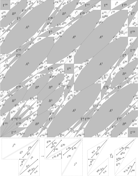
Figure A.1. The first return map $\hat{T}_{3}$ and large parts of $\mathcal{R}$, $\lambda=\sqrt{3}$. ($\ell^{k}$ stands for $T^{k}(D_{\ell})$.)

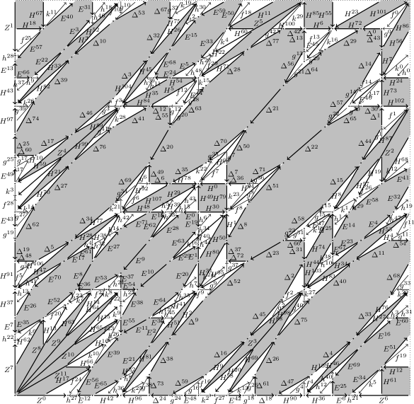
Figure A.2. Trajectories of long lines in $\mathcal{R}$ and $D_{f},D_{g},D_{h},D_{k}$, $\lambda=\sqrt{3}$. ($\ell^{k}$ stands for $T^{k}(D_{\ell})$.)

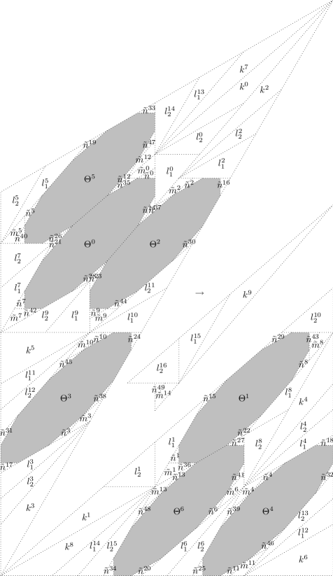
Figure A.3. An intermediate first return map, $\lambda=\sqrt{3}$. ($\ell^{k}$ stands for $\hat{T}_{3}^{k}(D_{\ell})$.)

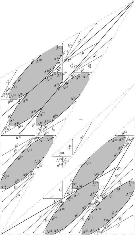
Figure A.4. The trajectory of the lines, $\lambda=\sqrt{3}$. ($\ell^{k}$ stands for $\hat{T}_{3}^{k}(D_{\ell})$.)

Figure A.5. The map $\hat{T}_{4}$, $\lambda=\sqrt{3}$. ($\ell^{k}$ stands for $T^{k}(D_{\ell})$.)

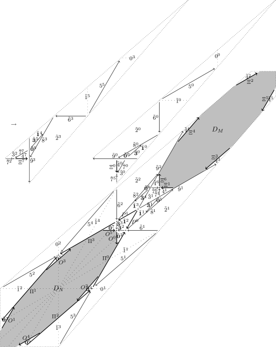
Figure A.6. Almost the map $\hat{T}$, $\lambda=\sqrt{3}$. ($\ell^{k}$ stands for $\hat{T}_{4}^{k}(D_{\ell})$.)

As the scaling domain $\mathcal{D}$ is very small in case $\lambda=\sqrt{3}$, the determination of $\hat{T}$ is done in several steps. Figure A.1 shows the action of $\hat{T}_{3}$, which is the first return map on the domain

$$\{x>4\sqrt{3}-6,2y<\sqrt{3}x+2-\sqrt{3},y>\sqrt{3}x+1-\sqrt{3}\}\cup\{x<1,y>12\sqrt{3}x-20,y>\sqrt{3}x+6\sqrt{3}-11\},$$

on sets $D_{a},\ldots,D_{h}$. To this end, we first determine the trajectory of sets $D_{\tilde{a}},D_{b},\ldots,D_{k}$, which partition a symmetric version of this domain. Figure A.1 shows the trajectory of the open sets $D_{\tilde{a}},D_{b},D_{c},D_{d},D_{e},D_{i},D_{j}$, Figure A.2 completes the picture with the trajectories of the lines $D_{f},D_{g},D_{h},D_{k}$. All points which are not on these trajectories are periodic. ¿From the symmetric first return map, it is easy to determine $\hat{T}_{3}$.

Next, we consider the first return map on

$$\{(x,y):\,2y<\sqrt{3}x+2-\sqrt{3},\,2x<\sqrt{3}y+2-\sqrt{3},\,x\geq 30\sqrt{3}-51\mbox{ or }y\geq 30\sqrt{3}-51\}$$

in Figures A.3 and A.4, partitioned into open sets $D_{k},D_{l_{1}},D_{l_{2}},D_{\tilde{m}},D_{\tilde{n}}$ and lines $D_{l_{3}},D_{o},D_{\tilde{p}},D_{\tilde{q}}$. ¿From this map, we easily obtain the first return map $\hat{T}_{4}$ on $\{(x,y):\,2y<\sqrt{3}x+2-\sqrt{3},\,2x<\sqrt{3}y+2-\sqrt{3},\,x\geq 30\sqrt{3}-51\mbox{ and }y\geq 30\sqrt{3}-51\}$, which is partitioned into the sets $D_{l},\ldots,D_{q}$. Observe that the return time on $D_{l}$ is not constant since the trajectories of the three parts $D_{l_{1}},D_{l_{2}},D_{l_{3}}$ are different. This implies that the return times on $D_{0},D_{1}$ and $D_{\mathbf{0}}$ are not constant.

Finally, we consider in Figure A.6 the first return map on

$$\{(x,y):\,2y<\sqrt{3}x+2-\sqrt{3},\,2x<\sqrt{3}y+2-\sqrt{3},\,x\geq 72-41\sqrt{3}\mbox{ or }y\geq 72-41\sqrt{3}\},$$

partitioned into sets $D_{0},D_{\tilde{1}},\ldots,D_{\tilde{9}},D_{\tilde{\mathbf{0}}},D_{\tilde{\mathbf{1}}},D_{\tilde{\mathbf{3}}}$, from which it is easy to deduce $\hat{T}$ on $\mathcal{D}$.

Appendix B The map $\hat{T}$ for $\lambda=-\sqrt{3}$.

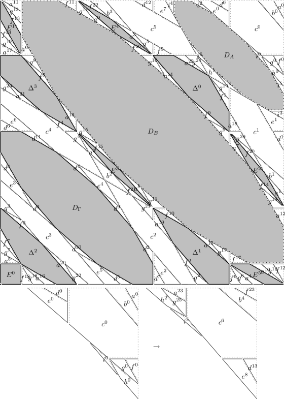
Figure B.1. A first return map and large parts of $\mathcal{R}$, $\lambda=-\sqrt{3}$. ($\ell^{k}$ stands for $T^{k}(D_{\ell})$.)

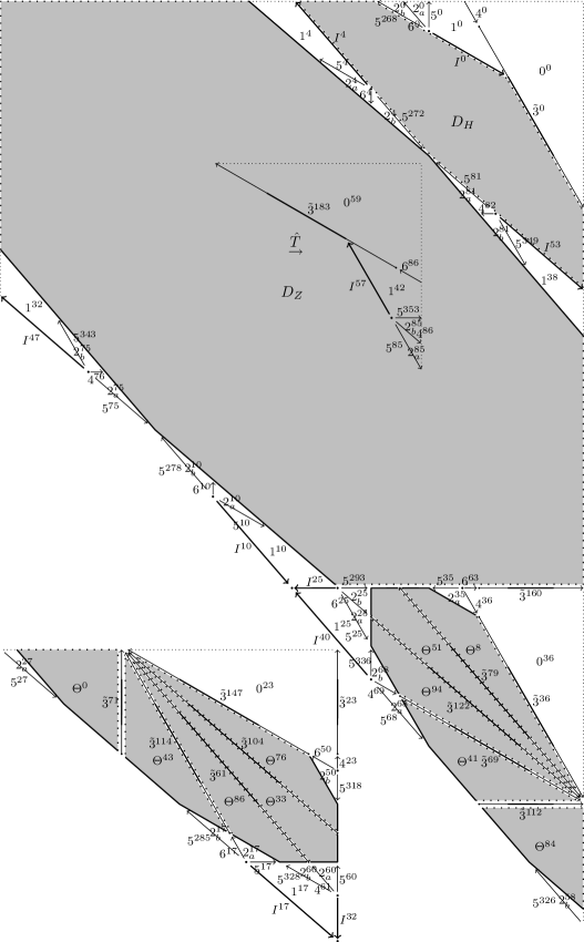
Figure B.2. The map $\hat{T}$ and small parts of $\mathcal{R}$, $\lambda=-\sqrt{3}$. ($\ell^{k}$ stands for $T^{k}(D_{\ell})$.)

For $\lambda=-\sqrt{3}$, we consider in Figure B.1 the first return map on

$$\{(x,y)\in[0,1)^{2}:\,2x+\sqrt{3}y>3\sqrt{3}-2\mbox{ or }\sqrt{3}x+2y>3\sqrt{3}-2\},$$

partitioned into sets $D_{a},\ldots,D_{i}$. Figure B.2 provides the first return map $\hat{T}$ on $\mathcal{D}$. Again, all points in $\mathcal{R}$ are periodic.

References

[1]R.L. Adler, B.P. Kitchens, C.P. Tresser, Dynamics of non-ergodic
piecewise affine maps of the torus, Ergodic Theory Dyn. Syst. 21 (2001),
959–999.
[2]S. Akiyama, T. Borbély, H. Brunotte, A. Pethő,
J. M. Thuswaldner, On a generalization of the radix representation – a
survey, in “High primes and misdemeanours: lectures in honour of the 60th
birthday of Hugh Cowie Williams”, Fields Inst. Commun. 41 (2004), 19–27.
[3]S. Akiyama, H. Brunotte, A. Pethő, W. Steiner, Remarks on a
conjecture on certain integer sequences, Period. Math. Hung. 52 (2006),
1–17.
[4]S. Akiyama, H. Brunotte, A. Pethő, J. Thuswaldner, Generalized
radix representations and dynamical systems II, Acta Arith. 121 (2006),
21–61.
[5]G. Allouche, J.-P. Allouche, J. Shallit, Kolam indiens, dessins sur
le sable aux îles Vanuatu, courbe de Sierpinski et morphismes de
monoïde, Ann. Inst. Fourier 56 (2006), 2115–2130.
[6]J.-P. Allouche, G. Skordev, Von Koch and Thue-Morse revisited,
Fractals 15 (2007), 405–409.
[7]P. Ashwin, Elliptic behaviour in the sawtooth standard map,
Phys. Lett., A 232 (1997), 409–416.
[8]P. Ashwin, W. Chambers, G. Petrov, Lossless digital filters overflow
oscillations: approximations of invariant fractals, Int. J. Bifurcation Chaos
Appl. Sci. Eng. 7 (1997), 2603–2610.
[9]D. Bosio, F. Vivaldi, Round-off errors and adic numbers,
Nonlinearity 13 (2000), 309–322.
[10]L. O. Chua, T. Lin, Chaos in digital filters, IEEE Trans. Circuits
Syst. 35 (1988), 648–658.
[11]A. C. Davies, Nonlinear oscillations and chaos from digital filters
overflow, Phil. Trans. R. Soc. Lond., A 353 (1995), 85–99.
[12]A. Goetz, Dynamics of piecewise isometries, Ill. J. Math. 44
(2000), 465–478.
[13]A. Goetz, Stability of piecewise rotations and affine maps,
Nonlinearity 14 (2001), 205–219.
[14]A. Goetz, Piecewise Isometries — An Emerging Area of Dynamical
Systems, Fractals in Graz 2001, ed. P. Grabner and W. Woess, Birkhäuser,
Basel, 2003, 133–144.
[15]E. Gutkin, N. Haydn, Topological entropy of polygon exchange
transformations and polygonal billiards, Ergodic Theory Dyn. Syst. 17
(1997), 849–867.
[16]E. Gutkin, N. Simanyi, Dual polygonal billiards and necklace
dynamics, Commun. Math. Phys. 143 (1992), 431–449.
[17]B. Khang, Dynamics of symplectic affine maps on tori, PhD Thesis,
University of Illinois at Urbana-Champaign, 2000.
[18]K.L. Kouptsov, J. H. Lowenstein, F. Vivaldi, Quadratic rational
rotations of the torus and dual lattice maps, Nonlinearity 15 (2002),
1795–1842.
[19]J.H. Lowenstein, S. Hatjispyros, F. Vivaldi, Quasi-periodicity,
global stability and scaling in a model of Hamiltonian round-off, Chaos
7 (1997), 49–66.
[20]J. H. Lowenstein, K. L. Kouptsov, F. Vivaldi, Recursive tiling and
geometry of piecewise rotations by , Nonlinearity 17 (2004),
371–395.
[21]J. H. Lowenstein, F. Vivaldi, Anomalous transport in a model of
hamiltonian round-off errors, Nonlinearity 11 (1998), 1321–1350.
[22]J. H. Lowenstein, F. Vivaldi, Embedding dynamics for round-off
errors near a periodic orbit, Chaos 10 (2000), 747–755.
[23]K. Mahler, Some suggestions for further research, Bull. Aust. Math.
Soc. 29 (1984), 101–108.
[26]F. Vivaldi, Periodicity and transport from round-off errors, Exp.
Math. 3 (1994), 303–315.
[27]F. Vivaldi, The arithmetic of discretized rotations, -adic
mathematical physics, AIP Conf. Proc. 826 (2006), Amer. Inst. Phys.,
Melville, NY, 162–173.
[28]F. Vivaldi, J. H. Lowenstein, Arithmetical properties of a family of
irrational piecewise rotations, Nonlinearity 19 (2006), 1069–1097.
[29]F. Vivaldi, A. V. Shaidenko, Global stability of discontinuous dual
billiards, Commun. Math. Phys. 110 (1987), 625–640.
[30]F. Vivaldi, I. Vladimirow, Pseudo-randomness of round-off errors in
discretized linear maps on the plane, Int. J. Bifurcation Chaos Appl. Sci.
Eng. 13 (2003), 3373–3393.
[31]C. W. Wu, L. O. Chua, Properties of admissible sequences in a
second-order digital filter with overflow non-linearity, Int. J. Circuit
Theory Appl. 21 (1993), 299–307.