Different vacua in 2HDM

Abstract

We discuss the extrema of the Two Higgs Doublet Model with different physical properties. We have found necessary and sufficient conditions for realization of the extrema with different properties as the vacuum state of the model. We found explicit equations for extremum energies via parameters of potential if it has explicitly CP conserving form. These equations allow to pick out extremum with lower energy – vacuum state and to look for change of extrema (phase transitions) with the variation of parameters of potential. Our goal is to find general picture here to apply it for description of early Universe.

I Introduction. Motivation

The Two Higgs Doublet Model (2HDM) presents the simplest extension of minimal scheme of Electroweak Symmetry Breaking (EWSB) allowing to include naturally observed CP violation and Flavour Changing Neutral Currents TDLee . Natural approach in its description is to derive its parameters based from modern data and future observations at colliders. This very approach with properties of vacuum, fixed by observations, is developed in many papers(see e.g. hunter -GK05 ). Such approach contains the danger that the discussed set of parameters allow another minimum of potential which is deeper than the discussed one, in this case obtained results correspond not real but false vacuum.

The Models like 2HDM can have different vacuum states (minima of potential) with various physical properties. Another approach appears – to study different vacua in order to confine field of possible values of parameters of Lagrangian allowing description of data (see e.g. GH05 –Barroso2 ).

In this paper we consider different possible vacuum states in 2HDM with two goals.

1). We like to have a complete set of necessary and sufficient conditions for realization of the extrema with different properties as the vacuum state of the model. These conditions must allow to check whether the discussed minimum of potential is global one (vacuum) or not.

2). The obtained results must allow to study (in future works) what can happen at variations of parameters of Lagrangian, related to the evolution of earlier Universe, as it was proposed in Gin06 . Let us describe this idea in more details.

At first moments after Big Bang the temperature of the Universe $T$ was very high, in this stage vacuum expectation values of Higgs fields are given by minimum of the Gibbs potential $V_{G}$. The latter is a sum of the Higgs potential $V(\phi)$ and the term $aT^{2}\phi^{2}$. It corresponds to the Higgs model with parameters varying in time. At large $T$ potential has EW symmetric minimum at $\langle\phi\rangle=0$. This stage describes the widely discussed phenomenon of inflation.

Figure 1: Evolution of Gibbs potential in minimal SM

During the inflatory expansion, the Universe becomes colder, and at some temperature the Gibbs potential transforms effectively into the well known form of the Higgs model with $\langle\phi\rangle\neq 0$ – we obtain our world with massive particles, etc. (EWSB) (see Fig. 1). This phase transition determines the fate of the Universe after inflation.

We see in 2HDM many possible vacuum states depending on interrelation of the parameters of the potential. In the Gibbs potential the temperature dependent addition to the mass term has form $T^{2}a_{ij}(\phi_{i}^{\dagger}\phi_{j})/2$ Gin06 . With these terms the interrelation mentioned above changes during cooling of Universe, this leads to the change of phase state of Universe. The sequence of phase states of Universe during its early history, transitions among vacuum states with different properties can influence for current state of Universe Gin06 .

$\bullet$  For these goals we consider all possible extremum states of the Higgs potential and after that investigate which of these extrema can be the vacuum state – a global minimum of potential. So, in this paper we discuss all types of extremum states in 2HDM and determine conditions when one of them is vacuum state. The obtained explicit form of dependence of different vacuum state energies on parameters of Lagrangian seems to be an important result on this way.

In sect. II we describe the Lagrangian of the model and its general properties. Sect. III is devoted to the description of different extrema of the potential and their first classification. In short sect. IV we discuss conditions when the electroweak symmetry point $\langle\phi_{1}\rangle=\langle\phi_{2}\rangle=0$ can be (local) maximum or minimum of the potential. In the sect. V we study the most exotic type of the extremum – charged extremum, which is not realized in our world – in this extremum the interaction of gauge bosons with fermions will not preserve the electric charge, photon becomes massive, etc. Barroso . However it is not improbable that this state was the vacuum state in some period after Big Bang. Then we come to the general discussion of ”normal” neutral extrema in sect. VI. Their study is continued for the important case of the explicitly CP conserving potential (with all real coefficients) – sect. VII. We discuss in detail uniquely defined doubly generate spontaneously CP violating extrema, sect. VII.1 and CP preserving extrema in sect. VII.2. Then we discuss interrelation among different extrema, sect. VIII. In appendix A we develop a special toy model, for which all the calculations can be done easily. This model gives a simple illustration of many general statements in the main text and provides an answer to problems of realizability of some situations. In sect. IX and X we summarize the results obtained and briefly discuss possible applications for the history of Universe.

II Lagrangian

The spontaneous electroweak symmetry breaking via the Higgs mechanism is described by the Lagrangian

$$\begin{array}[]{c}{\cal L}={\cal L}^{SM}_{gf}+{\cal L}_{H}+{\cal L}_{Y}\;\;with\;\;{\cal L}_{H}=T-V\,,\\[5.69054pt] \phi_{i}=\begin{pmatrix}\phi_{i}^{+}\\ \phi_{i}^{0}\end{pmatrix}.\end{array}$$ (1)

Here ${\cal L}^{SM}_{gf}$ describes the $SU(2)\times U(1)$ Standard Model interaction of gauge bosons and fermions, ${\cal L}_{Y}$ describes the Yukawa interactions of fermions with Higgs scalars and ${\cal L}_{H}$ is the Higgs scalar Lagrangian; $T$ is the Higgs kinetic term and $V$ is the Higgs potential (3). In this paper we won’t consider effects related to possible non-diagonal terms in $T$ (see preliminary discussion in GK05 ).

The Two Higgs Doublet Model is the simplest extension of the minimal SM. It contains two scalar weak isodoublets $\phi_{1}$ and $\phi_{2}$ with identical hypercharge. In particular, it is realized in MSSM. To describe Higgs potential in short form, it is useful to introduce isoscalar combinations of the field operators

$$\begin{array}[]{c}x_{1}=\phi_{1}^{\dagger}\phi_{1},\,\;\;x_{2}=\phi_{2}^{\dagger}\phi_{2},\\[5.69054pt] x_{3}=\phi_{1}^{\dagger}\phi_{2}\,,\;\;x_{3^{*}}\equiv x_{3}^{\dagger}=\phi_{2}^{\dagger}\phi_{1}\,.\end{array}$$ (2)

The most general renormalizable Higgs potential is the sum of the operator $-\;V_{2}$ of dimension 2 and the operator $V_{4}$ of dimension 4:

$$\begin{array}[]{c}V=V_{0}-V_{2}(x_{i})+V_{4}(x_{i})\,;\\ V_{2}(x_{i})=M_{i}x_{i}\equiv\\ \equiv\dfrac{{1}}{{2}}\left[m_{11}^{2}x_{1}\!+\!m_{22}^{2}x_{2}\!+\!\left(m_{12}^{2}x_{3}\!+\!h.c.\right)\right]\,,\\[5.69054pt] V_{4}(x_{i})=\Lambda_{ij}x_{i}x_{j}/2\equiv\\[5.69054pt] \equiv\dfrac{{\lambda_{1}x_{1}^{2}\!+\!\!\lambda_{2}x_{2}^{2}}}{{2}}\!+\!\lambda_{3}x_{1}x_{2}\!+\!\lambda_{4}x_{3}x_{3}^{\dagger}+\\[5.69054pt] +\!\!\left[\dfrac{{\lambda_{5}x_{3}^{2}}}{{2}}\!+\!\lambda_{6}x_{1}x_{3}\!+\!\lambda_{7}x_{2}x_{3}\!+\!h.c.\right]\!.\end{array}$$ (3)

Here $i,\,j=1,\,2,\,3,\,3^{*}$, $\Lambda_{ij}=\Lambda_{ji}$. Besides, $\lambda_{1-4}$ and $m_{ii}^{2}$ are real while $\lambda_{5-7}$ and $m_{12}^{2}$ are generally complex. The field independent term $V_{0}$ is added for convenience in future, we omit this term in many equations below.

$\bullet$  The reparametrization and rephasing symmetry. Our model contains two fields with identical quantum numbers. Therefore, the pure Higgs sector can be described both in terms of fields $\phi_{k}$ $(k=1,2)$, used in Lagrangian (3), and in terms of fields $\phi^{\prime}_{k}$ obtained from $\phi_{k}$ by a generalized rotation. The corresponding reparametrization symmetry was studied in GunionHaber ; GK05 ; Ivan .

In fact, in the description of reality we deal usually with the Yukawa sector, where right hand isosinglet fermion fields of each type are coupled with only one basic field $\phi_{1}$ or $\phi_{2}$ (Model II, like MSSM, or Model I, see hunter ). This property becomes hidden at the general reparametrization transformation. The efficient form of the potential is that in which above property of Yukawa interaction is explicit.

This efficient form of potential retains one degree of freedom – the independent phase transformation of fields $\phi_{i}\to\phi_{i}e^{i\rho_{i}}$ and corresponding phase transformation of parameters of potential are allowed – rephasing (RPh) transformation. RPh symmetry group is the subgroup of reparametrization symmetry group. For Lagrangian it is one-parametric group with single parameter$\rho_{1}-\rho_{2}$. Below we have in mind mentioned efficient form of potential and RPh freedom for it.

The potential with explicit CP conservation is that with all real $\lambda_{i}$, $m^{2}_{12}$ (or with parameters which can be transformed to real ones by single RPh transformation).

$\bullet$  The results for the most general Lagrangian (presented below) often have very complex form. Main features of physical picture are seen in more simple potential with softly broken $Z_{2}$ symmetry , in which $\lambda_{6}=\lambda_{7}=0$. We will discuss many results using final equations for this very potential, often – in the explicit CP conserving case.

$\bullet$  Positivity constraints. To have a stable vacuum, the potential must be positive at large quasi–classical values of fields $|\phi_{k}|$ (positivity constraints) for an arbitrary direction in the $(\phi_{1},\phi_{2})$ plane. It means that upon replacement of the operators $x_{i}$ with some numbers $z_{i}$

$$V_{4}(z_{i})>0\;\;\;\;if\;\;\;\;z_{1}\,,\;z_{2}>0\,,\;\;\;z_{1}z_{2}-z_{3}z_{3}^{*}\geq 0\,.$$ (4a)

This condition limits possible values of $$\lambda_{i} Z_{2} \lambda_{6}=\lambda_{7}=0$$. For the potential with softly broken symmetry () such limitations have form (see e.g. dema ; GIv )

$$\begin{array}[]{c}\lambda_{1}>0\,,\quad\lambda_{2}>0,\;\,\sqrt{\lambda_{1}\lambda_{2}}+\lambda_{3}>0,\\[5.69054pt] \sqrt{\lambda_{1}\lambda_{2}}+\lambda_{3}+\lambda_{4}-|\lambda_{5}|>0\,.\par\end{array}$$ (4b)

III Extrema of potential

The extrema of the potential define the values $\langle\phi_{1,2}\rangle$ of the fields $\phi_{1,2}$ via equations:

$$\partial V/\partial\phi_{i}|_{\phi_{i}=\langle\phi_{i}\rangle}=0\,,\qquad\partial V/\partial\phi_{i}^{\dagger}|_{\phi_{i}=\langle\phi_{i}\rangle}=0\,.$$ (5)

These equations have the electroweak symmetry conserving (EWc) solution $\langle\phi_{i}\rangle=0$ and the electroweak symmetry breaking (EWSB) solutions. Here and below notation $\langle F\rangle$ mean numerical value of the operator $F$ at extremum. In general, there are many EWSB extrema. We label these extrema by an additional subscript, if necessary; e.g. $\langle F\rangle_{N}$ means value of $\langle F\rangle$ in $N$-th extremum.

We consider also the values $y_{i}$ of operators $x_{i}$ at the extremum points. In the discussed tree approximation (mean field in the statistical physics) we have

$$y_{i,N}\equiv\langle x_{i}\rangle_{N}=\langle\phi_{a}\rangle_{N}^{\dagger}\,\langle\phi_{b}\rangle_{N}\qquad\mbox{for}\qquad x_{i}=\phi_{a}^{\dagger}\phi_{b}\,.$$

In each extremum point these values obey inequalities following from definition and Cauchy inequality, written for important auxiliary quantity $Z$:

$$y_{1}>0\,,\quad y_{2}>0\,,\qquad Z=y_{1}y_{2}-y_{3}^{*}y_{3}\geq 0\,.$$ (6)

$\bullet$  Classification of EWSB extrema. It is useful to define quantities

$$\begin{array}[]{c}T_{a}\equiv\langle\partial V/\partial x_{a}\rangle=\Lambda_{ai}y_{i}-M_{a}\,\quad(a=1,\,2,\,3,\,3^{*})\,,\\[5.69054pt] T_{1,2}\quad are\;\;real,\qquad T_{3^{*}}=T_{3}^{*}\,.\end{array}$$ (7)

In these terms eq. (5) have form

$$\begin{array}[]{lc}\langle\partial V/\partial\phi_{1}^{\dagger}\rangle=&\langle\phi_{1}\rangle T_{1}+\langle\phi_{2}\rangle T_{3}=0\,,\\[5.69054pt] \langle\partial V/\partial\phi_{2}^{\dagger}\rangle=&\langle\phi_{2}\rangle T_{2}+\langle\phi_{1}\rangle T_{3^{*}}=0\,,\\[5.69054pt] \langle\partial V/\partial\phi_{1}\rangle=&\langle\phi_{1}\rangle^{\dagger}T_{1}+\langle\phi_{2}\rangle^{\dagger}T_{3^{*}}=0\,,\\[5.69054pt] \langle\partial V/\partial\phi_{2}\rangle=&\langle\phi_{2}\rangle^{\dagger}T_{2}+\langle\phi_{1}\rangle^{\dagger}T_{3}=0\,.\end{array}$$ (8)

These equations can be easily transformed to equations for $y_{i}$. For example,

$$\begin{array}[]{c}\langle\phi_{1}\rangle^{\dagger}\langle\partial V/\partial\phi_{1}^{\dagger}\rangle=y_{1}T_{1}+y_{3}T_{3}=0\,,\\[5.69054pt] \langle\phi_{2}\rangle^{\dagger}\langle\partial V/\partial\phi_{1}^{\dagger}\rangle=y_{3}^{*}T_{1}+y_{2}T_{3}=0\,,\\[5.69054pt] \langle\phi_{2}\rangle^{\dagger}\langle\partial V/\partial\phi_{2}^{\dagger}\rangle=y_{2}T_{2}+y_{3}^{*}T_{3^{*}}=0\,,\\[5.69054pt] \langle\phi_{1}\rangle^{\dagger}\langle\partial V/\partial\phi_{2}^{\dagger}\rangle=y_{3}T_{2}+y_{1}T_{3^{*}}=0\,.\end{array}$$

One can consider each pair of these equations as a system for calculation of quantities $T_{i}$ via $y_{i}$. The determinant of these systems are precisely $Z=y_{1}y_{2}-y_{3}^{*}y_{3}$. Therefore, it is natural to distinguish two types of extrema, with $Z\neq 0$ (”charged extrema” with $T_{i}=0$) and with $Z=0$ (”neutral extrema” with $T_{i}\neq 0$).

$\bullet$   For each EWSB extremum one can choose the $z$ axis in the weak isospin space so that $\langle\phi_{1}\rangle=\begin{pmatrix}0\\ v_{1}\end{pmatrix}$ with real $v_{1}>0$ (choose ”neutral direction”). In such basis $\langle\phi_{2}\rangle$ has generally an arbitrary form. Then, after this choice the most general electroweak symmetry violating solution of (5) can be written in a form with real $v_{1}$ and complex $v_{2}$:

$$\begin{array}[]{c}\langle\phi_{1}\rangle=\dfrac{{1}}{{\sqrt{2}}}\left(\begin{array}[]{c}0\\ v_{1}\end{array}\right),\quad\langle\phi_{2}\rangle=\dfrac{{1}}{{\sqrt{2}}}\left(\begin{array}[]{c}u\\ v_{2}\end{array}\right)\\[11.38109pt] with\;\;v_{1}=|v_{1}|,\;v_{2}=|v_{2}|e^{i\xi}\,,\end{array}$$ (9)

without loss of generality we can consider only real positive $u$.

At $u\neq 0$ we have $Z>0$ – charged extremum, at $u=0$ we have $Z=0$ – neutral extremum.

$\bullet$  Mass matrix at each extremum is given by the decomposition of the fields $\phi_{i}$ near the extremum point. Since the position of an extremum point relative to origin of coordinates selects some direction in the isospace, this matrix has different elements for different components of fields

$$M_{ij,\alpha\beta}=\dfrac{{\partial^{2}V}}{{\partial\phi_{i}^{\beta}\partial\phi_{j}^{*\alpha}}}\,,(i,\,j\,=1,\,2\,,\;\;\alpha\,,\beta=+,\,0)\,.$$ (10a)

Direct differentiation gives

$$\begin{array}[]{c}M_{11,\alpha\beta}=T_{1}\delta_{\alpha\beta}+\Lambda_{11}\langle\phi_{1\beta}\rangle^{\dagger}\langle\phi_{1}\rangle_{\alpha}+\\ \!\!\!+\Lambda_{13}^{*}\langle\phi_{2\beta}\rangle^{\dagger}\langle\phi_{1\alpha}\rangle+\!\Lambda_{31}\langle\phi_{1\beta}\rangle^{\dagger}\langle\phi_{2\alpha}\rangle+\\ +\!\Lambda_{33^{*}}\langle\phi_{2\beta}\rangle^{\dagger}\langle\phi_{2\alpha}\rangle\,,\\[5.69054pt] M_{12,\alpha\beta}=T_{3}\delta_{\alpha\beta}+\Lambda_{12}\langle\phi_{2\beta}\rangle^{\dagger}\langle\phi_{1\alpha}\rangle+\\ \!\!\!+\Lambda_{13^{*}}\langle\phi_{1\beta}\rangle^{\dagger}\langle\phi_{1\alpha}\rangle+\!\Lambda_{32}\langle\phi_{2\beta}\rangle^{\dagger}\langle\phi_{2\alpha}\rangle+\\ +\!\Lambda_{33^{*}}\langle\phi_{1\beta}\rangle^{\dagger}\langle\phi_{2\alpha}\rangle\,,\\[5.69054pt] M_{21,\alpha\beta}=T_{3^{*}}\delta_{\alpha\beta}+\Lambda_{12}\langle\phi_{2\beta}\rangle\langle\phi_{1\alpha}\rangle^{\dagger}+\\ \!\!\!+\Lambda_{13^{*}}\langle\phi_{1\beta}\rangle\langle\phi_{1\alpha}\rangle^{\dagger}+\!\Lambda_{3^{*}2}\langle\phi_{2\beta}\rangle\langle\phi_{2\alpha}\rangle^{\dagger}+\\ +\!\Lambda_{33^{*}}\langle\phi_{1\beta}\rangle\langle\phi_{2\alpha}\rangle^{\dagger}\,,\\[5.69054pt] M_{22,\alpha\beta}=T_{2}\delta_{\alpha\beta}+\Lambda_{22}\langle\phi_{2\beta}\rangle^{\dagger}\langle\phi_{2\alpha}\rangle+\\ \!\!\!+\Lambda_{23}\langle\phi_{1\beta}\rangle^{\dagger}\langle\phi_{2\alpha}\rangle+\!\Lambda_{3^{*}2}\langle\phi_{2\beta}\rangle^{\dagger}\langle\phi_{1\alpha}\rangle+\\ +\!\Lambda_{33^{*}}\langle\phi_{1\beta}\rangle^{\dagger}\langle\phi_{1\alpha}\rangle\,.\end{array}$$ (10b)

$\bullet$   The distances from some extremum and between two extrema are defined as

$$\begin{array}[]{c}{\cal D}(\phi,N)=\\ \!\!=\!\left(\phi_{1}\langle\phi_{2}\rangle_{N}\!-\!\phi_{2}\langle\phi_{1}\rangle_{N}\right)^{\dagger}\left(\phi_{1}\langle\phi_{2}\rangle_{N}\!-\!\phi_{2}\langle\phi_{1}\rangle_{N}\rangle\right)\!\equiv\!\\[5.69054pt] \equiv x_{1}y_{2}+x_{2}y_{1}-x_{3}y_{3^{*}}-x_{3}^{\dagger}y_{3}\,,\\[5.69054pt] {\cal D}(I,II)\!\equiv\!\langle{\cal D}(\phi,II)\rangle_{I}\!\equiv\!\langle{\cal D}(\phi,I)\rangle_{II}\!\equiv\!{\cal D}(II,I)\!=\!\\[5.69054pt] =|\left(\langle\phi_{1,I}\rangle\langle\phi_{2,II}\rangle-\langle\phi_{2,I}\rangle\langle\phi_{1,II}\rangle\right)|^{2}\,.\end{array}$$ (11)

Note that ${\cal D}(\phi,N)=0$ at $\phi_{i}=\langle\phi_{i}\rangle_{N}$ and ${\cal D}(I,II)>0$ for a pair of different extrema.

$\bullet$  The extremum energy is

$$\begin{array}[]{c}{\cal E}_{N}^{ext}=V(\langle\phi_{i}\rangle_{N})\equiv\\[5.69054pt] \equiv V(y_{i,N})=V_{0}-V_{2}(y_{i,N})+V_{4}(y_{i,N})\,.\end{array}$$ (12)

According to theorem on homogeneous functions, in each extremum point

$$\begin{array}[]{c}\Lambda_{ij}y_{i,N}y_{j,N}=M_{i}y_{i,N}\,,\quad or\;\;equivalently\\[5.69054pt] \;\;V_{2}(\langle\phi_{i}\rangle_{N})=2V_{4}(\langle\phi_{i}\rangle_{N})\,\Rightarrow\\[5.69054pt] \Rightarrow{\cal E}_{N}^{ext}=V_{0}-V_{4}(y_{i,N})=V_{0}-V_{2}(y_{i,N})/2\,.\end{array}$$ (13)

The extremum with the lowest value of energy (the global minimum of potential) realizes the vacuum state of the model. Other extrema can be either saddle points or maxima or local minima of the potential. It can be established, in particular, by the study of the effective mass matrix at these extrema.

$\bullet$  Decomposition around EWSB extremum. Our potential can be rewritten as a sum of extremum energy and terms vanishing in the extremum point together with their derivatives in $\phi_{i}$. This polynomial with terms up to the second order in $x_{i}$ can be written as a sum of polynomials of second and first orders in $x_{i}$ vanishing together with their derivatives in the extremum point. The form of second order polynomial is fixed by a quartic terms of potential, it can be only $V_{4}(x_{i}-y_{i})$. The residuary first order polynomial in $x_{i}$ must be proportional to ${\cal D}(\phi,N)$. Therefore

$$V={\cal E}_{N}^{ext}+V_{4}(x_{i}-y_{i,N})+{\cal R}\cdot{\cal D}(\phi,N)\,.$$ (14a)

It means that the mass terms of (3) can be written via quantities $$y_{i}$$ in a following way

$$\begin{array}[]{c}m_{11}^{2}=2\left(\lambda_{1}y_{1}+\lambda_{3}y_{2}+\lambda_{6}y_{3}+\lambda_{6}^{*}y_{3^{*}}-y_{2}{\cal R}\right)\,,\\ m_{22}^{2}=2\left(\lambda_{3}y_{1}+\lambda_{2}y_{2}+\lambda_{7}y_{3}+\lambda_{7}^{*}y_{3^{*}}-y_{1}{\cal R}\right)\,,\\ m_{12}^{2}=2\left(\lambda_{6}y_{1}+\lambda_{7}y_{2}+\lambda_{5}y_{3}+\lambda_{4}y_{3^{*}}-y_{3^{*}}{\cal R}\right)\,.\\ \end{array}$$ (14b)

The differentiation of (14a) gives for $$T_{i}$$:

$$T_{1}=y_{2}{\cal R}\,,\quad T_{2}=y_{1}{\cal R}\,,\quad T_{3}=-y_{3}^{*}{\cal R}\,,\quad T_{3^{*}}=-y_{3}{\cal R}\,.$$

In accordance with (8) for charged extremum we have from here ${\cal R}=0$.

For the neutral extremum the Higgs fields mass matrix (10b) for the upper ($\pm$) components can be written as

$$M_{++}=\begin{pmatrix}T_{1}&T_{3}\\ T_{3^{*}}&T_{2}\end{pmatrix}\equiv\begin{pmatrix}y_{2}&-y_{3}^{*}\\ -y_{3}&y_{1}\end{pmatrix}{\cal R}\,.$$

At $Z=0$ determinant of this matrix equals to 0. Therefore, one  eigenstate of this matrix equals to 0. It describes massless combination of charged Higgs fields (well known Goldstone state). The second eigenstate of above matrix describes the physical charged Higgs boson with mass

$$M_{H^{\pm}}^{2}=Tr\;M_{++}=T_{1}+T_{2}=(y_{1}+y_{2}){\cal R}\,.$$

This quantity is positive for the minimum of the potential, it can be negative in other extremes. Finally, we obtain

$$\begin{array}[]{c l}{\cal R}=0&\;\;\mbox{\it for charged extremum}\\[2.84526pt] \left.{\cal R}=\dfrac{{M_{H^{\pm}}^{2}}}{{y_{1}+y_{2}}}\right|_{N}&\;\;\mbox{\it for neutral extremum}\;N\,.\end{array}$$ (14c)

IV EW symmetry conserving (EWc) point

The EWc point $\langle\phi_{1}\rangle=\langle\phi_{2}\rangle=0$ is extremum of potential. Depending on $m_{ij}^{2}$ it has different nature:

$$\begin{array}[]{crc}At&\begin{array}[]{c}m_{11}^{2}<0\,,\;m_{22}^{2}<0\,,\\[5.69054pt] m_{11}^{2}>0\,,\;m_{22}^{2}>0\end{array}\;\;and\;\;m_{11}^{2}m_{22}^{2}\geq|m_{12}^{2}|^{2}&\begin{array}[]{c}\vspace{-2mm}-\;\mbox{\it minimum}\,,\\[5.69054pt] -\;\mbox{\it maximum}\,,\end{array}\\[8.53581pt] At&\;\;m_{11}^{2}m_{22}^{2}<|m_{12}^{2}|^{2}&-\,saddle\;\;point.\end{array}$$ (15)

According to Ivan no other extremum can be a maximum of potential.

V Charged extremum

We consider now the extremum which appears at

$$Z=y_{1}y_{2}-y_{3}^{*}y_{3}\neq 0\;\;\Rightarrow\;\;u\neq 0\,.$$ (16)

If this extremum realizes the vacuum, it is not possible to split the gauge boson mass matrix into the neutral and charged sectors, the interaction of gauge bosons with fermions will not preserve electric charge, photon becomes massive, etc. Barroso . That is the reason why this extremum is called the charged extremum. We label quantities related to this extremum by a subscript $N=ch$, if necessary.

Certainly, this case is not realized in our World. Nevertheless, it is interesting to consider main features of the case when this extremum is the vacuum state in respect to the opportunity of different scenarios in the Early Universe.

In the considered case eqs. (8) for the extremum of the potential have form

$$\begin{array}[]{c}T_{1}=\lambda_{1}y_{1}\!+\!\lambda_{3}y_{2}\!+\!\lambda_{6}^{*}y_{3}^{*}+\lambda_{6}y_{3}-m_{11}^{2}/2=0,\\[2.84526pt] T_{2}=\lambda_{2}y_{2}\!+\!\lambda_{3}y_{1}\!+\!\lambda_{7}^{*}y_{3}^{*}+\lambda_{7}y_{3}-m_{22}^{2}/2=0,\\[2.84526pt] T_{3}=\lambda_{4}y_{3}^{*}\!+\!\lambda_{5}y_{3}\!+\!\lambda_{6}y_{1}+\lambda_{7}y_{2}-m_{12}^{2}/2=0,\\ T_{3^{*}}=\lambda_{4}y_{3}\!+\!\lambda_{5}^{*}y_{3}^{*}\!+\!\lambda_{6}^{*}y_{1}+\lambda_{7}^{*}y_{2}-m_{12}^{*2}/2=0.\end{array}$$ (17)

That is a system of linear equations for $y_{i}$. It can have only one unique solution (except some degenerate cases) –  system can have only one charged extremum.

This system has solution at arbitrary parameters of the potential. However, in accordance with (9), it describes an extremum of the original potential (3) (we define some quantities $v_{i}$ and $u$) if only the obtained values $y_{1,2}$ obey inequalities $y_{1}>0$, $y_{2}>0$, $Z>0$ (6). In this case

$$\begin{array}[]{c}v_{1}=\sqrt{2y_{1}}\,,\;\;|v_{2}|=\sqrt{2y_{3}y^{*}_{3}/y_{1}}\,,\\[5.69054pt] u=\sqrt{2Z/y_{1}}\,,\;\;e^{2i\xi}=y_{3}/y_{3}^{*}\,.\end{array}$$ (18)

Inequalities (6) determine the range of possible values of $\lambda_{i}$ and $m_{ij}^{2}$ where the charged extremum can exist.

$\bullet$  Condition for minimum. In the discussed case the potential (3) can be rewritten in the form (14) with ${\cal R}=0$. The charged extremum is minimum of the potential if the quadratic form $V_{4}(x_{i}-y_{i,ch})$ is positively defined at each classical value of operators $x_{i}$. This condition differs from the positivity constraint (4a), since quantities $z_{i}=x_{i}-y_{i,ch}$ do not need to satisfy conditions given in this constraint. Here $z_{1}$ and $z_{2}$ are some real quantities (positive or negative) and $z_{3}=z_{3^{*}}^{*}$ is an independent complex quantity. Therefore, the condition for the charged minimum is (see e.g. Ivan )

$$V_{4}(z_{i})\geq 0\;at\;arbitrary\;real\;z_{1},\,z_{2},\;comp\,lex\;\;z_{3}\,.$$ (19)

$\bullet$  The case of softly broken $Z_{2}$ symmetry($\lambda_{6}=\lambda_{7}=0$). The main features of the solution are seen in the case of the soft $Z_{2}$ symmetry violation. In this case solution of equation (17) has form

$$\begin{array}[]{c}y_{1}=\dfrac{{m_{11}^{2}\lambda_{2}\!-\!m_{22}^{2}\lambda_{3}}}{{2(\lambda_{1}\lambda_{2}-\lambda_{3}^{2})}}\,,\;\;y_{2}=\dfrac{{-m_{11}^{2}\lambda_{3}\!+\!m_{22}^{2}\lambda_{1}}}{{2(\lambda_{1}\lambda_{2}-\lambda_{3}^{2})}}\,,\\[11.38109pt] y_{3}=\dfrac{{-m_{12}^{2}\lambda_{5}^{*}\!+\!m_{12}^{*2}\lambda_{4}}}{{2(\lambda_{4}^{2}-\lambda_{5}\lambda_{5}^{*})}}.\end{array}$$ (20)

Conditions (6) limit the domain in the space of parameters, where the charged extremum can exist.

The first condition in (6) reads as

$$\begin{array}[]{c}\dfrac{{(m_{11}^{2}\lambda_{2}-m_{22}^{2}\lambda_{3})(m_{22}^{2}\lambda_{1}-m_{11}^{2}\lambda_{3})}}{{(\lambda_{1}\lambda_{2}-\lambda_{3}^{2})^{2}}}\,-\\[5.69054pt] \quad-\left|\dfrac{{m_{12}^{{\dagger}2}\lambda_{4}-m_{12}^{2}\lambda_{5}^{{\dagger}}}}{{\lambda_{4}^{2}-\lambda_{5}\lambda_{5}^{{\dagger}}}}\right|^{2}>0\,.\end{array}$$ (21a)

The specific form of condition $y_{1,2}>0$ depends on the value of parameter $\lambda_{3}$ admissible by the positivity constraint (4b):

$$\begin{array}[]{c}\begin{array}[]{c}m_{11}^{2}\lambda_{2}\!>\!m_{22}^{2}\lambda_{3},\\[8.53581pt] m_{22}^{2}\lambda_{1}\!>\!m_{11}^{2}\lambda_{3}\end{array}\;at\;\;\dfrac{{|\lambda_{3}|}}{{\sqrt{\lambda_{1}\lambda_{2}}}}<1\,;\\[17.07164pt] \begin{array}[]{c}m_{11}^{2}\lambda_{2}\!<\!m_{22}^{2}\lambda_{3},\\[8.53581pt] m_{22}^{2}\lambda_{1}\!<\!m_{11}^{2}\lambda_{3}\end{array}\;at\;\;\dfrac{{\lambda_{3}}}{{\sqrt{\lambda_{1}\lambda_{2}}}}>1\,.\end{array}$$ (21b)

If $\lambda_{5}$ and $m_{12}^{2}$ are real (explicitly CP conserved potential), condition (21a) forbids also small values of $\lambda_{4}+\lambda_{5}$.

The extremum energy in this case is subdivided into the sum of $Z_{2}$ symmetry conserving term and $Z_{2}$ symmetry violating term:

$$\begin{array}[]{c}{\cal E}_{ch}^{ext}\!=\!-\dfrac{{m_{11}^{4}\lambda_{2}\!+\!m_{22}^{4}\lambda_{1}\!-\!2m_{11}^{2}m_{22}^{2}\lambda_{3}}}{{8(\lambda_{1}\lambda_{2}-\lambda_{3}^{2})}}\,-\\[8.53581pt] -\dfrac{{2m_{12}^{{\dagger}2}m_{12}^{2}\lambda_{4}-m_{12}^{{\dagger}4}\lambda_{5}-m_{12}^{4}\lambda_{5}^{\dagger}}}{{8(\lambda_{4}^{2}-\lambda_{5}\lambda_{5}^{{\dagger}})}}\,.\end{array}$$ (22)

This extremum is the minimum of the potential (charged minimum) if condition (19) is satisfied. In the considered case it is easy to obtain (with argumentation similar to that in GIv ) that this condition is satisfied if

$$\lambda_{1}>0\,,\;\;\lambda_{2}>0\,,\;\;\sqrt{\lambda_{1}\lambda_{2}}+\lambda_{3}>0,\;\;\lambda_{4}>|\lambda_{5}|\,.$$

Note that latter condition guarantees negativity of second item in (22).

VI Neutral extrema, general case

Other solutions of the extremum condition (5) obey a condition for $U(1)$ symmetry of electromagnetism, that is solution with

$$\begin{array}[]{c}\boxed{Z=y_{1}y_{2}-y_{3}^{*}y_{3}=0}\Rightarrow\\[5.69054pt] \Rightarrow\langle\phi_{1}\rangle\!=\!\dfrac{1}{\sqrt{2}}\begin{pmatrix}0\\ v_{1}\end{pmatrix},\,\,\langle\phi_{2}\rangle\!=\!\dfrac{1}{\sqrt{2}}\begin{pmatrix}0\\ v_{2}=|v_{2}|e^{i\xi}\end{pmatrix}\,,\\[14.22636pt] \mbox{\it another parameterization:}\\[5.69054pt] v_{1}=v\,cos\beta\,,\quad v_{2}=v\,sin\beta\,,\\[5.69054pt] v^{2}=2(y_{1}+y_{2})=2\left(|\langle\phi_{1}\rangle|^{2}+|\langle\phi_{2}\rangle|^{2}\right)>0\,,\\[5.69054pt] e^{2i\xi}=y_{3}/y_{3}^{*}\,.\end{array}$$ (23)

In this case quantities $y_{i}$ are not independent. Therefore, the field values at the extremum point cannot be obtained by minimization of form (12) in $y_{i}$. In these terms system of equations for v.e.v.’s has form (8) with solutions $y_{i}=y_{i,n}$. It is important to note that the number of independent parameters here is 3 (not 4). Those are the real quantities $y_{1}$, $y_{2}$ and the phase difference of values of fields at the extremum point $\xi$ (not separate phases of these values!).

$\bullet$  Charged Higgs mass. It is useful to reproduce here the equation for the charged Higgs mass, given e.g. in GK05 (eq. (4.3)).

$$\begin{array}[]{c}M_{H^{\pm}}^{2}=v^{2}\left\{\dfrac{{Re\left(\left[m_{12}^{2}\!-\!2(\lambda_{6}y_{1}\!+\!\lambda_{7}y_{2})\right]e^{-i\xi}\right)}}{{4\sqrt{y_{1}y_{2}}}}-\right.\\[5.69054pt] \left.-\dfrac{{\lambda_{4}+Re(\lambda_{5}e^{-2i\xi})}}{{2}}\right\}\,.\end{array}$$ (24a)

In addition, we present corrected eq. (4.5c) from GK05 which gives mass of either pseudoscalar Higgs in the case of CP conservation or intermediate quantity obtained at partial diagonalization of mass matrix in the case of CP violation

$$M_{33}\equiv M_{A}^{2}=M_{H^{\pm}}^{2}+\dfrac{{v^{2}}}{{2}}\left(\lambda_{4}-Re(\lambda_{5}e^{-2i\xi})\right)\,.$$ (24b)

$\bullet$  For the Higgs potential of general form we have no idea about classification of neutral extrema. However, if CP conserving extremum (with no scalar-pseudoscalar mixing) exists, there is a basis in $(\phi_{1},\,\phi_{2})$ space in which potential has explicitly CP conserving form GH05 , GK05 (with all real $\lambda_{i}$, $m^{2}_{ij}$). Using such a form of potential, the subsequent useful classification can be introduced, in this important case.

VII Neutral extrema, case of explicit CP conservation (real $\lambda_{i}$, $m^{2}_{ij}$)

In accordance with definitions (9), we have for each solution $y_{3}=\sqrt{y_{1}y_{2}}\,e^{i\xi}$. In the discussed case the extremum energy (12) is transformed to the form

$$\begin{array}[]{c}{\cal E}^{ext}=-\dfrac{{1}}{{2}}\left\{m_{11}^{2}y_{1}\!+\!m_{22}^{2}y_{2}\!+\!2m_{12}^{2}\sqrt{y_{1}y_{2}}cos\xi\right\}\!+\\[5.69054pt] +\dfrac{\lambda_{1}}{2}y_{1}^{2}+\dfrac{\lambda_{2}}{2}y_{2}^{2}+(\lambda_{3}+\lambda_{4})y_{1}y_{2}+\\[5.69054pt] +\lambda_{5}y_{1}y_{2}cos2\xi+2\left(\lambda_{6}y_{1}+\lambda_{7}y_{2}\right)\sqrt{y_{1}y_{2}}cos\xi.\end{array}$$ (25)

Now we find extrema in coordinates $y_{1}$, $y_{2}$, $\xi$. We start from the minimization in $\xi$ at fixed $y_{i}$. It gives two types of solutions:

$$\begin{array}[]{c}[A]:\;\;\cos\xi=\dfrac{{m_{12}^{2}-2(\lambda_{6}y_{1}+\lambda_{7}y_{2})}}{{4\lambda_{5}\sqrt{y_{1}y_{2}}}}\,,\\[11.38109pt] [B]:\;\;\sin\xi=0\,.\end{array}$$ (26)

For the discussed explicitly CP conserving potential this equation is equivalent to the constraint eq. (3.11) obtained in GK05 .

VII.1 Spontaneously CP violating extremum

The extremum point (26[A]) describes a solution with complex value of field $v_{2}$ at real parameters of the potential. The rephasing transformation $\phi_{2}\to\phi_{2}e^{-i\xi}$ transforms the potential to the real vacuum form, in which parameters of the potential become complex, giving CP violation in the Higgs sector (mixing of scalar and pseudoscalar neutral Higgs bosons) – see for details e.g. GK05 . That is the reason why this extremum is called the spontaneously CP violating (sCPv) extremum TDLee ; Barroso .

The substitution of $cos\xi$ (26) into (25) results in

$$\begin{array}[]{c}E_{sCPv}=\dfrac{\lambda_{1}y_{1}^{2}+\lambda_{2}y_{2}^{2}}{2}+\widetilde{\lambda}_{345}y_{1}y_{2}\,\,-\\[5.69054pt] -\dfrac{{m_{11}^{2}y_{1}+m_{22}^{2}y_{2}}}{{2}}-\dfrac{{[m_{12}^{2}-2(\lambda_{6}y_{1}+\lambda_{7}y_{2})]^{2}}}{{8\lambda_{5}}}\\[8.53581pt] (here\;\;\widetilde{\lambda}_{345}=\lambda_{3}+\lambda_{4}-\lambda_{5})\,.\end{array}$$ (27)

Further minimization gives the system of linear equations $\partial E_{sCPv}/\partial y_{1}=0$, $\partial E_{sCPv}/\partial y_{2}=0$ (we don’t present this general system only due to its bulkiness). Only one solution of this system exists, so y_1,y_2$and$cosξ$aredescribedbyparametersofthepotentialunambiguously$. (This conclusion can be obtained also from the description of Ivan .)

The discussed extremum can be realized only in the range of parameters of the potential obeying inequalities

$$\begin{array}[]{c}\left|\dfrac{{m_{12}^{2}-2(\lambda_{6}y_{1}+\lambda_{7}y_{2})}}{{4\lambda_{5}\sqrt{y_{1}y_{2}}}}\right|=|\cos\xi|<1\,,\\[11.38109pt] y_{1}>0\,,\;\;y_{2}>0\,.\end{array}$$ (28)

The change $\langle\phi_{2}\rangle\to\langle\phi_{2}\rangle^{*}$ ($\xi\to-\;\xi$) does not modify the extremum energy (25). Therefore

if $$\phi_{1}=\langle\phi_{1}\rangle \phi_{2}=\langle\phi_{2}\rangle \Rightarrow\;\phi_{1}=\langle\phi_{1}\rangle \phi_{2}=\langle\phi_{2}\rangle^{*}$$, is the extremum of potential , is also the extremum; these two extrema are degenerate in energy TDLee and define two ”directions” of CP violation, ”left” and ”right”, with (29)

$$\xi=\pm\arccos\left(\dfrac{{m_{12}^{2}-2(\lambda_{6}y_{1}+\lambda_{7}y_{2})}}{{4\lambda_{5}\sqrt{y_{1}y_{2}}}}\right)\,.$$ (30)

$\bullet$  Our potential (25) is a second order polynomial in $\cos\xi$. The sCPv extremum (if it exist) can be a minimum only if $\lambda_{5}>0$, in accordance with GunionHaber .

$\bullet$  Substituting the $\cos\xi$ (26) into (24a) we obtain alternative form for the mass of $H^{\pm}$ and $M_{33}$ in sCPv extremum

$$\begin{array}[]{c}M_{H^{\pm},sCPv}^{2}=\dfrac{{v^{2}}}{{2}}(\lambda_{5}-\lambda_{4})\,,\\[5.69054pt] M_{33,sCPv}=v^{2}\lambda_{5}\sin^{2}\xi\,.\end{array}$$ (31)

To realize minimum of potential, all mass squared eigenvalues and all diagonal terms of squared mass matrix must be positive. Therefore, necessary conditions for realization of sCPv minimum are

$$\lambda_{5}>0\,,\qquad\lambda_{5}>\lambda_{4}\,.$$ (32)

Note that the mass matrix for neutral Higgses in this scPv extremum can be written as (sign $\cdot\cdot\cdot$ mean the diagonal symmetric quantity from the upper right corner of matrix)

$${\cal M}=\begin{pmatrix}M_{11}&M_{12}&v^{2}(\lambda_{5}s_{\beta}\cos\xi+\lambda_{6}c_{\beta})\sin\xi\\ \cdot\cdot\cdot&M_{22}&v^{2}(\lambda_{5}c_{\beta}\cos\xi+\lambda_{7}s_{\beta})\sin\xi\\ \cdot\cdot\cdot&\cdot\cdot\cdot&\lambda_{5}\sin^{2}\xi\end{pmatrix}\,.$$

It shows that – as it is naturally expected – the CP-violating field mixing is weak if the phase $\xi$ is small. Moreover, in the case of soft $Z_{2}$ symmetry violation($\lambda_{6}=\lambda_{7}=0$) physical CP violation is absent at $\xi=\pi/2$ (that corresponds to the exact $Z_{2}$ symmetric case, with $m_{12}^{2}=0$, $\lambda_{6}=\lambda_{7}=0$).

The case of softly broken $Z_{2}$ symmetry ($\lambda_{6}=0$, $\lambda_{7}=0$).

The analysis becomes more transparent for the softly $Z_{2}$ violating case at real $\lambda_{5}$, $m_{12}^{2}$. The corresponding linear system is $\lambda_{1}y_{1}+\widetilde{\lambda}_{345}y_{2}=m_{11}^{2}/2$, $\lambda_{2}y_{2}+\widetilde{\lambda}_{345}y_{1}=m_{22}^{2}/2$ with solution

$$\begin{array}[]{c}y_{1}\!=\!\dfrac{{m_{11}^{2}\lambda_{2}\!-\!\widetilde{\lambda}_{345}m_{22}^{2}}}{{2\Delta_{s}}},\;\;y_{2}\!=\!\dfrac{{m_{22}^{2}\lambda_{1}\!-\!\widetilde{\lambda}_{345}m_{11}^{2}}}{{2\Delta_{s}}}\Rightarrow\\ \Rightarrow\tan^{2}\beta=\dfrac{{m_{22}^{2}\lambda_{1}-\widetilde{\lambda}_{345}m_{11}^{2}}}{{m_{11}^{2}\lambda_{2}-\widetilde{\lambda}_{345}m_{22}^{2}}}\,,\\[8.53581pt] where\qquad\;\Delta_{s}=\lambda_{1}\lambda_{2}-\widetilde{\lambda}_{345}^{2}\,;\\[5.69054pt] \cos\xi=\dfrac{{m_{12}^{2}}}{{4\lambda_{5}\sqrt{y_{1}y_{2}}}}\;.\end{array}$$ (33)

In this case the extremum energy is obtained easily from (12) (cf. eq. (22)):

$${\cal E}_{sCPv}=-\dfrac{{m_{11}^{4}\lambda_{2}\!+\!m_{22}^{4}\lambda_{1}\!-\!2m_{11}^{2}m_{22}^{2}\widetilde{\lambda}_{345}}}{{8\Delta_{s}}}\!-\!\dfrac{{m_{12}^{4}}}{{8\lambda_{5}}}\,.$$ (34)

Taking into account the positivity constraint (4b), the necessary conditions for realization of the CP violating extremum (28) can be written in the form

$$\begin{array}[]{c}\left.\begin{array}[]{c}m_{11}^{2}\lambda_{2}>\widetilde{\lambda}_{345}m_{22}^{2}\\[5.69054pt] m_{22}^{2}\lambda_{1}>\widetilde{\lambda}_{345}m_{11}^{2}\\[5.69054pt] \end{array}\right\}\Rightarrow\\ \Rightarrow\;\dfrac{{m_{11}^{2}}}{{m_{22}^{2}}}>\sqrt{\dfrac{{\lambda_{2}}}{{\lambda_{1}}}}\;at\;\sqrt{\lambda_{1}\lambda_{2}}>|\widetilde{\lambda}_{345}|\,,\\[14.22636pt] \left.\begin{array}[]{c}m_{11}^{2}\lambda_{2}<\widetilde{\lambda}_{345}m_{22}^{2}\\[5.69054pt] m_{22}^{2}\lambda_{1}<\widetilde{\lambda}_{345}m_{11}^{2}\\[5.69054pt] \end{array}\right\}\Rightarrow\\ \Rightarrow\;\dfrac{{m_{11}^{2}}}{{m_{22}^{2}}}<\sqrt{\dfrac{{\lambda_{2}}}{{\lambda_{1}}}}\;at\;\sqrt{\lambda_{1}\lambda_{2}}<\widetilde{\lambda}_{345}\,,\\[14.22636pt] m_{12}^{4}<16\lambda_{5}^{2}y_{1}y_{2}\,.\end{array}$$ (35)

VII.2 CP conserving extrema

The solution (26[B]) describes extrema that correspond to $\xi=0$ and $\xi=\pi$. The case $\xi=\pi$ can be obtained from the case $\xi=0$ if we allow $v_{2}$ to be negative, i.e. allow $\tan\,\beta$ to be negative. Therefore, without loss of generality we consider below the only case with $\xi=0$.

In these cases CP violation does not appear (CP conserving – CPc – extrema). The extremum condition (8), written for $v_{i}=\sqrt{2y_{i}}$, has form of the system of two cubic equations:

$$\begin{array}[]{c}m_{11}^{2}v_{1}+m_{12}^{2}v_{2}=\lambda_{1}v_{1}^{3}+\lambda_{345}v_{1}v_{2}^{2}+\\ +(3\lambda_{6}v_{1}^{2}+\lambda_{7}v_{2}^{2})v_{2}\,,\\[8.53581pt] m_{22}^{2}v_{2}+m_{12}^{2}v_{1}=\lambda_{2}v_{2}^{3}+\lambda_{345}v_{1}^{2}v_{2}+\\ +(\lambda_{6}v_{1}^{2}+3\lambda_{7}v_{2}^{2})v_{1}\,,\\[5.69054pt] \lambda_{345}=\lambda_{3}+\lambda_{4}+\lambda_{5}\,.\end{array}$$ (36)

Rewriting this system with parametrization$v_{1}=v\cos\beta$, $v_{2}=v\sin\beta$, we express the quantity $v^{2}$ via $t\equiv\tan\beta$ and obtain the equation for $t$, similar to equations presented in Barroso2 :

$$\begin{array}[]{c}v^{2}=(1+t^{2})\dfrac{{m_{11}^{2}+tm_{12}^{2}}}{{\lambda_{1}+\lambda_{345}t^{2}+3\lambda_{6}t+\lambda_{7}t^{3}}}\equiv\\[8.53581pt] \equiv(1+t^{2})\dfrac{{tm_{22}^{2}+m_{12}^{2}}}{{\lambda_{2}t^{3}+\lambda_{345}t+\lambda_{6}+3\lambda_{7}t^{2}}}\end{array}$$ (37a)

and

$$\begin{array}[]{c}(\lambda_{2}m_{12}^{2}\!-\!\lambda_{7}m_{22}^{2})t^{4}+\\[5.69054pt] \!+\!(\lambda_{2}m_{11}^{2}\!+\!2\lambda_{7}m_{12}^{2}\!-\!\lambda_{345}m_{22}^{2})t^{3}+\\[5.69054pt] \!+\!3(\lambda_{7}m_{11}^{2}\!-\!\lambda_{6}m_{22}^{2})t^{2}+\\[5.69054pt] +(\lambda_{345}m_{11}^{2}-2\lambda_{6}m_{12}^{2}-\lambda_{1}m_{22}^{2})t+\\[5.69054pt] +(\lambda_{6}m_{11}^{2}-\lambda_{1}m_{12}^{2})=0\,.\end{array}$$ (37b)

It is easy to obtain that in this parametrization

$$\begin{array}[]{c}v_{1}^{2}\equiv 2y_{1}=\dfrac{{v^{2}}}{{1+t^{2}}},\,\quad v_{2}^{2}\equiv 2y_{2}=\dfrac{{v^{2}t^{2}}}{{1+t^{2}}},\\[5.69054pt] v_{1}v_{2}\equiv 2y_{3}=2y^{*}_{3}=\dfrac{{v^{2}t}}{{1+t^{2}}}\,.\end{array}$$ (37c)

Now one can rewrite extremum energy (13) for discussed extremum in the form

$${\cal E}_{CPc}=-\dfrac{{\left(m_{11}^{2}+tm_{12}^{2}\right)\left(m_{11}^{2}+2tm_{12}^{2}+t^{2}m_{22}^{2}\right)}}{{8(\lambda_{1}+\lambda_{345}t^{2}+3\lambda_{6}t+\lambda_{7}t^{3})}}\,.$$ (38)

By construction, one should consider only real solutions of equation (37b) satisfying $v^{2}>0$. The equation of fourth degree might have 0, 2 or 4 real solutions (including accidental degeneracy). Taking into account possible negative values of $v^{2}$ given by (37a) one can state carefully that there could be up to 4 CPc extrema. If necessary, we label different extrema of such type with an additional subscript $N=I,\,II,\,...$.

$\bullet$ Note that at $m_{11}^{2}=m_{22}^{2}$, $\lambda_{1}=\lambda_{2}$, $\lambda_{6}=\lambda_{7}$ our potential has additional symmetry $\phi_{1}\leftrightarrow\phi_{2}$. The potential has extrema keeping this very symmetry ($t=\pm 1$) and those where this symmetry is spontaneously broken. The latter states are degenerated in energy like sCPv states discussed in sect. VII.1. If these states form minimum of potential, we deal with two degenerated minima (cf. Ivan ).

Weak violation of mentioned symmetry destroys discussed degeneracy. Therefore, in the general case in some region of parameters our system can have two CPc minima simultaneously.

$\bullet$ In the case of soft $Z_{2}$ symmetry violation($\lambda_{6}=\lambda_{7}=0$) equations (37) become:

$$v^{2}=(1+t^{2})\dfrac{{m_{11}^{2}+tm_{12}^{2}}}{{\lambda_{345}t^{2}+\lambda_{1}}}$$ (39a)

$$\begin{array}[]{c}\lambda_{2}m_{12}^{2}t^{4}+(\lambda_{2}m_{11}^{2}-\lambda_{345}m_{22}^{2})t^{3}+\\[5.69054pt] +(\lambda_{345}m_{11}^{2}-\lambda_{1}m_{22}^{2})t-\lambda_{1}m_{12}^{2}=0\,.\end{array}$$ (39b)

VIII Vacuum and other extrema

In this section we calculate the difference of extremum energies for different extrema. For this purpose we express extremum energy in the extremum II via parameters of extremum I and vice versa with (14):

$$\begin{array}[]{c}{\cal E}_{II}^{ext}={\cal E}_{I}^{ext}+V_{4}(y_{i,II}-y_{i,I})+{\cal R}_{I}\cdot{\cal D}(II,I)\,,\\[5.69054pt] {\cal E}_{I}^{ext}={\cal E}_{II}^{ext}+V_{4}(y_{i,I}-y_{i,II})+{\cal R}_{II}\cdot{\cal D}(I,II)\,.\end{array}$$

The quadratic polynomial $V_{4}(z_{i})=V_{4}(-z_{i})$ (simultaneous change of signs of its arguments). The distance between two extrema ${\cal D}(I,II)$ is symmetric and positive by definition (11). Therefore by substraction of one equation from another we obtain

$$\Delta{\cal E}(II,I)\equiv{\cal E}_{II}^{ext}-{\cal E}_{I}^{ext}=\dfrac{{1}}{{2}}\left({\cal R}_{I}-{\cal R}_{II}\right)\cdot{\cal D}(I,II)$$ (40)

with ${\cal R}=0$ for charged extremum and ${\cal R}=M_{H^{\pm}}/v^{2}|_{N}$ for neutral extrema (14). Therefore, the quantity $({\cal R}_{I}-{\cal R}_{II})$ determines the hierarchy of extrema.

$\bullet$  EWc ($\langle\phi_{1}\rangle=\langle\phi_{2}\rangle=0$) and EWSB extrema.

Rewriting eq. (14) for any EWSB extremum one can obtain

$$0={\cal E}_{EWc}={\cal E}_{EWSB}+V_{4}(y_{i,EWSB}-y_{i,EWc})$$

with $y_{i,EWc}=0\Rightarrow$

$${\cal E}_{EWSB}=-V_{4}(y_{i,EWSB})<0.$$

Therefore,

• If EWSB extremum is a minimum of potential, then the EWc extremum has higher energy.

• If the EWc extremum ($\langle\phi_{1}\rangle=\langle\phi_{2}\rangle=0$) realizes the vacuum state (it can happen only at $m_{11}^{2},\,m_{22}^{2}<0$) all EWSB extrema are either saddle points or local maxima of potential.

$\bullet$  Neutral extremum and charged extremum.

• According to eq. (14), the Higgs potential can be written as a sum of charged extremum energy ${\cal E}_{ch}^{ext}$ and operator $V_{4}(x_{i}-y_{i,ch})$. The latter is a polynomial of the second degree in $z_{i}=x_{i}-y_{i,ch}$. If charged extremum is a minimum of the potential, the quantity $V_{4}(z_{i})$ is positively definite at arbitrary real $z_{1,2}$ and complex $z_{3}$ (19). Since $V_{4}$ is quadratic form in $z_{i}$, this quantity is positive also in the points, correspondent all other extrema of potential. Therefore, if charged extremum is a minimum of the potential, it is the global minimum – the vacuum state.

• Besides, the difference of the extremum energies for neutral and charged extrema (40) can be written as $\Delta{\cal E}(ch,n)=(M_{H_{\pm,n}}^{2}/v^{2}_{n})\,{\cal D}(ch,n)$ (see also Barroso , Ivan ). Therefore:

  2a. If the neutral extremum is a minimum of potential, i.e. $M_{H_{\pm,n}}^{2}>0$, the charged extremum has a higher energy Barroso .

  2b. If the charged extremum realizes the minimum of the potential, all neutral extrema are saddle points or local maximums (since it can take place only at $M_{H_{\pm,n}}^{2}<0$ for all $n$).

$\bullet$  Two neutral extrema I and II.

For two neutral extrema the difference of extremum energies (40) is

$$\Delta{\cal E}(II,I)=\left(M_{H_{\pm,I}}^{2}/v^{2}_{I}-M_{H_{\pm,II}}^{2}/v^{2}_{II}\right)\cdot{\cal D}(II,I)\,.$$ (41)

Therefore, in particular,

• If extremum I is minimum ($M_{H_{\pm,I}}^{2}>0$) and extremum II is not a minimum with $M_{H_{\pm,II}}^{2}<0$, extremum II is higher than extremum I.
  If two minima of the potential exist with energies $\cal{E}_{I}$ and $\cal{E}_{II}$, the energy interval ($\cal{E}_{I},\,\cal{E}_{II}$) cannot contain saddle points or maxima.

• For two neutral minima of potential or a minimum and a saddle point with $M_{H_{\pm,N}}^{2}>0$, the deeper (a candidate for the global minimum – the vacuum) is the extremum with the larger value of ratio $M_{H_{\pm,N}}^{2}/v^{2}_{N}$.

$\bullet$  Explicitly CP conserving potential. Neutral extrema.

• sCPv and CPc extrema.

  We have $M_{H^{\pm}}^{2}/v^{2}|_{sCPv}=(\lambda_{5}-\lambda_{4})/2$ (31) . In accordance with (24b) we have for CPc extremum $M_{H^{\pm}}^{2}/v^{2}|_{CPc}-(\lambda_{5}-\lambda_{4})/2=M_{A}^{2}/v^{2}|_{CPc}$. It allows us to rewrite eq. (41) in the form (see Barroso )

  $$\Delta{\cal E}_{sCPv,CPc}=M_{A}^{2}/v^{2}|_{CPc}\cdot{\cal D}(sCPv,CPc)\,$$ (42)

  with positive ${\cal D}(sCPv,CPc)$.

  Therefore, similarly to the comparison of charged and neutral extrema:

  1a) If system has a sCPv minimum, i. e.$M_{A}^{2}/v^{2}|_{CPc}<0$, the minimum is the vacuum. All CPc extrema are saddle points, not minima.

  1b) If system has a CPc minimum i. e.$M_{A}^{2}/v^{2}|_{CPc}>0$, the sCPv extremum cannot be a minimum, it is a saddle point.

  The toy model gives good illustration for this statement (see Fig. 2).

• Two CPc extrema I and II in the case of the softly $Z_{2}$ violating potential.

  In this case one can use the eq. (24a)$2M_{H^{\pm}}^{2}/v^{2}=(m_{12}^{2}/v_{1}v_{2})-\lambda_{4}-\lambda_{5}$. It allows to transform the mass factor ${\cal M}_{II,I}$ in (41) to the form

  $${\cal M}_{II,I}=\left(\dfrac{{m_{12}^{2}}}{{2v_{1,I}v_{2,I}}}-\dfrac{{m_{12}^{2}}}{{2v_{1,II}v_{2,II}}}\right)$$ (43)

  or – with the aid of (37) – to express ${\cal M}_{II,I}$ via solutions of equation for $\tan\beta=t$.

  So that, in this case the hierarchy of extrema can be established without direct calculation of $M_{H^{\pm}}^{2}$.

IX General picture

Let us summarize the picture obtained.

In our discussion of a separate extremum we have in mind such a choice of the $z$ axis in the weak isospin space that in this extremum $\langle\phi_{1}\rangle=\begin{pmatrix}0\\ v_{1}\end{pmatrix}$ with real $v_{1}>0$ (9). We think that it is unnecessary to search for the basic independent form of the results. In our opinion there is a efficient form of the potential, determined by the form of the Yukawa sector (see discussion after (3)).

There are two very different types of extremum of the potential in 2HDM (9) – the charged extremum with $u\neq 0$ (it does not describe the modern reality) and the neutral extremum with $u=0$.

A. General case.

1) The Electroweak symmetry conserving extremum ($\langle\varphi_{1}\rangle=\langle\varphi_{2}\rangle=0$) can realizes the vacuum state if $m_{11}^{2},\,m_{22}^{2}<0$, $|m_{12}^{2}|^{2}<m_{11}^{2}m_{22}^{2}$. In this case all other extrema are saddle points.

2) The charged extremum is determined by parameters of the potential uniquely by the system of linear equations (17), (18). It exists if solutions of this system obey conditions (16).

If the charged extremum realizes the minimum of the potential, it describes the global minimum – the vacuum state. In this case all neutral EWSB extrema are saddle points of the potential.

3) The number of neutral extrema is more than one (in addition to EW symmetry conserving extremum$\langle\phi_{1}\rangle=\langle\phi_{2}\rangle=0$).

The potential can have simultaneously two neutral extrema I and II. If $M_{H_{\pm,I}}^{2}/v^{2}_{I}-M_{H_{\pm,II}}^{2}/v^{2}_{II}>0$, the state I is below state II (state II cannot be vacuum) (41).

B. Explicitly CP conserving potential (with all real coefficients in (3)). In this case one can distinguish a CP conserving (CPc) extremum with zero phase difference between the values $\langle\phi_{i}\rangle$ at the extremum point and spontaneously CP violating (sCPv) extrema, in which the phase difference between the values $\langle\phi_{i}\rangle$ is nonzero, the latter generates neutral Higgs states without definite CP parity. Total number of extrema in this case can be up to 8 (0 or 1 charged extremum, up to 4 CPc extrema, 2 or 0 sCPv extrema, 1 EWc extremum).

1) The sCPv extremum is determined by the parameters of the potential uniquely by system of linear equations. It exists if solutions of this system obey the condition (28). The sCPv extremum state is doubly degenerate in sign of phase difference between the values of fields at the extremum point.

For this extremum to be minimum it is necessary to have $\lambda_{5}>0$ and $\lambda_{5}>\lambda_{4}$. If sCPv extremum realize minimum of potential, it is the vacuum state (doubly degenerated). In this case all EWSB extrema are saddle points. (In MSSM with loop correction $\lambda_{5}<0$, therefore the sCPv extremum cannot be the vacuum (see e.g. Dubinin ).)

2) System can have more than one CPc local minima, the vacuum state is the lowest among them. For the important case of softly broken $Z_{2}$ symmetry, if in this case we have two CPc minima of the potential, I and II,the eq. (43) means that the state I is below state II and can describe vacuum if

$$m_{12}^{2}/(v^{2}_{I}sin2\beta_{I})-m_{12}^{2}/(v^{2}_{II}sin2\beta_{II})>0\,.$$ (44)

C.  The decomposition of potential near extrema (14) seems to be useful for phenomenological analysis.

D.   For explicitly CP conserving potential we have found explicit equations for extremum energies (22), (34), (38) via parameters of potential and set of necessary conditions for realization of charged or sCPv extrema. These equations allow to pick out extremum with lower energy – vacuum state and to look for phase transitions at the variation of parameters of potential.

X What next

Now we discuss briefly possible effects of radiative corrections and present first ideas about and the impact of our analysis on cosmology. These are the problems for future studies.

$\bullet$ Radiative corrections. With radiative (loop) corrections main qualitative features of obtained picture will be changed weakly (provided these corrections are small). These corrections are important if they violate some artificial symmetry of the potential. In our case that is explicitly CP conserving form of potential. Radiative corrections contain contributions e.g. of light quarks, having imaginary parts for the considered mass interval. (The simplest example gives correction to $\lambda_{5}$ term, obliged by interaction with $b$-quark. Very rough estimate of loop correction gives additional $Im\lambda_{5}\lesssim(m_{b}/v)^{4}(m_{b}/M_{h})^{2}\sim 10^{-10}$, where factors $m_{b}/v$ are from Yukawa coupling and factor $(m_{b}/M_{h})^{2}$ – from loop integral itself.) These imaginary parts eliminate degeneracy of the sCPv extrema in accordance with the arrow of time, and it is natural to expect that the energy difference between these two states is small – we deal with almost degenerate states. In simple words, one can write that the phase with left violation of CP is real vacuum.

$\bullet$  Possible effects for cosmology.

1) Temperature dependence of the Gibbs potential is determined by standard methods of statistical physics (see e.g. stat ). In the first approximation of perturbation theory only mass term modifies. At large enough temperature $T$ we have $\Delta m_{ij}^{2}=a_{ij}T^{2}(\phi_{i}^{\dagger}\phi_{j})/2$. Higher order corrections modify these $a_{ij}$ and change weakly (no more than logaritmically) parameters $\lambda_{i}$. Therefore general features of phase transitions during evolution of Universe can be analyzed in terms of variation of mass term of potential (3) with the aid of eq-s (22), (34), (38) (see GIK ). This picture can be modified by variation of form of Gibbs potential near phase transition.

Moreover, in vicinity of phase transition all processes become slower, and adiabatic approximation for calculation of the Gibbs potential become invalid (evolution of Universe can be faster than transition to the thermodynamical equilibrium).

2) If during evolution, Universe changes different phases of 2HDM, these phase transitions look as transitions of the second order as long as we consider effects in the tree approximation (fluctuations = multiloop effects can change type of transition). In each phase during cooling the masses of the particles of matter (which are given by values $\langle\phi_{1}\rangle$ and $\langle\phi_{2}\rangle$) evolve and even their hierarchy can change. At phase transition the speed of variation of these $\langle\phi_{1}\rangle$ and $\langle\phi_{2}\rangle$ and even their interrelation are changed. Some examples of this type gives toy model, considered in Appendix.

Each of these transitions is accompanied by formation of bubbles of the old phase within the new one. Since cooling of Universe is very fast, these bubbles can be frozen in the new phase for a relatively long time (like in supercooled vapor). We can observe now some effects from different series of these bubbles despite the fact that these bubbles have disappeared by today.

3) It is very attractive to assume that this very almost degenerate sCPv state is realized now, explaining observed CP violation. In this case at the first stage during the evolution of Universe domains of both types of the CP violation would form. Then, with mechanisms like those discussed in Okun these domains decay to the phase with left violation of CP symmetry. In contrast to the simple case considered in Okun domain wall can be high enough due to complex structure of potential and the presence of a number of particles of matter within the walls. An important feature of the walls is that the matter within wall is much heavier than in vacuum. Moreover, the profile of this wall in $\phi_{i}$ space can be complicated so that within the wall the photon can be massive (like in charged extremum) or not (if the saddle point between the minima obeys $U(1)$ symmetry of electromagnetism). In the former case the domain walls are opaque. In the second case these walls can be gray due to fluctuations.

The comparison of speed of elimination of domains with the rate of cooling of Universe looks an interesting problem.

In the considered case a small difference between the energies of two sCPv phases can have relation to the value of the cosmological constant.

Acknowledgments. We are thankful I. Ivanov, M. Krawczyk, L. Okun, R. Santos, A. Slavnov for useful discussions. This research has been supported by Russian grants RFBR 05-02-16211, NSh-5362.2006.2 .

Appendix A Appendix. Toy model

To illustrate our general discussion we consider a simple toy potential with weakly violated $\phi_{1}\leftrightarrow\phi_{2}$ symmetry, where all the extrema can be calculated directly. In this model all coefficients are real and

$$\begin{array}[]{c}\lambda_{1}=\lambda_{2}=\lambda\,,\;\;\lambda_{3}=\lambda(1-\delta)\,,\;\;\lambda_{5}=\lambda{\varkappa}\,,\\[5.69054pt] m_{11}^{2}=m^{2}(1+\Delta)\,,\quad m_{22}^{2}=m^{2}(1-\Delta)\,,\\[5.69054pt] m_{12}^{2}=m^{2}{\varkappa}\,r/2\\[5.69054pt] at\;\;\delta,\;\Delta\ll 1\,.\end{array}$$

In other words, our toy potential is

$$\begin{array}[]{c}V_{t}=\dfrac{{\lambda}}{{2}}\left(x_{1}\!+\!x_{2}\right)^{2}-\lambda\delta x_{1}x_{2}+\dfrac{{\lambda{\varkappa}}}{{2}}\left(x_{3}^{2}\!+\!x_{3}^{*2}\right)-\\[5.69054pt] -\dfrac{{m^{2}}}{{2}}\left(x_{1}\!+\!x_{2}\right)-\\[5.69054pt] -\dfrac{{m^{2}\Delta}}{{2}}\left(x_{1}\!-\!x_{2}\right)-\dfrac{{m^{2}{\varkappa}\,r}}{{4}}\left(x_{3}\!+\!x_{3}^{*}\right)\,.\end{array}$$ (45a)

Positivity constraint limits field of allowed parameters by inequality

$$2\geq|{\varkappa}|+\delta\,.$$ (45b)

At $\delta=\Delta=0$ this system has extra symmetry $\phi_{1}\leftrightarrow\phi_{2}$. This symmetry allows to obtain all extrema in analytical form but with specific degeneracies having no relation to reality. In the detailed analysis of solutions, considering $\Delta$ and $\delta$ as perturbations, i.e. in the limit $|\Delta|\sim|\delta|\ll 1$, $|\Delta^{2}/\delta|\ll 1$ we find that the values of the $y_{i}$ and extremum energies are changed by perturbation only weakly for neutral extrema. For charge extremum perturbations change values of $y_{i}$ strongly and diminish the range of possible realization of this extremum essentially while extremum energy shifts by perturbations only weakly. So that we present results of analysis for charged extremum at mentioned small but finite values of perturbations while for neutral extrema we consider solutions at $\Delta=\delta=0$ only.

It is useful in our analysis to use auxiliary quantities, which determine the scales of field and energy values at the extremum points, similar to SM

$$Y=m^{2}/(2\lambda)\,,\qquad{\varepsilon}=m^{4}/(8\lambda)\,.$$

$\bullet$  Charged extremum.

First, we obtain values $y_{i}$ and energy from eqs. (20) and (22) in the first nontrivial approximation in $\Delta$, $\delta$:

$$\begin{array}[]{c}y_{1,2}=Y\left(\dfrac{{1}}{{2}}\pm\dfrac{{\Delta}}{{\delta}}\right),\quad y_{3}=Y\;\dfrac{{r}}{{2}},\\[5.69054pt] {\cal E}_{ch}=-{\varepsilon}\left(1+{\varkappa}\,\dfrac{{r^{2}}}{{2}}+\dfrac{{\delta^{2}+4\Delta^{2}}}{{2\delta}}\right)\,.\end{array}$$ (46)

At $\delta=\Delta=0$ the additional $\phi_{1}\leftrightarrow\phi_{2}$ symmetry results in degeneracy in values of $y_{1}$ and $y_{2}$, one can obtain only that $y_{1}+y_{2}=Y$. One can see that the values of fields at the extremum points depend strongly on the ratio of small quantities $\Delta/\delta$ while extremum energy depends on perturbations only weakly.

The allowed values of $y_{1,2}$ are limited by inequalities (6). These inequalities limit range of variables where this extremum can be realized by inequality

$$1\geq\dfrac{{4\Delta^{2}}}{{\delta^{2}}}+r^{2}\,.$$ (47)

Note that this range determined for extra symmetry case $\Delta=\delta=0$ is reduced strongly if $\Delta/\delta$ is not small. At $2\Delta\geq\delta$ the charged extremum cannot be realized even if $\Delta$ and $\delta$ are small.

$\bullet$  sCPv extremum ($\delta=\Delta=0$).

Using eqs. (33) we obtain $y_{1,2}\,,\cos\xi$ and energy for sCPv extrema:

$$\begin{array}[]{c}y_{1}=y_{2}=\dfrac{{Y}}{{2-{\varkappa}}}\,,\quad\cos\xi=r\dfrac{{2-{\varkappa}}}{{4}}\,,\\[5.69054pt] {\cal E}_{CPv}=-{\varepsilon}\left(\dfrac{{2}}{{2-{\varkappa}}}+\dfrac{{{\varkappa}\,r^{2}}}{{4}}\right)\end{array}$$ (48)

This extremum exists only when $|\cos\xi|<1$, i.e.

$$\left|r(2-{\varkappa})\right|<4\,.$$ (49)

Higgs masses. The mass of charged Higgs boson is given by eq. (31):

$$M_{H^{\pm}}^{2}=\dfrac{{m^{2}{\varkappa}}}{{2-{\varkappa}}}\,.$$ (50)

The neutral Higgs masses are eigenvalues of the mass matrix which we obtain using eq. (31):

$$\begin{array}[]{c}{\cal{M}}=\dfrac{{m^{2}}}{{2-{\varkappa}}}\begin{pmatrix}A&A-{\varkappa}&R\\ A-{\varkappa}&A&R\\ R&R&2({\varkappa}+1)-2A\end{pmatrix}\\[19.91692pt] with\quad A=1+{\varkappa}\cos^{2}\xi\,,\quad R=({\varkappa}\sin 2\xi)/\sqrt{2}\,.\end{array}$$ (51)

This form of matrix shows that one neutral Higgs is C-even, in terms of GK05 that is $h_{1}=(\eta_{1}-\eta_{2})/\sqrt{2}$ ($\alpha_{1}=3\pi/4$), its mass can be obtained by subtraction of the second line from the first one in the characteristic determinant:

$$M_{h1}^{2}=\dfrac{{m^{2}{\varkappa}}}{{2-{\varkappa}}}=M_{H^{\pm}}^{2}\,.$$ (52a)

Two other Higgs states have no definite CP parity, they are mixed states of $$H=(\eta_{1}+\eta_{2})/\sqrt{2} A$$ and with masses

$$\begin{array}[]{c}M_{h2,h3}^{2}=\dfrac{{m^{2}}}{{2(2-{\varkappa})}}\left(2+{\varkappa}\pm\right.\\[5.69054pt] \left.\pm\sqrt{(2+{\varkappa})^{2}-8(2-{\varkappa}){\varkappa}\sin^{2}\xi}\right)\,.\end{array}$$ (52b)

It is easy to check that the condition $|\cos\xi|<1$ (49) at ${\varkappa}>0$ guarantee the positivity of all physical masses in model.

$\bullet$  CPc extrema ($\delta=\Delta=0$).

To find $y_{i}$’s and energies for CPc extrema we rewrite eqs. (39) in the form ($t=\tan\beta$):

$$\begin{array}[]{r}(t^{4}-1)-2t(t^{2}-1)=0\;\Rightarrow\\[5.69054pt] \Rightarrow\;(t^{2}-1)[r(t^{2}+1)-2t]=0\,,\end{array}$$ (53)

$$y\equiv\dfrac{{v^{2}}}{{2}}=Y(1+t^{2})\dfrac{{1+r{\varkappa}t/2}}{{1+(1+{\varkappa})t^{2}}}\equiv y_{1}(1+t^{2})\,.$$ (54)

Now the equation for extremum energy (38) takes form

$$\begin{array}[]{c}{\cal E}_{CPc}=-{\varepsilon}(1+t^{2}+{\varkappa}rt)\dfrac{{1+r{\varkappa}t/2}}{{1+(1+{\varkappa})t^{2}}}\,.\end{array}$$ (55)

The polynomial in the right-hand of (53) is the product of two factors. The condition that one of this factors is 0 describes different types of solution.

Type I solutions are given by equation $t^{2}-1=0$ and the extremum energy (55) is

$$(I\pm):\quad t=\pm 1\,\Rightarrow\,y_{1}=y_{2}=Y\;\dfrac{{1+r\,t\,{\varkappa}/2}}{{2+{\varkappa}}}\;,$$ (56)

$${\cal E}_{I\pm}=-{\varepsilon}\;\dfrac{{(1+r\,t\,{\varkappa}/2\,)^{2}}}{{1+{\varkappa}2/2}}\,.$$ (57)

Higgs masses. In this case the charged Higgs boson and the CP-odd Higgs boson masses are separated (see GK05 $M_{H^{\pm}}^{2}=v^{2}(\nu-\lambda_{5}/2)$, $M_{A}^{2}=v^{2}(\nu-\lambda_{5})$,$m_{12}^{2}=2v_{1}v_{2}\nu$)

$$\begin{array}[]{c}M_{H^{\pm}}^{2}=\dfrac{{{\varkappa}m^{2}(rt-1)}}{{2+{\varkappa}}}\,,\\[5.69054pt] M_{A}^{2}=\dfrac{{{\varkappa}m^{2}[rt(2-{\varkappa})-4]}}{{2(2+{\varkappa})}}\,,\end{array}$$ (58a)

while the mass matrix for the CP-even states and corresponding masses are

$$\begin{array}[]{c}\begin{array}[]{c}{\cal M}=\dfrac{{m^{2}}}{{4(2+{\varkappa})}}\begin{pmatrix}A&B\\ B&A\end{pmatrix}\\ A=4+t(4+{\varkappa})r{\varkappa}\,,\\ B={\varkappa}^{2}r+4t({\varkappa}+1)\end{array}\,\;\Rightarrow\\[8.53581pt] \Rightarrow\;M_{H}^{2}=\dfrac{{{\varkappa}m^{2}(rt-1)}}{{2+{\varkappa}}}\equiv M_{H^{\pm}}^{2},\\[5.69054pt] M_{h}^{2}=m^{2}\left(1+\dfrac{{t{\varkappa}r}}{{2}}\right)\,.\end{array}$$ (58b)

At ${\varkappa}>0$ the conditions $rt>1$, $t{\varkappa}r+2>0$ and $rt(2-{\varkappa})>4$ are necessary to have all mass squared to be positive, and for the extremum to be the minimum of the potential. The latter condition is opposite to (49). Therefore sCPv extremum cannot exist if CPc extremum of type I is a minimum of potential. And vice versa if sCPv extremum exists, the CPc extremum of type I cannot be a minimum of potential.

At ${\varkappa}<0$ the conditions $rt<1$, $t{\varkappa}r+2>0$ and $rt(2-{\varkappa})<4$ are necessary to have all mass squared to be positive, and for the extremum to be the minimum of the potential. The latter condition coincides with (49). Therefore if CPc extremum of type I is a minimum of potential, the sCPv extremum exists, but it is not a minimum.

Type II solutions break spontaneously $\phi_{1}\leftrightarrow\phi_{2}$ symmetry, they are given by second factor in (53), i.e. by equation $r(t^{2}+1)-2t=0$, the solutions and extremum energy (55) are

$$t=\dfrac{{1+\sqrt{1\!-\!r^{2}}}}{{r}}\Rightarrow y_{1,2}=\dfrac{{Y}}{{2}}\;\left(1\pm\sqrt{1\!-\!r^{2}}\right),$$ (59)

$${\cal E}_{II}={\cal E}_{ch}\left(1+{\cal O}(\Delta,\delta)\right)=$$

$$=-{\varepsilon}\left(1+{\varkappa}\,\dfrac{{r^{2}}}{{2}}\right)\left(1+{\cal O}(\Delta,\delta)\right)\,.$$ (60)

Second solution for the type (II) vacuum is obtained from that written here by the change of notations$\phi_{1}\leftrightarrow\phi_{2}$. We do not consider it here. The real difference appears in more realistic model violating $\phi_{1}\leftrightarrow\phi_{2}$ symmetry.

Higgs masses. In this case the charged Higgs boson and the CP-odd Higss boson masses are separated too. Moreover, at $\delta=\Delta=0$ we have $M_{H^{\pm}}^{2}=0$ due to accidental symmetry of model. So that we calculate this mass in the first order in small perturbations $\delta,\,\Delta$ (for other masses we neglect these perturbations):

$$M_{H^{\pm}}^{2}=\dfrac{{m^{2}\Delta}}{{\sqrt{1-r^{2}}}}\,,\quad M^{2}_{A}=-\dfrac{{m^{2}{\varkappa}}}{{2}}\,.$$ (61a)

For the CP even states we have

$$\begin{array}[]{c}\begin{array}[]{c}{\cal M}=\!\dfrac{{m^{2}(2\!+\!{\varkappa})}}{{4}}\begin{pmatrix}C\!&\!r\\ r\!&\!C\end{pmatrix}\,,\\[5.69054pt] C=1-\dfrac{{2\!-\!{\varkappa}}}{{2\!+\!{\varkappa}}}\sqrt{1-r^{2}}\end{array}\;\Rightarrow\\ \Rightarrow M_{H,h}^{2}=\dfrac{{m^{2}}}{{4}}\left(2+{\varkappa}\pm\sqrt{({\varkappa}-2)^{2}+8{\varkappa}r^{2}}\right)\\[14.22636pt] \end{array}$$ (61b)

To have positive $M_{A}^{2}$ one must have ${\varkappa}<0$ while to have positive $M_{h}^{2}$ one must have ${\varkappa}>0$. Therefore this extremum cannot be the minimum of the potential.

$\bullet$  Case of negative $m^{2}$.

Up to this point we considered case $m^{2}>0$. However, the case $m^{2}<0$ must be considered too. In this case $Y<0$, and the conditions (6) allows only type (I) CP conserving extremum to exist. The constraints (6) for this case are:

$$r\,t\,{\varkappa}<-2\,\qquad(t=\pm 1)\,.$$ (62)

Otherwise the EW symmetry conserving solution$\langle\phi_{i}\rangle=0$ is realized.

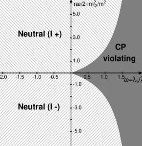
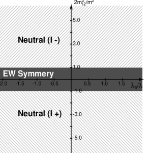
Figure 2: Vacuum states in the plane ${\varkappa}r=2m_{12}^{2}/m^{2}$ (vertical axis) — ${\varkappa}=\lambda_{5}/\lambda$ (horizontal axis). Left plot: $m^{2}>0$, right plot: $m^{2}<0$.

$\bullet$  Comparison of extrema. Vacuum state.

Taking into account the positivity constraint (45b), we note that the condition $r^{2}<1$ is necessary for realization of the charged extremum and type II CPc extremum. It is sufficient for realization of the sCPv extremum as well.

At different parameters of potential different extrema realize the vacuum state (with lowest energy) at$\Delta=\delta=0$. In particular,

$$\begin{array}[]{c}{\cal E}_{CPv}\!-\!{\cal E}_{I}\!=\!-\!{\varepsilon}\,{\varkappa}\dfrac{{(({\varkappa}\!-\!2)r\pm 4)^{2}}}{{4(4-{\varkappa}^{2})}},\\[5.69054pt] {\cal E}_{ch}\!-\!{\cal E}_{CPv}\!=\!{\varepsilon}\,{\varkappa}\left(\!-\!\dfrac{{r^{2}}}{{4}}\!+\!\dfrac{{1}}{{2\!-\!{\varkappa}}}\right).\end{array}$$ (63)

In the region where the charged extremum or CPc extremum II can exist, the sCPv extremum exists too. In this regions we have ${\cal E}_{ch}-{\cal E}_{CPv}>0$ and${\cal E}_{II}-{\cal E}_{CPv}>0$. Therefore in the toy model the charged extremum and type II CPc extremum cannot be vacuum states.

Now one must consider interrelation between the sCPv extremum and type I CPc extrema.

According to (63), at ${\varkappa}<0$ the difference ${\cal E}_{CPv}-{\cal E}_{I}>0$, so the CPc extremum type I is realized in this region. On the other hand, at ${\varkappa}>0$ the difference ${\cal E}_{CPv}-{\cal E}_{I}<0$, but the region where sCPv extremum exists is also constrained by eq. (49).

Fig. 2 shows regions with different vacuum states on the $({\varkappa},{\varkappa}r)$ plane. The left plot shows different vacua for $m^{2}>0$. The right plot shows vacuum states for $m^{2}<0$. In this case only type I CPc conserving extremum exists in the region constrained by (62). In the region$-2<r\,{\varkappa}<2$, the EW symmetry conserving point $y_{i}=0$ is the only minimum of the potential.

References

- (1) T. D. Lee. Phys. Rev. D 8 1226 (1973)
- (2) J.F. Gunion, H.E. Haber, G. Kane, S. Dawson, The Higgs Hunter’s Guide (Addison-Wesley, Reading, 1990).
- (3) Workshop on CP studies and Non-Standard Higgs Physics. CERN - 2006 - 009.
- (4) I.F. Ginzburg, M. Krawczyk, Phys. Rev. D 72 (2005) 115013; hep-ph/0408011
- (5) J. F. Gunion, H. E. Haber, Phys. Rev. D72 (2005) 095002, hep-ph/0506227; S. Davidson, H. E. Haber, Phys. Rev. D72 (2005) 035004, hep-ph/0504050.
- (6) J. F. Gunion., H. E. Haber. Phys. Rev. D 67 075019 (2003)
- (7) A. Barroso, P.M. Ferreira, R. Santos, J.P. Silva, hep-ph/0507329, hep-ph/0608282 Phys. Rev. D74 (2006) 085016, and references there.
- (8) A. Barroso, P.M. Ferreira, R. Santos, hep-ph/0702098
- (9) I.F. Ginzburg, Acta Phys. Polonica B37 (2006) 1161-1172 (preliminary version in hep-ph/0512102)
- (10) I. P. Ivanov, Phys. Lett. B 632 (2006) 360; Phys. Rev. D75 (2007) 035001
- (11) N. G. Deshpande and E. Ma, Phys. Rev. D 18, 2574 (1978); S. Nie and M. Sher, Phys. Lett. B 449, 89 (1999), hep-ph/9811234; S. Kanemura, T. Kasai and Y. Okada, Phys. Lett. B 471, 182 (1999), hep-ph/9903289; B. M. Kastening, hep-ph/9307224
- (12) I.F. Ginzburg, I.P. Ivanov, Phys. Rev. D 72 (2005) 115010.
- (13) G. Sartori, G. Valente, Ann. Phys. (NY) 319 (2005) 286.
- (14) M. Krawczyk, D. Sokolowska, report at LCWS07
- (15) E. Akhmetzyanova, M. Dolgopolov, M. Dubinin, hep-ph/0405264, Phys. Part. Nucl. 37 (2006) 1285
- (16) See e.g. L.Dolan and R. Jackiv. Phys. Rev. D9 (1973) 1888.
- (17) I.F. Ginzburg, I.P. Ivanov, K.A. Kanishev, in preparation
- (18) Ya.B. Zeldovich, I.Yu. Kobzarev, L.B. Okun. Sov. Phys. JETP 40 (1974) 1.