Astrophysical Accretion as an Analogue Gravity Phenomena

Abstract

Inspite of the remarkable resemblance in between a black hole and an ordinary thermodynamic system, black holes never radiate according to the classical laws of physics. The introduction of quantum effects radically changes the scenario. Black holes radiate due to quantum effects. Such radiation is known as Hawking radiation and the corresponding radiation temperature is referred as the Hawking temperature. Observational manifestation of Hawking effect for astrophysical black holes is beyond the scope of present day’s experimental techniques. Also, Hawking quanta may posses trans-Planckian frequencies, and physics beyond the Planck scale is not well understood. The above mentioned difficulties with Hawking effect were the motivations to search for an analogous version of Hawking radiation, and the theory of acoustic/analogue black holes were thus introduced.

Classical black hole analogues (alternatively, the analogue systems) are fluid dynamical analogue of general relativistic black holes. Such analogue effects may be observed when the acoustic perturbation (sound waves) propagates through a classical dissipation-less transonic fluid. The acoustic horizon, which resembles the actual black hole event horizon in many ways, may be generated at the transonic point in the fluid flow. Acoustic horizon emits acoustic radiation with quasi thermal phonon spectra, which is analogous to the actual Hawking radiation.

Transonic accretion onto astrophysical black holes is a very interesting example of classical analogue system found naturally in the Universe. An accreting black hole system as a classical analogue is unique in the sense that only for such a system, both kind of horizons, the electromagnetic and the acoustic (generated due to transonicity of accreting fluid) are simultaneously present in the same system. Hence accreting astrophysical black holes are the most ideal candidate to study theoretically and to compare the properties of these two different kind of horizons. Such a system is also unique in the aspect that accretion onto the black holes represents the only classical analogue system found in the nature so far, where the analogue Hawking temperature may exceed the actual Hawking temperature. In this review article, it will be demonstrated that, in general, the transonic accretion in astrophysics can be considered as an example of the classical analogue gravity model.

I Black Holes

Black holes are the vacuum solutions of Einstein’s field equations in general relativity. Classically, a black hole is conceived as a singularity in space time, censored from the rest of the Universe by a mathematically defined one way surface, the event horizon. Black holes are completely characterized only by three externally observable parameters, the mass of the black hole $M_{BH}$, the rotation (spin) $J_{BH}$ and charge $Q_{BH}$. All other informations about the matter which formed the black hole or is falling into it, disappear behind the event horizon, are therefore permanently inaccessible to the external observer. Thus the space time metric defining the vacuum exterior of a classical black hole is characterized by $M_{BH},J_{BH}$ and $Q_{BH}$ only. The most general family of black hole solutions have non zero values of $M_{BH},J_{BH}$ and $Q_{BH}$ (rotating charged black holes), and are known as the Kerr-Newman black holes. The following table classifies various categories of black hole solutions according to the value of $M_{BH},J_{BH}$ and $Q_{BH}$.

Types of Black Hole	Mass	Angular Momentum	Charge
Kerr-Newman
(Newman et. al. 1965)	${\bf M}_{\bf BH}>{\bf 0}$	${\bf J}_{\bf BH}{\neq}{\bf 0}$	${\bf Q}_{\bf BH}{\neq}{\bf 0}$
Kerr (Kerr 1963)	${\bf M}_{\bf BH}>{\bf 0}$	${\bf J}_{\bf BH}{\neq}{\bf 0}$	${\bf Q}_{\bf BH}{=}{\bf 0}$
Reissner-Nordstr$\ddot{\rm o}$m
(Reissner 1916; Weyl 1917; Nordstr$\ddot{o}$m 1918)	${\bf M}_{\bf BH}>{\bf 0}$	${\bf J}_{\bf BH}{=}{\bf 0}$	${\bf Q}_{\bf BH}{\neq}{\bf 0}$
Schwarzschild
(Schwarzschild 1916)	${\bf M}_{\bf BH}>{\bf 0}$	${\bf J}_{\bf BH}{=}{\bf 0}$	${\bf Q}_{\bf BH}{=}{\bf 0}$

Table 1: Classification of black holes according to the value of its Mass, angular momentum and charge.

The Israle-Carter-Robinson theorem (Israle 1967; Carter 1971; Robinson 1975), when coupled with Price’s conjecture (Price 1972), ensures that any object with event horizon must rapidly settles down to the Kerr metric, radiating away all its irregularities and distortions which may deviate them from the black hole solutions exactly described by the Kerr metric.

In astrophysics, black holes are the end point of gravitational collapse of massive celestial objects. The Kerr-Newman and the Reissner-Nordstr$\ddot{\rm o}$m black hole solutions usually do not play any significant role in astrophysical context. Typical astrophysical black holes are supposed to be immersed in an charged plasma environment. Any net charge $Q_{BH}$ will thus rapidly be neutrilized by teh ambient magnetic field. The time scale for such charge relaxation would be roughly of the order of $\left(M_{BH}/M_{\odot}\right){\mu}{\rm sec}$ ($M_{\odot}$ being the mass of the Sun, see, e.g., Hughes 2005 for further details), which is obviously far shorter compared to the rather long timescale relevant to observing most of the properties of the astrophysical black holes. Hence the Kerr solution provides the complete description of most stable astrophysical black holes. However, the study of Schwarzschild black holes, although less general compared to the Kerr type holes, is still greatly relevant in astrophysics.

Astrophysical black holes may be broadly classified into two categories, the stellar mass ($M_{BH}{\sim}$ a few $M_{\odot}$), and super massive ($M_{BH}{\geq}{10^{6}}M_{\odot}$) black holes. While the birth history of the stellar mass black holes is theoretically known with almost absolute certainty (they are the endpoint of the gravitational collapse of massive stars), the formation scenario of the supermassive black hole is not unanimously understood. A super massive black hole may form through the monolithic collapse of early proto-spheroid gaseous mass originated at the time of galaxy formation. Or a number of stellar/intermediate mass black holes may merge to form it. Also the runaway growth of a seed black hole by accretion in a specially favoured high-density environment may lead to the formation of super massive black holes. However, it is yet to be well understood exactly which of the above mentioned processes routes toward the formation of super massive black holes; see, e.g., Rees 1984, 2002; Haiman & Quataert 2004; and Volonteri 2006, for comprehensive review on the formation and evolution of super massive black holes.

Both kind of astrophysical black holes, the stellar mass and super massive black holes, however, accrete matter from the surroundings. Depending on the intrinsic angular momentum content of accreting material, either spherically symmetric (zero angular momentum flow of matter), or axisymmetric (matter flow with non-zero finite angular momentum) flow geometry is invoked to study an accreting black hole system (see the excellent monographs by Frank, King & Raine 1992, and Kato, Fukue & Mineshige 1998, for details about the astrophysical accretion processes). We will get back to the accretion process in greater detail in subsequent sections.

II Black Hole Thermodynamics

Within the framework of purely classical physics, black holes in any diffeomorphism covariant theory of gravity (where the field equations directly follow from the diffeomorphism covariant Lagrangian) and in general relativity, mathematically resembles some aspects of classical thermodynamic systems (Wald 1984, 1994, 2001; Keifer 1998; Brown 1995, and references therein). In early seventies, a series of influential works (Bekenstein 1972, 1972a, 1973, 1975; Israel 1976; Bardeen, Carter & Hawking 1973, see also Bekenstein 1980 for a review) revealed the idea that classical black holes in general relativity, obey certain laws which bear remarkable analogy to the ordinary laws of classical thermodynamics. Such analogy between black hole mechanics and ordinary thermodynamics (‘The Generalized Second Law’, as it is customarily called) leads to the idea of the ‘surface gravity’ of black hole, $\kappa$, which can be obtained by computing the norm of the gradient of the norms of the Killing fields evaluated at the stationary black hole horizon, and is found to be constant on the horizon (analogous to the constancy of temperature T on a body in thermal equilibrium - the ‘Zeroth Law’ of classical thermodynamics). Also, $\kappa=0$ can not be accomplished by performing finite number of operations (analogous to the ‘weak version’ of the third law of classical thermodynamics where temperature of a system cannot be made to reach at absolute zero, see discussions in Keifer 1998). It was found by analogy via black hole uniqueness theorem (see, e.g., Heusler 1996, and references therein) that the role of entropy in classical thermodynamic system is played by a constant multiple of the surface area of a classical black hole.

III Hawking Radiation

The resemblance between the laws of ordinary thermodynamics to those of black hole mechanics were, however, initially regarded as purely formal. This is because, the physical temperature of a black hole is absolute zero (see, e.g. Wald 2001). Hence physical relationship between the surface gravity of the black hole and the temperature of a classical thermodynamic system can not be conceived. This further indicates that a classical black hole can never radiate. However, introduction of quantum effects might bring a radical change to the situation. In an epoch making paper published in 1975, Hawking (Hawking 1975) used quantum field theoretic calculation on curved spacetime to show that the physical temperature and entropy of black hole does have finite non-zero value (see Page 2004 and Padmanabhan 2005 for intelligible reviews of black hole thermodynamics and Hawking radiation). A classical space time describing gravitational collapse leading to the formation of a Schwarzschild black hole was assumed to be the dynamical back ground, and a linear quantum field, initially in it’s vacuum state prior to the collapse, was considered to propagate against this background. The vacuum expectation value of the energy momentum tensor of this field turned out to be negative near the horizon. This phenomenon leads to the flux of negative energy into the hole. Such negative energy flux would decrease the mass of the black hole and would lead to the fact that the quantum state of the outgoing mode of the field would contain particles. The expected number of such particles would correspond to radiation from a perfect black body of finite size. Hence the spectrum of such radiation is thermal in nature, and the temperature of such radiation, the Hawking temperature $T_{H}$ from a Schwarzschild black hole, can be computed as

$$T_{H}=\frac{{\hbar}c^{3}}{8{\pi}k_{B}GM_{BH}}$$ (1)

where $G$ is the universal gravitational constant, $c,{\hbar}$ and $k_{B}$ are the velocity of light in vacuum, the Dirac’s constant and the Boltzmann’s constant, respectively.

The semi classical description for Hawking radiation treats the gravitational field classically and the quantized radiation field satisfies the d’Alembert equation. At any time, black hole evaporation is an adiabatic process if the residual mass of the hole at that time remains larger than the Planck mass.

IV Toward an Analogy of Hawking Effect

Substituting the values of the fundamental constants in Eq. (1), one can rewrite $T_{H}$ for a Schwarzschild black hole as (Helfer 2003):

$$T_{H}~{}{\sim}~{}6.2{\times}10^{-8}\left(\frac{M_{\odot}}{M_{BH}}\right){\rm Degree~{}~{}Kelvin}$$ (2)

It is evident from the above equation that for one solar mass black hole, the value of the Hawking temperature would be too small to be experimentally detected. A rough estimate shows that $T_{H}$ for stellar mass black holes would be around $10^{7}$ times colder than the cosmic microwave background radiation. The situation for super massive black hole will be much more worse, as $T_{H}{\propto}{1}/{M_{BH}}$. Hence $T_{H}$ would be a measurable quantity only for primordial black holes with very small size and mass, if such black holes really exist, and if instruments can be fabricated to detect them. The lower bound of mass for such black holes may be estimated analytically. The time-scale ${\cal T}$ (in years) over which the mass of the black hole changes significantly due to the Hawking’s process may be obtained as (Helfer 2003):

$${\cal T}{\sim}\left(\frac{M_{BH}}{M_{\odot}}\right)^{3}10^{65}~{}~{}{\rm Years}$$ (3)

As the above time scale is a measure of the lifetime of the hole itself, the lower bound for a primordial hole may be obtained by setting ${\cal T}$ equal to the present age of the Universe. Hence the lower bound for the mass of the primordial black holes comes out to be around $10^{15}$ gm. The size of such a black hole would be of the order of $10^{-13}$ cm and the corresponding $T_{H}$ would be about $10^{11}{\rm K}$, which is comparable with the macroscopic fluid temperature of the freely falling matter (spherically symmetric accretion) onto an one solar mass isolated Schwarzschild black hole (see section 12.1 for further details). However, present day instrumental technique is far from efficient to detect these primordial black holes with such an extremely small dimension, if such holes exist at all in first place. Hence, the observational manifestation of Hawking radiation seems to be practically impossible.

On the other hand, due to the infinite redshift caused by the event horizon, the initial configuration of the emergent Hawking Quanta is supposed to possess trans-Planckian frequencies and the corresponding wave lengths are beyond the Planck scale. Hence, low energy effective theories cannot self consistently deal with the Hawking radiation (see, e.g., Parentani 2002 for further details). Also, the nature of the fundamental degrees of freedom and the physics of such ultra short distance is yet to be well understood. Hence, some of the fundamental issues like the statistical meaning of the black hole entropy, or the exact physical origin of the out going mode of the quantum field, remains unresolved (Wald 2001).

Perhaps the above mentioned difficulties associated with the theory of Hawking radiation served as the principal motivation to launch a theory, analogous to the Hawking’s one, effects of which would be possible to comprehend through relatively more perceivable physical systems. The theory of analogue Hawking radiation opens up the possibility to experimentally verify some basic features of black hole physics by creating the sonic horizons in the laboratory. A number of works have been carried out to formulate the condensed matter or optical analogue of event horizons . The theory of analogue Hawking radiation may find important uses in the fields of investigation of quasi-normal modes (Berti, Cardoso & Lemos 2004; Cardoso, Lemos & Yoshida 2004), acoustic super-radiance (Basak & Majumdar 2003; Basak 2005; Lepe & Saavedra 2005; Slatyer, & Savage 2005; Cherubini, Federici & Succi 2005; Kim, Son, & Yoon 2005; Choy, Kruk, Carrington, Fugleberg, Zahn, Kobes, Kunstatter & Pickering 2005; Federici, Cherubini, Succi & Tosi 2005), FRW cosmology (Barcelo, Liberati & Visser 2003) inflationary models, quantum gravity and sub-Planckian models of string theory (Parentani 2002).

For space limitation, in this article, we will, however, mainly describe the formalism behind the classical analogue systems. By ‘classical analogue systems’ we refer to the examples where the analogue effects are studied in classical systems (fluids), and not in quantum fluids. In the following sections, we discuss the basic features of a classical analogue system.

V Analogue Gravity Model and the Black Hole Analogue

In recent years, strong analogies have been established between the physics of acoustic perturbations in an inhomogeneous dynamical fluid system, and some kinematic features of space-time in general relativity. An effective metric, referred to as the ‘acoustic metric’, which describes the geometry of the manifold in which acoustic perturbations propagate, can be constructed. This effective geometry can capture the properties of curved space-time in general relativity. Physical models constructed utilizing such analogies are called ‘analogue gravity models’ (for details on analogue gravity models, see, e.g. the review articles by Barcelo, Liberati & Visser (2005) and Cardoso (2005), and the monograph by Novello, Visser & Volovik (2002)).

One of the most significant effects of analogue gravity is the ‘classical black hole analogue’. Classical black hole analogue effects may be observed when acoustic perturbations (sound waves) propagate through a classical, dissipation-less, inhomogeneous transonic fluid. Any acoustic perturbation, dragged by a supersonically moving fluid, can never escape upstream by penetrating the ‘sonic surface’. Such a sonic surface is a collection of transonic points in space-time, and can act as a ‘trapping’ surface for outgoing phonons. Hence, the sonic surface is actually an acoustic horizon, which resembles a black hole event horizon in many ways and is generated at the transonic point in the fluid flow. The acoustic horizon is essentially a null hyper surface, generators of which are the acoustic null geodesics, i.e. the phonons. The acoustic horizon emits acoustic radiation with quasi thermal phonon spectra, which is analogous to the actual Hawking radiation. The temperature of the radiation emitted from the acoustic horizon is referred to as the analogue Hawking temperature.

Hereafter, we shall use $T_{{AH}}$ to denote the analogue Hawking temperature, and $T_{H}$ to denote the the actual Hawking temperature as defined in (1). We shall also use the words ‘analogue’, ‘acoustic’ and ‘sonic’ synonymously in describing the horizons or black holes. Also the phrases ‘analogue (acoustic) Hawking radiation/effect/temperature’ should be taken as identical in meaning with the phrase ‘analogue (acoustic) radiation/effect/temperature’. A system manifesting the effects of analogue radiation, will be termed as analogue system.

In a pioneering work, Unruh (1981) showed that a classical system, relatively more clearly perceivable than a quantum black hole system, does exist, which resembles the black hole as far as the quantum thermal radiation is concerned. The behaviour of a linear quantum field in a classical gravitational field was simulated by the propagation of acoustic disturbance in a convergent fluid flow. In such a system, it is possible to study the effect of the reaction of the quantum field on it’s own mode of propagation and to contemplate the experimental investigation of the thermal emission mechanism. Considering the equation of motion for a transonic barotropic irrotational fluid, Unruh (1981) showed that the scaler field representing the acoustic perturbation (i.e, the propagation of sound wave) satisfies a differential equation which is analogous to the equation of a massless scaler field propagating in a metric. Such a metric closely resembles the Schwarzschild metric near the horizon. Thus acoustic propagation through a supersonic fluid forms an analogue of event horizon, as the ‘acoustic horizon’ at the transonic point. The behaviour of the normal modes near the acoustic horizon indicates that the acoustic wave with a quasi-thermal spectrum will be emitted from the acoustic horizon and the temperature of such acoustic emission may be calculated as (Unruh 1981):

$$T_{AH}=\frac{\hbar}{4{\pi}k_{B}}\left[\frac{1}{c_{s}}\frac{{\partial}{u_{\perp}^{2}}}{\partial{\eta}}\right]_{\rm r_{h}}$$ (4)

Where $r_{h}$ represents the location of the acoustic horizon, $c_{s}$ is the sound speed, $u_{\perp}$ is the component of the dynamical flow velocity normal to the acoustic horizon, and ${\partial}/{{\partial}{\eta}}$ represents derivative in the direction normal to the acoustic horizon.

Equation (4) has clear resemblance with (1) and hence $T_{AH}$ is designated as analogue Hawking temperature and such quasi-thermal radiation from acoustic (analogue) black hole is known as the analogue Hawking radiation. Note that the sound speed $c_{s}$ in Unruh’s original treatment (the above equation) was assumed to be constant in space, i.e., an isothermal equation of state had been invoked to describe the fluid.

Unruh’s work was followed by other important papers (Jacobson 1991, 1999; Unruh 1995; Visser 1998; Bili$\acute{c}$ 1999) A more general treatment of the classical analogue radiation for Newtonian fluid was discussed by Visser (1998), who considered a general barotropic, inviscid fluid. The acoustic metric for a point sink was shown to be conformally related to the Painlevé-Gullstrand-Lemaître form of the Schwarzschild metric (Painlevé 1921; Gullstrand 1922; Lemaître 1933) and a more general expression for analogue temperature was obtained, where unlike Unruh’s original expression (4), the speed of sound was allowed to depend on space coordinates.

In the analogue gravity systems discussed above, the fluid flow is non-relativistic in flat Minkowski space, whereas the sound wave propagating through the non-relativistic fluid is coupled to a curved pseudo-Riemannian metric. This approach has been extended to relativistic fluids (Bili$\acute{c}$ 1999) by incorporating the general relativistic fluid dynamics.

In subsequent sections, we will pedagogically develop the concept of the acoustic geometry and related quantities, like the acoustic surface gravity and the acoustic Hawking temperature.

VI Curved Acoustic Geometry in a Flat Space-time

Let $\psi$ denote the velocity potential describing the fluid flow in Newtonian space-time, i.e. let ${\vec{u}}=-{\nabla}\psi$, where ${\vec{u}}$ is the velocity vector describing the dynamics of a Newtonian fluid. The specific enthalpy $h$ of a barotropic Newtonian fluid satisfies ${\nabla}h=(1/{\rho}){\nabla}p$, where $\rho$ and $p$ are the density and the pressure of the fluid. One then writes the Euler equation as

$$-{\partial}_{t}{\psi}+h+\frac{1}{2}\left({\nabla}{\psi}\right)^{2}+\Phi=0,$$ (5)

where $\Phi$ represents the potential associated with any external driving force. Assuming small fluctuations around some steady background $\rho_{0},p_{0}$ and $\psi_{0}$, one can linearize the continuity and the Euler equations and obtain a wave equation (see Landau & Lifshitz 1959, and Visser 1998, for further detail).

The continuity and Euler’s equations may be expressed as:

$$\frac{\partial{\rho}}{\partial{t}}+{\nabla}\cdot\left(\rho{\vec{u}}\right)$$ (6)

$$\rho\frac{d{\vec{u}}}{dt}{\equiv}\rho\left[\frac{\partial{\vec{u}}}{\partial{t}}+\left({\vec{u}}\cdot{\nabla}\right){\vec{u}}\right]=-\nabla{p}+{\vec{F}}$$ (7)

with ${\vec{F}}$ being the sum of all external forces acting on the fluid which may be expressed in terms of a potential

$${\vec{F}}=-{\rho}{\nabla}{\Phi},$$ (8)

Euler’s equation may now be recast in the form

$$\frac{\partial{\vec{u}}}{\partial{t}}={\vec{u}}\times(\nabla\times{\vec{u}})-{1\over\rho}\nabla p-\nabla\left({{1\over 2}}u^{2}+\Phi\right)$$ (9)

Next we assume the fluid to be inviscid, irrotational, and barotropic. Introducing the specific enthalpy $h$, such that

$${\nabla}h=\frac{\nabla{p}}{\rho}$$ (10)

and the velocity potential $\psi$ for which ${\vec{u}}=-{\nabla}\psi$, Eq. (9) may be written as

$$-\frac{\partial{\psi}}{\partial{t}}+h+{1\over 2}(\nabla\psi)^{2}+\Phi=0$$ (11)

One now linearizes the continuity and Euler’s equation around some unperturbed background flow variables $\rho_{0}$, $p_{0}$, $\psi_{0}$. Introducing

$$\rho=\rho_{0}+\epsilon\rho_{1}+{\cal O}(\epsilon^{2}), p=p_{0}+\epsilon p_{1}+{\cal O}(\epsilon^{2}),$$

$$\psi=\psi_{0}+\epsilon\psi_{1}+{\cal O}(\epsilon^{2}), h=h_{0}+\epsilon h_{1},$$ (12)

from the continuity equation we obtain

$$\frac{\partial\rho_{0}}{\partial{t}}+\nabla\cdot(\rho_{0}\;{\vec{u}}_{0})=0;\;\;\;\;\;\frac{\partial\rho_{1}}{\partial{t}}+\nabla\cdot(\rho_{1}\;{\vec{u}}_{0}+\rho_{0}\;{\vec{u}}_{1})=0.$$ (13)

Equation (10) implies

$$h_{1}=p_{1}\frac{dh}{dp}=\frac{p_{1}}{\rho_{0}}\,.$$ (14)

Using this the linearized Euler equation reads

$$-\frac{\partial{\psi_{0}}}{\partial{t}}+h_{0}+{1\over 2}(\nabla\psi_{0})^{2}+\Phi=0;\;\;\;\;\;-\frac{\partial{\psi_{0}}}{\partial{t}}+{p_{1}\over\rho_{1}}-{\vec{u}}_{0}\cdot\nabla\psi_{1}=0.$$ (15)

Re-arrangement of the last equation together with the barotropic assumption yields

$$\rho_{1}={\partial\rho\over\partial p}\;p_{1}={\partial\rho\over\partial p}\;\rho_{0}\;(\partial_{t}\psi_{1}+{\vec{u}}_{0}\cdot\nabla\psi_{1})\,.$$ (16)

Substitution of this into the linearized continuity equation gives the sound wave equation

$$-\frac{\partial}{\partial{t}}\left[{\partial\rho\over\partial p}\;\rho_{0}\;\left(\frac{\partial\psi_{1}}{\partial{t}}+{\vec{u}}_{0}\cdot\nabla\psi_{1}\right)\right]+\nabla\cdot\left[\rho_{0}\;\nabla\psi_{1}-{\partial\rho\over\partial p}\;\rho_{0}\;{\vec{v}}_{0}\;\left(\frac{\partial\psi_{1}}{\partial{t}}+{\vec{v}}_{0}\cdot\nabla\psi_{1}\right)\right]=0.$$ (17)

Next, we define the local speed of sound by

$$c_{s}^{2}={\partial{p}}/{\partial\rho},$$ (18)

where the partial derivative is taken at constant specific entropy. With help of the $4\times{4}$ matrix

$$f^{\mu\nu}\equiv{\rho^{0}}\left[\matrix{-{I}&\vdots&-{\vec{u}}\cr\cdots\cdots&\cdot&\cdots\cdots\cdots\cdots\cr-{\vec{u}}&\vdots&(c_{s}^{2}-{{u}^{2}})\cr}\right]$$ (19)

where ${I}$ is the $3\times 3$ identity matrix, one can put Eq. (17) to the form

$${\partial}_{\mu}\left(f^{\mu{\nu}}{\partial}_{\nu}{\psi^{1}}\right)=0.$$ (20)

Equation (20) describes the propagation of the linearized scalar potential $\psi^{1}$. The function $\psi^{1}$ represents the low amplitude fluctuations around the steady background $(\rho_{0},p_{0},\psi_{0})$ and thus describes the propagation of acoustic perturbation, .i.e. the propagation of sound waves.

The form of Eq. (20) suggests that it may be regarded as a d’Alembert equation in curved space-time geometry. In any pseudo-Riemannian manifold the d’Alembertian operator can be expressed as (Misner, Thorne & Wheeler 1973)

$$\Box=\frac{1}{\sqrt{-\left|g_{\mu{\nu}}\right|}}{\partial}_{\mu}{\sqrt{-\left|g_{\mu{\nu}}\right|}}g^{\mu{\nu}}{\partial}_{\nu}\,,$$ (21)

where $\left|g_{\mu{\nu}}\right|$ is the determinant and $g^{\mu{\nu}}$ is the inverse of the metric $g_{\mu{\nu}}$. Next, if one identifies

$$f^{\mu{\nu}}=\sqrt{-\left|g_{\mu{\nu}}\right|}g^{{\mu}\nu},$$ (22)

one can recast the acoustic wave equation in the form (Visser 1998)

$$\frac{1}{\sqrt{-\left|G_{\mu{\nu}}\right|}}{\partial}_{\mu}\left({\sqrt{-\left|G_{\mu{\nu}}\right|}}G^{\mu{\nu}}\right){\partial_{\nu}}\psi^{1}=0,$$ (23)

where $G_{\mu{\nu}}$ is the acoustic metric tensor for the Newtonian fluid. The explicit form of ${G}_{\mu{\nu}}$ is obtained as

$$G_{\mu\nu}\equiv{\rho_{0}}\left[\matrix{-(c_{s}^{2}-u^{2})&\vdots&-{{\vec{u}}}\cr\cdots\cdots\cdots\cdots&\cdot&\cdots\cdots\cr-{\vec{u}}&\vdots&{I}\cr}\right]$$ (24)

The Lorentzian metric described by (24) has an associated non-zero acoustic Riemann tensor for non-homogeneous, flowing fluids.

Thus, the propagation of acoustic perturbation, or the sound wave, embedded in a barotropic, irrotational, non-dissipative Newtonian fluid flow may be described by a scalar d’Alembert equation in a curved acoustic geometry. The corresponding acoustic metric tensor is a matrix that depends on dynamical and thermodynamic variables parameterizing the fluid flow.

For analogue systems discussed above, the fluid particles are coupled to the flat metric of Mankowski’s space (because the governing equation for fluid dynamics in the above treatment is completely Newtonian), whereas the sound wave propagating through the non-relativistic fluid is coupled to the curved pseudo-Riemannian metric. Phonons (quanta of acoustic perturbations) are the null geodesics, which generate the null surface, i.e., the acoustic horizon. Introduction of viscosity may destroy the Lorentzian invariance and hence the acoustic analogue is best observed in a vorticity free completely dissipation-less fluid (Visser 1998, and references therein). That is why, the Fermi superfluids and the Bose-Einstein condensates are ideal to simulate the analogue effects.

The most important issue emerging out of the above discussions is that (see Visser 1998 and Barcelo, Liberati & Visser 2005 for further details): Even if the governing equation for fluid flow is completely non-relativistic (Newtonian), the acoustic fluctuations embedded into it are described by a curved pseudo-Riemannian geometry. This information is useful to portray the immense importance of the study of the acoustic black holes, i.e. the black hole analogue, or simply, the analogue systems.

The acoustic metric (24) in many aspects resembles a black hole type geometry in general relativity. For example, the notions such as ‘ergo region’ and ‘horizon’ may be introduced in full analogy with those of general relativistic black holes. For a stationary flow, the time translation Killing vector $\xi\equiv\partial/\partial t$ leads to the concept of acoustic ergo sphere as a surface at which $G_{\mu\nu}\xi^{\mu}\xi^{\nu}$ changes its sign. The acoustic ergo sphere is the envelop of the acoustic ergo region where $\xi^{\mu}$ is space-like with respect to the acoustic metric. Through the equation $G_{\mu\nu}\xi^{\mu}\xi^{\nu}=g_{tt}=u^{2}-c_{s}^{2}$, it is obvious that inside the ergo region the fluid is supersonic. The ‘acoustic horizon’ can be defined as the boundary of a region from which acoustic null geodesics or phonons, cannot escape. Alternatively, the acoustic horizon is defined as a time like hypersurface defined by the equation

$$c_{s}^{2}-u_{\perp}^{2}=0,$$ (25)

where $u_{\perp}$ is the component of the fluid velocity perpendicular to the acoustic horizon. Hence, any steady supersonic flow described in a stationary geometry by a time independent velocity vector field forms an ergo-region, inside which the acoustic horizon is generated at those points where the normal component of the fluid velocity is equal to the speed of sound.

In analogy to general relativity, one also defines the surface gravity and the corresponding Hawking temperature associated with the acoustic horizon. The acoustic surface gravity may be obtained (Wald 1984) by computing the gradient of the norm of the Killing field which becomes null vector field at the acoustic horizon. The acoustic surface gravity $\kappa$ for a Newtonian fluid is then given by (Visser 1998)

$$\kappa=\frac{1}{2c_{s}}\left|\frac{\partial}{\partial\eta}\left(c_{s}^{2}-u_{\perp}^{2}\right)\right|\,.$$ (26)

The corresponding Hawking temperature is then defined as usual:

$$T_{AH}=\frac{\kappa}{2\pi\kappa_{B}}\,.$$ (27)

VII Curved Acoustic Geometry in a Curved Space-time

The above formalism may be extended to relativistic fluids in curved space-time background (Bilić 1999). The propagation of acoustic disturbance in a perfect relativistic inviscid irrotational fluid is also described by the wave equation of the form (23) in which the acoustic metric tensor and its inverse are defined as (Bilić 1999; Abraham, Bilić & Das 2006; Das, Bilić & Dasgupta 2006)

$${G}_{\mu\nu}=\frac{\rho}{hc_{s}}\left[g_{\mu\nu}+(1-c_{s}^{2})v_{\mu}v_{\nu}\right];\;\;\;\;G^{\mu\nu}=\frac{hc_{s}}{\rho}\left[g^{\mu\nu}+(1-\frac{1}{c_{s}^{2}})v^{\mu}v^{\mu}\right],$$ (28)

where $\rho$ and $h$ are, respectively, the rest-mass density and the specific enthalpy of the relativistic fluid, $v^{\mu}$ is the four-velocity, and $g_{\mu\nu}$ the background space-time metric. A ($-,+++$) signature has been used to derive (28). The ergo region is again defined as the region where the stationary Killing vector $\xi$ becomes spacelike and the acoustic horizon as a timelike hypersurface the wave velocity of which equals the speed of sound at every point. The defining equation for the acoustic horizon is again of the form (25) in which the three-velocity component perpendicular to the horizon is given by

$$u_{\perp}=\frac{\left(\eta^{\mu}v_{\mu}\right)^{2}}{\left(\eta^{\mu}{v_{\mu}}\right)^{2}+\eta^{\mu}\eta_{\mu}},$$ (29)

where $\eta^{\mu}$ is the unit normal to the horizon. For further details about the propagation of the acoustic perturbation, see Abraham, Bilić & Das 2006.

It may be shown that, the discriminant of the acoustic metric for an axisymmetric flow

$${\cal D}=G_{t\phi}^{2}-G_{tt}G_{\phi\phi},$$ (30)

vanishes at the acoustic horizon. A supersonic flow is characterized by the condition ${\cal D}>0$, whereas for a subsonic flow, ${\cal D}<0$ (Abraham, Bilić & Das 2006). According to the classification of Bercelo, Liberati, Sonego & Visser (2004), a transition from a subsonic (${\cal D}<0$) to a supersonic (${\cal D}>0$) flow is an acoustic black hole, whereas a transition from a supersonic to a subsonic flow is an acoustic white hole.

For a stationary configuration, the surface gravity can be computed in terms of the Killing vector

$$\chi^{\mu}=\xi^{\mu}+\Omega\phi^{\mu}$$ (31)

that is null at the acoustic horizon. Following the standard procedure (Wald 1984; Bilić 1999) one finds that the expression

$$\kappa\chi^{\mu}=\frac{1}{2}G^{\mu\nu}\eta_{\nu}\frac{\partial}{\partial{\eta}}(G_{\alpha\beta}\chi^{\alpha}\chi{\beta})$$ (32)

holds at the acoustic horizon, where the constant $\kappa$ is the surface gravity. From this expression one deduces the magnitude of the surface gravity as (see Bilić 1999; Abraham, Bilić & Das 2006; Das, Bilić & Dasgupta 2006 for further details)

$$\kappa=\left|\frac{\sqrt{-{\chi}^{\nu}{\chi}_{\nu}}}{1-c_{s}^{2}}\frac{\partial}{\partial{\eta}}\left(u-c_{s}\right)\right|_{\rm r=r_{h}}$$ (33)

VIII Quantization of Phonons and the Hawking Effect

The purpose of this section (has been adopted from Das, Bilić & Dasgupta 2006) is to demonstrate how the quantization of phonons in the presence of the acoustic horizon yields acoustic Hawking radiation. The acoustic perturbations considered here are classical sound waves or phonons that satisfy the massless wave equation in curved background, i.e. the general relativistic analogue of (23), with the metric $G_{\mu\nu}$ given by (28). Irrespective of the underlying microscopic structure, acoustic perturbations are quantized. A precise quantization scheme for an analogue gravity system may be rather involved (Unruh & Sch$\ddot{\rm u}$tzhold 2003). However, at the scales larger than the atomic scales below which a perfect fluid description breaks down, the atomic substructure may be neglected and the field may be considered elementary. Hence, the quantization proceeds in the same way as in the case of a scalar field in curved space (Birrell & Davies 1982) with a suitable UV cutoff for the scales below a typical atomic size of a few Å.

For our purpose, the most convenient quantization prescription is the Euclidean path integral formulation. Consider a 2+1-dimensional axisymmetric geometry describing the fluid flow (since we are going to apply this on the equatorial plane of the axisymmetric black hole accretion disc, see section 13 for further details). The equation of motion (23) with (28) follows from the variational principle applied to the action functional

$$S[\varphi]=\int dtdrd\phi\,\sqrt{-G}\,G^{\mu\nu}\partial_{\mu}\varphi\partial_{\nu}\varphi\,.$$ (34)

We define the functional integral

$$Z=\int{\cal D}\varphi e^{-S_{\rm E}[\varphi]},$$ (35)

where $S_{\rm E}$ is the Euclidean action obtained from (34) by setting $t=i\tau$ and continuing the Euclidean time $\tau$ from imaginary to real values. For a field theory at zero temperature, the integral over $\tau$ extends up to infinity. Here, owing to the presence of the acoustic horizon, the integral over $\tau$ will be cut at the inverse Hawking temperature $2\pi/\kappa$ where $\kappa$ denotes the analogue surface gravity. To illustrate how this happens, consider, for simplicity, a non-rotating fluid ($v_{\phi}=0$) in the Schwarzschild space-time. It may be easily shown that the acoustic metric takes the form

$$ds^{2}=g_{tt}\frac{c_{s}^{2}-u^{2}}{1-u^{2}}dt^{2}-2u\frac{1-c_{s}^{2}}{1-u^{2}}drdt-\frac{1}{g_{tt}}\frac{2-c_{s}^{2}u^{2}}{1-u^{2}}dr^{2}+r^{2}d\phi^{2}\,,$$ (36)

where $g_{tt}=-(1-2/r)$, $u=|v_{r}|/\sqrt{-g_{tt}}$, and we have omitted the irrelevant conformal factor $\rho/(hc_{s})$. Using the coordinate transformation

$$dt\rightarrow dt+\frac{u}{g_{tt}}\frac{1-c_{s}^{2}}{c_{s}^{2}-u^{2}}dr$$ (37)

we remove the off-diagonal part from (36) and obtain

$$ds^{2}=g_{tt}\frac{c_{s}^{2}-u^{2}}{1-u^{2}}dt^{2}-\frac{1}{g_{tt}}\left[\frac{2-c_{s}^{2}u^{2}}{1-u^{2}}+\frac{u^{2}(1-c_{s}^{2})^{2}}{(c_{s}^{2}-u^{2})(1-u^{2})}\right]dr^{2}+r^{2}d\phi^{2}.$$ (38)

Next, we evaluate the metric near the acoustic horizon at $r=r_{\rm h}$ using the expansion in $r-r_{\rm h}$ at first order

$$c_{s}^{2}-u^{2}\approx 2c_{s}\left.\frac{\partial}{\partial r}(c_{s}-u)\right|_{r_{\rm h}}(r-r_{\rm h})$$ (39)

and making the substitution

$$r-r_{\rm h}=\frac{-g_{tt}}{2c_{s}(1-c_{s}^{2})}\left.\frac{\partial}{\partial r}(c_{s}-u)\right|_{r_{\rm h}}R^{2},$$ (40)

where $R$ denotes a new radial variable. Neglecting the first term in the square brackets in (38) and setting $t=i\tau$, we obtain the Euclidean metric in the form

$$ds_{\rm E}^{2}=\kappa^{2}R^{2}d\tau^{2}+dR^{2}+r_{\rm h}^{2}d\phi^{2}\,,$$ (41)

where

$$\kappa=\frac{-g_{tt}}{1-c_{s}^{2}}\left|\frac{\partial}{\partial r}(u-c_{s})\right|_{r_{\rm h}}\,.$$ (42)

Hence, the metric near $r=r_{\rm h}$ is the product of the metric on S¹ and the Euclidean Rindler space-time

$$ds_{\rm E}^{2}=dR^{2}+R^{2}d(\kappa\tau)^{2}.$$ (43)

With the periodic identification $\tau\equiv\tau+2\pi/\kappa$, the metric (43) describes $\Re^{2}$ in plane polar coordinates.

Furthermore, making the substitutions $R=e^{\kappa x}/\kappa$ and $\phi=y/r_{\rm h}+\pi$, the Euclidean action takes the form of the 2+1-dimensional free scalar field action at non-zero temperature

$$S_{\rm E}[\varphi]=\int_{0}^{2\pi/\kappa}d\tau\int_{-\infty}^{\infty}dx\int_{-\infty}^{\infty}dy\frac{1}{2}(\partial_{\mu}\varphi)^{2},$$ (44)

where we have set the upper and lower bounds of the integral over $dy$ to $+\infty$ and $-\infty$, respectively, assuming that $r_{\rm h}$ is sufficiently large. Hence, the functional integral $Z$ in (35) is evaluated over the fields $\varphi(x,y,\tau)$ that are periodic in $\tau$ with period $2\pi/\kappa$. In this way, the functional $Z$ is just the partition function for a grand-canonical ensemble of free bosons at the Hawking temperature $T_{\rm H}=\kappa/(2\pi\kappa_{B})$. However, the radiation spectrum will not be exactly thermal since we have to cut off the scales below the atomic scale (Unruh 1995). The choice of the cutoff and the deviation of the acoustic radiation spectrum from the thermal spectrum is closely related to the so-called transplanckian problem of Hawking radiation (Jacobson 1999a, 1992; Corley & Jacobson 1996).

In the Newtonian approximation, (42) reduces to the usual non-relativistic expression for the acoustic surface gravity represented by (26).

IX Salient Features of Acoustic Black Holes and its Connection to Astrophysics

In summary, analogue (acoustic) black holes (or systems) are fluid-dynamic analogue of general relativistic black holes. Analogue black holes possess analogue (acoustic) event horizons at local transonic points. Analogue black holes emit analogue Hawking radiation, the temperature of which is termed as analogue Hawking temperature, which may be computed using Newtonian description of fluid flow. Black hole analogues are important to study because it may be possible to create them experimentally in laboratories to study some properties of the black hole event horizon, and to study the experimental manifestation of Hawking radiation.

According to the discussion presented in previous sections, it is now obvious that, to calculate the analogue surface gravity $\kappa$ and the analogue Hawking temperature $T_{AH}$ for a classical analogue gravity system, one does need to know the exact location (the radial length scale) of the acoustic horizon $r_{h}$, the dynamical and the acoustic velocity corresponding to the flowing fluid at the acoustic horizon, and its space derivatives, respectively. Hence an astrophysical fluid system, for which the above mentioned quantities can be calculated, can be shown to represent an classical analogue gravity model.

For acoustic black holes, in general, the ergo-sphere and the acoustic horizon do not coincide. However, for some specific stationary geometry they do. This is the case, e.g. in the following two examples:

1. Stationary spherically symmetric configuration where fluid is radially falling into a pointlike drain at the origin. Since $u=u_{\perp}$ everywhere, there will be no distinction between the ergo-sphere and the acoustic horizon. An astrophysical example of such a situation is the stationary spherically symmetric Bondi-type accretion (Bondi 1952) onto a Schwarzschild black hole, or onto other non rotating compact astrophysical objects in general, see section 10.2 for further details on spherically symmetric astrophysical accretion.

2. Two-dimensional axisymmetric configuration, where the fluid is radially moving towards a drain placed at the origin. Since only the radial component of the velocity is non-zero, $u=u_{\perp}$ everywhere. Hence, for this system, the acoustic horizon will coincide with the ergo region. An astrophysical example is an axially symmetric accretion with zero angular momentum onto a Schwarzschild black hole or onto a non-rotating neutron star, see section 10.3 for further details of axisymmetric accretion.

In subsequent sections, we thus concentrate on transonic black hole accretion in astrophysics. We will first review various kind of astrophysical accretion, emphasizing mostly on the black hole accretion processes. We will then show that sonic points may form in such accretion and the sonic surface is essentially an acoustic horizon. We will provide the formalism using which one can calculate the exact location of the acoustic horizon (sonic points) $r_{h}$, the dynamical accretion velocity $u$ and the acoustic velocity $c_{s}$ at $r_{h}$, and the space gradient of those velocities $(du/dr)$ and $(dc_{s}/dr)$ at $r_{h}$, respectively. Using those quantities, we will then calculate $\kappa$ and $T_{AH}$ for an accreting black hole system. Such calculation will ensure that accretion processes in astrophysics can be regarded as a natural example of classical analogue gravity model.

X Transonic Black Hole Accretion in Astrophysics

X.1 A General Overview

Gravitational capture of surrounding fluid by massive astrophysical objects is known as accretion. There remains a major difference between black hole accretion and accretion onto other cosmic objects including neutron stars and white dwarfs. For celestial bodies other than black holes, infall of matter terminates either by a direct collision with the hard surface of the accretor or with the outer boundary of the magneto-sphere, resulting the luminosity (through energy release) from the surface. Whereas for black hole accretion, matter ultimately dives through the event horizon from where radiation is prohibited to escape according to the rule of classical general relativity, and the emergence of luminosity occurs on the way towards the black hole event horizon. The efficiency of accretion process may be thought as a measure of the fractional conversion of gravitational binding energy of matter to the emergent radiation, and is considerably high for black hole accretion compared to accretion onto any other astrophysical objects. Hence accretion onto classical astrophysical black holes has been recognized as a fundamental phenomena of increasing importance in relativistic and high energy astrophysics. The extraction of gravitational energy from the black hole accretion is believed to power the energy generation mechanism of X-ray binaries and of the most luminous objects of the Universe, the Quasars and active galactic nuclei (Frank, King & Raine 1992). The black hole accretion is, thus, the most appealing way through which the all pervading power of gravity is explicitly manifested.

As it is absolutely impossible to provide a detail discussion of a topic as vast and diverse as accretion onto various astrophysical objects in such a small span, this section will mention only a few topic and will concentrate on fewer still, related mostly to accretion onto black hole. For details of various aspects of accretion processes onto compact objects, recent reviews like Pringle 1981; Chakrabarti 1996a; Wiita 1998; Lin & Papaloizou 1996; Blandford 1999; Rees 1997; Bisnovayati-Kogan 1998; Abramowicz et al 1998; and the monographs by Frank, King & Raine 1992, and Kato, Fukue & Mineshige 1998, will be of great help.

Accretion processes onto black holes may be broadly classified into two different categories. When accreting material does not have any intrinsic angular momentum, flow is spherically symmetric and any parameters governing the accretion will be a function of radial distance only. On the other hand, for matter accreting with considerable intrinsic angular momentum, flow geometry is not that trivial. In this situation, before the infalling matter plunges through the event horizon, accreting fluid will be thrown into circular orbits around the hole, moving inward usually when viscous stress in the fluid helps to transport away the excess amount of angular momentum. This outward viscous transport of angular momentum of the accreting matter leads to the formation of accretion disc around the hole. The structure and radiation spectrum of these discs depends on various physical parameters governing the flow and on specific boundary conditions.

If the instantaneous dynamical velocity and local acoustic velocity of the accreting fluid, moving along a space curve parameterized by $r$, are $u(r)$ and $c_{s}(r)$, respectively, then the local Mach number $M(r)$ of the fluid can be defined as $M(r)={u(r)}/{c_{s}(r)}$. The flow will be locally subsonic or supersonic according to $M(r)<1$ or $>1$, i.e., according to $u(r)<c_{s}(r)$ or $u(r)>c_{s}(r)$. The flow is transonic if at any moment it crosses $M=1$. This happens when a subsonic to supersonic or supersonic to subsonic transition takes place either continuously or discontinuously. The point(s) where such crossing takes place continuously is (are) called sonic point(s), and where such crossing takes place discontinuously are called shocks or discontinuities. At a distance far away from the black hole, accreting material almost always remains subsonic (except for the supersonic stellar wind fed accretion) since it possesses negligible dynamical flow velocity. On the other hand, the flow velocity will approach the velocity of light ($c$) while crossing the event horizon, while the maximum possible value of sound speed (even for the steepest possible equation of state) would be $c/\sqrt{3}$, resulting $M>1$ close to the event horizon. In order to satisfy such inner boundary condition imposed by the event horizon, accretion onto black holes exhibit transonic properties in general.

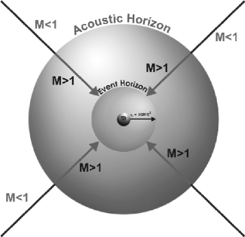
Figure 1: Spherically symmetric transonic black hole accretion with acoustic horizon.

X.2 Mono-transonic Spherical Accretion

Investigation of accretion processes onto celestial objects was initiated by Hoyle & Lyttleton (1939) by computing the rate at which pressure-less matter would be captured by a moving star. Subsequently, theory of stationary, spherically symmetric and transonic hydrodynamic accretion of adiabatic fluid onto a gravitating astrophysical object at rest was formulated in a seminal paper by Bondi (1952) using purely Newtonian potential and by including the pressure effect of the accreting material. Later on, Michel (1972) discussed fully general relativistic polytropic accretion on to a Schwarzschild black hole by formulating the governing equations for steady spherical flow of perfect fluid in Schwarzschild metric. Following Michel’s relativistic generalization of Bondi’s treatment, Begelman (1978) and Moncrief (1980) discussed some aspects of the sonic points of the flow for such an accretion. Spherical accretion and wind in general relativity have also been considered using equations of state other than the polytropic one and by incorporating various radiative processes (Shapiro 1973, 1973a; Blumenthal & Mathews 1976; Brinkmann 1980). Malec (1999) provided the solution for general relativistic spherical accretion with and without back reaction, and showed that relativistic effects enhance mass accretion when back reaction is neglected. The exact values of dynamical and thermodynamic accretion variables on the sonic surface, and at extreme close vicinity of the black hole event horizons, have recently been calculated using complete general relativistic (Das 2002) as well as pseudo general relativistic (Das & Sarkar 2001) treatments.

Figure 1 pictorially illustrates the generation of the acoustic horizon for spherical transonic accretion. Let us assume that an isolated black hole at rest accretes matter. The black hole (denoted by B in the figure) is assumed to be of Schwarzschild type, and is embedded by an gravitational event horizon of radius $2GM_{BH}/c^{2}$. Infalling matter is assumed not to possess any intrinsic angular momentum, and hence, falls freely on to the black hole radially. Such an accreting system possesses spherical symmetry. Far away from the black hole the dynamical fluid velocity is negligible and hence the matter is subsonic, which is demonstrated in the figure by M $<$ 1. In course of its motion toward the event horizon, accreting material acquires sufficiently large dynamical velocity due to the black hole’s strong gravitational attraction. Consequently, at a certain radial distance, the Mach number becomes unity. The particular value of $r$, for which M=1, is referred as the transonic point or the sonic point, and is denoted by $r_{h}$, as mentioned in the above section. For $r<r_{h}$, matter becomes supersonic and any acoustic signal created in that region is bound to be dragged toward the black hole, and can not escape to the region $r>r_{h}$. In other words, any co-moving observer from $r{\leq}r_{h}$ can not communicate with another observer at $r>r_{h}$ by sending any signal traveling with velocity $v_{\rm signal}{\leq}c_{s}$.Hence the spherical surface through $r_{h}$ is actually an acoustic horizon for stationary configuration, which is generated when accreting fluid makes a transition from subsonic (M $<$ 1) to the supersonic (M $>$ 1) state. In subsequent sections, we will demonstrate how one can determine the location of $r_{h}$ and how the surface gravity and the analogue Hawking temperature corresponding to such $r_{h}$ can be computed. Note, however, that for spherically symmetric accretion, only one acoustic horizon may form for a given set of initial boundary configuration characterizing the stationary configuration. For matter accreting with non-zero intrinsic angular momentum, multiple acoustic horizons can be obtained. Details of such configurations will be discussed in subsequent sections.

It is perhaps relevant to mention that spherical black hole accretion can allow standing shock formation. Perturbations of various kinds may produce discontinuities in an astrophysical fluid flow. By discontinuity at a surface in a fluid flow we understand any discontinuous change of a dynamical or a thermodynamic quantity across the surface. The corresponding surface is called a surface of discontinuity. Certain boundary conditions must be satisfied across such surfaces and according to these conditions, surfaces of discontinuities are classified into various categories. The most important such discontinuities are shock waves or shocks.

While the possibility of the formation of a standing spherical shock around compact objects was first conceived long ago (Bisnovatyi-Kogan, Zel‘Dovich, & Sunyaev 1971), most of the works on shock formation in spherical accretion share more or less the same philosophy that one should incorporate shock formation to increase the efficiency of directed radial infall in order to explain the high luminosity of AGNs and QSOs and to model their broad band spectrum (Jones & Ellison 1991). Considerable work has been done in this direction where several authors have investigated the formation and dynamics of standing shock in spherical accretion (Mészáros & Ostriker 1983; Protheros & Kazanas 1983; Chang & Osttriker 1985; Kazanas & Ellision 1986; Babul, Ostriker & Mészáros 1989; Park 1990, 1990a).

Study of spherically symmetric black hole accretion leads to the discovery of related interesting problems like entropic-acoustic or various other instabilities in spherical accretion (Foglizzo & Tagger 2000; Blondin & Ellison 2001; Lai & Goldreich 2000; Foglizzo 2001; Kovalenko & Eremin 1998), the realizability and the stability properties of Bondi solutions (Ray & Bhattacharjee 2002), production of high energy cosmic rays from AGNs (Protheroe & Szabo 1992), study of the hadronic model of AGNs (Blondin & Konigl 1987; Contopoulos & Kazanas 1995), high energetic emission from relativistic particles in our galactic centre (Markoff, Melia & Sarcevic 1999), explanation of high lithium abundances in the late-type, low-mass companions of the soft X-ray transient, (Guessoum & Kazanas 1999), study of accretion powered spherical winds emanating from galactic and extra galactic black hole environments (Das 2001).

X.3 Breaking the Spherical Symmetry: Accretion Disc

X.3.1 A General Overview

In sixties, possible disc-like structures around one of the binary components were found (Kraft, 1963) and some tentative suggestions that matter should accrete in the form of discs were put forward (Pendergest & Burbidge 1968; Lynden-Bell 1969). Meanwhile, it was understood that for spherically symmetric accretion discussed above, the (radial) infall velocity is very high, hence emission from such a rapidly falling matter was not found to be strong enough to explain the high luminosity of Quasars and AGNs. Introducing the idea of magnetic dissipation, efforts were made to improve the luminosity (Shvartsman 1971, 1971a; Shapiro 1973, 1973a).

Theoretically, accretion discs around black holes were first envisaged to occur within a binary stellar system where one of the components is compact object (i.e., white dwarfs, neutron stars or a black hole) and the secondary would feed matter onto the primary either through an wind or through Roche lobe overflow. In either case, the accreted matter would clearly possesses substantial intrinsic angular momentum with respect to the compact object (a black hole, for our discussion). A flow with that much angular momentum will have much smaller infall velocity and much higher density compared to the spherical accretion. The infall time being higher, viscosity within the fluid, presumably produced by turbulence or magnetic field, would have time to dissipate angular momentum (except in regions close to the black holes, since large radial velocity close the event horizon leads to the typical value of dynamical time scale much smaller compared to the viscous time scale) and energy. As matter loses angular momentum, it sinks deeper into the gravitational potential well and radiate more efficiently. The flow encircles the compact accretor and forms a quasi-stationary disc like structure around the compact object and preferably in the orbital plane of it. Clear evidences for such accretion discs around white dwarfs in binaries was provided by analysis of Cataclysmic variable (Robinson 1976).

Accretion forming a Keplarian disc around a Schwarzschild black hole produces efficiency $\eta$ (the fraction of gravitational energy released) of the order of $\eta\sim 0.057$ and accretion onto a maximally rotating Kerr black hole is even more efficient, yielding $\eta\sim 0.42$. However, the actual efficiencies depends on quantities such as viscosity parameters and the cooling process inside the disc (see Wiita 1998 and references therein). This energy is released in the entire electromagnetic spectrum and the success of a disc model depends on its ability to describe the way this energy is distributed in various frequency band.

In case of binary systems, where one of the components is a compact object like white dwarfs, neutron star or a black hole, the companion is stripped off its matter due to the tidal effects. The stripped off matter, with angular momentum equal to that of the companion, gradually falls towards the central compact object as the angular momentum is removed by viscosity. As the flow possesses a considerable angular momentum to begin with, it is reasonable to assume that the disc will form and the viscosity would transport angular momentum from inner part of the disc radially to the outer part which allows matter to further fall onto the compact body. This situation could be described properly by standard thin accretion disc, which may be Keplarian in nature. On the other hand, in the case of active galaxies and quasars, the situation could be somewhat different. The supermassive ($M_{BH}\lower 2.15277pt\hbox{$\;\buildrel>\over{\sim}\;$}10^{6}M_{\odot}$) central black hole is immersed in the intergalactic matter. In absence of any binary companion, matter is supplied to the central black hole very intermittently, and the angular momentum of the accreting matter at the outer edge of the disc may be sub-Keplarian. This low angular momentum flow departs the disc from Keplarian in nature and a ‘thick disc’ is more appropriate to describe the behaviour instead of standard thin, Keplarian Shakura Sunyaev (Shakura & Sunyaev 1973) disc.

X.3.2 Thin Disc Model

In standard thin disc model (Shakura & Sunyaev 1973; Novikov & Thorne 1973), originally conceived to describe Roche lobe accretion in a binary system, the local height $H(r)$ of the disc is assumed to be small enough compared to the local radius of the disc $r$, i.e., the ‘thinness’ condition is dictated by the fact that $H(r)<<r$. Pressure is neglected so that the radial force balance equations dictates the specific angular momentum distribution to become Keplarian and the radial velocity is negligible compared to the azimuthal velocity ($v_{r}<<v_{\phi}$). Unlike the spherical accretion, temperature distribution is far below than virial. Under the above mentioned set of assumptions, radial equations of steady state disc structure could be decoupled from the vertical ones and could be solved independently. The complete solutions describing the steady state disc structure can be obtained by solving four relativistic conservation equations, namely; the conservation of rest mass, specific angular momentum, specific energy and vertical momentum balance condition. In addition, a viscosity law may be specified which may transport angular momentum outwards allowing matter to fall in. On the top of it, in standard thin disc model, the shear is approximated as proportional to the pressure of the disc with proportionality constant $\alpha$, $\alpha$ being the viscosity parameter having numerical value less than unity.

High uncertainty remains in investigating the exact nature of the viscosity inside a thin accretion disc (see Wiita 1998 and references therein). One of the major problems is to explain the origin of sufficiently large viscosity that seems to be present inside accretion discs in the binary system. Unfortunately, under nearly all astrophysically relevant circumstances, all of the well understood microscopic transverse momentum transport mechanism such as ionic, molecular and radiative viscosity are extremely small. Observations with direct relevance to the nature and strength of the macroscopic viscosity mechanism are very difficult to make; the only fairly direct observational evidence for the strength of disc viscosity comes from the dwarf novae system. For a black hole as compact accretor, such observational evidences is far from reality till date. Therefore advances in understanding the disc viscosity is largely based on theoretical analysis and numerical techniques. Usually accepted view is that the viscosity may be due to magnetic transport of angular momentum or due to small scale turbulent dissipation. Over the past several years an explanation of viscosity in terms of Velikhov-Chandrasekhar-Balbus-Hawley instability (linear magnetic instability) has been investigated; see, e.g., Balbus & Hawle 1998 for further details.

X.3.3 Thick Disc Model

The assumptions implying accretion discs are always thin can break down in the innermost region. Careful consideration of the effects of general relativity show that the flow must go supersonically through a cusp. For considerably high accretion rate, radiation emitted by the in-falling matter exerts a significant pressure on the gas. The radiation pressure inflates the disc, and make it geometrically thick ($H(r)\sim r$, at least for the inner $10-100r_{g}$), which is often otherwise known as ‘accretion torus’. This considerable amount of radiation pressure must be incorporated to find the dynamical structure of the disc and in determining the thermodynamical quantities inside the disc. Incorporation of the radiation pressure term in Euler equation dictates the angular momentum deviation from that of the Keplarian. The angular momentum distribution becomes super (sub) Keplarian if the pressure gradient is positive (negative).

Introducing a post-Newtonian (these ‘pseudo’ potentials are widely used to mimic the space time around the Schwarzschild or the Kerr metric very nicely, see section 14 for details) $\Phi=-\frac{GM_{BH}}{(r-2r_{g})}$ in lieu of the usual $\Phi_{Newtonian}=-\frac{GM_{BH}}{r}$ (where $r_{g}$ is the ‘gravitational’ radius), Paczyński and Wiita (1980) provided the first thick disc model which joins with the standard thin disc at large radius without any discontinuity. They pointed out several important features of these configuration. It has been shown that the structure of thick disc in inner region is nearly independent of the viscosity and efficiency of accretion drops dramatically. More sophisticated model of radiation supported thick disc including self-gravity of the disc with full general relativistic treatment was introduced later (Wiita 1982; Lanza 1992).

X.3.4 Further Developments

Despite having a couple of interesting features, standard thick accretion disc model suffers from some limitations for which its study fell from favour in the late ’80s. Firstly, the strong anisotropic nature of the emission properties of the disc has been a major disadvantage. Secondly, a non-accreting thick disc is found to be dynamically and globally unstable to non-axisymmetric perturbations. However, an ideal ‘classical thick disc’, if modified to incorporate high accretion rates involving both low angular momentum and considerable radial infall velocity self-consistently, may remain viable. Also, it had been realized that neither the Bondi (1952) flow nor the standard thin disc model could individually fit the bill completely. Accretion disc theorists were convinced about the necessity of having an intermediate model which could bridge the gap between purely spherical flow (Bondi type) and purely rotating flow (standard thin disc). Such modification could be accomplished by incorporating a self-consistent ‘advection’ term which could take care of finite radial velocity of accreting material (for the black hole candidates which may gradually approaches the velocity of light to satisfy the inner boundary condition on event horizon) along with its rotational velocity and generalized heating and cooling terms (Hoshi & Shibazaki 1977; Liang & Thompson 1980; Ichimaru 1977; Paczyński & Bisnobhatyi-Kogan 1981; Abramowicz & Zurek 1981; Muchotrzeb & Paczyński 1982; Muchotrzeb 1983; Fukue 1987; Abramowicz et al. 1988; Narayan & Yi 1994; Chakrabarti 1989, 1996).

X.4 Multi-transonic Accretion Disc

For certain values of the intrinsic angular momentum density of accreting material, the number of sonic point, unlike spherical accretion, may exceed one, and accretion is called ‘multi-transonic’. Study of such multi-transonicity was initiated by Abramowicz & Zurek (1981). Subsequently, multi-transonic accretion disc has been studied in a number of works (Fukue 1987; Chakrabarti 1990, 1996; Kafatos & Yang 1994; Yang & Kafatos 1995; Pariev 1996; Peitz & Appl 1997; Lasota & Abramowicz 1997; Lu, Yu, Yuan & Young 1997; Das 2004; Barai, Das & Wiita 2004; Abraham, Bilić & Das 2006; Das, Bilić & Dasgupta 2006). All the above works, except Barai, Das & Wiita 2004, usually deal with low angular momentum sub-Keplerian inviscid flow around a Schwarzschild black hole or a prograde flow around a Kerr black hole. Barai, Das & Wiita 2004 studied the retrograde flows as well and showed that a higher angular momentum (as high as Keplerian) retrograde flow can also produce multi-transonicity. Sub-Keplerian weakly rotating flows are exhibited in various physical situations, such as detached binary systems fed by accretion from OB stellar winds (Illarionov & Sunyaev 1975; Liang & Nolan 1984), semi-detached low-mass non-magnetic binaries (Bisikalo et al. 1998), and super-massive black holes fed by accretion from slowly rotating central stellar clusters (Illarionov 1988; Ho 1999 and references therein). Even for a standard Keplerian accretion disc, turbulence may produce such low angular momentum flow (see, e.g., Igumenshchev & Abramowicz 1999, and references therein).

X.5 Non-axisymmetric Accretion Disc

All the above mentioned works deals with ‘axisymmetric’ accretion, for which the orbital angular momentum of the entire disc plane remains aligned with the spin angular momentum of the compact object of our consideration. In a strongly coupled binary system (with a compact object as one of the components), accretion may experience a non-axisymmetric potential because the secondary donor star may exert non-axisymmetric tidal force on the accretion disc around the compact primary. In general, non-axisymmetric tilted disc may form if the accretion takes place out of the symmetry plane of the spinning compact object. Matter in such misaligned disc will experience a torque due to the general relativistic Lense-Thirring effect (Lense & Thirring 1918), leading to the precession of the inner disc plane. The differential precession with radius may cause stress and dissipative effects in the disc. If the torque remains strong enough compared to the internal viscous force, the inner region of the initially tilted disc may be forced to realigned itself with the spin angular momentum (symmetry plane) of the central accretor. This phenomena of partial re-alignment (out to a certain radial distance known as the ‘transition radius’ or the ‘alignment radius’) of the initially non-axisymmetric disc is known as the ‘Bardeen-Petterson effect’ (Bardeen & Petterson 1975). Such a transition radius can be obtained by balancing the precession and the inward drift or the viscous time scale.

Astrophysical accretion disc subjected to the Bardeen-Petterson effect becomes ‘twisted’ or ‘warped’. A large scale warp (twist) in the disc may modify the emergent spectrum and can influence the direction of the Quasar and micro-quasar jets emanating out from the inner region of the accretion disc (see, e.g., Maccarone 2002; Lu & Zhou 2005, and references therein).

Such a twisted disc may be thought as an ensemble of annuli of increasing radii, for which the variation of the direction of the orbital angular momentum occurs smoothly while crossing the alignment radius. System of equations describing such twisted disc have been formulated by several authors (see, e.g., Peterson 1977; Kumar 1988; Demianski & Ivanov 1997; and references therein), and the time scale required for a Kerr black hole to align its spin angular momentum with that of the initially misaligned accretion disc, has also been estimated (Scheuer & Feiler 1996). Numerical simulation using three dimensional Newtonian Smooth Particle Hydrodynamics (SPH) code (Nelson & Papaloizou 2000) as well as using fully general relativistic framework (Fragile & Anninos 2005) reveal the geometric structure of such discs.

We would, however, not like to explore the non-axisymmetric accretion further in this review. One of the main reasons for which is, as long as the acoustic horizon forms at a radial length scale smaller than that of the alignment radius (typically 100 $r_{g}$ - 1000 $r_{g}$, according to the original estimation of Bardeen & Petterson 1975), one need not implement the non-axisymmetric geometry to study the analogue effects.

X.6 Angular Momentum Supported Shock in Multi-transonic Accretion Disc

In an adiabatic flow of the Newtonian fluid, the shocks obey the following conditions (Landau & Lifshitz 1959)

$$\left[\left[{\rho}u\right]\right]=0,~{}\left[\left[p+{\rho}u^{2}\right]\right]=0,~{}\left[\left[\frac{u^{2}}{2}+h\right]\right]=0,$$ (45)

where $[[f]]$ denotes the discontinuity of $f$ across the surface of discontinuity, i.e.

$$\left[\left[f\right]\right]=f_{2}-f_{1},$$ (46)

with $f_{2}$ and $f_{1}$ being the boundary values of the quantity $f$ on the two sides of the surface. Such shock waves are quite often generated in various kinds of supersonic astrophysical flows having intrinsic angular momentum, resulting in a flow which becomes subsonic. This is because the repulsive centrifugal potential barrier experienced by such flows is sufficiently strong to brake the infalling motion and a stationary solution could be introduced only through a shock. Rotating, transonic astrophysical fluid flows are thus believed to be ‘prone’ to the shock formation phenomena.

One also expects that a shock formation in black-hole accretion discs might be a general phenomenon because shock waves in rotating astrophysical flows potentially provide an important and efficient mechanism for conversion of a significant amount of the gravitational energy into radiation by randomizing the directed infall motion of the accreting fluid. Hence, the shocks play an important role in governing the overall dynamical and radiative processes taking place in astrophysical fluids and plasma accreting onto black holes. The study of steady, standing, stationary shock waves produced in black hole accretion has acquired an important status, and a number of works studied the shock formation in black hole accretion discs (Fukue 1983; Hawley, Wilson & Smarr 1984; Ferrari et al. 1985; Sawada, Matsuda & Hachisu 1986; Spruit 1987; Chakrabarti 1989; Abramowicz & Chakrabarti 1990; Yang & Kafatos 1995; Chakrabarti 1996a; Lu, Yu, Yuan & Young 1997; Caditz & Tsuruta 1998; Tóth, Keppens & Botchev 1998; Das 2002; Takahashi, Rillet, Fukumura & Tsuruta 2002; Das, Pendharkar & Mitra 2003; Das 2004; Chakrabarti & Das 2004; Fukumura & Tsuruta 2004; Abraham, Bilić & Das 2006; Das, Bilić & Dasgupta 2006) For more details and for a more exhaustive list of references see, e.g., Chakrabarti 1996c and Das 2002.

Generally, the issue of the formation of steady, standing shock waves in black-hole accretion discs is addressed in two different ways. First, one can study the formation of Rankine-Hugoniot shock waves in a polytropic flow. Radiative cooling in this type of shock is quite inefficient. No energy is dissipated at the shock and the total specific energy of the accreting material is a shock-conserved quantity. Entropy is generated at the shock and the post-shock flow possesses a higher entropy accretion rate than its pre-shock counterpart. The flow changes its temperature permanently at the shock. Higher post-shock temperature puffs up the post-shock flow and a quasi-spherical, quasi-toroidal centrifugal pressure supported region is formed in the inner region of the accretion disc (see Das 2002, and references therein for further detail) which locally mimics a thick accretion flow.

Another class of the shock studies concentrates on the shock formation in isothermal black-hole accretion discs. The characteristic features of such shocks are quite different from the non-dissipative shocks discussed above. In isothermal shocks, the accretion flow dissipates a part of its energy and entropy at the shock surface to keep the post-shock temperature equal to its pre-shock value. This maintains the vertical thickness of the flow exactly the same just before and just after the shock is formed. Simultaneous jumps in energy and entropy join the pre-shock supersonic flow to its post-shock subsonic counterpart. For detailed discussion and references see, e.g., Das, Pendharkar & Mitra 2003, and Fukumura & Tsuruta 2004.

In section 13.5, we will construct and solve the equations governing the general relativistic Rankine-Hugoniot shock. The shocked accretion flow in general relativity and in post-Newtonian pseudo-Schwarzschild potentials will be discussed in the section 13.5 - 13.8 and 16.2 respectively.

XI Motivation to Study the Analogue Behaviour of Transonic Black Hole Accretion

Since the publication of the seminal paper by Bondi in 1952 (Bondi 1952), the transonic behaviour of accreting fluid onto compact astrophysical objects has been extensively studied in the astrophysics community, and the pioneering work by Unruh in 1981 (Unruh 1981), initiated a substantial number of works in the theory of analogue Hawking radiation with diverse fields of application stated in section 4 - 5. It is surprising that no attempt was made to bridge these two categories of research, astrophysical black hole accretion and the theory of analogue Hawking radiation, by providing a self-consistent study of analogue Hawking radiation for real astrophysical fluid flows, i.e., by establishing the fact that accreting black holes can be considered as a natural example of analogue system. Since both the theory of transonic astrophysical accretion and the theory of analogue Hawking radiation stem from almost exactly the same physics, the propagation of a transonic fluid with acoustic disturbances embedded into it, it is important to study analogue Hawking radiation for transonic accretion onto astrophysical black holes and to compute $T_{{AH}}$ for such accretion.

In the following sections, we will describe the details of the transonic accretion and will show how the accreting black hole system can be considered as a classical analogue system. We will first discuss general relativistic accretion of spherically symmetric (mono-transonic Bondi (1952) type accretion) and axisymmetric (multi-transonic disc accretion) flow. We will then introduce a number of post-Newtonian pseudo-Schwarzschild black hole potential, and will discuss black hole accretion under the influence of such modified potentials.

XII General Relativistic Spherical Accretion as an Analogue Gravity Model

In this section, we will demonstrate how one can construct and solve the equations governing the general relativistic, spherically symmetric, steady state accretion flow onto a Schwarzschild black hole. This section is largely based on Das 2004a.

Accretion flow described in this section is $\theta$ and $\phi$ symmetric and possesses only radial inflow velocity. In this section, we use the gravitational radius $r_{g}$ as $r_{g}={2G{M_{BH}}}/{c^{2}}$. The radial distances and velocities are scaled in units of $r_{g}$ and $c$ respectively and all other derived quantities are scaled accordingly; $G=c=M_{BH}=1$ is used. Accretion is governed by the radial part of the general relativistic time independent Euler and continuity equations in Schwarzschild metric. We will consider the stationary solutions. We assume the dynamical in-fall time scale to be short compared with any dissipation time scale during the accretion process.

XII.1 The Governing Equations

To describe the fluid, we use a polytropic equation of state (this is common in the theory of relativistic black hole accretion) of the form

$$p=K{\rho}^{\gamma},$$ (47)

where the polytropic index $\gamma$ (equal to the ratio of the two specific heats $c_{p}$ and $c_{v}$) of the accreting material is assumed to be constant throughout the fluid. A more realistic model of the flow would perhaps require a variable polytropic index having a functional dependence on the radial distance, i.e. $\gamma{\equiv}\gamma(r)$. However, we have performed the calculations for a sufficiently large range of $\gamma$ and we believe that all astrophysically relevant polytropic indices are covered in our analysis.

The constant $K$ in (47) may be related to the specific entropy of the fluid, provided there is no entropy generation during the flow. If in addition to (47) the Clapeyron equation for an ideal gas holds

$$p=\frac{\kappa_{B}}{{\mu}m_{p}}{\rho}T\,,$$ (48)

where $T$ is the locally measured temperature, $\mu$ the mean molecular weight, $m_{H}{\sim}m_{p}$ the mass of the hydrogen atom, then the specific entropy, i.e. the entropy per particle, is given by (Landau & Lifshitz 1959):

$$\sigma=\frac{1}{\gamma-1}\log K+\frac{\gamma}{\gamma-1}+{\rm constant},$$ (49)

where the constant depends on the chemical composition of the accreting material. Equation (49) confirms that $K$ in (47) is a measure of the specific entropy of the accreting matter.

The specific enthalpy of the accreting matter can now be defined as

$$h=\frac{\left(p+\epsilon\right)}{\rho}\,,$$ (50)

where the energy density $\epsilon$ includes the rest-mass density and the internal energy and may be written as

$$\epsilon=\rho+\frac{p}{\gamma-1}\,.$$ (51)

The adiabatic speed of sound is defined by

$$c_{s}^{2}=\frac{{\partial}p}{{\partial}{\epsilon}}{\Bigg{|}}_{\rm constant~{}entropy}\,.$$ (52)

From (51) we obtain

$$\frac{\partial{\rho}}{\partial{\epsilon}}=\left(\frac{\gamma-1-c_{s}^{2}}{\gamma-1}\right).$$ (53)

Combination of (52) and (47) gives

$$c_{s}^{2}=K{\rho}^{\gamma-1}{\gamma}\frac{\partial{\rho}}{\partial{\epsilon}}\,,$$ (54)

Using the above relations, one obtains the expression for the specific enthalpy

$$h=\frac{\gamma-1}{\gamma-1-c_{s}^{2}}\,.$$ (55)

The rest-mass density $\rho$, the pressure $p$, the temperature $T$ of the flow and the energy density $\epsilon$ may be expressed in terms of the speed of sound $c_{s}$ as

$$\rho=K^{-\frac{1}{\gamma-1}}\left(\frac{\gamma-1}{\gamma}\right)^{\frac{1}{\gamma-1}}\left(\frac{c_{s}^{2}}{\gamma-1-c_{s}^{2}}\right)^{\frac{1}{\gamma-1}},$$ (56)

$$p=K^{-\frac{1}{\gamma-1}}\left(\frac{\gamma-1}{\gamma}\right)^{\frac{\gamma}{\gamma-1}}\left(\frac{c_{s}^{2}}{\gamma-1-c_{s}^{2}}\right)^{\frac{\gamma}{\gamma-1}},$$ (57)

$$T=\frac{\kappa_{B}}{{\mu}m_{p}}\left(\frac{\gamma-1}{\gamma}\right)\left(\frac{c_{s}^{2}}{\gamma-1-c_{s}^{2}}\right),$$ (58)

$$\epsilon=K^{-\frac{1}{\gamma-1}}\left(\frac{\gamma-1}{\gamma}\right)^{\frac{1}{\gamma-1}}\left(\frac{c_{s}^{2}}{\gamma-1-c_{s}^{2}}\right)^{\frac{1}{\gamma-1}}\left[1+\frac{1}{\gamma}\left(\frac{c_{s}^{2}}{\gamma-1-c_{s}^{2}}\right)\right].$$ (59)

The conserved specific flow energy ${\cal E}$ (the relativistic analogue of Bernoulli’s constant) along each stream line reads ${\cal E}=hu_{t}$, (Anderson 1989) where $h$ and $u_{\mu}$ are the specific enthalpy and the four velocity, which can be re-cast in terms of the radial three velocity $u$ and the polytropic sound speed $c_{s}$ to obtain:

$${\cal E}=\left[\frac{\gamma-1}{\gamma-\left(1+c^{2}_{s}\right)}\right]\sqrt{\frac{1-1/r}{1-u^{2}}}$$ (60)

One concentrates on positive Bernoulli constant solutions. The mass accretion rate ${\dot{M}}$ may be obtained by integrating the continuity equation:

$${\dot{M}}=4{\pi}{\rho}ur^{2}\sqrt{\frac{r-1}{r\left(1-u^{2}\right)}}$$ (61)

where $\rho$ is the proper mass density.

We define the ‘entropy accretion rate’ ${\dot{\Xi}}$ as a quasi-constant multiple of the mass accretion rate in the following way:

$${\dot{\Xi}}=K^{\displaystyle{\frac{1}{1-\gamma}}}{\dot{M}}=4{\pi}{\rho}ur^{2}\sqrt{\frac{r-1}{r\left(1-u^{2}\right)}}\left[\frac{c^{2}_{s}\left(\gamma-1\right)}{\gamma-\left(1+c^{2}_{s}\right)}\right]$$ (62)

Note that, in the absence of creation or annihilation of matter, the mass accretion rate is a universal constant of motion, whereas the entropy accretion rate is not. As the expression for ${\dot{\Xi}}$ contains the quantity $K\equiv p/\rho^{\gamma}$, which measures the specific entropy of the flow, the entropy rate ${\dot{\Xi}}$ remains constant throughout the flow only if the entropy per particle remains locally unchanged. This latter condition may be violated if the accretion is accompanied by a shock. Thus, ${\dot{\Xi}}$ is a constant of motion for shock-free polytropic accretion and becomes discontinuous (increases) at the shock location, if a shock forms in the accretion. One can solve the two conservation equations for ${\cal E}$ and ${\dot{\Xi}}$ to obtain the complete accretion profile.

XII.2 Transonicity

Simultaneous solution of (60-62) provides the dynamical three velocity gradient at any radial distance $r$:

$$\frac{du}{dr}=\frac{u\left(1-u^{2}\right)\left[c^{2}_{s}\left(4r-3\right)-1\right]}{2r\left(r-1\right)\left(u^{2}-c^{2}_{s}\right)}=\frac{{\cal N}\left(r,u,c_{s}\right)}{{\cal D}\left(r,u,c_{s}\right)}$$ (63)

A real physical transonic flow must be smooth everywhere, except possibly at a shock. Hence, if the denominator ${{\cal D}\left(r,u,c_{s}\right)}$ of (63) vanishes at a point, the numerator ${{\cal N}\left(r,u,c_{s}\right)}$ must also vanish at that point to ensure the physical continuity of the flow. Borrowing the terminology from the dynamical systems theory (see, e.g., Jordan & Smith 2005), one therefore arrives at the critical point conditions by making ${{\cal D}\left(r,u,c_{s}\right)}$ and ${{\cal N}\left(r,u,c_{s}\right)}$ of (63) simultaneously equal to zero. We thus obtain the critical point conditions as:

$$u{\bf{{|_{(r=r_{c})}}}}=c_{s}{\bf{{|_{(r=r_{c})}}}}=\sqrt{\frac{1}{4r_{c}-3}},$$ (64)

$r_{c}$ being the location of the critical point or the so called ‘fixed point’ of the differential equation (63).

From (64), one easily obtains that $M_{c}$, the Mach number at the critical point, is exactly equal to unity. This ensures that the critical points are actually the sonic points, and thus, $r_{c}$ is actually the location of the acoustic event horizon. In this section, hereafter, we will thus use $r_{h}$ in place of $r_{c}$. Note, however, that the equivalence of the critical point with the sonic point (and thus with the acoustic horizon) is not a generic feature. Such an equivalence strongly depends on the flow geometry and the equation of state used. For spherically symmetric accretion (using any equation of state), or polytropic disc accretion where the expression for the disc height is taken to be constant (Abraham, Bilić & Das 2006), or isothermal disc accretion with variable disc height, such an equivalence holds good. For all other kind of disc accretion, critical points and the sonic points are not equivalent, and the acoustic horizon forms at the sonic points and not at the critical point. We will get back to this issue in greater detail in section 13.3.

Substitution of $u{\bf{{|_{(r=r_{h})}}}}$ and $c_{s}{\bf{{|_{(r=r_{h})}}}}$ into (60) for $r=r_{h}$ provides:

$$r_{h}^{3}+r_{h}^{2}\Gamma_{1}+r_{h}\Gamma_{2}+\Gamma_{3}=0$$ (65)

where

$$\Gamma_{1}=\left[\frac{2{\cal E}^{2}\left(2-3\gamma\right)+9\left(\gamma-1\right)}{4\left(\gamma-1\right)\left({\cal E}^{2}-1\right)}\right],$$

$$\Gamma_{2}=\left[\frac{{\cal E}^{2}\left(3\gamma-2\right)^{2}-27\left(\gamma-1\right)^{2}}{32\left({\cal E}^{2}-1\right)\left(\gamma-1\right)^{2}}\right],~{}\Gamma_{3}=\frac{27}{64\left({\cal E}^{2}-1\right)}.$$ (66)

Solution of (65) provides the location of the acoustic horizon in terms of only two accretion parameters $\{{\cal E},\gamma\}$, which is the two parameter input set to study the flow.

We now set the appropriate limits on $\left\{{\cal E},{\gamma}\right\}$to model the realistic situations encountered in astrophysics. As ${\cal E}$ is scaled in terms of the rest mass energy and includes the rest mass energy, ${\cal E}<1$ corresponds to the negative energy accretion state where radiative extraction of rest mass energy from the fluid is required. For such extraction to be made possible, the accreting fluid has to possess viscosity or other dissipative mechanisms, which may violate the Lorentzian invariance. On the other hand, although almost any ${\cal E}>1$ is mathematically allowed, large values of ${\cal E}$ represents flows starting from infinity with extremely high thermal energy (see section 13.4 for further detail), and ${\cal E}>2$ accretion represents enormously hot flow configurations at very large distance from the black hole, which are not properly conceivable in realistic astrophysical situations. Hence one sets $1{\lower 2.15277pt\hbox{$\;\buildrel<\over{\sim}\;$}}{\cal E}{\lower 2.15277pt\hbox{$\;\buildrel<\over{\sim}\;$}}2$. Now, $\gamma=1$ corresponds to isothermal accretion where accreting fluid remains optically thin. This is the physical lower limit for $\gamma$, and $\gamma<1$ is not realistic in accretion astrophysics. On the other hand, $\gamma>2$ is possible only for superdense matter with substantially large magnetic field (which requires the accreting material to be governed by general relativistic magneto-hydrodynamic equations, dealing with which is beyond the scope of this article) and direction dependent anisotropic pressure. One thus sets $1{\lower 2.15277pt\hbox{$\;\buildrel<\over{\sim}\;$}}\gamma{\lower 2.15277pt\hbox{$\;\buildrel<\over{\sim}\;$}}2$ as well, so $\left\{{\cal E},{\gamma}\right\}$has the boundaries $1{\lower 2.15277pt\hbox{$\;\buildrel<\over{\sim}\;$}}\{{\cal E},\gamma\}{\lower 2.15277pt\hbox{$\;\buildrel<\over{\sim}\;$}}2$. However, one should note that the most preferred values of $\gamma$ for realistic black hole accretion ranges from $4/3$ to $5/3$ (Frank, King & Raine 1992).

For any specific value of $\{{\cal E},\gamma\}$, (65) can be solved completely analytically by employing the Cardano-Tartaglia-del Ferro technique. One defines:

$$\Sigma_{1}=\frac{3\Gamma_{2}-\Gamma_{1}^{2}}{9},~{}\Sigma_{2}=\frac{9\Gamma_{1}\Gamma_{2}-27\Gamma_{3}-2\Gamma_{1}^{3}}{54},~{}\Psi=\Sigma_{1}^{3}+\Sigma_{2}^{2},~{}\Theta={\rm cos}^{-1}\left(\frac{\Sigma_{2}}{\sqrt{-\Sigma_{1}^{3}}}\right)$$

$$\Omega_{1}=\sqrt[3]{\Sigma_{2}+\sqrt{\Sigma_{2}^{2}+\Sigma_{1}^{3}}},~{}\Omega_{2}=\sqrt[3]{\Sigma_{2}-\sqrt{\Sigma_{2}^{2}+\Sigma_{1}^{3}}},~{}\Omega_{\pm}=\left(\Omega_{1}\pm\Omega_{2}\right)$$ (67)

so that the three roots for $r_{h}$ come out to be:

$${}^{1}\!r_{h}=-\frac{\Gamma_{1}}{3}+\Omega_{+},\quad\quad^{2}\!r_{h}=-\frac{\Gamma_{1}}{3}-\frac{1}{2}\left(\Omega_{+}-i\sqrt{3}\Omega_{-}\right),\quad\quad^{3}\!r_{h}=-\frac{\Gamma_{1}}{3}-\frac{1}{2}\left(\Omega_{-}-i\sqrt{3}\Omega_{-}\right)$$ (68)

However, note that not all ${}^{i}\!r_{h}\{i=1,2,3\}$ would be real for all $\left\{{\cal E},{\gamma}\right\}$. It is easy to show that if $\Psi>0$, only one root is real; if $\Psi=0$, all roots are real and at least two of them are identical; and if $\Psi<0$, all roots are real and distinct. Selection of the real physical ($r_{h}$ has to be greater than unity) roots requires a close look at the solution for $r_{h}$ for the astrophysically relevant range of $\left\{{\cal E},{\gamma}\right\}$. One finds that for the preferred range of $\left\{{\cal E},{\gamma}\right\}$, one always obtains $\Psi<0$. Hence the roots are always real and three real unequal roots can be computed as:

$${}^{1}\!{{r}}_{h}=2\sqrt{-\Sigma_{1}}{\rm cos}\left(\frac{\Theta}{3}\right)-\frac{\Gamma_{1}}{3},~{}^{2}\!{{r}}_{h}=2\sqrt{-\Sigma_{1}}{\rm cos}\left(\frac{\Theta+2\pi}{3}\right)-\frac{\Gamma_{1}}{3},$$

$${}^{3}\!{{r}}_{h}=2\sqrt{-\Sigma_{1}}{\rm cos}\left(\frac{\Theta+4\pi}{3}\right)-\frac{\Gamma_{1}}{3}$$ (69)

One finds that for all $1{\lower 2.15277pt\hbox{$\;\buildrel<\over{\sim}\;$}}$$\left\{{\cal E},{\gamma}\right\}$${\lower 2.15277pt\hbox{$\;\buildrel<\over{\sim}\;$}}2$, ${}^{2}\!{{r}}_{h}$ becomes negative. It is observed that $\{^{1}\!{{r}}_{h},^{3}\!{{r}}_{h}\}>1$ for most values of the astrophysically tuned $\left\{{\cal E},{\gamma}\right\}$. However, it is also found that ${}^{3}\!{{r}}_{h}$ does not allow steady physical flows to pass through it; either $u$, or $a_{s}$, or both, becomes superluminal before the flow reaches the actual event horizon, or the Mach number profile shows intrinsic fluctuations for $r<r_{h}$. This information is obtained by numerically integrating the complete flow profile passing through ${}^{3}\!{{r}}_{h}$. Hence it turns out that one needs to concentrate only on ${}^{1}\!{{r}}_{h}$ for realistic astrophysical black hole accretion. Both large ${\cal E}$ and large $\gamma$ enhance the thermal energy of the flow so that the accreting fluid acquires the large radial velocity to overcome $a_{s}$ only in the close vicinity of the black hole . Hence $r_{h}$ anti-correlates with $\left\{{\cal E},{\gamma}\right\}$.

The critical properties and stability of such acoustic horizons has recently been studied using a dynamical systems approach, see Mandal, Ray & Das 2007 for further details.

To obtain $(du/dr)$ and $(dc_{s}/dr)$ on the acoustic horizon, L’ Hospital’s rule is applied to (63) to have:

$$\left(\frac{du}{dr}\right)_{r=r_{h}}=\Phi_{12}-\Phi_{123},~{}\left(\frac{dc_{s}}{dr}\right)_{r=r_{h}}=\Phi_{4}\left(\frac{1}{\sqrt{4r_{h}-3}}+\frac{\Phi_{12}}{2}-\frac{\Phi_{123}}{2}\right)$$ (70)

where

$$\Phi_{12}=-\Phi_{2}/2\Phi_{1},~{}\Phi_{123}=\sqrt{\Phi_{2}^{2}-4\Phi_{1}\Phi_{3}}/2\Phi_{1},~{}\Phi_{1}=\frac{6r_{h}\left(r_{h}-1\right)}{\sqrt{4r_{h}-3}},~{}$$

$$\Phi_{2}=\frac{2}{4r_{h}-3}\left[4r_{h}\left(\gamma-1\right)-\left(3\gamma-2\right)\right],~{}$$

$$\Phi_{3}=\frac{8\left(r_{h}-1\right)}{\left(4r_{h}-3\right)^{\frac{5}{2}}}\left[r_{h}^{2}\left(\gamma-1\right)^{2}-r_{h}\left(10\gamma^{2}-19\gamma+9\right)+\left(6\gamma^{2}-11\gamma+3\right)\right],~{}$$

$$\Phi_{4}=\frac{2\left(2r_{h}-1\right)-\gamma\left(4r_{h}-3\right)}{4\left(r_{h}-1\right)}$$ (71)

XII.3 Analogue Temperature

For spherically symmetric general relativistic flow onto Schwarzschild black holes, one can evaluate the exact value of the Killing fields and Killing vectors to calculate the surface gravity for that geometry. The analogue Hawking temperature for such geometry comes out to be (Das 2004a)

$$T_{{AH}}=\frac{\hbar{c^{3}}}{4{\pi}{\kappa_{B}}GM_{BH}}\left[\frac{r_{h}^{1/2}\left(r_{h}-0.75\right)}{\left(r_{h}-1\right)^{3/2}}\right]\left|\frac{d}{dr}\left(c_{s}-u\right)\right|_{r=r_{h}},$$ (72)

where the values of $r_{h},(du/dr)_{h}$ and $(dc_{s}/dr)_{h}$ are obtained using the system of units and scaling used in this article.

It is evident from (72) that the exact value of $T_{AH}$ can be analytically calculated from the results obtained in the previous section. While (68) provides the location of the acoustic horizon ($r_{h}$), the value of $\left|\frac{d}{dr}\left(c-u\right)\right|_{r=r_{h}}$ is obtained from (70-71) as a function of ${\cal E}$ and $\gamma$, both of which are real, physical, measurable quantities. Note again, that, since $r_{h}$ and other quantities appearing in (72) are analytically calculated as a function of $\left\{{\cal E},{\gamma}\right\}$, (72) provides an exact analytical value of the general relativistic analogue Hawking temperature for all possible solutions of an spherically accreting astrophysical black hole system, something which has never been done in the literature before. If $\sqrt{4r_{h}-3}(1/2-1/\Phi_{4})(\Phi_{12}-\Phi_{123})>1$, one always obtains $(dc_{s}/dr<du/dr)_{h}$ from (70), which indicates the presence of the acoustic white holes at $r_{h}$. This inequality holds good for certain astrophysically relevant range of $\left\{{\cal E},{\gamma}\right\}$, thus acoustic white hole solutions are obtained for general relativistic, spherically symmetric black hole accretion, see Das 2004a for further detail.

For a particular value of $\left\{{\cal E},{\gamma}\right\}$, one can define the quantity $\tau$ to be the ratio of $T_{{AH}}$ and $T_{H}$ as:

$$\tau=\frac{T_{{AH}}}{T_{H}}.$$ (73)

It turns out that $\tau$ is independent of the mass of the black hole. Thus, by computing the value of $\tau$, we can compare the properties of the acoustic versus event horizon of an accreting black hole of any mass, starting from the primordial black hole to the super massive black holes at the dynamical centre of the galaxies.

For general relativistic spherical accretion, one finds that for certain range of $\left\{{\cal E},{\gamma}\right\}$, $T_{AH}$ exceeds (i.e., $\tau>1$) the value of $T_{H}$, hence the analogue Hawking temperature can be larger than the actual Hawking temperature, see Das 2004a for further details.

XIII Multi-transonic, Relativistic Accretion Disc as Analogue Gravity Model

XIII.1 The Stress Energy Tensor and Flow Dynamics

To provide a generalized description of axisymmetric fluid flow in strong gravity, one needs to solve the equations of motion for the fluid and the Einstein equations. The problem may be made tractable by assuming the accretion to be non-self gravitating so that the fluid dynamics may be dealt in a metric without back-reactions. To describe the flow, we use the Boyer-Lindquist co-ordinate (Boyer & Lindquist 1967), and an azimuthally Lorentz boosted orthonormal tetrad basis co-rotating with the accreting fluid. We define $\lambda$ to be the specific angular momentum of the flow. Since we are not interested in non-axisymmetric disc structure, we neglect any gravo-magneto-viscous non-alignment between $\lambda$ and black hole spin angular momentum. We consider the flow to be non-self-gravitating to exclude any back reaction on the metric. For this section, the gravitational radius $r_{g}$ is taken to be $GM_{BH}/c^{2}$.

The most general form of the energy momentum tensor for the compressible hydromagnetic astrophysical fluid (with a frozen in magnetic field) vulnerable to the shear, bulk viscosity and generalized energy exchange, may be expressed as (Novikov & Thorne 1973):

$${\Im}^{{\mu}{\nu}}={\Im}^{{\mu}{\nu}}_{M}+{\Im}^{{\mu}{\nu}}_{\bf B}$$ (74)

where ${\Im}^{{\mu}{\nu}}_{M}$ and ${\Im}^{{\mu}{\nu}}_{\bf B}$ are the fluid (matter) part and the Maxwellian (electromagnetic) part of the energy momentum tensor. ${\Im}^{{\mu}{\nu}}_{M}$ and ${\Im}^{{\mu}{\nu}}_{\bf B}$ may be expressed as:

$${\Im}^{{\mu}{\nu}}_{M}={\rho}v^{\mu}v^{\nu}+\left(p-\varsigma{\theta}\right)h^{\mu\nu}-2\eta{\sigma}^{\mu\nu}+{\rm q}^{\mu}v^{\nu}+v^{\mu}{{\rm q}^{\nu}},~{}{\Im}^{{\mu}{\nu}}_{\bf B}=\frac{1}{8\pi}\left({\rm B}^{2}v^{\mu}v^{\nu}+{\rm B}^{2}h^{\mu\nu}-2{\rm B}^{\mu}{\rm B}^{\nu}\right)$$ (75)

In the above expression, ${\rho}v^{\mu}v^{\nu}$ is the total mass energy density excluding the frozen-in magnetic field mass energy density as measured in the local rest frame of the baryons (local orthonormal frame, hereafter LRF, in which there is no net baryon flux in any direction). $ph^{\mu\nu}$ is the isotropic pressure for incompressible gas (had it been the case that $\theta$ would be zero). $\varsigma$ and $\eta$ are the co-efficient of bulk viscosity and of dynamic viscosity, respectively. Hence $-\varsigma{\theta}h^{\mu\nu}$ and $-2{\eta}{\sigma^{\mu\nu}}$ are the isotropic viscous stress and the viscous shear stress, respectively. ${\rm q}^{\mu}v^{\nu}+v^{\mu}{{\rm q}^{\nu}}$ is the energy and momentum flux, respectively, in LRF of the baryons. In the expression for ${\Im}^{{\mu}{\nu}}_{\bf B}$, ${\rm B}^{2}/8\pi$ in the first term represents the energy density, in the second term represents the magnetic pressure orthogonal to the magnetic field lines, and in third term magnetic tension along the field lines (all terms expressed in LRF), respectively.

Here, the electromagnetic field is described by the field tensor ${\cal F}^{{\mu}{\nu}}$ and it’s dual ${\cal F}^{{\ast}{\mu}{\nu}}$ (obtained from ${\cal F}^{{\mu}{\nu}}$ using Levi-Civita ‘flipping’ tensor ${\epsilon}^{{\mu}{\nu}{\alpha}{\beta}}$) satisfying the Maxwell equations through the vanishing of the four-divergence of ${\cal F}^{{\ast}{\mu}{\nu}}$. A complete description of flow behaviour could be obtained by taking the co-variant derivative of ${\Im}^{{\mu}{\nu}}$ and ${\rho}v^{\mu}$ to obtain the energy momentum conservation equations and the conservation of baryonic mass.

However, at this stage, the complete solution remains analytically untenable unless we are forced to adopt a number of simplified approximations. We would like to study the inviscid accretion of hydrodynamic fluid. Hence ${\Im}^{{\mu}{\nu}}$ may be described by the standard form of the energy momentum (stress-energy) tensor of a perfect perfect fluid:

$${\Im}^{{\mu}{\nu}}=\left(\epsilon+p\right)v_{\mu}v_{\nu}+pg_{{\mu}{\nu}},~{}{\rm or,}~{}{\bf T}=\left(\epsilon+p\right){\bf v}{\otimes}{\bf v}+p{\bf g}$$ (76)

Our calculation will thus be focused on the stationary axisymmetric solution of the energy momentum and baryon number conservation equations

$${{\Im}^{{\mu}{\nu}}}_{;\nu}=0;\;\;\;\;\;\left({\rho}{v^{\mu}}\right)_{;\mu}=0,$$ (77)

Specifying the metric to be stationary and axially symmetric, the two generators $\xi^{\mu}\equiv(\partial/\partial t)^{\mu}$ and $\phi^{\mu}\equiv(\partial/\partial\phi)^{\mu}$ of the temporal and axial isometry, respectively, are Killing vectors.

We consider the flow to be ‘advective’, i.e. to possess considerable radial three-velocity. The above-mentioned advective velocity, which we hereafter denote by $u$ and consider it to be confined on the equatorial plane, is essentially the three-velocity component perpendicular to the set of hypersurfaces $\{\Sigma_{v}\}$ defined by $v^{2}={\rm const}$, where $v$ is the magnitude of the 3-velocity. Each $\Sigma_{v}$ is timelike since its normal $\eta_{\mu}\propto\partial_{\mu}v^{2}$ is spacelike and may be normalized as $\eta^{\mu}\eta_{\mu}=1$.

We then define the specific angular momentum $\lambda$ and the angular velocity $\Omega$ as

$$\lambda=-\frac{v_{\phi}}{v_{t}};\;\;\;\;\;\Omega=\frac{v^{\phi}}{v^{t}}=-\frac{g_{t\phi}+\lambda{g}_{tt}}{{g_{\phi{\phi}}+\lambda{g}_{t{\phi}}}}\,,$$ (78)

The metric on the equatorial plane is given by (Novikov & Thorne 1973)

$$ds^{2}=g_{{\mu}{\nu}}dx^{\mu}dx^{\nu}=-\frac{r^{2}{\Delta}}{A}dt^{2}+\frac{A}{r^{2}}\left(d\phi-\omega{dt}\right)^{2}+\frac{r^{2}}{\Delta}dr^{2}+dz^{2},$$ (79)

where $\Delta=r^{2}-2r+a^{2},~{}A=r^{4}+r^{2}a^{2}+2ra^{2}$, and $\omega=2ar/A$, $a$ being the Kerr parameter related to the black-hole spin. The normalization condition $v^{\mu}{v}_{\mu}=-1$, together with the expressions for $\lambda$ and $\Omega$ in (78), provides the relationship between the advective velocity $u$ and the temporal component of the four velocity

$$v_{t}=\left[\frac{Ar^{2}\Delta}{\left(1-u^{2}\right)\left\{A^{2}-4\lambda arA+\lambda^{2}r^{2}\left(4a^{2}-r^{2}\Delta\right)\right\}}\right]^{1/2}.$$ (80)

In order to solve (77), we need to specify a realistic equation of state. In this work, we concentrate on polytropic accretion. However, polytropic accretion is not the only choice to describe the general relativistic axisymmetric black-hole accretion. Equations of state other than the adiabatic one, such as the isothermal equation (Yang & Kafatos 1995) or the two-temperature plasma (Manmoto 2000), have also been used to study the black-hole accretion flow.

Like spherical accretion, here also we assume the dynamical in-fall time scale to be short compared with any dissipation time scale during the accretion process. We have performed the calculations for a sufficiently large range of $\gamma$ and we believe that all astrophysically relevant polytropic indices are covered in our work.

XIII.2 Disc Geometry and the Conservation Equations

We assume that the disc has a radius-dependent local thickness $H(r)$, and its central plane coincides with the equatorial plane of the black hole. It is a standard practice in accretion disc theory (Matsumoto et. al. 1984; Paczy’nski 1987; Abramowicz, Czerny, Lasota & Szuszkiewicz 1988; Chen & Taam 1993; Kafatos & Yang 1994; Artemova, Björnsson & Novikov 1996; Narayan, Kato & Honma 1997; Wiita 1999; Hawley & Krolik 2001; Armitage, Reynolds & Chiang 2001) to use the vertically integrated model in describing the black-hole accretion discs where the equations of motion apply to the equatorial plane of the black hole, assuming the flow to be in hydrostatic equilibrium in the transverse direction. The assumption of hydrostatic equilibrium is justified for a thin flow because for such flows, the infall time scale is expected to exceed the local sound crossing time scale in the direction transverse to the flow. We follow the same procedure here. The thermodynamic flow variables are averaged over the disc height, i.e., a thermodynamic quantity $y$ used in our model is vertically integrated over the disc height and averaged as $\bar{y}=\int^{H}(r)_{0}(ydh)/\int^{H}(r)_{0}H(r)$.

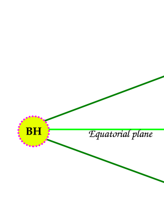
Figure 2: Height averaged thermodynamic quantities for disc accretion.

In figure 2, we schematically represent the above mentioned modelling. The yellow circular patch with BH written inside represents the black hole and the pink dashed boundary mimics the event horizon. The wedge shaped dark green lines represents the envelop of the accretion disc. The light green line centrally flanked by the two dark green disk boundaries, is the equatorial plane, on which all of the dynamical quantities (e.g., the advective velocity $u$) are assumed to be confined. Any thermodynamic quantity (e.g., the flow density) is averaged over the local disc height ${\bf h}(r)$ as shown in the figure.

We follow Abramowicz, Lanza & Percival (1997) to derive an expression for the disc height $H(r)$ in our flow geometry since the relevant equations in Abramowicz, Lanza & Percival (1997) are non-singular on the horizon and can accommodate both the axial and a quasi-spherical flow geometry. In the Newtonian framework, the disc height in vertical equilibrium is obtained from the $z$ component of the non-relativistic Euler equation where all the terms involving velocities and the higher powers of $\left({z}/{r}\right)$ are neglected. In the case of a general relativistic disc, the vertical pressure gradient in the comoving frame is compensated by the tidal gravitational field. We then obtain the disc height

$$H(r)=\sqrt{\frac{2}{\gamma+1}}r^{2}\left[\frac{(\gamma-1)c^{2}_{c}}{\{\gamma-(1+c^{2}_{s})\}\{\lambda^{2}v_{t}^{2}-a^{2}(v_{t}-1)\}}\right]^{\frac{1}{2}},$$ (81)

which, by making use of (80), may be be expressed in terms of the advective velocity $u$.

The temporal component of the energy momentum tensor conservation equation leads to the constancy along each streamline of the flow specific energy ${\cal E}$ (${\cal E}=hv_{t}$), and hence from (80) and (55) it follows that:

$${\cal E}=\left[\frac{(\gamma-1)}{\gamma-(1+c^{2}_{s})}\right]\sqrt{\left(\frac{1}{1-u^{2}}\right)\left[\frac{Ar^{2}\Delta}{A^{2}-4\lambda arA+\lambda^{2}r^{2}(4a^{2}-r^{2}\Delta)}\right]}\,.$$ (82)

The rest-mass accretion rate ${\dot{M}}$ is obtained by integrating the relativistic continuity equation (77). One finds

$${\dot{M}}=4{\pi}{\Delta}^{\frac{1}{2}}H{\rho}\frac{u}{\sqrt{1-u^{2}}}\,,$$ (83)

Here, we adopt the sign convention that a positive $u$ corresponds to accretion. The entropy accretion rate ${\dot{\Xi}}$ can be expressed as:

$${\dot{\Xi}}=\left(\frac{1}{\gamma}\right)^{\left(\frac{1}{\gamma-1}\right)}4\pi\Delta^{\frac{1}{2}}c_{s}^{\left(\frac{2}{\gamma-1}\right)}\frac{u}{\sqrt{1-u^{2}}}\left[\frac{(\gamma-1)}{\gamma-(1+c^{2}_{s})}\right]^{\left(\frac{1}{\gamma-1}\right)}H(r)$$ (84)

One can solve the conservation equations for ${\cal E},{\dot{M}}$ and ${\dot{\Xi}}$ to obtain the complete accretion profile.

XIII.3 Transonicity

The gradient of the acoustic velocity can be computed by differentiating (84) and can be obtained as:

$$\frac{dc_{s}}{dr}=\frac{c_{s}\left(\gamma-1-c_{s}^{2}\right)}{1+\gamma}\left[\frac{\chi{\psi_{a}}}{4}-\frac{2}{r}-\frac{1}{2u}\left(\frac{2+u{\psi_{a}}}{1-u^{2}}\right)\frac{du}{dr}\right]$$ (85)

The dynamical velocity gradient can then be calculated by differentiating (83) with the help of (85) as:

$$\frac{du}{dr}=\frac{\displaystyle\frac{2c_{s}^{2}}{\left(\gamma+1\right)}\left[\frac{r-1}{\Delta}+\frac{2}{r}-\frac{v_{t}\sigma\chi}{4\psi}\right]-\frac{\chi}{2}}{\displaystyle{\frac{u}{\left(1-u^{2}\right)}-\frac{2c_{s}^{2}}{\left(\gamma+1\right)\left(1-u^{2}\right)u}\left[1-\frac{u^{2}v_{t}\sigma}{2\psi}\right]}},$$ (86)

where

$$\psi=\lambda^{2}{v_{t}^{2}}-a^{2}\left(v_{t}-1\right),~{}\psi_{a}=\left(1-\frac{a^{2}}{\psi}\right),~{}\sigma=2\lambda^{2}v_{t}-a^{2},~{}$$

$$\chi=\frac{1}{\Delta}\frac{d\Delta}{dr}+\frac{\lambda}{\left(1-\Omega\lambda\right)}\frac{d\Omega}{dr}-\frac{\displaystyle{\left(\frac{dg_{\phi\phi}}{dr}+\lambda\frac{dg_{t\phi}}{dr}\right)}}{\left(g_{\phi\phi}+\lambda g_{t\phi}\right)}.$$ (87)

The critical point conditions can be obtained as:

$${c_{s}}_{\bf{{|_{(r=r_{c})}}}}={\left[\frac{u^{2}\left(\gamma+1\right)\psi}{2\psi-u^{2}v_{t}\sigma}\right]^{1/2}_{\bf{{|_{(r=r_{c})}}}}},~{}~{}u{\bf{{|_{(r=r_{c})}}}}={\left[\frac{\chi\Delta r}{2r\left(r-1\right)+4\Delta}\right]^{1/2}_{\rm r=r_{c}}},$$ (88)

For any value of $\left[{\cal E},\lambda,\gamma,a\right]$, substitution of the values of $u{\bf{{|_{(r=r_{c})}}}}$ and $c_{s}{|}_{\rm r=r_{c}}$ in terms of $r_{c}$ in the expression for ${\cal E}$ (82), provides a polynomial in $r_{c}$, the solution of which determines the location of the critical point(s) $r_{c}$.

It is obvious from (88) that, unlike relativistic spherical accretion, $u_{\bf{{|_{(r=r_{c})}}}}{\neq}{c_{s}}_{\rm r=r_{c}}$, and hence the Mach number at the critical point is not equal to unity in general. This phenomena can more explicitly be demonstrated for $a=0$, i.e., for relativistic disc accretion in the Schwarzschild metric.

For Schwarzschild black hole, one can calculate the Mach number of the flow at the critical point as (Das, Bilić & Dasgupta 2006)

$$M_{c}=\sqrt{\left({\frac{2}{\gamma+1}}\right)\frac{{f_{1}}(r_{c},\lambda)}{{{f_{1}}(r_{c},\lambda)}+{{f_{2}}(r_{c},\lambda)}}}\,.$$ (89)

where

$${f_{1}}(r_{c},\lambda)=\frac{3r_{c}^{3}-2\lambda^{2}r_{c}+3{\lambda^{2}}}{r_{c}^{4}-\lambda^{2}r_{c}(r_{c}-2)},~{}{f_{2}}(r_{c},\lambda)=\frac{2r_{c}-3}{r_{c}(r_{c}-2)}-\frac{2r_{c}^{3}-\lambda^{2}r_{c}+\lambda^{2}}{r_{c}^{4}-\lambda^{2}r_{c}(r_{c}-2)}$$ (90)

Clearly, $M_{c}$ is generally not equal to unity, and for $\gamma\geq 1$, is always less than one.

Hence we distinguish a sonic point from a critical point. In the literature on transonic black-hole accretion discs, the concepts of critical and sonic points are often made synonymous by defining an ‘effective’ sound speed leading to the ‘effective’ Mach number (for further details, see, eg. Matsumoto et. al. 1984, Chakrabarti 1989). Such definitions were proposed as effects of a specific disc geometry. We, however, prefer to maintain the usual definition of the Mach number for two reasons.

First, in the existing literature on transonic disc accretion, the Mach number at the critical point turns out to be a function of $\gamma$ only, and hence $M_{c}$ remains constant if $\gamma$ is constant. For example, using the Paczyński and Wiita (1980) pseudo-Schwarzschild potential to describe the adiabatic accretion phenomena leads to (see section 16.1.1 for the derivation and for further details)

$$M_{c}=\sqrt{\frac{2}{\gamma+1}}\,.$$ (91)

The above expression does not depend on the location of the critical point and depends only on the value of the adiabatic index chosen to describe the flow. Note that for isothermal accretion $\gamma=1$ and hence the sonic points and the critical points are equivalent (since $M_{c}=1$), see (169) in section 16.1.2 for further details.

However, the quantity $M_{c}$ in Eq. (89) as well as in (88) is clearly a function of $r_{c}$, and hence, generally, it takes different values for different $r_{c}$ for transonic accretion. The difference between the radii of the critical point and the sonic point may be quite significant. One defines the radial difference of the critical and the sonic point (where the Mach number is exactly equal to unity) as

$${\Delta}r_{c}^{s}=|r_{s}-r_{c}|.$$ (92)

The quantity ${\Delta}r_{c}^{s}$ may be a complicated function of $\left[{\cal E},\lambda,\gamma,a\right]$, the form of which can not be expressed analytically. The radius $r_{s}$ in Eq. (92) is the radius of the sonic point corresponding to the same $\left[{\cal E},\lambda,\gamma,a\right]$for which the radius of the critical point $r_{c}$ is evaluated. Note, however, that since $r_{s}$ is calculated by integrating the flow from $r_{c}$, ${\Delta}r_{c}^{s}$ is defined only for saddle-type critical points (see subsequent paragraphs for further detail). This is because, a physically acceptable transonic solution can be constructed only through a saddle-type critical point. One can then show that ${\Delta}r_{c}^{s}$ can be as large as $10^{2}$ $r_{g}$ or even more (for further details, see Das, Bilić & Dasgupta 2006).

The second and perhaps the more important reason for keeping $r_{c}$ and $r_{s}$ distinct is the following. In addition to studying the dynamics of general relativistic transonic black-hole accretion, we are also interested in studying the analogue Hawking effects for such accretion flow. We need to identify the location of the acoustic horizon as a radial distance at which the Mach equals to one, hence, a sonic point, and not a critical point will be of our particular interest. To this end, we first calculate the critical point $r_{c}$ for a particular $\left[{\cal E},\lambda,\gamma,a\right]$following the procedure discussed above, and then we compute the location of the sonic point (the radial distance where the Mach number exactly equals to unity) by integrating the flow equations starting from the critical points. The dynamical and the acoustic velocity, as well as their space derivatives, at the sonic point, are then evaluated. The details of this procedure for the Schwarzschild metric are provided in Das, Bilić & Dasgupta 2006.

Furthermore, the definition of the acoustic metric in terms of the sound speed does not seem to be mathematically consistent with the idea of an ‘effective’ sound speed, irrespective of whether one deals with the Newtonian, post Newtonian, or a relativistic description of the accretion disc. Hence, we do not adopt the idea of identifying critical a point with a sonic point. However, for saddle-type critical points, $r_{c}$ and $r_{s}$ should always have one-to-one correspondence, in the sense that every critical point that allows a steady solution to pass through it is accompanied by a sonic point, generally at a different radial distance $r$.

It is worth emphasizing that the distinction between critical and sonic points is a direct manifestation of the non-trivial functional dependence of the disc thickness on the fluid velocity, the sound speed and the radial distance. In the simplest idealized case when the disc thickness is assumed to be constant, one would expect no distinction between critical and sonic points. In this case, as has been demonstrated for a thin disc accretion onto the Kerr black hole (Abraham, Bilić & Das 2006), the quantity $\Delta r_{c}^{s}$ vanishes identically for any astrophysically relevant value of $\left[{\cal E},\lambda,\gamma,a\right]$. Hereafter, we will use $r_{h}$ to denote the sonic point $r_{s}$, since a sonic point is actually the location of the acoustic horizon.

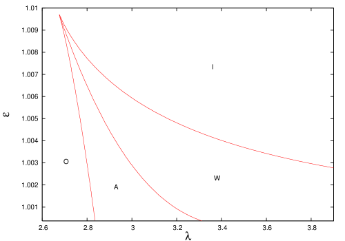
Figure 3: Parameter space for general relativistic multi-transonic accretion and wind in Kerr geometry, see text for detail. This figure is reproduced from Goswami, Khan, Ray & Das 2007.

XIII.4 Multi-transonic Behaviour

Unlike spherical accretion, one finds three (at most) critical points for relativistic disc accretion for some values of $\left[{\cal E},\lambda,\gamma,a\right]$. In figure 3, we classify the $\left[{\cal E},\lambda\right]$ parameter space, for a fixed value of adiabatic index ($\gamma=4/3$) and the Kerr parameter ($a=0.3$), to show the formation of various kind of critical points. The regions marked by O and I correspond to the formation of a single critical point, and hence the mono-transonic disc accretion is produced for such region. In the region marked by I, the critical points are called ‘inner type’ critical points since these points are quite close to the event horizon, approximately in the range $2<r_{c}^{\rm in}{\leq}10$. In the region marked by O, the critical points are called ‘outer type’ critical points, because these points are located considerably far away from the black hole. Depending on the value of $\left[{\cal E},\lambda,\gamma,a\right]$, an outer critical point may be as far as $10^{4}r_{g}$, or more.

The outer type critical points for the mono-transonic region are formed, as is obvious from the figure, for weakly rotating flow. For low angular momentum, accretion flow contains less amount of rotational energy, thus most of the kinetic energy in utilized to increase the radial dynamical velocity $u$ at a faster rate, leading to a higher value of $d^{2}u/dr^{2}$. Under such circumstances, the dynamical velocity $u$ becomes large enough to overcome the acoustic velocity $c_{s}$ at a larger radial distance from the event horizon, leading to the generation of supersonic flow at a large value of $r$, which results the formation of the sonic point (and hence the corresponding critical point) far away from the black hole event horizon. On the contrary, the inner type critical points are formed, as is observed from the figure, for strongly rotating flow in general. Owing to the fact that such flow would posses a large amount of rotational energy, only a small fraction of the total specific energy of the flow will be spent to increase the radial dynamical velocity $u$. Hence for such flow, $u$ can overcome $c_{s}$ only at a very small distance (very close to the event horizon) where the intensity of the gravitational field becomes enormously large, producing a very high value of the linear kinetic energy of the flow (high $u$), over shedding the contribution to the total specific energy from all other sources. However, from the figure it is also observed that the inner type sonic points are formed also for moderately low values of the angular momentum as well (especially in the region close to the vertex of the wedge shaped zone marked by W). For such regions, the total conserved specific energy is quite high. In the asymptotic limit, the expression for the total specific energy is governed by the Newtonian mechanics and one can have:

$${\cal E}=\left(\frac{u^{2}}{2}\right)_{\rm linear}+\left(\frac{c_{s}^{2}}{\gamma-1}\right)_{\rm thermal}+\left(\frac{\lambda^{2}}{2r^{2}}\right)_{\rm rotational}+\left(\Phi\right)_{\rm gravitational}$$ (93)

where $\Phi$ is the gravitational potential energy in the asymptotic limit, see section 16.1.1 for further detail. From (93) it is obvious that at a considerably large distance from the black hole, the contribution to the total energy of the flow comes mainly (rather entirely) from the thermal energy. A high value of ${\cal E}$ (flow energy in excess to its rest mass energy) corresponds to a ‘hot’ flow starting from infinity. Hence the acoustic velocity corresponding to the ‘hot’ flow obeying such outer boundary condition would be quite large. For such accretion, flow has to travel a large distance subsonically and can acquire a supersonic dynamical velocity $u$ only at a very close proximity to the event horizon, where the gravitational pull would be enormously strong.

The $\left[{\cal E},\lambda\right]$ corresponding to the wedge shaped regions marked by A and W produces three critical points, among which the largest and the smallest values correspond to the X type (saddle type), the outer $r_{c}^{out}$ and the inner $r_{c}^{in}$, critical points respectively. The O type (centre type) middle critical point, $r_{c}^{mid}$, which is unphysical in the sense that no steady transonic solution passes through it, lies in between $r_{c}^{in}$ and $r_{c}^{out}$. The following discussion provides the methodology for finding out the nature (whether saddle/centre type) in brief, see Goswami, Khan, Ray & Das 2007 for further detail.

Eq. (86) could be recast as

$$\frac{du^{2}}{dr}={\frac{\frac{2}{\gamma+1}c_{s}^{2}\left[\frac{g^{\prime}_{1}}{g_{1}}-\frac{1}{g_{2}}\frac{\partial g_{2}}{\partial r}\right]-\frac{f^{\prime}}{f}}{\frac{1}{1-u^{2}}\left(1-\frac{2}{\gamma+1}\frac{c_{s}^{2}}{u^{2}}\right)+\frac{2}{\gamma+1}\frac{c_{s}^{2}}{g_{2}}\left(\frac{\partial g_{2}}{\partial u^{2}}\right)}}$$ (94)

$$\frac{du^{2}}{d{\bar{\tau}}}=\frac{2}{\gamma+1}c_{s}^{2}\left[\frac{g^{\prime}_{1}}{g_{1}}-\frac{1}{g_{2}}\frac{\partial g_{2}}{\partial r}\right]-\frac{f^{\prime}}{f}$$ (95)

with the primes representing full derivatives with respect to $r$, and $\bar{\tau}$ is an arbitrary mathematical parameter. Here,

$$f(r)=\frac{Ar^{2}\Delta}{A^{2}-4\lambda arA+\lambda^{2}r^{2}(4a^{2}-r^{2}\Delta)},~{}$$

$$g_{1}i(r)=\Delta r^{4},~{}g_{2}(r,u)=\frac{\lambda^{2}f}{1-u^{2}}-\frac{a^{2}f^{\frac{1}{2}}}{\sqrt{1-u^{2}}}+a^{2}$$ (96)

The critical conditions are obtained with the simultaneous vanishing of the right hand side, and the coefficient of ${d(u^{2})/dr}$ in the left hand side in (94). This will provide

$$\left|\frac{2c_{s}^{2}}{\gamma+1}\left[\frac{g_{1}^{\prime}}{g_{1}}-\frac{1}{g_{2}}\left(\frac{\partial{g_{2}}}{\partial{r}}\right)\right]-\frac{f^{\prime}}{f}\right|_{\rm r=r_{c}}=\left|\frac{1}{1-u^{2}}\left(1-\frac{2}{\gamma+1}\frac{c_{s}^{2}}{u^{2}}\right)+\frac{2}{\gamma+1}\frac{c_{s}^{2}}{g_{2}}\left(\frac{\partial{g_{2}}}{\partial{u^{2}}}\right)\right|_{\rm r=r_{c}}=0$$ (97)

as the two critical point conditions. Some simple algebraic manipulations will show that

$$u_{c}^{2}=\frac{f^{\prime}g_{1}}{f{g_{1}^{\prime}}}$$ (98)

following which $c_{s}^{2}|_{\rm r=r_{c}}$ can be rendered as a function of $r_{c}$ only, and further, by use of (82)., $r_{c}$, $c_{sc}^{2}$ and $u_{c}^{2}$ can all be fixed in terms of the constants of motion like $E$, $\gamma$, $\lambda$ and $a$. Having fixed the critical points it should now be necessary to study their nature in their phase portrait of $u^{2}$ versus $r$. To that end one applies a perturbation about the fixed point values, going as,

$$u^{2}=u^{2}|_{\rm r=r_{c}}+\delta{u^{2}},~{}c_{s}^{2}=c_{s}^{2}|_{\rm r=r_{c}}+\delta{c_{s}^{2}},~{}r=r_{c}+\delta{r}$$ (99)

in the parameterized set of autonomous first-order differential equations,

$$\frac{d({u^{2}})}{d{\bar{\tau}}}=\frac{2}{\gamma+1}c_{s}^{2}\left[\frac{g_{1}^{\prime}}{g_{1}}-\frac{1}{g_{2}}\left(\frac{\partial{g_{2}}}{\partial{r}}\right)\right]\frac{f^{\prime}}{f}$$ (100)

and

$$\frac{dr}{d{\bar{\tau}}}=\frac{1}{1-u^{2}}\left(1-\frac{2}{\gamma+1}\frac{c_{s}^{2}}{u^{2}}\right)+\frac{1}{\gamma+1}\frac{c_{s}^{2}}{g_{2}}\left(\frac{\partial{g_{2}}}{\partial{u^{2}}}\right)$$ (101)

with ${\bar{\tau}}$ being an arbitrary parameter. In the two equations above $\delta c_{s}^{2}$ can be closed in terms of $\delta u^{2}$ and $\delta r$ with the help of (85). Having done so, one could then make use of solutions of the form, $\delta r\sim\exp({\bar{\Omega}}\tau)$ and $\delta u^{2}\sim\exp({\bar{\Omega}}\tau)$, from which, ${\bar{\Omega}}$ would give the eigenvalues — growth rates of $\delta u^{2}$ and $\delta r$ in ${\bar{\tau}}$ space — of the stability matrix implied by (100-101). Detailed calculations will show the eigenvalues to be

$${\bar{\Omega}}^{2}=\left|{\bar{\beta}}^{4}c_{s}^{4}\chi_{1}^{2}+\xi_{1}\xi_{2}\right|_{\rm r=r_{c}}$$ (102)

where ${\bar{\beta}}^{2}=\frac{2}{\gamma+1}$ and $\chi_{1},\xi_{1}$ and $\xi_{2}$ can be expressed as polynomials of $r_{c}$ (see Goswami, Khan, Ray & Das 2007 for the explicit form of the polynomial), hence ${\bar{\Omega}}^{2}$ can be evaluated for any $\left[{\cal E},\lambda,\gamma,a\right]$once the value of the corresponding critical point $r_{c}$ is known. The structure of (102) immediately shows that the only admissible critical points in the conserved Kerr system will be either saddle points or centre type points. For a saddle point, ${\bar{\Omega}}^{2}>0$, while for a centre-type point, ${\bar{\Omega}}^{2}<0$.

For multi-transonic flow characterized by a specific set of $\left[{\cal E},\lambda,\gamma,a\right]$, one can obtain the value of ${\bar{\Omega}}^{2}$ to be positive for $r_{c}^{in}$ and $r_{c}^{out}$, showing that those critical points are of saddle type in nature. ${\bar{\Omega}}^{2}$ comes out to be negative for $r_{c}^{mid}$, confirming that the middle sonic point is of centre type and hence no transonic solution passes through it. One can also confirm that all mono-transonic flow (flow with a single critical point characterized by $\left[{\cal E},\lambda\right]$ used from the green tinted region, either I or O) corresponds to saddle type critical point.

However, there is a distinct difference between the multi-transonic flow characterized by $\left[{\cal E},\lambda\right]$ taken from the region marked by A, and the region marked by W. For region marked by A, the entropy accretion rate ${\dot{\Xi}}$ for flows passing through the inner critical point is greater than that of the outer critical point

$${\dot{\Xi}}\left(r_{c}^{in}\right)>{\dot{\Xi}}\left(r_{c}^{out}\right)$$ (103)

while for the region marked by W, the following relation holds

$${\dot{\Xi}}\left(r_{c}^{in}\right)<{\dot{\Xi}}\left(r_{c}^{out}\right)$$ (104)

The above two relations show that $\left[{\cal E},\lambda\right]$ region marked by ${\cal A}$ represents multi-transonic accretion, while $\left[{\cal E},\lambda\right]{\in}\left[{\cal E},\lambda\right]_{\bf W}$ corresponds to the mono-transonic accretion but multi-transonic wind. More details about such classification will be discussed in the following paragraphs.

There are other regions for $\left[{\cal E},\lambda\right]$ space for which either no critical points are formed, or two critical points are formed. These regions are not shown in the figure. However, none of these regions is of our interest. If no critical point is found, it is obvious that transonic accretion does not form for those set of $\left[{\cal E},\lambda\right]$. For two critical point region, one of the critical points are always of ‘O’ type, since according to the standard dynamical systems theory two successive critical points can not be of same type (both saddle, or both centre). Hence the solution which passes through the saddle type critical point would encompass the centre type critical point by forming a loop (see, e.g., Das, Bilić & Dasgupta 2006 for such loop formation in Schwarzschild metric) like structure and hence such solution would not be physically acceptable since that solution will form a closed loop and will not connect infinity to the event horizon.

XIII.5 Multi-transonic Flow Topology and Shock Formation

To obtain the dynamical velocity gradient at the critical point, we apply l’Hospital’s rule on (86). After some algebraic manipulations, the following quadratic equation is formed, which can be solved to obtain $(du/dr)_{\bf{{|_{(r=r_{c})}}}}$ (see Barai, Das & Wiita 2004 for further details):

$$\alpha\left(\frac{du}{dr}\right)_{\bf{{|_{(r=r_{c})}}}}^{2}+\beta\left(\frac{du}{dr}\right)_{\bf{{|_{(r=r_{c})}}}}+\zeta=0,$$ (105)

where the coefficients are:

$$\alpha=\frac{\left(1+u^{2}\right)}{\left(1-u^{2}\right)^{2}}-\frac{2\delta_{1}\delta_{5}}{\gamma+1},\quad\quad\beta=\frac{2\delta_{1}\delta_{6}}{\gamma+1}+\tau_{6},\quad\quad\zeta=-\tau_{5};$$

$$\delta_{1}=\frac{c_{s}^{2}\left(1-\delta_{2}\right)}{u\left(1-u^{2}\right)},\quad\quad\delta_{2}=\frac{u^{2}v_{t}\sigma}{2\psi},\quad\quad\delta_{3}=\frac{1}{v_{t}}+\frac{2\lambda^{2}}{\sigma}-\frac{\sigma}{\psi},\quad\quad\delta_{4}=\delta_{2}\left[\frac{2}{u}+\frac{uv_{t}\delta_{3}}{1-u^{2}}\right],$$

$$~{}\delta_{5}=\frac{3u^{2}-1}{u\left(1-u^{2}\right)}-\frac{\delta_{4}}{1-\delta_{2}}-\frac{u\left(\gamma-1-c_{s}^{2}\right)}{a_{s}^{2}\left(1-u^{2}\right)},\quad\quad\delta_{6}=\frac{\left(\gamma-1-c_{s}^{2}\right)\chi}{2c_{s}^{2}}+\frac{\delta_{2}\delta_{3}\chi v_{t}}{2\left(1-\delta_{2}\right)},$$

$$\tau_{1}=\frac{r-1}{\Delta}+\frac{2}{r}-\frac{\sigma v_{t}\chi}{4\psi},\quad\quad\tau_{2}=\frac{\left(4\lambda^{2}v_{t}-a^{2}\right)\psi-v_{t}\sigma^{2}}{\sigma\psi},$$

$$\tau_{3}=\frac{\sigma\tau_{2}\chi}{4\psi},\quad\quad\tau_{4}=\frac{1}{\Delta}-\frac{2\left(r-1\right)^{2}}{\Delta^{2}}-\frac{2}{r^{2}}-\frac{v_{t}\sigma}{4\psi}\frac{d\chi}{dr},$$

$$\tau_{5}=\frac{2}{\gamma+1}\left[c_{s}^{2}\tau_{4}-\left\{\left(\gamma-1-c_{s}^{2}\right)\tau_{1}+v_{t}c_{s}^{2}\tau_{3}\right\}\frac{\chi}{2}\right]-\frac{1}{2}\frac{d\chi}{dr},$$

$$\tau_{6}=\frac{2v_{t}u}{\left(\gamma+1\right)\left(1-u^{2}\right)}\left[\frac{\tau_{1}}{v_{t}}\left(\gamma-1-c_{s}^{2}\right)+c_{s}^{2}\tau_{3}\right].$$ (106)

Note that all the above quantities are evaluated at the critical point.

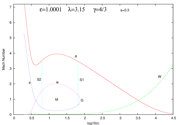
Figure 4: Solution topology for multi-transonic accretion in Kerr geometry for a specific set of $\left[{\cal E},\lambda,\gamma,a\right]$as shown in the figure. See text for detail.

Hence we compute the critical advective velocity gradient as

$$\left(\frac{du}{dr}\right)_{\rm r=r_{c}}=-\frac{\beta}{2\alpha}{\pm}\sqrt{\beta^{2}-4\alpha{\zeta}}$$ (107)

where the ‘+’ sign corresponds to the accretion solution and the ‘-’ sign corresponds to the wind solution, see the following discussion for further details. Similarly, the space gradient of the acoustic velocity $dc_{s}/dr$ and its value at the critical point can also be calculated.

The flow topology characterized by $\left[{\cal E},\lambda\right]$ corresponding to the I or O region (green tinted) is easy to obtain since the flow passes through only one saddle type critical point. Some of such representative topologies will be found in Das, Bilić & Dasgupta 2006 for the Schwarzschild metric. For Kerr metric, the flow profile would exactly be the same, only the numerical values for the critical/sonic point would be different, leading to the different values of $u$, $c_{s}$ and other corresponding accretion parameters at the same radial distance $r$. In this section we concentrate on multi-transonic flow topology, i.e., flow topology for $\left[{\cal E},\lambda\right]{\in}\left[{\cal E},\lambda\right]_{\bf A}$ or $\left[{\cal E},\lambda\right]{\in}\left[{\cal E},\lambda\right]_{\bf W}$. Figure 4 represents one such topology. While the local radial flow Mach number has been plotted along the $Y$ axis, the distance from the event horizon (scaled in the unit of $GM_{BH}/c^{2}$) in logarithmic unit has been plotted along the $X$ axis.

The solid red line marked by A corresponds to the transonic accretion passing through the outer critical point $r_{c}^{out}$. Using a specific set of $\left[{\cal E},\lambda,\gamma,a\right]$as shown in the figure, one first solve the equation for ${\cal E}$ at the critical point (using the critical point conditions as expressed in (88) to find out the corresponding three critical points, saddle type $r_{c}^{in}$ (4.279 $r_{g}$), centre type $r_{c}^{mid}$ (14.97 $r_{g}$) and saddle type $r_{c}^{out}$ (3315.01 $r_{g}$). The critical value of the advective velocity gradient at $r_{c}^{out}$ is then calculated using (105-107). Such $u_{\bf{{|_{(r=r_{c})}}}},{c_{s}}_{\bf{{|_{(r=r_{c})}}}}$ and $du/dr_{\bf{{|_{(r=r_{c})}}}}$ serve as the initial value condition for performing the numerical integration of the advective velocity gradient (86) using the fourth-order Runge-Kutta method. Such integration provides the outer sonic point $r_{s}^{out}$ ($r_{s}^{out}<r_{c}^{out}$), the local advective velocity, the polytropic sound speed, the Mach number, the fluid density, the disc height, the bulk temperature of the flow, and any other relevant dynamical and thermodynamic quantity characterizing the flow.

The dotted green line marked by W is obtained for the value of $du/dr_{\bf{{|_{(r=r_{c})}}}}$ corresponds to the ‘-’ sign in (107). Such a solution is called the corresponding ‘wind’ solution. The accretion and the wind solution intersects at the critical point (here, at $r_{c}^{out}$). This wind branch is just a mathematical counterpart of the accretion solution (velocity reversal symmetry of accretion), owing to the presence of the quadratic term of the dynamical velocity in the equation governing the energy momentum conservation. The term ‘wind solution’ has a historical origin. The solar wind solution first introduced by Parker (1965) has the same topology profile as that of the wind solution obtained in classical Newtonian Bondi accretion (Bondi 1952). Hence the name ‘wind solution’ has been adopted in a more general sense. The wind solution thus represents a hypothetical process, in which, instead of starting from infinity and heading towards the black hole, the flow generated near the black-hole event horizon would fly away from the black hole towards infinity.

The dashed blue line marked by ‘a’ and the dotted magenta line marked by ‘w’ are the respective accretion and the wind solutions passing through the inner critical point $r_{c}^{in}$ (the intersection of the accretion and the wind branch is the location of $r_{c}^{in}$). Such accretion and wind profile are obtained following exactly the same procedure as has been used to draw the accretion and wind topologies (red and green lines) passing through the outer critical point. Note, however, that the accretion solution through $r_{c}^{in}$ folds back onto the wind solution and the accretion-wind closed loop encompasses the middle sonic point, location of which is represented by $M$ in the figure. One should note that an ‘acceptable’ physical transonic solution must be globally consistent, i.e. it must connect the radial infinity $r{\rightarrow}\infty$ with the black-hole event horizon $r=2r_{g}$. . Hence, for multi-transonic accretion, there is no individual existence of physically acceptable accretion/wind solution passing through the inner critical (sonic) point, although such solution can be ‘clubbed’ with the accretion solution passing through $r_{c}^{out}$ through shock formation, see the following discussions for further details.

The set $\left[{\cal E},\lambda\right]_{\bf A}$ (or more generally $\left[{\cal E},\lambda,\gamma,a\right]_{\bf A}$) thus produces doubly degenerate accretion/wind solutions. Such two fold degeneracy may be removed by the entropy considerations since the entropy accretion rates ${\dot{\Xi}}$($r_{c}^{\rm in}$) and ${\dot{\Xi}}$($r_{c}^{\rm out}$) are generally not equal. For any $\left[{\cal E},\lambda,\gamma,a\right]{\in}\left[{\cal E},\lambda,\gamma,a\right]_{\bf A}$ we find that the entropy accretion rate ${\dot{\Xi}}$ evaluated for the complete accretion solution passing through the outer critical point is less than that of the rate evaluated for the incomplete accretion/wind solution passing through the inner critical point. Since the quantity ${\dot{\Xi}}$ is a measure of the specific entropy density of the flow, the solution passing through $r_{c}^{\rm out}$ will naturally tend to make a transition to its higher entropy counterpart, i.e. the incomplete accretion solution passing through $r_{c}^{\rm in}$. Hence, if there existed a mechanism for the accretion solution passing through the outer critical point (solid red line marked with A) to increase its entropy accretion rate by an amount

$${\Delta}{\dot{\Xi}}={\dot{\Xi}}(r_{c}^{\rm in})-{\dot{\Xi}}(r_{c}^{\rm out}),$$ (108)

there would be a transition to the incomplete accretion solution (dashed blue line marked with ‘a’) passing through the inner critical point. Such a transition would take place at a radial distance somewhere between the radius of the inner sonic point and the radius of the accretion/wind turning point (75.7 $r_{g}$) marked by G in the figure. In this way one would obtain a combined accretion solution connecting $r{\rightarrow}{\infty}$ with $r=2$ (the event horizon) which includes a part of the accretion solution passing through the inner critical, and hence the inner sonic point. One finds that for some specific values of $\left[{\cal E},\lambda,\gamma,a\right]_{\bf A}$, a standing Rankine-Hugoniot shock may accomplish this task. A supersonic accretion through the outer sonic point $r_{s}^{\rm out}$ (which in obtained by integrating the flow starting from the outer critical point $r_{c}^{out}$) can generate entropy through such a shock formation and can join the flow passing through the inner sonic point $r_{s}^{\rm in}$ (which in obtained by integrating the flow starting from the outer critical point $r_{c}^{in}$). Below we will carry on a detail discussion on such shock formation.

In this article, the basic equations governing the flow are the energy and baryon number conservation equations which contain no dissipative terms and the flow is assumed to be inviscid. Hence, the shock which may be produced in this way can only be of Rankine-Hugoniot type which conserves energy. The shock thickness must be very small in this case, otherwise non-dissipative flows may radiate energy through the upper and the lower boundaries because of the presence of strong temperature gradient in between the inner and outer boundaries of the shock thickness. In the presence of a shock the flow may have the following profile. A subsonic flow starting from infinity first becomes supersonic after crossing the outer sonic point and somewhere in between the outer sonic point and the inner sonic point the shock transition takes place and forces the solution to jump onto the corresponding subsonic branch. The hot and dense post-shock subsonic flow produced in this way becomes supersonic again after crossing the inner sonic point and ultimately dives supersonically into the black hole. A flow heading towards a neutron star can have the liberty of undergoing another shock transition after it crosses the inner sonic point , because the hard surface boundary condition of a neutron star by no means prevents the flow from hitting the star surface subsonically.

For the complete general relativistic accretion flow discussed in this article, the energy momentum tensor ${\Im}^{{\mu}{\nu}}$, the four-velocity $v_{\mu}$, and the speed of sound $c_{s}$ may have discontinuities at a hypersurface $\Sigma$ with its normal $\eta_{\mu}$. Using the energy momentum conservation and the continuity equation, one has

$$\left[\left[{\rho}v^{\mu}\right]\right]{\eta}_{\mu}=0,\left[\left[{\Im}^{\mu\nu}\right]\right]{\eta}_{\nu}=0.$$ (109)

For a perfect fluid, one can thus formulate the relativistic Rankine-Hugoniot conditions as

$$\left[\left[{\rho}u\Gamma_{u}\right]\right]=0,$$ (110)

$$\left[\left[{\Im}_{t\mu}{\eta}^{\mu}\right]\right]=\left[\left[(p+\epsilon)v_{t}u\Gamma_{u}\right]\right]=0,$$ (111)

$$\left[\left[{\Im}_{\mu\nu}{\eta}^{\mu}{\eta}^{\nu}\right]\right]=\left[\left[(p+\epsilon)u^{2}\Gamma_{u}^{2}+p\right]\right]=0,$$ (112)

where $\Gamma_{u}=1/\sqrt{1-u^{2}}$ is the Lorentz factor. The first two conditions (110) and (111) are trivially satisfied owing to the constancy of the specific energy and mass accretion rate. The constancy of mass accretion yields

$$\left[\left[K^{-\frac{1}{\gamma-1}}\left(\frac{\gamma-1}{\gamma}\right)^{\frac{1}{\gamma-1}}\left(\frac{c_{s}^{2}}{\gamma-1-c_{s}^{2}}\right)^{\frac{1}{\gamma-1}}\frac{u}{\sqrt{1-u^{2}}}H(r)\right]\right]=0.$$ (113)

The third Rankine-Hugoniot condition (112) may now be written as

$$\left[\left[K^{-\frac{1}{\gamma-1}}\left(\frac{\gamma-1}{\gamma}\right)^{\frac{\gamma}{\gamma-1}}\left(\frac{c_{s}^{2}}{\gamma-1-c_{s}^{2}}\right)^{\frac{\gamma}{\gamma-1}}\left\{\frac{u^{2}\left(\gamma-c_{s}^{2}\right)+c_{s}^{2}}{c_{s}^{2}\left(1-u^{2}\right)}\right\}\right]\right]=0.$$ (114)

Simultaneous solution of Eqs. (113) and (114) yields the ‘shock invariant’ quantity

$${\cal S}_{h}=c_{s}^{\frac{2\gamma+3}{\gamma-1}}\left(\gamma-1-c_{s}^{2}\right)^{\frac{3\gamma+1}{2\left(1-\gamma\right)}}u\left(1-u^{2}\right)^{-\frac{1}{2}}\left[\lambda^{2}v_{t}^{2}-a^{2}\left(v_{t}-1\right)\right]^{-\frac{1}{2}}\left[\frac{u^{2}\left(\gamma-c_{s}^{2}\right)+c_{s}^{2}}{c_{s}^{2}\left(1-u^{2}\right)}\right]$$ (115)

which changes continuously across the shock surface. We also define the shock strength ${\cal S}_{i}$ and the entropy enhancement $\Theta$ as the ratio of the pre-shock to post-shock Mach numbers (${\cal S}_{i}=M_{-}/M_{+}$), and as the ratio of the post-shock to pre-shock entropy accretion rates ($\Theta={\dot{\Xi}}_{+}/{\dot{\Xi}}_{-}$) of the flow, respectively. Hence, $\Theta={\dot{\Xi}}{(r_{c}^{in})}/{\dot{\Xi}}{r_{c}^{out}}$ for accretion and $\Theta={\dot{\Xi}}{(r_{c}^{out})}/{\dot{\Xi}}{r_{c}^{in}}$ for wind, respectively.

The shock location in multi-transonic accretion is found in the following way. Consider the multi-transonic flow topology as depicted in the Fig. 4. Integrating along the solution passing through the outer critical point, we calculate the shock invariant ${\cal S}_{h}$ in addition to $u$, $c_{s}$ and $M$. We also calculate ${\cal S}_{h}$ while integrating along the solution passing through the inner critical point, starting from the inner sonic point up to the point of inflexion G. We then determine the radial distance $r_{sh}$, where the numerical values of ${\cal S}_{h}$, obtained by integrating the two different sectors described above, are equal. Generally, for any value of $\left[{\cal E},\lambda,\gamma,a\right]$allowing shock formation, one finds two shock locations marked by S1 (the ‘outer’ shock, formed at 65.31$r_{g}$ – between the outer and the middle sonic points) and S2 (the ‘inner’ shock, formed at 6.31 $r_{g}$ – between the inner and the middle sonic points) in the figure. According to a standard local stability analysis (Yang & Kafatos 1995), for a multi-transonic accretion, one can show that only the shock formed between the middle and the outer sonic point is stable. The shock strength is different for the inner and for the outer shock. For the stable (outer) shock, the shock strength for the case shown in the figure is 5.586, hence it is a strong shock. Therefore, in the multi-transonic accretion with the topology shown in Fig. 4., the shock at S1 is stable and that at S2 is unstable. Hereafter, whenever we mention the shock location, we refer to the stable shock location only.

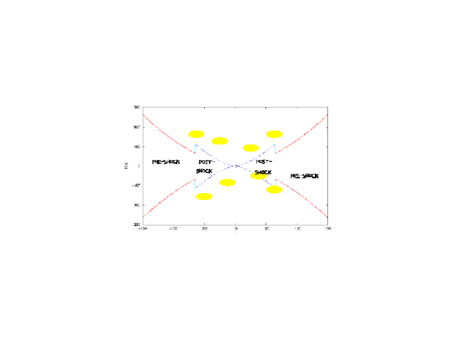
Figure 5: Pre- and post-shock disc geometry with thermally driven optically thick halo. See text for further detail.

XIII.6 Disc Geometry and Shock Generated Outflow

As a consequence of the shock formation in an accretion flow, the post-shock flow temperature will also increase abruptly. The post- to pre-shock temperature ratio $T_{+}/T_{-}$ is, in general, a sensitive function of $\left[{\cal E},\lambda,\gamma,a\right]$. In Fig. 5., we present the disc structure obtained by solving (81) for the combined shocked accretion flow. The point B represents the black-hole event horizon. The pre- and post-shock regions of the disc are clearly distinguished in the figure and show that the post-shock disc puffs up significantly. The pre-shock supersonic disc is shown by the red lines. The post-shock subsonic part of the disc is shown by dotted blue lines and the post-shock supersonic part (very close to the event horizon since $r_{c}^{in}=4.279r_{g}$) is shown by dotted magenta lines (not well resolved in the figure though). The bulk flow temperature will be increased in the post-shock region. Such an increased disc temperature may lead to a disc evaporation resulting in the formation of an optically thick halo, which are schematically shown using yellow coloured elliptic structures. Besides, a strong temperature enhancement may lead to the formation of thermally driven outflows. The generation of centrifugally driven and thermally driven outflows from black-hole accretion discs has been discussed in the post-Newtonian framework (Das & Chakrabarti 1999; Das, Rao & Vadawale 2003) The post-Newtonian approach may be extended to general relativity using the formalism presented here.

Owing to the very high radial component of the infall velocity of accreting material close to the black hole, the viscous time scale is much larger than the infall time scale. Hence, in the vicinity of the black hole, a rotating inflow entering the black hole will have an almost constant specific angular momentum for any moderate viscous stress. This angular momentum yields a very strong centrifugal force which increases much faster than the gravitational force. These two forces become comparable at some specific radial distance. At that point the matter starts piling up and produces a boundary layer supported by the centrifugal pressure, which may break the inflow to produce the shock. This actually happens not quite at the point where the gravitational and centrifugal forces become equal but slightly farther out owing to the thermal pressure. Still closer to the black hole, gravity inevitably wins and matter enters the horizon supersonically after passing through a sonic point. The formation of such a layer may be attributed to the shock formation in accreting fluid. The post-shock flow becomes hotter and denser, and for all practical purposes, behaves as the stellar atmosphere as far as the formation of outflows is concerned. A part of the hot and dense shock-compressed in-flowing material is then ‘squirted’ as an outflow from the post-shock region. Subsonic outflows originating from the puffed up hotter post-shock accretion disc (as shown in the figure) pass through the outflow sonic points and reach large distances as in a wind solution.

The generation of such shock-driven outflows is a reasonable assumption. A calculation describing the change of linear momentum of the accreting material in the direction perpendicular to the plane of the disc is beyond the scope of the disc model described in this article because the explicit variation of dynamical variables along the Z axis (axis perpendicular to the equatorial plane of the disc) cannot be treated analytically. The enormous post-shock thermal pressure is capable of providing a substantial amount of ‘hard push’ to the accreting material against the gravitational attraction of the black hole. This ‘thermal kick’ plays an important role in re-distributing the linear momentum of the inflow and generates a non-zero component along the Z direction. In other words, the thermal pressure at the post-shock region, being anisotropic in nature, may deflect a part of the inflow perpendicular to the equatorial plane of the disc. Recent work shows that (Moscibrodzka, Das & Czerny 2006) such shock-outflow model can be applied to successfully investigate the origin and dynamics of the strong X-ray flares emanating out from our galactic centre.

XIII.7 Multi-transonic Wind

The blue coloured wedge shaped region marked by W represents the $\left[{\cal E},\lambda,\gamma,a\right]$zone for which three critical points, the inner, the middle and the outer are also found. However, in contrast to $\left[{\cal E},\lambda,\gamma,a\right]{\in}\left[{\cal E},\lambda,\gamma,a\right]_{\bf A}$, the set $\left[{\cal E},\lambda,\gamma,a\right]{\in}\left[{\cal E},\lambda,\gamma,a\right]_{\bf W}$ yields solutions for which ${\dot{\Xi}}(r_{c}^{\rm in})$ is less than ${\dot{\Xi}}(r_{c}^{\rm out})$. Besides, the topological flow profile of these solutions is different. Here the closed loop-like structure is formed through the outer critical point. One such solution topology is presented in Fig. 6 for a specific set of $\left[{\cal E},\lambda,\gamma,a\right]$as shown in the figure. The same colour-scheme which has been used to denote various accretion and wind branches (through various critical points) of multi-transonic accretion (Fig. 4.), has been used here as well to manifest how the loop formation switches from flow through $r_{c}^{in}$ (multi-transonic accretion, Fig. 4.) to flow through $r_{c}^{out}$ (multi-transonic wind, Fig. 6.). This topology is interpreted in the following way. The flow (blue dashed line marked by ‘a’) passing through the inner critical point (3.456 $r_{g}$) is the complete mono-transonic accretion flow, and the dotted magenta line marked by ‘w’ is its corresponding wind solution. The solutions passing through the outer critical point (3307.318 $r_{g}$), represents the incomplete accretion (solid red line marked by ‘A’)/wind (dashed green line marked by ‘W’) solution. However, as ${\dot{\Xi}}(r_{c}^{in})$ turns out to be less than ${\dot{\Xi}}(r_{c}^{out})$, the wind solution through $r_{c}^{in}$ can make a shock transition to join its counter wind solution passing through $r_{c}^{out}$, and thereby increase the entropy accretion rate by the amount ${\Delta}{\dot{\Xi}}={\dot{\Xi}}(r_{c}^{out})-{\dot{\Xi}}(r_{c}^{in})$. Here the numerical values of ${\cal S}_{h}$ along the wind solution passing through the inner critical point are compared with the numerical values of ${\cal S}_{h}$ along the wind solution passing through the outer critical point, and the shock locations S1 and S2 for the wind are found accordingly. Here also, two theoretical shock locations are obtained, which are shown by dot dashed azure vertical lines marked by S1 (at 649.41 $r_{g}$) and S2 (at 6.42 $r_{g}$), out of which only one is stable. The shock strength corresponding to the stable outer shock can be calculated to be 20.24. Hence extremely strong shocks are formed for multi-transonic wind in general. A part of the region $\left[{\cal E},\lambda,\gamma,a\right]_{\bf W}$ thus corresponds to mono-transonic accretion solutions with multi-transonic wind solutions with a shock.

Besides $\gamma=4/3$ and $a=0.3$, for which Fig. 3. has been drawn, one can perform a similar classification for any astrophysically relevant value of $\gamma$ and $a$ as well. Some characteristic features of $\left[{\cal E},\lambda\right]$ would be changed as $\gamma$ is being varied. For example, if ${\cal E}_{\rm max}$ is the maximum value of the energy and if $\lambda_{\rm max}$ and $\lambda_{\rm min}$ are the maximum and the minimum values of the angular momentum, respectively, for $\left[{\cal E},\lambda\right]_{\bf A}$ for a fixed value of $\gamma$, then $\left[{\cal E}_{\rm max},\lambda_{\rm max},\lambda_{\rm min}\right]$ anti-correlates with $\gamma$. Hence, as the flow makes a transition from its ultra-relativistic to its purely non-relativistic limit, the area representing $\left[{\cal E},\lambda\right]_{\bf A}$ decreases.

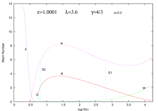
Figure 6: Solution topology for multi-transonic wind in Kerr geometry for a specific set of $\left[{\cal E},\lambda,\gamma,a\right]$as shown in the figure. See text for detail.

XIII.8 Dependence of Shock Location on Accretion Parameters

One finds that the shock location correlates with $\lambda$. This is obvious because the higher the flow angular momentum, the greater the rotational energy content of the flow. As a consequence, the strength of the centrifugal barrier which is responsible to break the incoming flow by forming a shock will be higher and the location of such a barrier will be farther away from the event horizon. However, the shock location anti-correlates with ${\cal E}$ and $\gamma$. This means that for the same ${\cal E}$ and $\lambda$, in the purely non-relativistic flow the shock will form closer to the black hole compared with the ultra-relativistic flow. Besides, we find that the shock strength ${\cal S}_{i}$ anti-correlates with the shock location $r_{sh}$, which indicates that the closer to the black hole the shock forms , the higher the strength ${\cal S}_{i}$ and the entropy enhancement ratio $\Theta$ are. The ultra-relativistic flows are supposed to produce the strongest shocks. The reason behind this is also easy to understand. The closer to the black hole the shock forms, the higher the available gravitational potential energy must be released, and the radial advective velocity required to have a more vigorous shock jump will be larger. Besides we note that as the flow gradually approaches its purely non-relativistic limit, the shock may form for lower and lower angular momentum, which indicates that for purely non-relativistic accretion, the shock formation may take place even for a quasi-spherical flow. However, it is important to mention that a shock formation will be allowed not for every $\left[{\cal E},\lambda,\gamma,a\right]{\in}\left[{\cal E},\lambda,\gamma,a\right]_{\bf A}$, Equation (115) will be satisfied only for a specific subset of $\left[{\cal E},\lambda,\gamma,a\right]_{\cal A}$, for which a steady, standing shock solution will be found.

XIII.9 Analogue Temperature

The surface gravity is defined according to (33). For axisymmetric accretion described in the above sections, one can calculate that (Abraham, Bilić & Das 2006; Das, Bilić & Dasgupta 2006)

$${\sqrt{-\chi^{\mu}\chi_{\mu}}}=\frac{r\sqrt{\Delta{B}}}{r^{3}+a^{2}r+2a^{2}-2\lambda{a}}$$ (116)

where $B$ can be defined as

$$B=g_{\phi\phi}+2\lambda{g_{t\phi}}+\lambda^{2}{g_{tt}}$$ (117)

Since

$$\frac{\partial}{\partial{\eta}}{\equiv}{\eta^{\mu}}{\partial_{\mu}}=\frac{1}{\sqrt{g_{rr}}},$$ (118)

the expression for the analogue temperature can be calculated as

$$T_{AH}=\frac{\hbar}{2{\pi}{\kappa_{B}}}\sqrt{1-\frac{2}{r_{h}}+\left(\frac{a}{r_{h}}\right)^{2}}\frac{r_{h}{\zeta_{1}}\left(r_{h},a,\lambda\right)}{{\zeta_{1}}\left(r_{h},a,\lambda\right)}\left|\frac{1}{1-c_{s}^{2}}\frac{d}{dr}\left(u-c_{s}\right)\right|_{\rm r=r_{h}}$$ (119)

where

$${\zeta_{1}}\left(r_{h},a,\lambda\right)=\sqrt{\frac{{\zeta_{11}}\left(r_{h},a,\lambda\right)}{{\zeta_{12}}\left(r_{h},a,\lambda\right)}},~{}{\zeta_{2}}\left(r_{h},a,\lambda\right)=r_{h}^{3}+a^{2}r_{h}+2a^{2}-2\lambda{a},~{}$$

$${\zeta_{12}}\left(r_{h},a,\lambda\right)=r_{h}^{4}+r_{h}^{2}a^{2}+2r_{h}a^{2},$$

$${\zeta_{11}}\left(r_{h},a,\lambda\right)=\left(r_{h}^{2}-2r_{h}+a^{2}\right)[r_{h}^{6}+r_{h}^{5}\left(2a^{2}-\lambda\right)+2r_{h}^{4}\left(2a^{2}-2\lambda{a}+\lambda\right)+$$

$$r_{h}^{3}\left(a^{4}-\lambda{a^{2}}\right)+2r_{h}^{2}a\left(a-2\lambda+1\right)+4r_{h}\left(a^{2}-2\lambda{a}+\lambda\right)]$$ (120)

Using (84-88, 105-107), along with the expression for $(dc_{s}/dr)$ at $r_{c}$, one can calculate the location of the acoustic horizon (the flow sonic point), and the value of $c_{s},du/dr$ and $dc_{s}/dr$ at the acoustic horizon, by integrating the flow from the critical point upto the acoustic horizon (sonic point). Such values can be implemented in the expression for $T_{AH}$ in (119-120) to calculate the analogue temperature. The ratio $\tau=T_{AH}/T_{H}$ can also be calculated accordingly.

One can calculate the analogue temperature for the following five different categories of accretion flow all together, since we are not interested at this moment to study the analogue effects in wind solutions:

1. Mono-transonic flow passing through the single inner type critical/sonic point. The range of $\left[{\cal E},\lambda,\gamma,a\right]$used to obtain the result for this region corresponds to the region of Fig. 3 marked by I.

2. Mono-transonic flow passing through the single outer type critical/sonic point. The range of $\left[{\cal E},\lambda,\gamma,a\right]$used to obtain the result for this region corresponds to the region of Fig. 3 marked by O.

3. Multi-transonic accretion passing through the inner critical/sonic point. The range of $\left[{\cal E},\lambda,\gamma,a\right]$used to obtain the result for this region corresponds to the region of Fig. 3 marked by A.

4. Multi-transonic accretion passing through the outer critical/sonic point. The range of $\left[{\cal E},\lambda,\gamma,a\right]$used to obtain the result for this region corresponds to the region of Fig. 3 marked by A.

5. Mono-transonic accretion passing through the inner critical/sonic point for the multi-transonic wind zone. The range of $\left[{\cal E},\lambda,\gamma,a\right]$used to obtain the result for this region corresponds to the region of Fig. 3 marked by W.

In this section we would mainly like to concentrate to the study the dependence of $T_{AH}$ on the Kerr parameter $a$, also, we would like to demonstrate that for some values of $\left[{\cal E},\lambda,\gamma,a\right]$, the analogue temperature may be comparable to the actual Hawking temperature. Hence we are interested in the region of $\left[{\cal E},\lambda,\gamma,a\right]$for which $\tau$ can have a value as large as possible. We found that large value of $\tau$ can be obtained only for very high energy flow with large value of the adiabatic index. Such an almost purely nonrelativistic hot accretion does not produce multi-transonicity, it produce only mono-transonic flow passing through the inner type critical/sonic point. Hence in the figure 7, we show the variation of $\tau$ with $a$ for a specific value of $\left[{\cal E},\lambda,\gamma\right]$ (as shown in the figure) for which $\left[{\cal E},\lambda,\gamma\right]{\in}\left[{\cal E},\lambda,\gamma\right]_{\bf I}$. However, same $\tau-a$ figures can be drawn for any $\left[{\cal E},\lambda,\gamma,a\right]$taking for any of the other four categories of accretion mentioned above.

In figure 7, the ratio of the analogue to the actual Hawking temperature $\tau$ has been plotted along the $Y$ axis, while the black hole spin parameter (the Kerr parameter $a$) has been plotted along the $X$ axis. It is obvious from the figure that there exists a preferred value of the black hole spin parameter for which the acoustic surface gravity attains its maximum value. Location of such a peak in the $\tau-a$ graph, i.e., the preferred value of the Kerr parameter which maximizes the surface gravity, sensitively depends on ${\cal E},\lambda$ and $\gamma$, see Barai & Das 2007 for further details. This is an extremely important finding since it manifest the fact that the black hole spin angular momentum does influence the analogue gravity effect, and tells how the background (fluid) metric influences the perturbative (acoustic) metric. Note that $\tau>1$ is possible to obtain for an extremely large value of ${\cal E}$ having the adiabatic index almost equal to its purely non-relativistic limit ($\gamma=5/3$).

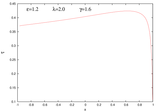
Figure 7: Variation of the ratio of analogue to the actual Hawking temperature $\tau$ with the black hole spin angular momentum (the Kerr parameter $a$).

As mentioned earlier, the discriminant ${\cal D}$ of the corresponding acoustic metric changes sign whenever the state of transonicity of the flow flips from sub- to super-sonicity or vice versa. For multi-transonic shocked accretion flow, such state flipping occurs three times, first, from a sub-sonic to a supersonic state at the outer sonic point (the outer acoustic horizon $r_{h}^{out}$), then from the supersonic to the subsonic state at the shock location through the Rankine-Hugoniot shock, and then from the subsonic to the supersonic state again at the inner sonic point (the inner acoustic horizon $r_{h}^{in}$). A transition from ${\cal D}<0$ (subsonic flow) to ${\cal D}>0$ (supersonic flow) produces an acoustic black hole, while the reverse transition (${\cal D}>0{\longrightarrow}{\cal D}<0$) produces an acoustic white hole (Bercelo, Liberati, Sonego & Visser 2004; Abraham, Bilić & Das 2006). It is thus obvious that for multi-transonic accretion encountering a stable shock, two acoustic black holes are formed, one at the inner and the other at the outer acoustic horizons (the inner and outer sonic points), and an acoustic white hole is produced at the shock. For relativistic accretion disc with constant thickness, this has formally been demonstrated (Abraham, Bilić & Das 2006) by computing the value of ${\cal D}$ for the whole span of $r$ ranging from infinity to the event horizon to demonstrate that the ${\cal D}<0{\longrightarrow}{\cal D}>0$ transition indeed takes place at $r_{s}^{in}$ and at $r_{s}^{out}$, and ${\cal D}>0{\longrightarrow}{\cal D}<0$ transition takes place at the shock location. Similar calculation can also be performed for the disc geometry with the specific form of disc height (81) used in this work.

XIV Black Hole Accretion in ‘Modified’ Newtonian Potentials

Rigorous investigation of the complete general relativistic multi-transonic black hole accretion disc structure is extremely complicated. At the same time it is understood that, as relativistic effects play an important role in the regions close to the accreting black hole (where most of the gravitational potential energy is released), purely Newtonian gravitational potential cannot be a realistic choice to describe transonic black hole accretion in general. To compromise between the ease of handling of a Newtonian description of gravity and the realistic situations described by complicated general relativistic calculations, a series of ‘modified’ Newtonian potentials have been introduced to describe the general relativistic effects that are most important for accretion disk structure around Schwarzschild and Kerr black holes (see Artemova, Björnsson & Novikov 1996; Das 2002, and references therein for further discussion).

Introduction of such potentials allows one to investigate the complicated physical processes taking place in disc accretion in a semi-Newtonian framework by avoiding pure general relativistic calculations so that most of the features of spacetime around a compact object are retained and some crucial properties of the analogous relativistic solutions of disc structure could be reproduced with high accuracy. Hence, those potentials might be designated as ‘pseudo-Kerr’ or ‘pseudo- Schwarzschild’ potentials, depending on whether they are used to mimic the space time around a rapidly rotating or non rotating/ slowly rotating (Kerr parameter $a\sim 0$) black holes respectively. Below we describe four such pseudo Schwarzschild potentials on which we will concentrate in this article. In this section, as well as in the following sections, we will use the value of $r_{g}$ to be equal to $2GM_{BH}/c^{2}$.

It is important to note that as long as one is not interested in astrophysical processes extremely close (within $1-2~{}r_{g}$) to a black hole horizon, one may safely use the following black hole potentials to study accretion on to a Schwarzschild black hole with the advantage that use of these potentials would simplify calculations by allowing one to use some basic features of flat geometry (additivity of energy or de-coupling of various energy components, i.e., thermal ($\frac{c_{s}^{2}}{\gamma-1}$), Kinetic ($\frac{u^{2}}{2}$) or gravitational ($\Phi$) etc., see subsequent discussions) which is not possible for calculations in a purely Schwarzschild or a Kerr metric. Also, one can study more complex many body problems such as accretion from an ensemble of companions or overall efficiency of accretion onto an ensemble of black holes in a galaxy or for studying numerical hydrodynamic accretion flows around a black hole etc. as simply as can be done in a Newtonian framework, but with far better accuracy. So a comparative study of multi-transonic accretion flow using all these potentials might be quite useful in understanding some important features of the analogue properties of astrophysical accretion.

Also, one of the main ‘charms’ of the classical analogue gravity formalism is that even if the governing equations for fluid flow is completely non-relativistic (Newtonian), the propagation of acoustic fluctuations embedded into it are described by a curved pseudo-Riemannian geometry. In connection to astrophysical accretion, one of the best ways to manifest such interesting effect would be to study the analogue effects in the Newtonian and post-Newtonian accretion flow. However, one should be careful in using these potentials because none of these potentials discussed in the subsequent paragraphs are ‘exact’ in a sense that they are not directly derivable from the Einstein equations. These potentials could only be used to obtain more accurate correction terms over and above the pure Newtonian results and any ‘radically’ new results obtained using these potentials should be cross-checked very carefully with the exact general relativistic theory.

Paczyński and Wiita (1980) proposed a pseudo-schwarzschild potential of the form

$$\Phi_{1}=-\frac{1}{2(r-1)}$$ (121)

which accurately reproduces the positions of the marginally stable orbit $r_{s}$ and the marginally bound orbit $r_{b}$, and provides the value of efficiency to be $-0.0625$, which is in close agreement with the value obtained in full general relativistic calculations. Also the Keplarian distribution of angular momentum obtained using this potential is exactly same as that obtained in pure Schwarzschild geometry. It is worth mentioning here that this potential was first introduced to study a thick accretion disc with super Eddington Luminosity. Also, it is interesting to note that although it had been thought of in terms of disc accretion, $\Phi_{1}$ is spherically symmetric with a scale shift of $r_{g}$.

To analyze the normal modes of acoustic oscillations within a thin accretion disc around a compact object (slowly rotating black hole or weakly magnetized neutron star), Nowak and Wagoner (1991) approximated some of the dominant relativistic effects of the accreting black hole (slowly rotating or non-rotating) via a modified Newtonian potential of the form

$$\Phi_{2}=-\frac{1}{2r}\left[1-\frac{3}{2r}+12{\left(\frac{1}{2r}\right)}^{2}\right]$$ (122)

$\Phi_{2}$ has correct form of $r_{s}$ as in the Schwarzschild case but is unable to reproduce the value of $r_{b}$. This potential has the correct general relativistic value of the angular velocity $\Omega_{s}$ at $r_{s}$. Also it reproduces the radial epicyclic frequency $i\nu_{\kappa}$ (for $r>r_{s}$) close to its value obtained from general relativistic calculations, and among all black hole potentials, $\Phi_{2}$ provides the best approximation for $\Omega_{s}$ and $\nu_{\kappa}$. However, this potential gives the value of efficiency as $-0.064$ which is larger than that produced by $\Phi_{1}$, hence the disc spectrum computed using $\Phi_{2}$ would be more luminous compared to a disc structure studied using $\Phi_{1}$.

Considering the fact that the free-fall acceleration plays a very crucial role in Newtonian gravity, Artemova, Björnsson & Novikov (1996) proposed two different black hole potentials to study disc accretion around a non-rotating black hole. The first potential proposed by them produces exactly the same value of the free-fall acceleration of a test particle at a given value of $r$ as is obtained for a test particle at rest with respect to the Schwarzschild reference frame, and is given by

$$\Phi_{3}=-1+{\left(1-\frac{1}{r}\right)}^{\frac{1}{2}}$$ (123)

The second one gives the value of the free fall acceleration that is equal to the value of the covariant component of the three dimensional free-fall acceleration vector of a test particle that is at rest in the Schwarzschild reference frame and is given by

$$\Phi_{4}=\frac{1}{2}ln{\left(1-\frac{1}{r}\right)}$$ (124)

Efficiencies produced by $\Phi_{3}$ and $\Phi_{4}$ are $-0.081$ and $-0.078$ respectively.The magnitude of efficiency produced by $\Phi_{3}$ being maximum,calculation of disc structure using $\Phi_{3}$ will give the maximum amount of energy dissipation and the corresponding spectrum would be the most luminous one. Hereafter we will refer to all these four potentials by $\Phi_{i}$ in general, where $\left\{i=1,2,3,4\right\}$ would correspond to $\Phi_{1}$ (121), $\Phi_{2}$ (122), $\Phi_{3}$ (123) and $\Phi_{4}$ (124) respectively. One should notice that while all other $\Phi_{i}$ have singularity at $r=r_{g}$, only $\Phi_{2}$ has a singularity at $r=0$.

Figure 8: Newtonian potential and other pseudo-potentials $\Phi_{i}(r)$ ($i=1,2,3,4$) are plotted as a function of the logarithmic radial distance from the accreting black hole. This figure is reproduced from Das & Sarkar 2001.

In figure 8 (reproduced from Das & Sarkar 2001), we plot various $\Phi_{i}$ as a function of the radial distance measured from the accreting black hole in units of $r_{g}$. Also in the same plot, purely Newtonian potential is plotted. If we now define a quantity ${\bf S}_{i}$ to be the ‘relative stiffness’ of a potential $\Phi_{i}$ as:

$${\bf S}_{i}=\frac{\Phi_{i}}{r}$$

(that is, ${\bf S}_{i}$ is a measure of the numerical value of any $i$th potential at a radial distance $r$), we find that for $r~{}>~{}2r_{g}$,

$${\bf S}_{2}~{}<~{}{\bf S}_{\rm N}~{}<~{}{\bf S}_{1}~{}<~{}{\bf S}_{3}~{}<~{}{\bf S}_{4},$$

which indicates that while $\Phi_{2}$ is a ‘flatter’ potential compared to the pure Newtonian potential $\Phi_{\rm N}$, all other pseudo potentials are ‘steeper’ to $\Phi_{\rm N}$ for $r~{}>~{}2r_{g}$.
One can write the modulus of free fall acceleration obtained from all ‘pseudo’ potentials except for $\Phi_{2}$ in a compact form as

$$\left|{{{{{\Phi}^{{}^{\prime}}}_{i}}}}\right|=\frac{1}{2{r^{2-{\delta}_{i}}{\left(r-1\right)}^{\delta_{i}}}}$$ (125)

where ${\delta_{1}}=2$, $\delta_{3}=\frac{1}{2}$ and $\delta_{4}=1$. $\left|{{{{{\Phi}^{{}^{\prime}}}_{i}}}}\right|$ denotes the absolute value of the space derivative of $\Phi_{i}$, i.e.,

$$\left|{{{{{\Phi}^{{}^{\prime}}}_{i}}}}\right|=\left|{\frac{d{\Phi_{i}}}{dr}}\right|$$

whereas acceleration produced by $\Phi_{2}$ can be computed as,

$${\Phi_{2}}^{{}^{\prime}}=\frac{1}{2r^{2}}\left(1-\frac{3}{r}+\frac{9}{2r^{2}}\right)$$ (126)

For axisymmetric accretion, at any radial distance $r$ measured from the accretor, one can define the effective potential $\Phi_{i}^{eff}(r)$ to be the summation of the gravitational potential and the centrifugal potential for matter accreting under the influence of $i$th pseudo potential. $\Phi_{i}^{eff}(r)$ can be expressed as:

$$\Phi_{i}^{eff}(r)=\Phi_{i}(r)+\frac{\lambda^{2}(r)}{2r^{2}}$$ (127)

where $\lambda(r)$ is the non-constant distance dependent specific angular momentum of accreting material. One then easily shows that $\lambda(r)$ may have an upper limit:

$$\lambda^{up}_{i}(r)=r^{\frac{3}{2}}\sqrt{\Phi^{{}^{\prime}}_{i}(r)}$$ (128)

where $\Phi^{{}^{\prime}}_{i}(r)$ represents the derivative of $\Phi_{i}(r)$ with respect to $r$. For weakly viscous or inviscid flow, angular momentum can be taken as a constant parameter ($\lambda$) and (127) can be approximated as:

$$\Phi_{i}^{eff}(r)=\Phi_{i}(r)+\frac{\lambda^{2}}{2r^{2}}$$ (129)

For general relativistic treatment of accretion, the effective potential can not be decoupled in to its gravitational and centrifugal components. The general relativistic effective potential $\Phi^{eff}_{GR}(r)$ (excluding the rest mass) experienced by the fluid accreting on to a Schwarzschild black hole can be expressed as:

$$\Phi^{eff}_{GR}(r)=r\sqrt{\frac{r-1}{r^{3}-{\lambda}^{2}\left(1+r\right)}}-1$$ (130)

One can understand that the effective potentials in general relativity cannot be obtained by linearly combining its gravitational and rotational contributions because various energies in general relativity are combined together to produce non-linearly coupled new terms.

Figure 9: ($\Phi_{BH}^{eff}(r)$) as well as for pseudo-general relativistic($\Phi^{eff}_{i}(r)$) accretion discs as a function of the distance (measured from the event horizon in units or $r_{g}$) plotted in logarithmic scale. The specific angular momentum is chosen to be 2 in geometric units. The figure is reproduced from Das 2002.

In Fig. 9. (reproduced from Das 2002), we plot $\Phi_{i}^{eff}(r)$ (obtained from (129)) and $\Phi^{eff}_{GR}(r)$ as a function of $r$ in logarithmic scale. The value of $\lambda$ is taken to be 2 in units of $2GM/c$. $\Phi^{eff}$ curves for different $\Phi_{i}$ are marked exclusively in the figure and the curve marked by ${\bf G^{R}}$ represents the variation of $\Phi^{eff}_{GR}(r)$ with $r$. One can observe that $\Phi^{eff}_{1}(r)$ is in excellent agreement with $\Phi^{eff}_{GR}(r)$. Only for a very small value of $r$ ($r{\rightarrow}r_{g}$), $\Phi^{eff}_{1}$ starts deviating from $\Phi^{eff}_{GR}(r)$ and this deviation keeps increasing as matter approaches closer and closer to the event horizon. All other $\Phi^{eff}_{i}(r)$s approaches to $\Phi^{eff}_{GR}(r)$ at a radial distance (measured from the black hole) considerably larger compared to the case for $\Phi^{eff}_{1}(r)$. If one defines ${\Delta}_{i}^{eff}(r)$ to be the measure of the deviation of $\Phi^{eff}_{i}(r)$ with $\Phi^{eff}_{GR}(r)$ at any point $r$,

$${\Delta}_{i}^{eff}(r)=\Phi^{eff}_{i}(r)-\Phi^{eff}_{GR}(r)$$

One observes that ${\Delta}_{i}^{eff}(r)$ is always negative for $\Phi^{eff}_{1}(r)$, but for other $\Phi^{eff}_{i}(r)$, it normally remains positive for low values of $\lambda$ but may become negative for a very high value of $\lambda$. If ${{|}}{\Delta}_{i}^{eff}(r){{|}}$ be the modules or the absolute value of ${\Delta}_{i}^{eff}(r)$, one can also see that, although only for a very small range of radial distance very close to the event horizon, ${\Delta}_{3}^{eff}(r)$ is maximum, for the whole range of distance scale while $\Phi_{1}$ is the best approximation of general relativistic space time, $\Phi_{2}$ is the worst approximation and $\Phi_{4}$ and $\Phi_{3}$ are the second and the third best approximation as long as the total effective potential experienced by the accreting fluid is concerned. It can be shown that ${{|}}{\Delta}_{i}^{eff}(r){{|}}$ nonlinearly anti-correlates with $\lambda$. The reason behind this is understandable. As $\lambda$ decreases, rotational mass as well as its coupling term with gravitational mass decreases for general relativistic accretion material while for accretion in any $\Phi_{i}$, centrifugal force becomes weak and gravity dominates; hence deviation from general relativistic case will be more prominent because general relativity is basically a manifestation of strong gravity close to the compact objects.
From the figure it is clear that for $\Phi^{eff}_{GR}(r)$ as well as for all $\Phi^{eff}_{i}(r)$, a peak appears close to the horizon. The height of these peaks may roughly be considered as the measure of the strength of the centrifugal barrier encountered by the accreting material for respective cases. The deliberate use of the word ‘roughly’ instead of ‘exactly’ is due to the fact that here we are dealing with fluid accretion, and unlike particle dynamics, the distance at which the strength of the centrifugal barrier is maximum, is located further away from the peak of the effective potential because here the total pressure contains the contribution due to fluid or ‘ram’ pressure also. Naturally the peak height for $\Phi^{eff}_{GR}(r)$ as well as for $\Phi^{eff}_{i}(r)$ increases with increase of $\lambda$ and the location of this barrier moves away from the black hole with higher values of angular momentum. If the specific angular momentum of accreting material lies between the marginally bound and marginally stable value, an accretion disc is formed. For inviscid or weakly viscous flow, the higher will be the value of $\lambda$, the higher will be the strength of the centrifugal barrier and the more will be the amount of radial velocity or the thermal energy that the accreting material must have to begin with so that it can be made to accrete on to the black hole. In this connection it is important to observe from the figure that accretion under $\Phi_{1}(r)$ will encounter a centrifugal barrier farthest away from the black hole compared to other $\Phi_{i}$. For accretion under all $\Phi_{i}$s except $\Phi_{1}$,the strength of centrifugal barrier at a particular distance will be more compared to its value for full general relativistic accretion.

In subsequent sections, we will use the above mentioned potentials to study the analogue effects in spherically symmetric and in axisymmetric black hole accretion.

XV Newtonian and Post-Newtonian Spherical Accretion as an Analogue Model

In this section, we study the analogue gravity phenomena in the spherical accretion onto astrophysical black holes under the influence of Newtonian as well as various post-Newtonian pseudo-Schwarzschild potentials described above. We use the expressions ‘post-Newtonian’ and ‘pseudo-Schwarzschild’ synonymously. Our main goal is to provide a self-consistent calculation of the analogue horizon temperature $T_{\rm AH}$ in terms of the minimum number of physical accretion parameters, and to study the dependence of $T_{\rm AH}$ on various flow properties. This section is largely based on Dasgupta, Bilić & Das 2005.

XV.1 Equation of Motion

The non-relativistic equation of motion for spherically accreting matter in a gravitational potential denoted by $\Phi$ may be written as

$$\frac{{\partial{u}}}{{\partial{t}}}+u\frac{{\partial{u}}}{{\partial{r}}}+\frac{1}{\rho}\frac{{\partial}p}{{\partial}r}+\frac{{\partial}\Phi}{\partial{r}}=0,$$ (131)

The first term in (131) is the Eulerian time derivative of the dynamical velocity, the second term is the ‘advective’ term, the third term is the momentum deposition due to the pressure gradient and the last term is the gravitational force. Another equation necessary to describe the motion of the fluid is the continuity equation

$$\frac{{\partial}{\rho}}{{\partial}t}+\frac{1}{r^{2}}\frac{{\partial}}{{\partial}r}\left({\rho}ur^{2}\right)=0.$$ (132)

To integrate the above set of equations, one also needs the equation of state that specifies the intrinsic properties of the fluid. We will study accretion described by either a polytropic or an isothermal equation of state.

XV.2 Sonic Quantities

XV.2.1 Polytropic Accretion

We employ a polytropic equation of state of the form $p=K{\rho}^{\gamma}$. The sound speed $c_{s}$ is defined by

$$c_{s}^{2}\equiv\left.\frac{\partial p}{\partial\rho}\right|_{\rm constant~{}~{}entropy}=\gamma\frac{p}{\rho},$$ (133)

Assuming stationarity of the flow, we find the following conservation equations:

1) Conservation of energy implies constancy of the specific energy ${\cal E}$

$${\cal E}=\frac{u^{2}}{2}+\frac{c_{s}^{2}}{{\gamma}-1}+\Phi.$$ (134)

2) Conservation of the baryon number implies constancy of the accretion rate ${\dot{M}}$

$${\dot{M}}=4{\pi}{\rho}ur^{2}.$$ (135)

Equation (134) is obtained from (131), and (135) follows directly from (132).

Substituting $\rho$ in terms of $c_{s}$ and differentiating (135) with respect to $r$, we obtain

$$c_{s}^{\prime}=\frac{c_{s}(1-\gamma)}{2}\left(\frac{u^{\prime}}{u}+\frac{2}{r}\right),$$ (136)

where ^′ denotes the derivative with respect to $r$. Next we differentiate (134) and eliminating $c_{s}^{\prime}$ with the help of (136) we obtain

$$u^{\prime}=\frac{2c_{s}^{2}/r-\Phi^{\prime}}{u-c_{s}^{2}/u}\,.$$ (137)

One thus finds the critical point conditions as

$${u}_{\rm r=r_{c}}={c_{s}}_{\rm r=r_{c}}=\sqrt{\left|\frac{r\Phi^{\prime}}{2}\right|_{\rm r=r_{c}}}\,,$$ (138)

As described in section 12.2, here also the critical point and the sonic points are equivalent, and the location of the sonic point is identical to the location of the acoustic horizon due to the assumption of stationarity and spherical symmetry. Thus, hereafter we denote $r_{h}$ as the sonic point and the sphere of radius $r_{h}$ as the acoustic horizon. Hereafter, the subscript $h$ indicates that a particular quantity is evaluated at $r_{h}$. The location of the acoustic horizon is obtained by solving the algebraic equation

$${\cal E}-\frac{1}{4}\left(\frac{\gamma+1}{\gamma-1}\right)r_{h}{\Phi^{\prime}_{h}}-{\Phi_{h}}=0.$$ (139)

The derivative $u^{\prime}_{h}$ at the corresponding sonic point is obtained by solving the quadratic equation

$$\left(1+\gamma\right)\left(u^{\prime}_{h}\right)^{2}+2\left(\gamma-1\right)\sqrt{\frac{2\Phi^{\prime}_{h}}{r_{h}}}\,u^{\prime}_{h}$$

$$+\left(2{\gamma}-1\right)\frac{\Phi^{\prime}_{h}}{r_{h}}+{\Phi^{\prime\prime}_{h}} = 0,$$ (140)

which follows from (137) in the limit $r{\rightarrow}r_{h}$ evaluated with the help of l’Hospital’s rule.

Finally, the gradient of the sound speed at the acoustic horizon is obtained by substituting $u^{\prime}_{h}$ obtained from (140) into equation (136) at the acoustic horizon

$$\left.c_{s}^{\prime}\right|_{h}=\left(\frac{1-\gamma}{2}\right)\left(u^{\prime}_{h}+\sqrt{\frac{2\Phi^{\prime}_{h}}{r_{h}}}\right).$$ (141)

XV.2.2 Isothermal Accretion

We employ the isothermal equation of state of the form

$$p=\frac{RT}{\mu}\rho=c_{s}^{2}{\rho}\,,$$ (142)

where $T$ is the temperature, $R$ and $\mu$ are the universal gas constant and the mean molecular weight, respectively. The quantity $c_{s}$ is the isothermal sound speed defined by

$$c_{s}^{2}=\left.\frac{\partial p}{\partial\rho}\right|_{T}={\Theta}T\,,$$ (143)

where the derivative is taken at fixed temperature and the constant $\Theta=\kappa_{B}/(\mu m_{H})$ with $m_{H}\simeq m_{p}$ being the mass of the hydrogen atom. In our model we assume that the accreting matter is predominantly hydrogen, hence $\mu\simeq 1$. Now, the specific energy equation takes the form

$${\cal E}=\frac{u^{2}}{2}+{\Theta}T\ln\rho+\Phi\,,$$ (144)

whereas the accretion rate is given by (135) as before.

The radial change rate of the dynamical velocity is again given by (137). From (137) and with (143) we find the sonic point condition as

$$u_{h}=\sqrt{\frac{r_{h}\Phi^{\prime}_{h}}{2}}=c_{s}=\sqrt{{\Theta}T}\,.$$ (145)

since $c_{s}$ does not depend on $r$. The derivative of $u$ at $r_{h}$ is obtained from (137) by making use of l’Hospital’s rule as before. We find

$$u^{\prime}_{h}=-\sqrt{-\frac{1}{2}\left(\frac{1}{r_{h}}\Phi^{\prime}_{h}+\Phi^{\prime\prime}_{h}\right)}\,,$$ (146)

where the minus sign in front of the square root indicates accretion (the plus would correspond to a wind solution). Note that the quantities in equations (145) and (146) are functions of the fluid temperature $T$ only. Hence the isothermal spherical accretion can be essentially described as a one-parameter solution of the hydrodynamical equations, parameterized by $T$.

XV.3 Analogue Temperature

From (33) in Newtonian limit, i.e.,

$$|\chi^{2}|=g_{00}\rightarrow{\left(1+\frac{\Phi}{2c^{2}}\right)}$$ (147)

gives a general expression for the temperature of the analogue Hawking radiation in a spherically accreting fluid in the Newtonian as well as in any pseudo-Schwarzschild gravitational potential

$$T_{\rm AH}=\frac{\hbar}{2{\pi}\kappa_{b}}\sqrt{\frac{2c^{2}+\Phi_{h}}{2c^{2}}}\left[\frac{1}{1-c_{s}^{2}}\left|\frac{d}{dr}\left(c_{s}-u\right)\right|\right]_{\rm r=r_{h}}\,.$$ (148)

The quantities required to calculate the analogue temperature (148) are obtained using the formalism presented in section 15.2. For polytropic accretion, using equations (136)-(141) one finds

$$\tau\equiv\frac{T_{\rm AH}}{T_{\rm H}}=4\sqrt{\frac{2+\Phi_{h}}{2}}\left(\frac{2}{2-r_{h}\Phi_{h}}\right)\left(\frac{\gamma+1}{2}\right)$$

$$\sqrt{\frac{\Phi^{\prime}_{h}}{r_{h}}{\bf f}(\gamma)-\left(1+\gamma\right)\Phi^{\prime\prime}_{h}}$$ (149)

where ${\bf f}(\gamma)=\left(0.00075\gamma^{2}-5.0015{\gamma}+3.00075\right)$. The quantities $\Phi_{h}$, $\Phi^{\prime}_{h}$, and $\Phi^{\prime\prime}_{h}$ are obtained by calculating the values of various potentials at $r_{h}$, and $r_{h}$ is calculated from (139) for an astrophysically relevant choice of $\{{\cal E},\gamma\}$.

Note that if $(c_{s}^{\prime}-u^{\prime})_{h}$ is negative, one obtains an acoustic white-hole solution. Hence the condition for the existence of the acoustic white hole is

$$\left(\frac{\gamma+1}{2}\right)\sqrt{\frac{\Phi^{\prime}_{h}}{r_{h}}{\bf f}(\gamma)-\left(1+\gamma\right)\Phi^{\prime\prime}_{h}}\><0.$$ (150)

Since $\gamma$ and $r_{h}$ can never be negative, and since $\Phi^{\prime\prime}_{h}$ and $\Phi^{\prime\prime}_{h}$ are always real for the preferred domain of $\{{\cal E},\gamma\}$, unlike general relativistic spherical accretion, acoustic white-hole solutions are excluded in the astrophysical accretion governed by the Newtonian or post-Newtonian potentials.

For an isothermal flow, the quantity $c_{s}^{\prime}$ is zero and using (146) we find

$$\tau=4\sqrt{2}\left(\frac{1}{2-r_{h}\Phi^{\prime}_{h}}\right)\sqrt{-\left(1+\frac{\Phi_{h}}{2}\right)\left(\Phi^{\prime\prime}_{h}+\frac{\Phi^{\prime}_{h}}{r_{h}}\right)}\,,$$ (151)

where $r_{h}$ should be evaluated using (145). Clearly, the fluid temperature $T$ completely determines the analogue Hawking temperature. Hence, a spherical isothermally accreting astrophysical black hole provides a simple system where analogue gravity can be theoretically studied using only one free parameter.

For both polytropic and isothermal accretion, for certain range of the parameter space, the analogue Hawking temperature $T_{AH}$ may become higher than the actual Hawking temperature $T_{H}$, see Dasgupta, Bilić & Das 2005 for further details.

XVI Post-Newtonian Multi-transonic Accretion Disc as Analogue Model

In this section, we will study the analogue gravity phenomena for polytropic (adiabatic) and isothermal rotating, advective, multi-transonic accretion disc in various pseudo-Schwarzschild potentials described in section 14.

XVI.1 Flow Dynamics and Accretion Variables at the Critical Point

XVI.1.1 Polytropic Accretion

The local half-thickness, $h_{i}(r)$ of the disc for any $\Phi_{i}$ can be obtained by balancing the gravitational force by pressure gradient and can be expressed as:

$$h_{i}(r)=c_{s}\sqrt{{r}/\left({\gamma}{\Phi_{i}^{\prime}}\right)}$$ (152)

where $\Phi_{i}^{\prime}=d\Phi_{i}/dr$. For a non-viscous flow obeying the polytropic equation of state $p=K{\rho}^{\gamma}$, integration of radial momentum equation:

$$u\frac{{d{u}}}{{d{r}}}+\frac{1}{\rho}\frac{{d}P}{{d}r}+\frac{d}{dr}\left(\Phi^{eff}_{i}(r)\right)=0$$ (153)

leads to the following energy conservation equation (on the equatorial plane of the disc) in steady state:

$${\cal E}=\frac{1}{2}u^{2}+\frac{c_{s}^{2}}{\gamma-1}+\frac{{\lambda}^{2}}{2r^{2}}+\Phi_{i}$$ (154)

and the continuity equation:

$$\frac{{d}}{{d}r}\left[u{\rho}rh_{i}(r)\right]=0$$ (155)

can be integrated to obtain the baryon number conservation equation:

$${\dot{M}}=\sqrt{\frac{1}{\gamma}}uc_{s}{\rho}r^{\frac{3}{2}}\left({\Phi_{i}^{\prime}}\right)^{-\frac{1}{2}}.$$ (156)

The entropy accretion rate ${\dot{\Xi}}$ can be expressed as:

$${\dot{\Xi}}=\sqrt{\frac{1}{\gamma}}uc_{s}^{\left({\frac{\gamma+1}{\gamma-1}}\right)}r^{\frac{3}{2}}\left({\Phi_{i}^{\prime}}\right)^{-\frac{1}{2}}$$ (157)

One can simultaneously solve (154) and (157) for any particular $\Phi_{i}$ and for a particular set of values of $\left\{{\cal E},\lambda,\gamma\right\}$. For a particular value of $\left\{{\cal E},\lambda,\gamma\right\}$, it is now quite straight-forward to derive the space gradient of the acoustic velocity $\left(\frac{dc_{s}}{dr}\right)_{i}$ and the dynamical flow velocity $\left(\frac{du}{dr}\right)_{i}$ for flow in any particular $i$th black hole potential $\Phi_{i}$:

$$\left(\frac{dc_{s}}{dr}\right)_{i}=c_{s}\left(\frac{\gamma-1}{\gamma+1}\right)\left(\frac{1}{2}\frac{{\Phi_{i}}^{{\prime}{\prime}}}{{\Phi_{i}}^{{\prime}}}-\frac{3}{2r}-\frac{1}{u}\frac{du}{dr}\right)$$ (158)

and,

$$\left(\frac{du}{dr}\right)_{i}=\frac{\left(\frac{\lambda^{2}}{r^{3}}+\Phi^{{}^{\prime}}_{i}(r)\right)-\frac{c_{s}^{2}}{\gamma+1}\left(\frac{3}{r}+\frac{\Phi^{{}^{\prime\prime}}_{i}(r)}{\Phi^{{}^{\prime}}_{i}(r)}\right)}{u-\frac{2c_{s}^{2}}{u\left(\gamma+1\right)}}$$ (159)

where ${\Phi_{i}}^{{\prime}{\prime}}$ represents the derivative of ${\Phi_{i}}^{{\prime}}$. Hence the critical point condition comes out to be:

$$\left[c_{s}^{i}\right]_{\rm r=r_{c}}=\sqrt{\frac{1+\gamma}{2}}\left[u^{i}\right]_{\rm r=r_{c}}=\left[\frac{\Phi^{{}^{\prime}}_{i}(r)+{\gamma}\Phi^{{}^{\prime}}_{i}(r)}{r^{2}}\left(\frac{\lambda^{2}+r^{3}\Phi^{{}^{\prime}}_{i}(r)}{3\Phi^{{}^{\prime}}_{i}(r)+r\Phi^{{}^{\prime\prime}}_{i}(r)}\right)\right]_{\rm r=r_{c}}$$ (160)

Note that the Mach number $M_{c}$ at the critical point is not equal to unity, rather:

$$M_{c}=\sqrt{\frac{2}{\gamma+1}}$$ (161)

Hence, the critical points and the sonic points are not equivalent. One needs to calculate the sonic point, which is the location of the acoustic horizon, following the procedure as described in section 13.5.

For any fixed set of $\left\{{\cal E},\lambda,\gamma\right\}$, the critical points can be obtained by solving the following polynomial of $r$:

$${\cal E}-{\left[\frac{\lambda^{2}}{2r^{2}}+\Phi_{i}\right]}_{\rm r=r_{c}}-\frac{2\gamma}{\gamma^{2}-1}\left[\frac{\Phi^{{}^{\prime}}_{i}(r)+{\gamma}\Phi^{{}^{\prime}}_{i}(r)}{r^{2}}\left(\frac{\lambda^{2}+r^{3}\Phi^{{}^{\prime}}_{i}(r)}{3\Phi^{{}^{\prime}}_{i}(r)+r\Phi^{{}^{\prime\prime}}_{i}(r)}\right)\right]_{\rm r=r_{c}}=0.$$ (162)

The dynamical velocity gradient at the critical point can be obtained by solving the following equation for $(du/dr)_{\rm r=r_{c}}$:

$$\frac{4{\gamma}}{\gamma+1}\left(\frac{du}{dr}\right)^{2}_{c,i}-2\left|u\right|_{\rm r=r_{c}}\frac{\gamma-1}{\gamma+1}\left[\frac{3}{r}+\frac{\Phi^{{}^{\prime\prime}}_{i}(r)}{\Phi^{{}^{\prime}}_{i}(r)}\right]_{\rm r=r_{c}}\left(\frac{du}{dr}\right)_{c,i}$$

$$+\left|c^{2}_{s}\left[\frac{\Phi^{{}^{\prime\prime\prime}}_{i}(r)}{\Phi^{{}^{\prime}}_{i}(r)}-\frac{2\gamma}{\left(1+{\gamma}\right)^{2}}\left(\frac{\Phi^{{}^{\prime\prime}}_{i}(r)}{\Phi^{{}^{\prime}}_{i}(r)}\right)^{2}+\frac{6\left(\gamma-1\right)}{\gamma{\left(\gamma+1\right)^{2}}}\left(\frac{\Phi^{{}^{\prime\prime}}_{i}(r)}{\Phi^{{}^{\prime}}_{i}(r)}\right)-\frac{6\left(2\gamma-1\right)}{\gamma^{2}{\left(\gamma+1\right)^{2}}}\right]\right|_{\rm r=r_{c}}$$

$$+\Phi^{{}^{\prime\prime}}_{i}{\Bigg{|}}_{\rm r=r_{c}}-\frac{3\lambda^{2}}{r^{4}_{c}}=0$$ (163)

Where the subscript $(c,i)$ indicates that the corresponding quantities for any $i$th potential is being measured at its corresponding critical point and $\Phi^{{}^{\prime\prime\prime}}_{i}=\frac{d^{3}\Phi_{i}}{dr^{3}}$.

XVI.1.2 Isothermal Accretion

The isothermal sound speed is defined as:

$$c_{s}={\Theta}T^{\frac{1}{2}}$$ (164)

where $\Theta=\sqrt{\frac{\kappa_{B}{\mu}}{m_{H}}}$ is a constant, ${m_{H}}{\sim}{m_{P}}$ being the mass of the hydrogen atom and $\kappa_{B}$ is Boltzmann’s constant. The local half-thickness $h_{i}(r)$ of the disc for any $\Phi_{i}(r)$ can be obtained by balancing the gravitational force by pressure gradient and can be expressed as

$$h_{i}(r)=\Theta{\sqrt{\frac{rT}{\Phi_{i}^{\prime}{}}}}$$ (165)

Solution of the radial momentum conservation equation and the continuity equation provides the following two integral of motion on the equatorial plane of the isothermal accretion disc

$$\frac{u^{2}(r)}{2}+{\Theta}Tln{\rho(r)}+\frac{\lambda^{2}}{2r^{2}}+\Phi_{i}={\rm Constant}$$ (166)

and

$${\dot{M}}={\Theta}{\rho}(r)u(r)r^{\frac{3}{2}}\sqrt{\frac{T}{\Phi_{i}^{\prime}}}$$ (167)

The dynamical flow velocity for a particular value of $\left\{{\cal E},\lambda\right\}$ can be expressed as

$$\frac{du}{dr}=\left[\frac{\left(\frac{3\Theta^{2}T}{2r}+\frac{\lambda^{2}}{r^{3}}\right)-\left(\frac{1}{2}\Theta^{2}T\frac{\Phi_{i}^{\prime\prime}(r)}{\Phi_{i}^{\prime}(r)}+\Phi_{i}^{\prime}\right)}{\left(u-\frac{\Theta^{2}T}{u}\right)}\right]$$ (168)

where $\Phi_{i}^{\prime\prime}=\frac{d^{2}\Phi_{i}}{dr^{2}}$. Since the flow is isothermal, $dc_{s}/dr=0$ everywhere identically.

The critical point condition can be expressed as:

$$\left|u\right|_{\rm r=r_{c}}=\Theta{T^{\frac{1}{2}}}=\sqrt{\frac{{\Phi_{i}^{\prime}}{\Bigg{|}}_{\rm r=r_{c}}-\frac{\lambda^{2}}{r_{c}^{3}}}{\frac{3}{2r_{c}}-\frac{1}{2}\left(\frac{{\Phi_{i}}^{\prime\prime}}{\Phi_{i}^{\prime}}\right)_{\rm r=r_{c}}}}$$ (169)

Note that the Mach number at the critical point is exactly equal to unity, hence the critical points and the sonic points are identical for isothermal accretion disc. Therefore, $r_{c}$ is actually the location of the acoustic event horizon $r_{h}$, and for a specific value of $\left\{{\cal E},\lambda\right\}$, $r_{h}$ can be computed by solving the following equation for $r_{h}$:

$$\Phi_{i}^{\prime\prime}{\Bigg{|}}_{\rm r=r_{h}}+\frac{2}{\Theta^{2}T}\left(\Phi_{i}^{\prime}\right)_{\rm r=r_{h}}^{2}-\left[\frac{3}{r_{h}\Theta}+\frac{2{\lambda}^{2}}{T{\Theta}^{2}r_{h}^{3}}\right]\Phi_{i}^{\prime}{\Bigg{|}}_{\rm r=r_{h}}=0$$ (170)

The dynamical velocity gradient at the acoustic horizon can be obtained as:

$$\left(\frac{du}{dr}\right)_{h,i}=\pm\frac{1}{\sqrt{2}}\left\{\frac{1}{2}\Theta^{2}T{\Bigg{[}}\left(\frac{\Phi_{i}^{\prime\prime}}{\Phi_{i}^{\prime}}\right)_{\rm r=r_{h}}^{2}-\left(\frac{\Phi_{i}^{\prime\prime\prime}}{\Phi_{i}^{\prime}}\right)_{\rm r=r_{h}}\right]$$

$$-\left(\Phi_{i}^{\prime\prime}\Big{|}_{\rm r=r_{h}}+\frac{3\Theta^{2}T}{2r_{h}^{2}}+\frac{3\lambda^{2}}{r_{h}^{4}}\right){\Bigg{\}}}^{\frac{1}{2}}$$ (171)

XVI.2 Multi-transonicity and Shock Formation

As in the case of general relativistic accretion disc, axisymmetric accretion under the influence of a generalized pseudo-Schwarzschild potential $\Phi_{i}$ also produces multiple critical/sonic points, both for polytropic as well as for the isothermal flow. For polytropic flow, (162) can be solved to obtain various critical points, and the flow equations can be integrated from such critical points to find the corresponding sonic points.

For accretion/wind solutions under the influence of various $\Phi_{i}$, one can define the square of the eigenvalue $\bar{\Omega}$ in the following way (Chaudhury, Ray & Das 2006):

$${\bar{\Omega}}^{2}=\frac{4r_{\mathrm{c}}\Phi^{\prime}(r_{\mathrm{c}})|c_{\mathrm{s}}^{2}|_{\rm r=r_{c}}}{(\gamma+1)^{2}}\left[\left(\gamma-1\right){\mathcal{A}}-2\gamma\left(1+{\mathcal{C}}\right)+2\gamma\frac{\mathcal{BC}}{\mathcal{A}}\right]$$

$$-\frac{\lambda^{2}}{\lambda_{\mathrm{K}}^{2}(r_{\mathrm{c}})}\left[4\gamma+\left(\gamma-1\right){\mathcal{A}}+2\gamma\frac{\mathcal{BC}}{\mathcal{A}}\right]$$ (172)

where

$${\cal A}=r_{\rm c}\frac{\Phi^{\prime\prime}(r_{\rm c})}{\Phi^{\prime}(r_{\rm c})}-3,~{}{\cal B}=1+r_{\rm c}\frac{\Phi^{\prime\prime\prime}(r_{\rm c})}{\Phi^{\prime\prime}(r_{\rm c})}-r_{\rm c}\frac{\Phi^{\prime\prime}(r_{\rm c})}{\Phi^{\prime}(r_{\rm c})},~{}{\cal C}={\cal A}+3,~{}\lambda_{\rm K}^{2}(r)=r^{3}\Phi^{\prime}(r)$$ (173)

For isothermal flows, a similar expression for the related eigenvalues may likewise be derived. The algebra in this case is much simpler and it is an easy exercise to assure oneself that for isothermal flows one simply needs to set $\gamma=1$ in (172), to arrive at a corresponding relation for ${\bar{\Omega}}^{2}$.

A generic conclusion that can be drawn about the critical points from the form of ${\bar{\Omega}}^{2}$ in (172), is that for a conserved pseudo-Schwarzschild axisymmetric flow driven by any potential, the only admissible critical points will be saddle points and centre-type points. For a saddle point, ${\bar{\Omega}}^{2}>0$, while for a centre-type point, ${\bar{\Omega}}^{2}<0$. Once the behaviour of all the physically relevant critical points has been understood in this way, a complete qualitative picture of the flow solutions passing through these points (if they are saddle points), or in the neighbourhood of these points (if they are centre-type points), can be constructed, along with an impression of the direction that these solutions can have in the phase portrait of the flow, see Chaudhury, Ray & Das (2006) for further detail.

Application of the above mentioned methodology for finding out the nature of the critical point leads to the conclusion that for multi-transonic accretion and wind, the inner critical point $r_{c}^{in}$ and the outer critical point $r_{c}^{out}$ are of saddle type (‘X’ type), whereas the middle critical point $r_{c}^{mid}$ is of centre type (‘O’ type). For mono-transonic accretion, the critical point will always be of saddle type and will be located either quite close to the event horizon (mono-transonic accretion passing through the ‘inner type’ critical point) or quite far away from the black hole (mono-transonic accretion passing through the ‘outer type’ critical point).

Hereafter we will use the notation $\left[{\cal P}_{i}\right]$ for a set of values of $\left[{\cal E},\lambda,\gamma\right]$ for polytropic accretion in any particular $\Phi_{i}$. For all $\Phi_{i}$, one finds a significant region of parameter space spanned by $\left[{\cal P}_{i}\right]$ which allows the multiplicity of critical points for accretion as well as for wind where two real physical inner and outer (with respect to the location of the black hole event horizon) saddle type critical points $r_{c}^{in}$ and $r_{c}^{out}$ encompass one centre type unphysical middle sonic point $r_{c}^{mid}$ in between. For a particular $\Phi_{i}$, if ${\cal A}_{i}\left[{\cal P}_{i}\right]$ denotes the universal set representing the entire parameter space covering all values of $\left[{\cal P}_{i}\right]$, and if ${\cal B}_{i}\left[{\cal P}_{i}\right]$ represents one particular subset of ${\cal A}_{i}\left[{\cal P}_{i}\right]$ which contains only the particular values of $\left[{\cal P}_{i}\right]$ for which the above mentioned three critical points are obtained, then ${\cal B}_{i}\left[{\cal P}_{i}\right]$ can further be decomposed into two subsets ${\cal C}_{i}\left[{\cal P}_{i}\right]$ and ${\cal D}_{i}\left[{\cal P}_{i}\right]$ such that:

$${\cal C}_{i}\left[{\cal P}_{i}\right]~{}\subseteq~{}{\cal B}_{i}\left[{\cal P}_{i}\right]~{}~{}~{}{\rm\underline{only~{}for}}~{}~{}~{}{\dot{\Xi}}\left(r_{c}^{in}\right)>{\dot{\Xi}}\left(r_{c}^{out}\right)$$

$${\cal D}_{i}\left[{\cal P}_{i}\right]~{}\subseteq~{}{\cal B}_{i}\left[{\cal P}_{i}\right]~{}~{}~{}{\rm\underline{only~{}for}}~{}~{}~{}{\dot{\Xi}}\left(r_{c}^{in}\right)<{\dot{\Xi}}\left(r_{c}^{out}\right)$$ (174)

then for $\left[{\cal P}_{i}\right]\in{\cal C}_{i}\left[{\cal P}_{i}\right]$, we get multi-transonic accretion and for $\left[{\cal P}_{i}\right]\in{\cal D}_{i}\left[{\cal P}_{i}\right]$ one obtains multi-transonic wind.

Figure 10: The complete classification of $\left[{\cal E},\lambda\right]$ for polytropic accretion in the Paczyński & Wiita (1980) potential $\Phi_{1}$. The value of $\gamma$ is taken to be equal to $4/3$. Mono-transonic regions are marked by I (accretion through the inner sonic point only) and O (accretion through the outer sonic point only). The regions marked by ${\cal A}$ and ${\cal W}$ represents the multi-transonic accretion and wind, respectively. The shaded region represents the collection of $\left[{\cal E},\lambda\right]$ (for $\gamma=4/3$) for which the stable Rankine-Hugoniot shock solutions are obtained.

For the Paczyński & Wiita (1980) potential $\Phi_{1}$, in figure 10 we classify the whole $\left[{\cal E},\lambda\right]$ parameter space for a fixed value of $\gamma=4/3$. The region marked by I represents the values of $\left[{\cal E},\lambda\right]$ for which accretion will be mono-transonic and will pass through the saddle type inner critical point, whereas the region marked by O represents the values of $\left[{\cal E},\lambda\right]$ for which accretion will be mono-transonic and will pass through the saddle type outer critical point. The wedge shaped region bounded by heavy solid lines and marked by ${\cal A}$ (including the shaded region) represents the multi-transonic accretion zone for which $\left({\cal E}_{i},\lambda_{i}\right)\in\left[{\cal P}_{i}\right]\in{\cal C}_{i}\left[{\cal P}_{i}\right]~{}\subseteq~{}{\cal B}_{i}\left[{\cal P}_{i}\right]$, whereas the wedge shaped region bounded by the heavy solid line and marked by ${\cal W}$ represents the multi-transonic wind and mono-transonic accretion zone for which $\left({\cal E}_{i},\lambda_{i}\right)\in\left[{\cal P}_{i}\right]\in{\cal D}_{i}\left[{\cal P}_{i}\right]~{}\subseteq~{}{\cal B}_{i}\left[{\cal P}_{i}\right]$. A similar kind of parameter space division can easily be obtained for other $\Phi_{i}$ as well, see Das 2002 and Chaudhury, Ray & Das 2006 for further detail.

If shock forms in accretion, then $\left[{\cal P}_{i}\right]$ responsible for shock formation must be somewhere from the region for which $\left[{\cal P}_{i}\right]\in{\cal C}_{i}\left[{\cal P}_{i}\right]$, though not all $\left[{\cal P}_{i}\right]\in{\cal C}_{i}\left[{\cal P}_{i}\right]$ will allow shock transition. One can derive (see Das 2002 for further detail) the Rankine-Hugoniot shock condition for the generalized potential $\Phi_{i}$ in the following form which will be satisfied only at the shock location

$$\left(1-\gamma\right)\left(\frac{{\rho_{-}}{{\dot{\Xi}}_{-}}}{\dot{M}}\right)^{log_{\Gamma}^{1-\beta_{1}}}{\cal E}_{{\left(ki+th\right)}}-{\beta_{1}}{\left(1+\beta_{1}-{\rho}_{comp}\right)}^{-1}+\left(1+\beta_{1}\right)^{-1}=0$$ (175)

where ${\dot{M}}$ is the mass accretion rate as defined in (156), ${\cal E}_{{\left(ki+th\right)}}$ is the total specific thermal plus mechanical energy of the accreting fluid:

$${\cal E}_{{\left(ki+th\right)}}=\left[{\cal E}-\left(\frac{\lambda^{2}}{2r^{2}}+\Phi_{i}\right)\right],$$

${\rho}_{comp}$ and $\Theta$ are the density compression and entropy enhancement ratio respectively, defined as $\rho_{comp}=\left({\rho_{+}}/{\rho_{-}}\right)$ and $\Theta=\left({\dot{\Xi}}_{+}/{\dot{\Xi}}_{-}\right)$ respectively; $\beta_{1}=1-\Gamma^{\left(1-{\gamma}\right)}$ and $\Gamma={\Theta}{\rho_{comp}}$, “$+$” and “$\_$” refer to the post- and pre-shock quantities. The shock strength ${\cal S}_{i}$ (ratio of the pre- to post-shock Mach number of the flow) can be calculated as:

$${\cal S}_{i}=\rho_{comp}\left(1+\beta_{1}\right)$$ (176)

Equations (175) and (176) cannot be solved analytically because they are non-linearly coupled. However, one can solve the above set of equations using iterative numerical techniques. An efficient numerical code has been developed in Das 2002, which takes $\left[{\cal P}_{i}\right]$ and $\Phi_{i}$ as its input and can calculate the shock location $r_{sh}$ along with any sonic or shock quantity as a function of $\left[{\cal P}_{i}\right]$. One obtains a two-fold degeneracy for $r_{sh}$, and the local stability analysis ensures that the shock which forms in between the sonic points $r_{s}^{out}$ and $r_{s}^{mid}$ is stable for all $\Phi_{i}$. Hereafter, we will be interested only in such stable shocks and related quantities.

If $\left[{\cal P}_{i}\right]\in{\cal F}_{i}\left[{\cal P}_{i}\right]~{}\subseteq~{}{\cal C}_{i}\left[{\cal P}_{i}\right]$ represents the region of parameter space for which multi-transonic supersonic flows is expected to encounter a Rankine-Hugoniot shock at $r_{sh}$, where they become hotter, shock compressed and subsonic and will again become supersonic only after passing through $r_{in}$ before ultimately crossing the event horizon, then one can also define $\left[{\cal P}_{i}\right]\in{\cal G}_{i}\left[{\cal P}_{i}\right]$ which is complement of ${\cal F}_{i}\left[{\cal P}_{i}\right]$ related to ${\cal C}_{i}\left[{\cal P}_{i}\right]$ so that for:

$$\left\{{\cal G}_{i}\left[{\cal P}_{i}\right]\Bigg{|}\left[{\cal P}_{i}\right]\in{\cal C}_{i}\left[{\cal P}_{i}\right]~{}{\rm and}~{}\left[{\cal P}_{i}\right]\notin{\cal F}_{i}\left[{\cal P}_{i}\right]\right\},$$ (177)

the shock location becomes imaginary in ${\cal G}_{i}\left[{\cal P}_{i}\right]$, hence no stable shock forms in that region. Numerical simulation shows that (Molteni, Sponholz & Chakrabarti 1996) the shock keeps oscillating back and forth in this region. One anticipates that ${\cal G}_{i}\left[{\cal P}_{i}\right]$ is also an important zone which might be responsible for the Quasi-Periodic Oscillation (QPO) of the black hole candidates, and the frequency for such QPO can be computed for all pseudo-Schwarzschild potentials (see Das 2003 for further details).

The wedge shaped shaded region in figure 10 represents the $\left[{\cal P}_{i}\right]\in{\cal F}_{i}\left[{\cal P}_{i}\right]~{}\subseteq~{}{\cal C}_{i}\left[{\cal P}_{i}\right]$ zone, for which steady standing stable Rankine-Hugoniot shock forms, while the white region of the multi-transonic accretion (marked by ${\cal A}$) represents the $\left\{{\cal G}_{i}\left[{\cal P}_{i}\right]\Bigg{|}\left[{\cal P}_{i}\right]\in{\cal C}_{i}\left[{\cal P}_{i}\right]~{}{\rm and}~{}\left[{\cal P}_{i}\right]\notin{\cal F}_{i}\left[{\cal P}_{i}\right]\right\}$ zone.

Similarly, solution of (170) provides the multi-transonic accretion and wind regions for the isothermal accretion in various $\Phi_{i}$. The corresponding shock conditions can also be constructed and can be solved for a particular value of $\left[T,\lambda\right]$ to find the region of parameter space responsible for the formation for stable shock solutions. See Das, Pendharkar & Mitra 2003 for details about the multi-transonicty and shock formation in isothermal accretion disc around astrophysical black holes.

XVI.3 Analogue Temperature

For axisymmetric accretion in Newtonian limit, one obtains (Bilić, Das & Roy 2007) from (33)

$$\left|{\chi}^{2}\right|=\sqrt{\chi^{\mu}\chi_{\mu}}=\sqrt{(1+2\Phi)\left(1-\frac{\lambda^{2}}{r^{2}}-2\Phi\frac{\lambda^{2}}{r^{2}}\right)}$$ (178)

Hence the analogue temperature for the pseudo-Schwarzschild, axisymmetric, transonic accretion with space dependent acoustic velocity would be (Bilić, Das & Roy 2007):

$$T_{\rm AH}=\frac{\hbar}{2{\pi}\kappa_{B}}\sqrt{\left|(1+2\Phi)\left(1-\frac{\lambda^{2}}{r^{2}}-2\Phi\frac{\lambda^{2}}{r^{2}}\right)\right|_{\rm r=r_{h}}}\left[\frac{1}{1-c_{s}^{2}}\left|\frac{d}{dr}\left(c_{s}-u\right)\right|\right]_{\rm r=r_{h}}$$ (179)

As discussed earlier, once the critical points are found by solving (162), one can integrate the flow equations to find the sonic point $r_{s}$, which actually is the location of the acoustic horizon $r_{h}$. One then finds the value of $\left(du/dr\right)_{\rm r=r_{h}}$ and $\left(dc_{s}/dr\right)_{\rm r=r_{h}}$. Thus once a specific set of values for $\left[{\cal E},\lambda,\gamma\right]$ for polytropic accretion is provided, all the corresponding terms in (179) could readily be known and one thus comes up with an accurate estimation of $T_{AH}$, as well as $\tau$, the ratio of the analogue to the actual Hawking temperature, as a function of $\left[{\cal E},\lambda,\gamma\right]$.

In figure 11, we demonstrate the variation of $\tau$ (plotted along the $Z$ axis) on $\left[{\cal E},\lambda\right]$ (for a fixed value of $\gamma=4/3$) for multi-transonic shocked accretion flow in Paczyński & Wiita (1980) potential $\Phi_{1}$. $\left[{\cal E},\lambda\right]$ used to obtain such result, corresponds to the shaded region of figure 10 (for which stable Rankine-Hugoniot shock forms in polytropic accretion). As discussed in section 13.9, two acoustic black holes are formed at the inner and the outer sonic points, and an acoustic white hole is formed at the shock location. The analogue temperature corresponding to the white hole in not defined. The red surface in the figure corresponds to the variation of $\tau$ with $\left[{\cal E},\lambda\right]$ for the outer acoustic horizon (the outer sonic points) and the blue surface corresponds to the variation of $\tau$ with $\left[{\cal E},\lambda\right]$ for the inner acoustic horizons (the inner sonic points). It is observed that for a fixed value of $\left[{\cal E},\lambda,\gamma\right]$, $\tau_{r_{h}^{in}}>\tau_{r_{h}^{out}}$.

Although the above figure has been obtained for a fixed value of $\gamma$(=4/3), one can obtain the same $\left[\tau-{\cal E}-\lambda\right]$ variation for any value of $\gamma$ producing the multi-transonic shocked accretion flow. In general, $\tau$ co-relates with $\gamma$. $\left[\tau-{\cal E}-\lambda\right]$ variation can also be studied for mono-transonic accretion passing through the inner or the outer sonic point only, and for mono-transonic accretion flow in multi-transonic wind region (flow described by $\left[{\cal E},\lambda\right]$ obtained from the ${\cal W}$ region of the figure 10).

All the above mentioned variation can also be studied for all other $\Phi_{i}$, see Bilić, Das & Roy (2007) for further detail.

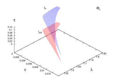
Figure 11: Variation of $\tau$ on ${\cal E}$ and $\lambda$ for multi-transonic shocked accretion in the Paczyński & Wiita (1980) potential $\Phi_{1}$. The red surface in the figure corresponds to the variation of $\tau$ with $\left[{\cal E},\lambda\right]$ for the outer acoustic horizons and the blue surface corresponds to the variation of $\tau$ with $\left[{\cal E},\lambda\right]$ for the inner acoustic horizons. This figure has been reproduced from Bilić, Das & Roy (2007)

It is now easy to calculate the analogue temperature for isothermal axisymmetric accretion in pseudo-Schwarzschild potential. Since $c_{s}$ is a function of the bulk temperature of the flow $T$, and since for isothermal accretion $T$ is constant throughout, the space derivative of the acoustic velocity $(dc_{s}/dr)$ is identically zero everywhere for any potential $\Phi_{i}$. Hence the expression for the analogue temperature can be obtained by setting $(dc_{s}/dr)=0$ in (179). The dependence of $T_{AH}$ on $\left[T,\lambda\right]$ has been discussed in Bilić, Das & Roy (2007) in detail.

XVII Epilogue

The primary motivation of this review article is to demonstrate the following:

One can propose that the general relativistic as well as the Newtonian/post-Newtonian accretion flow around an astrophysical black hole can be considered as an example of classical analogue gravity model realized in nature. To accomplish this task, one first formulates and solves the equations describing the accretion processes around black holes, and then provides the arguments that such accretion is transonic in general and the accreting material must encounter a sonic point at some specific length scale determined by various accretion parameters. The collection of such sonic points forms a null hypersurface, generators of which are the acoustic null geodesics, i.e. the phonon trajectories. Such a surface can be shown to be identical with an acoustic event horizon. The acoustic surface gravity and the corresponding analogue horizon temperature $T_{AH}$ at the acoustic horizon are then computed in terms of fundamental accretion parameters. Physically, the analogue temperature is associated with the thermal phonon radiation analogous to the Hawking radiation of the black-hole horizon. Acoustic white holes can also be generated if the accretion flow is multi-transonic and if such multi-transonic black-hole accretion encounters a stable shock. Such a white hole, produced at the shock, is always flanked by two acoustic black holes generated at the inner and the outer sonic points.

At this point one might as a crucial question: Does the accretion processes only around a black hole represents an analogue system, or any kind of astrophysical accretion exhibits the analogue gravity phenomena in general? From the discussions presented in this article, one understands that two of the essential requirements for a physical system to manifest the classical analogue gravity effects are the following:

1. The system should consists of transonic, barotropic fluid, and the fluid should, preferably, be inviscid in order not to violate the Lorentzian invariance.

2. An acoustic perturbation (or equivalent perturbation, a surface gravity wave for example, see, e.g., Sch$\ddot{\rm u}$tzhold & Unruh 2002) should propagate within such fluid for which a space time metric can be constructed. Such metric should incorporate a singularity (not always in a formal sense though), from which one can come up with the notion of the acoustic horizon.

Hence, it is obvious that hydrodynamic, non-dissipative accretion onto any astrophysical object should manifest the analogue gravity phenomena, if such accretion exhibits transonic properties, and if such accreting fluid configuration possesses a specific well defined symmetry (spherically symmetric or axisymmetric flow, for example). Hence, hydrodynamic, transonic, astrophysical accretion possessing a suitable symmetric geometrical configuration may exhibit the analogue properties in general, where the accretor resembles the sink.

Transonic accretion in astrophysics can be conceived to constitute an extremely important class of classical analogue gravity model. Among all the classical analogue systems studied in the literature so far, only an accreting astrophysical object incorporates gravity (through the general body force term in the Euler’s equation, even if the accretion is studied within the framework of the Newtonian space-time) in the analogue model. Also, the simplest possible analogue model may be constructed for such objects. For example, the spherically symmetric accretion of isothermal fluid onto a Newtonian/semi-Newtonian gravitating mass constitutes an analogue system which can be completely determined using a single parameter, the bulk flow temperature of the infalling material (see section 15.3).

However, among all the accreting astrophysical systems capable of manifesting the classical analogue effect, black hole accretion process deserves a very special status. The accreting astrophysical black holes are the only real physical candidates for which both the black-hole event horizon and the analogue sonic horizon may co-exist. Hence, the application of the analogue Hawking effect to the theory of transonic black hole accretion will be useful to compare the properties of these two types of horizons.

Recently, the spacetime geometry on the equatorial slice through a Kerr black hole has been shown to be equivalent to the geometry experienced by phonons in a rotating fluid vortex (Visser & Weinfurtner 2005). Since many astrophysical black holes are expected to possess non-zero spin (the Kerr parameter $a$), a clear understanding of the influence of spin on analogue models will be of great importance. Some important features on the dependence of the analogue temperature on the black hole spin angular momentum of an astrophysical black hole has been discussed in this article. In section 13.9 (Fig. 7 and related discussions), it has been shown that the black hole spin does influence the analogue gravity effect in a rotating relativistic fluid around it. Also the spin (of the black hole) - angular momentum (of the accreting material) coupling modulates such effect. Analogue effect is more prominent for retrograde (counter-rotating) flow, resulting a higher value of the corresponding analogue temperature.

In connection to the acoustic geometry, one can define an ‘anti-trapped surface’ to be a hypersurface in which the fluid flow will be outward directed with the normal component of the three-velocity greater than the local speed of sound. In stationary geometry, an anti-trapped surface will naturally be constructed by the collection of sonic points corresponding to a spherically symmetric or axisymmetric transonic wind solution emanating out from an astrophysical source. Transonic outflow (wind) is ubiquitous in astrophysics, spanning a wide range from solar/stellar winds to large-scale outflows from active galaxies, quasars, galactic micro-quasars and energetic gamma ray bursts (GRB). In section 13.7, it has been shown how to identify the critical and the sonic points corresponding to the wind solutions. Such a scheme can be useful in studying the transonic properties of outflow from astrophysical sources. Hence the formalism presented in this paper can be applied to study the analogue effects in transonic winds as well. Recently Kinoshita, Sendouda & Takahashi (2004) performed the causality analysis of the spherical GRB outflow using the concept of effective acoustic geometry. Such an investigation can be extended into a more robust form by incorporating the kind of work presented in this article, to study the causal structure of the transonic GRB outflows in axisymmetry, i.e. for energetic directed outflow originating from a black-hole accretion disc system progenitor.

In connection to the study of accreting black hole system as a classical analogue gravity model, so far the analogy has been applied to describe the classical perturbation of the fluid in terms of a field satisfying the wave equation in an effective geometry. Such works do not aim to provide a formulation by which the phonon field generated in this system could be quantized. To accomplish this task, one would need to show that the effective action for the acoustic perturbation is equivalent to a field theoretical action in curved space, and the corresponding commutation and dispersion relations should directly follow (see, e.g., Unruh & Sch$\ddot{\rm u}$tzhold 2003). Such considerations are beyond the scope of this article.

While describing the accretion disc dynamics, the viscous transport of the angular momentum is not explicitly taken into account. Viscosity, however, is quite a subtle issue in studying the analogue effects for disc accretion. Even thirty three years after the discovery of standard accretion disc theory (Shakura & Sunyaev, 1973; Novikov & Thorne 1973), exact modeling of viscous transonic black-hole accretion, including proper heating and cooling mechanisms, is still quite an arduous task, even for a Newtonian flow, let alone for general relativistic accretion. On the other hand, from the analogue model point of view, viscosity is likely to destroy Lorenz invariance, and hence the assumptions behind building up an analogue model may not be quite consistent. Nevertheless, extremely large radial velocity close to the black hole implies $\tau_{inf}\ll\tau_{visc}$, where $\tau_{inf}$ and $\tau_{visc}$ are the infall and the viscous time scales, respectively. Large radial velocities even at larger distances are due to the fact that the angular momentum content of the accreting fluid is relatively low (Beloborodov & Illarionov 1991; Igumenshchev & Beloborodov 1997; Proga & Begelman 2003). Hence, the assumption of inviscid flow is not unjustified from an astrophysical point of view. However, one of the most significant effects of the introduction of viscosity would be the reduction of the angular momentum. It has been observed that the location of the sonic points anti-correlates with $\lambda$, i.e. weakly rotating flow makes the dynamical velocity gradient steeper, which indicates that for viscous flow the acoustic horizons will be pushed further out and the flow would become supersonic at a larger distance for the same set of other initial boundary conditions.

In section 13.2, while constructing the geometry of the general relativistic accretion disc, the expression for the disc height has been derived using the prescription of Abramowicz, Lanza & Percival (1997). However, a number of other models for the disc height exist in the literature (Novikov & Thorne 1973; Riffert & Herold 1995; Pariev 1996; Peitz & Appl 1997; Lasota & Abramowicz 1997) The use of any other disc height model would not alter our conclusion that black-hole accretion disc solutions form an important class of analogue gravity models (see, e.g., Das 2004 for further details about the investigation of the relativistic disc dynamics using the disc height proposed by Lasota & Abramowicz (1997)). However, the numerical values of $T_{AH}$ and other related quantities would be different for different disc heights.

For all types of accretion discussed here, the analogue temperature $T_{\rm AH}$ is many orders of magnitude lower compared with the fluid temperature of accreting matter. However, the study of analogue effects may be measurably significant for accretion onto primordial black holes because the analogue as well as the actual Hawking temperature may be considerably high for such situations. There may be a possibility that intense Hawking radiation may not allow any accretion due to the domination of strong radiation pressure. However, the situation may be completely different for Randall-Sundrum type II cosmology, where during the high energy regime of braneworld cosmology, accretion may have significant effects on increasing the mass of the primordial black holes (Guedens, Clancy & Liddle 2002; Guedens, Clancy & Liddle 2002a; Majumdar 2003). In braneworld scenario, the accretion onto the primordial black holes from surrounding radiation bath may completely dominate over the evaporation process as long as radiation dominations persists. It would be interesting to investigate the analogue effects in primordial black hole accretion in Randall-Sundrum type - II cosmology, to study whether analogue radiation can really dominate over the accretion phase, resulting the enhancement of the black hole evaporation process. One may also like to investigate whether the first ‘black hole explosions’ due to Hawking radiation would be acoustic-mediated explosions of the medium surrounding the primordial black holes.

In recent years, considerable attention has been focused on the study of gravitational collapse of massive matter clump, in particular, on the investigation of the final fate of such collapse (for a review see, e.g., Krolak 1999). Goswami and Joshi (2004) have studied the role of the equation of state and initial data in determining the final fate of the continual spherical collapse of barotropic fluid in terms of naked singularities and the black-hole formation. It is tempting to study the analogue effects in such a collapse model. Since at some stage the velocity of the collapsing fluid will exceed the velocity of local acoustic perturbation one might encounter a sonic horizons at the radial locations of the corresponding transonic points in a stationary configuration. One should, however, be careful about the issue that many results in analogue models are based on the assumption of a stationary flow, whereas a collapse scenario is a full time dependent dynamical process.

The correspondence between general relativity and analogue gravity has so far been exploited only on a kinematical, i.e. geometrical level. The analogue gravity systems lack a proper dynamical scheme, such as Einstein’s field equations in general relativity and hence the analogy is not complete. A certain progress in this direction has recently been made by Cadoni and Mignemi (Cadoni 2005; Cadoni & Mignemi 2005), who have established a dynamical correspondence between analogue and dilaton gravity in 1+1 dimensions. We believe that the approach presented in this article in which an arbitrary background geometry serves as a source for fluid dynamics may shed a new light towards a full analogy between general relativity and analogue gravity.

References

- (1) Abraham, H., Bilić, N., & Das, T. K., 2006, Class. Quant. Grav. 23, 2371
- (2) Abramowicz, M. A., Czerny, B., Lasota, J. P., & Szuzkiewicz, E., 1988, ApJ. 332, 644.
- (3) Abramowicz, M. A., et al. (eds.) 1998, Theory of Black Hole Accretion Disks. Cambridge University Press.
- (4) Abramowicz, M. A., Lanza, A., & Percival, M. J. 1997, ApJ, 479, 179.
- (5) Anderson, M. 1989, MNRAS, 239, 19.
- (6) Armitage, P. J., Reynolds, C. S., & Chiang, J., 2001, APJ, 648, 868.
- (7) Artemova, I. V., Björnsson, G., & Novikov, I. D. 1996, ApJ, 461, 565
- (8) Babul, A., Ostriker, J. P., & Mészáros, P. 1989, ApJ, 347, 59.
- (9) Balbus, S. A., & Hawley, J. F., 1998, Reviews of Modern Physics, Volume 70, Issue 1, Pg. 1.
- (10) Barai, P., & Das, T. K., 2007, Does black hole spin influence the analogue effect? (In preparation).
- (11) Barai P, Das T K, Witta P J, 2004, Astrophys. J. Lett., 613, L49.
- (12) Barcelo, C., Liberati, S., and Visser, M., 2005, ‘Analogue Gravity’, Living Reviews in Relativity, Vol. 8, no. 12, websource http://relativity.livingreviews.org/Articles/lrr-2005-12/, also at gr-qc/0505065
- (13) Barceló, C, Liberati, S., Sonego, S., & Visser, M, 2004, New J. Phys. 6, 186, gr-qc/0408022.
- (14) Barcelo C, Liberati S, Visser M, 2003, Int. Jour. Mod. Phys, D., 12, 1641.
- (15) Bardeen J M, Carter B, Hawkings S W, 1973, Commun. Math. Phys., 31 1641.
- (16) Bardeen, J. M., & Petterson, J. A. 1975, ApJ, 195, L65.
- (17) Basak, S., 2005, Analog of Superradiance effect in BEC, gr-qc/0501097.
- (18) Basak, S. & Majumdar, P., 2003, Class. Quant. Grav., 20, 2929.
- (19) Begelman M C, 1978, Astron. Astrophys., 70, 583.
- (20) Beloborodov, A. M., & Illarionov, A. F. 1991, MNRAS, 323, 167.
- (21) Bekenstein J D, 1972a, Phys. Rev. D., 5, 2403.
- (22) Bekenstein J D, 1972, Phys. Rev. D., 5, 1239.
- (23) Bekenstein J D, 1973, Phys. Rev. D., 7, 2333.
- (24) Bekenstein J D, 1975, Phys. Rev. D., 12, 3077.
- (25) Bekenstein J D, 1980, Physics Today, January, 24.
- (26) Berti E, Cardoso V, Lemos J P, 2004, Physical Review D., 70, Issue 12, id. 124006.
- (27) Bili, N. 1999, Class. Quant. Grav. 16, 3953
- (28) Bili, N., Das, T. K., & Roy, S., 2007, Pseudo-Schwarzschild shocked accretion disc as an analogue gravity model, (In preperation).
- (29) Birrell, N. D., & Davies, P. C. W. 1982, Quantum fields in curved space, Cambridge University Press, Cambridge.
- (30) Bisikalo, A. A., Boyarchuk, V. M., Chechetkin, V. M., Kuznetsov, O. A., & Molteni, D. 1998, MNRAS, 300, 39.
- (31) Bisnovatyi-Kogan, G., 1998, in Observational Evidence For Black Holes in the Universe, ed. S. K. Chakrabarti (Dordrecht: Kluwer).
- (32) Bisnovatyi-Kogan, G. S., Zel’Dovich, Ya. B, & Syunyaev, R. A. 1971, Soviet Astronomy, 15, 17.
- (33) Blandford, R. D., 1999, in Astrophysical Discs. ASP Conference Series.
- (34) Blondin, J. M., & Ellison, D. C. 2001, ApJ, 560, 244.
- (35) Blondin, J. M., & Konigl, A. 1987, ApJ, 323, 451.
- (36) Blumenthal, G R, Mathews W G, 1976, Astrophys. J., 203, 714.
- (37) Bondi, H. 1952, MNRAS, 112, 195
- (38) Boyer, R. H., & Lindquist, R. W. 1967, J. Math. Phys. 8, 265.
- (39) Brevik I, Halnes G, 2002, Phys. Rev. D, 65, 024005.
- (40) Brinkmann W, 1980, Astron. Astrophys., 85, 146.
- (41) Brown J D, 1995, Phys. Rev. D., 47, 1420.
- (42) Caditz, D. M., & Tsuruta, S. 1998, ApJ, 501, 242.
- (43) Cadoni, M., 2005, Class. Quant. Grav. 22, 409
- (44) Cadoni, M., & Mignemi, S., 2005, Acoustic analogues of black hole singularities, Phys. Rev. D 72, 084012, gr-qc/0504143.
- (45) Cardoso, V., 2005, Acoustic black holes, physics/0503042
- (46) Cardoso, V, Lemos J P S, Yoshida S, 2004, Quasinormal modes and stability of the rotating acoustic black hole: numerical analysis, gr-qc/0410107.
- (47) Carter, B., 1971, Phys. Rev. Lett., 26, 331.
- (48) Chakrabarti, S. K. 1989, ApJ, 347, 365.
- (49) Chakrabarti, S. K. 1990, ApJ, 350, 275.
- (50) Chakrabarti, S. K. 1996, ApJ, 471, 237.
- (51) Chakrabarti, S. K. 1996a, MNRAS, 283, 325.
- (52) Chakrabarti, S. K. 1996b, ApJ, 471, 237.
- (53) Chakrabarti, S. K. 1996c, Physics Reports, 266, 229.
- (54) Chakrabarti, S. & Das, S., 2004, MNRAS, 349, 649.
- (55) Chang, K. M., & Ostriker, J. P. 1985, ApJ, 288, 428.
- (56) Chaudhury, S., Ray, A. K., & Das, T. K., 2006, Critical properties and stability of stationary solutions in multi-transonic pseudo-Schwarzschild accretion, Monthly Notices of the Royal Astronomical Society, 373, 146, also at arXiv:astro-ph/0607451.
- (57) Chen, X., & Taam, R. E., 1993, APJ, 412, 254.
- (58) Cherubini, C., Federici, F., & Succi, S., 2005, Phys. Rev. D., 72, 084016.
- (59) Choy, K., Kruk, T., Carrington, M. E., Fugleberg, T., Zahn, J., Kobes, R., Kunstatter, G., & Pickering, D., 2005, Energy Flow in Acoustic Black Holes, (gr-qc/0505163).
- (60) Contopoulos, J., & Kazanas, D. 1995, ApJ, 441, 521.
- (61) Corley, S., & Jacobson, T. 1996, Phys. Rev. D 54, 1568.
- (62) Dasgupta, S., Bili, N., and Das, T. K., 2005, General Relativity & Gravitation (GRG), Volume 37, Number 11, 1877-1890.
- (63) Das, T. K., 2001, A & A, 376, 697.
- (64) Das, T. K., 2002, ApJ, 577, 880.
- (65) Das T K, 2002, MNRAS, 330, 563.
- (66) Das T K, 2003, ApJ, Volume 588, Issue 2, pp. L89-L92.
- (67) Das, T. K. 2004, MNRAS, 375, 384.
- (68) Das, T. K. 2004a, Classical & Quantum Gravity, 21, 5253.
- (69) Das, T. K., Bili, N., & Dasgupta, S., 2006, Black-Hole Accretion Disc as an Analogue Gravity Model, arXiv:astro-ph/0604477.
- (70) Das, T. K., Pendharkar, J. K., & Mitra, S. 2003, ApJ, 592, 1078.
- (71) Das T K, Sarkar A, 2001, Astron. Astrophys., 374, 1150.
- (72) Das, T. K., & Chakrabarti, S. K. 1999, Class. Quantum Grav. 16, 3879
- (73) Das, T. K., Rao, A. R., & Vadawale, S. R. 2003, MNRAS, 343, 443
- (74) de Lorenci V A, Klippert R, Obukhov Y N, 2003, Phys. Rev. D., 68, 061502.
- (75) Demianski, M., & Ivanov, P. B. 1997, A & A, 324, 829.
- (76) Federici, F., Cherubini, C., Succi, S., & Tosi, M. P., 2005, Superradiance from BEC vortices: a numerical study, gr-qc/0503089.
- (77) Foglizzo, T. 2001, A & A, 368, 311.
- (78) Foglizzo, T., & Tagger, M. 2000, A & A, 363, 174.
- (79) Fragile, P. C., & Anninos, P., 2005, ApJ, 623, 347.
- (80) Frank J, King A R, Raine D J, 1992, Accretion Power in Astrophysics, Cambridge: Cambridge Univ. Press.
- (81) Fukue, J. 1983, PASJ, 35, 355.
- (82) Fukue, J. 1987, PASJ, 39, 309.
- (83) Fukumura, K., & Tsuruta, S., 2004, ApJ, 611, 964.
- (84) Garay L J, Anglin J R, Cirac J I, Zoller P, 2000, Phys. Rev. Lett., 85, 4643.
- (85) Garay L J, Anglin J R, Cirac J I, Zoller P, 2001, Phys. Rev. A., 63, 023611.
- (86) Goswami, S., Khan, S. N., Ray, A. K., & Das, T. K., 2007, Axisymmetric black hole accretion in the Kerr metric as an autonomous dynamical system, to appear in the Monthly Notices of the Royal Astronomical Society, arXiv:astro-ph/0702733.
- (87) Goswami, R., & Joshi, P., 2004, Class. Quant. Grav. 21, 3645.
- (88) Guedens, R., Clancy, D., & Liddle, A. R., 2002, Phys. Rev. D., vol. vol. 66, Issue 8, id. 083509.
- (89) Guedens, R., Clancy, D., & Liddle, A. R., 2002a, Phys. Rev. D., vol. 66, Issue 4, id. 043513.
- (90) Guessoum, N., & Kazanas, D. 1999, ApJ, 512, 332.
- (91) Gullstrand, A., 1922, Allegemeine Isung des statischen einkrper-problems in der Einsteinshen gravitations theorie, Arkiv. Mat. Astron. Fys., 16(8), 1.
- (92) Haiman, Z.& Quataert, E., 2004, The Formation and Evolution of the First Massive Black Holes, in ‘Supermassive Black Holes in the Distant Universe’, ed. Barger, A. J., Astrophysics and Space Science Library Volume 308, Kluwer Academic Publishers, Dordrecht, The Netherlands, p. 147.
- (93) Hawkings S W, 1975, Commun. Math. Phys., 43, 199.
- (94) Hawley, J. F., & Krolik, J. H., 2001, APJ, 548, 348.
- (95) Hawley, J. F., Wilson, J. R., & Smarr, L. L. 1984, ApJ, 277, 296.
- (96) Helfer A D, 2003, Rept. Prog.Phys., 66, 943.
- (97) Heusler M, 1996, Black Hole Uniqueness Theorem. Cambridge University Press, Cambridge.
- (98) Ho, L. C. 1999, in Observational Evidence For Black Holes in the Universe, ed. S. K. Chakrabarti (Dordrecht: Kluwer), 153
- (99) Hoshi, R., & Shibazaki, N., 1977, Prog. Theor. Phys. 7, 203.
- (100) Hoyle F, Lyttleton R A, 1939, Proc. Camb. Phil. Soc., 35, 59.
- (101) Hughes, S. A., 2005, Trust but verify: The case for astrophysical black holes, SLAC Summer Institute Lectures, hep-ph/0511217.
- (102) Ichimaru, S., 1977, ApJ. 214, 840.
- (103) Igumenshchev, I. V., & Beloborodov, A. M., 1997, MNRAS, 284, 767.
- (104) Igumenshchev, I. V. & Abramowicz, M. A. 1999, MNRAS, 303, 309.
- (105) Illarionov, A. F. 1988, Soviet Astron., 31, 618.
- (106) Illarionov, A. F., & Sunyaev, R. A. 1975, A & A, 39, 205.
- (107) Israel W, 1976, Phys. Lett., 57A, 107.
- (108) Israel W, 1967, Phys. Rev., 164, 1776.
- (109) Jacobson, T. 1991a, Phis. Rev. D 44, 1731.
- (110) Jacobson, T. 1992, Phys. Rev. D 48, 728.
- (111) Jacobson, T. A. 1991, Phys. Rev. D. 44, 1731
- (112) Jacobson, T. A. 1999, Prog. Theor. Phys. Suppl. 136, 1
- (113) Jacobson, T. A, Volovik G E, 1998, Phys. Rev. D., 58, 064021.
- (114) Jacobson, T. A., & Parentani, R., 2005, An ECHO of Black Holes, Scientific American, December issue, Page 48.
- (115) Jordan, D. W., & Smith, P., 2005, Non Linear Ordinary Differential Equations, Oxfod University Press, Third edition, 2005 Paperback, ISBN 0198565623.
- (116) Jones, F. C., & Ellison, D. C. 1991, Space Science Review, 58, 259.
- (117) Kafatos, M.& Yang, R. X. 1994, A & A, 268, 925.
- (118) Kato, S., Fukue, J., & Mineshige, S., 1998, Black Hole Accretion Disc, Kyoto University Press.
- (119) Kazanas, D., & Ellison, D. C. 1986, ApJ, 304, 178.
- (120) Keifer C, 1998, Black Hole: Theory and observation eds. Hehl F W, Keifer C, Metzler R, Springer, Berlin, (also gr-qc/9803049).
- (121) Kerr, R. P., 1963, Phys. Rev. Lett., 11, 237.
- (122) Kim, W. T., Son, E. J., & Yoon, M. S., 2005, Statistical entropy and superradiance in 2+1 dimensional acoustic black holes, gr-qc/0504127.
- (123) Kinoshita, S., Sendouda, Y., & Takahashi, K., 2004, Phys. Rev. D., 70, 123006.
- (124) Krolak, A., 1999, Progress of Theoretical Physics Supplement, 136, 45.
- (125) Kovalenko I. G., & Eremin, M. A. 1998, MNRAS, 298, 861.
- (126) Kraft, R., 1963, in Advances in Astron. & Astrophys. ed. Kopal, Z. 2, 43.
- (127) Kumar, S., 1988, MNRAS, 233, 33.
- (128) Lai, D., & Goldreich, P. 2000, ApJ, 535, L402.
- (129) Landau, L. D., & Lifshitz, E. D. 1959, Fluid Mechanics, New York: Pergamon
- (130) Lanza, A., 1992, ApJ, 389, 141.
- (131) Lasota, J. P., & Abramowicz, M. A. 1997, Class. Quantum Grav. 14, A237.
- (132) Lemaître, G., 1933, L’universe en expansion, Ann. Soc. Sci. (Bruxelles), A 53, 51.
- (133) Lense, J., & Thirring, H. 1918, Phys. Z., 19, 156.
- (134) Leonhardt W, 2002, Nature., 415, 406.
- (135) Leonhardt, W, 2003, Reports on Progress in Phys., 66, 1207
- (136) Lepe, S., & Saavedra, J., 2005, Phys. Lett. B 617, 174.
- (137) Liang, E. P. J., & Thompson, K. A., 1980, ApJ. 240, 271.
- (138) Liang, E. P. T., & Nolan, P. L. 1984, Space Sci. Rev., 38, 353.
- (139) Lin, D. N. C., & Papaloizou, J. C. B., 1996, ARA&A. 34. 703.
- (140) Lu, J. F., Yu, K. N., Yuan, F., & Young, E. C. M. 1997, A & A, 321, 665.
- (141) Lu, J. F., & Zhou, B. 2005, ApJ, 635, L17.
- (142) Maccarone, T. J., 2002, MNRAS, 336, 1371.
- (143) Majumdar, A. S., 2003, Physical Review Letters, vol. 90, Issue 3, id. 031303.
- (144) Malec E, 1999, Phys. Rev. D., 60, 104043.
- (145) Mandal, I., Ray, A. K., & Das T. K., 2007, ‘Critical properties of spherically symmetric black hole accretion in Schwarzschild geometry’, arXiv:astro-ph/0702733.
- (146) Manmoto, T. 2000, ApJ, 534, 734.
- (147) Markoff, S., Melia, F., & Falcke, H. 1999, ApJ, 522, 870.
- (148) Matsumoto, R., Kato. S., Fukue. J., & Okazaki. A. T., 1984, PASJ, 36, 71.
- (149) Mészáros, P. & Ostriker, J. P., 1983, ApJ, 273, L59.
- (150) Michel F C, 1972, Astrophys. Space Sci., 15, 153.
- (151) Misner, C. W., Thorne, K. S., & Wheeler, J. A., 1973, Gravitation (San Francisco, CA: Freeman)
- (152) Molteni, D., Sponholz, H., & Chakrabarti, S. K., 1996, ApJ, 457, 805.
- (153) Moncrief V, 1980, Astrophys. J., 235, 1038.
- (154) Moscibrodzka, M., Das, T. K., & Czerny, B. 2006, MNRAS, 370, 219.
- (155) Muchotrzeb, B., 1983, Acta Astron. 33, 79.
- (156) Muchotrzeb, B., & Paczyński, B., 1982, Acta. Astron. 32, 1.
- (157) Narayan, R., Kato, S., & Honma, F., 1997, APJ, 476, 49.
- (158) Narayan, R., & Yi, I., 1994, ApJ. 428, L13.
- (159) Nelson, R. P., & Papaloizou, J. C., 2000, MNRAS, 315, 570.
- (160) Newman, E. T., Couch, R., Chinnapared, K., Exton, A., Prakash, A., & Torrence, R., 1965, J. Math. Phys., 6, 918.
- (161) Nordstrm, G., 1918, On the energy of the gravitational field in Einstein’s theory, Proc. K. Ned. Akad. Wetensch., 20, 1238-1245.
- (162) Novello M, Perez Bergliaffa S, Salim J, DeLorenci V A, Klippert R, 2003, Class. Quant. Grav., 20, 859.
- (163) Novello, M., Visser, M., & Volovik, G., 2002, (ed) Artificial Black Holes, World Scientific, Singapore.
- (164) Novikov, I., & Thorne, K. S., 1973, in Black Holes. ed. DeWitt, C. & DeWitt, B. Gordon & Breach. NY. p. 343.
- (165) Nowak, A. M., & Wagoner, R. V. 1991, ApJ, 378, 656.
- (166) Paczyński, B., & Bisnovatyi-Kogan, G., 1981, Acta Astron. 31, 283.
- (167) Paczynśki, B., & Wiita, P. J., 1980, A & A, 88, 23.
- (168) Padmanabhan, T., 2005, Physics Reports, 406, 49.
- (169) Page D N, 2004, Hawking Radiation and Black Hole Thermodynamics, (hep-th/0409024)
- (170) Painlevé, P., 1921, La mécanique classique et la theorie de la relativité, C. R. Acad. Sci. (Paris) 173, 677.
- (171) Parentani R, 2002, Int. Jour. Mod. Phys. A., 17, 2721.
- (172) Pariev, V. I. 1996, MNRAS, 283, 1264.
- (173) Park, M. G. 1990a, ApJ, 354, 83.
- (174) Park, M. G. 1990, ApJ, 354, 64.
- (175) Parker, E. N., 1965, Space Science Reviews, vol. 4, p.666.
- (176) Peitz, J. & Appl, S. 1997, MNRAS, 286, 681.
- (177) Petterson, J. A., 1977, ApJ, 214, 550.
- (178) Prendergast, K. H., & Burbidge, G. R., 1968, ApJ. 151, L83.
- (179) Price, R., 1972, Phys. Rev. D5, 2419, 2439.
- (180) Pringle, J. E., 1981, Annual review of astronomy and astrophysics. Volume 19, Pg. 137.
- (181) Proga, D., & Begelman, M. C., 2003, ApJ, 582, 69.
- (182) Protheroe, R. J., & Kazanas, D. 1983, ApJ, 256, 620.
- (183) Protheroe, R. J., & Szabo, A. P. 1992, Physical Review Letters, 69, 2885.
- (184) Ray, A. K., & Bhattacharjee, J. K., 2002, Phys. Rev. E., vol. 66, Issue 6, id. 066303.
- (185) Rees, M. J., 1984, Annual review of astronomy and astrophysics, Volume 22, p. 471.
- (186) Rees, M. J., 1997, in Black Holes & Relativity: Chandrasekhar Memorial Conference. ed. Wald, R.
- (187) Rees M J, 2002, Lighthouses of the Universe: The Most Luminous Celestial Objects and Their Use for Cosmology, Proceedings of the MPA/ESO/, p. 345.
- (188) Reissner, H., 1916, ber die Eigengravitation des elektrischen Feldes nach der Einsteinschen Theorie, Ann. Phys. (Berlin), 59, 106-120.
- (189) Reznik B, 2000, Phys. Rev. D., 62, 044044.
- (190) Riffert, H., & Herold, H. 1995, ApJ, 450, 508.
- (191) Robinson, E. L., 1976, ARA&A. 14, 119.
- (192) Robinson, D. C., 1975, Phys. Rev. Lett., 34, 905.
- (193) Sawada, K., Matsuda, T., & Hachisu, I., 1986, MNRAS, 221, 679.
- (194) Schtzhold, R, Gnter, P, Gerhard S, 2002, Phys. Rev.Lett., 88, 061101.
- (195) Schtzhold, R, Unruh W G, 2002, Phys. Rev. D., 66, 044019.
- (196) Scheuer, P. A., & Feiler, R., 1996, MNRAS, 282, 291.
- (197) Schwarzschild, K., 1916, Sitzungsberichte der Deutschen Akademie der Wissenschaften zu Berlin, Klasse fr Mathematik, Physik, und Technik, 189.
- (198) Shakura, N. I., & Sunyaev, R. A., 1973, A & A. 19, 137.
- (199) Shapiro S, 1973a, Astrophys. J., 185, 69.
- (200) Shapiro S, 1973, Astrophys. J., 180, 531.
- (201) Shvartsman, V. F., 1971a, Soviet. Astr. 15, 377.
- (202) Shvartsman, V. F., 1971, Soviet. Astr. 14, 662.
- (203) Slatyer, T. R., & Savage, C. M., 2005, Class. Quantum Grav. 22, 3833.
- (204) Spruit, H. C. 1987, A & A, 184, 173.
- (205) Takahashi, M., Rilett, D., Fukumura, K., & Tsuruta, S., 1992, ApJ, 572, 950.
- (206) Tóth, G., Keppens, R., & Botchev, M. A. 1998, A & A, 332. 1159.
- (207) Unruh, W. G. 1981, Phys. Rev. Lett. 46, 1351
- (208) Unruh, W. G. 1995, Phys. Rev. D. 51, 2827
- (209) Unruh, W. G. & Schtzhold, R. 2003, Phys. Rev. D. 68, 024008
- (210) Visser, M. 1998, Class. Quant. Grav. 15, 1767
- (211) Visser, M. & Weinfurtner, S., 2005, Class. Quant. Grav. 22, 2493.
- (212) Volonteri, M., 2006, Evolution of supermassive black holes, eprint arXiv:astro-ph/0602630.
- (213) Volovik G E, 1999, Proc. Natl. Acad. Sci., USA 96, 6043 (also cond-mat/9812381).
- (214) Volovik G E, 2000, gr-qc/0004049.
- (215) Volovik G E, 2001, Physics Reports., 351, 195.
- (216) Wald R M, 1984, General relativity. Chicago, University of Chicago Press.
- (217) Wald R M, 1994, Quantum Field Theory in Curved Spacetime and Black Hole Thermodynamics, Chicago University Press.
- (218) Wald R M, 2001, Living Rev Rel. 4, 6., http://physics.uchicago.edu/trel.htmlWald.
- (219) Weyl, H., “1919, ber die statischen kugelsymmetrischen Lsungen von Einsteins kosmologischen Gravitationsgleichungen, Phys. Z., 20, 31-34.
- (220) Wiita, P. J., 1982, ApJ. 256, 666.
- (221) Wiita, P. J., 1998, in Black Holes, Gravitational Radiation and the Universe, eds. B.R. Iyer & B. Bhawal p. 249. (Dordrecht: Kluwer).
- (222) Yang, R., & Kafatos, M. 1995, A & A, 295, 238.