ACS imaging of star clusters in M51

Abstract

Context. Size measurements of young star clusters are valuable tools to put constraints on the formation and early dynamical evolution of star clusters.

Aims. We use HST/ACS observations of the spiral galaxy M51 in F435W, F555W and F814W to select a large sample of star clusters with accurate effective radius measurements in an area covering the complete disc of M51. We present the dataset and study the radius distribution and relations between radius, colour, arm/interarm region, galactocentric distance, mass and age.

Methods. We select a sample of 7698 (F435W), 6846 (F555W) and 5024 (F814W) slightly resolved clusters and derive their effective radii ($R_{\mathrm{eff}}$) by fitting the spatial profiles with analytical models convolved with the point spread function. The radii of 1284 clusters are studied in detail.

Results. We find cluster radii between 0.5 and $\sim$10 pc, and one exceptionally large cluster candidate with $\mbox{$R_{\mathrm{eff}}$}=21.6$ pc. The median $R_{\mathrm{eff}}$ is 2.1 pc. We find 70 clusters in our sample which have colours consistent with being old GC candidates and we find 6 new “faint fuzzy” clusters in, or projected onto, the disc of M51. The radius distribution can not be fitted with a power law similar to the one for star-forming clouds. We find an increase in $R_{\mathrm{eff}}$ with colour as well as a higher fraction of clusters with $\mbox{$B\!-\!V$}\gtrsim 0.05$ in the interarm regions. We find a correlation between $R_{\mathrm{eff}}$ and galactocentric distance ($R_{\mathrm{G}}$) of the form $\mbox{$R_{\mathrm{eff}}$}\propto R_{\mathrm{G}}^{0.12\pm 0.02}$, which is considerably weaker than the observed correlation for old Milky Way GCs. We find weak relations between cluster luminosity and radius: $\mbox{$R_{\mathrm{eff}}$}\propto L^{0.15\pm 0.02}$ for the interarm regions and $\mbox{$R_{\mathrm{eff}}$}\propto L^{-0.11\pm 0.01}$ for the spiral arm regions, but we do not observe a correlation between cluster mass and radius.

Conclusions. The observed radius distribution indicates that shortly after the formation of the clusters from a fractal gas, the radii of the clusters have changed in a non-uniform way. We find tentative evidence suggesting that clusters in spiral arms are more compact.

1 Introduction

One of the most striking questions related to star cluster formation concerns the transition from the densest parts of the star-forming Giant Molecular Clouds (GMCs) to the clusters that emerge from them. Observations show that the masses and radii of clouds follow a clear relation of the form $R_{\mathrm{GMC}}\propto M_{\mathrm{GMC}}^{1/2}$ (e.g. Larson 1981; Solomon et al. 1987) down to the scale of the star forming clumps (Williams et al. 1995). Such a relation is expected for self-gravitating clouds, which are in virial equilibrium and pressure bounded by their surroundings (e.g. Elmegreen 1989). The same mass-radius relation is observed for complexes of multiple clusters (Elmegreen & Salzer 1999; Elmegreen et al. 2001; Bastian et al. 2005a). Elliptical galaxies and very massive ($>10^{6.5}\leavevmode\nobreak\ \mbox{$\mathrm{M_{\odot}}$}$) stellar clusters follow a similar relation ($R\propto M^{0.62}$ (Haşegan et al. 2005)), which advocates a possibility of forming very massive clusters by merging of low mass clusters (Fellhauer & Kroupa 2005; Kissler-Patig et al. 2006).

However, for individual star clusters that emerge from the star forming clouds/clumps, a relation between mass and radius is not present (Van den Bergh et al. 1991; Bastian et al. 2005b; Jordán et al. 2005) or at least strongly weakened (Zepf et al. 1999; Hunter et al. 2003; Mackey & Gilmore 2003; Larsen 2004; Lee et al. 2005). Since this is already the case for very young clusters, it indicates that during, or shortly after ($<10$ Myr) the transition from clouds to clusters the mass and/or the radius of the objects change.

These changes in mass and/or radius are likely to be reflected in changes in the mass and radius distributions (Ashman & Zepf 2001). On the one hand, however, the mass distributions of both clouds and clusters show great similarities. Both can be approximated by power laws of the form $N(M)\mathrm{d}M\propto M^{-\alpha}\mathrm{d}M$, with the index $\alpha$ in the range of 1.5–2.0 (see Sanders et al. 1985; Solomon et al. 1987; Harris & Pudritz 1994; Brand & Wouterloot 1995; Elmegreen & Falgarone 1996; Fukui et al. 2001 for clouds and see e.g. Zhang & Fall 1999; Ashman & Zepf 2001; Bik et al. 2003; de Grijs et al. 2003; Hunter et al. 2003 for clusters). Recently, some studies have found evidence for an upper mass truncation of the cluster mass distribution Gieles et al. (2006a); Dowell et al. (2006), which is also found for the mass distributions of GMCs (Rosolowsky 2005). On the other hand, the radius distributions are less well constrained, especially for extra-galactic star clusters. If we approximate the radius distributions by a power law of the form $N(R)\mathrm{d}R\propto R^{-\eta}\mathrm{d}R$, the average value of the index for GMCs is observed to be $\eta=3.3\pm 0.3$ (Harris & Pudritz 1994; Elmegreen & Falgarone 1996), consistent with the gas having a fractal structure with a fractal dimension $\eta-1=2.3\pm 0.3$ (Mandelbrot 1983; Elmegreen & Elmegreen 2001). For young clusters in NGC 3256 Zepf et al. (1999) find $\eta\approx 3.4$, while Bastian et al. (2005, from now on referred to as “B05”) find $\eta=2.2\pm 0.2$ for star clusters in the disc of M51. This difference, however, seems to be caused by the erroneous addition of $+1$ to the index in the result of Ashman & Zepf (2001).

Our understanding of whether or not the mass and radius distribution of clouds and clusters are similar, and to which degree, is directly coupled to our understanding of star formation and the early evolution of star clusters. Besides that, possible explanations for the lack of a mass-radius relation for clusters which change the mass and/or the radius of the clusters in a non-uniform way, are likely to affect the mass and radius distributions (Ashman & Zepf 2001). It is therefore important to put better constraints on these distributions, and in this work we will focus on the radius distribution of young star clusters.

In the study presented here we exploit the superb resolution and large field-of-view of the new HST Advanced Camera for Surveys (ACS) observations of M51, taken as part of the Hubble Heritage Project. These observations allow us to measure the radii of a large sample of clusters in an area covering, for the first time, the complete disc of M51 and its companion, NGC 5195 at a $0.05\arcsec$ resolution. In this work, which is the first in a series of papers, we present the dataset and we study the radius distribution for the complete cluster sample and for cluster samples with a different background surface brightness (“background regions”). The differences in background regions are likely to reflect differences in environmental conditions, which could have an impact on the early evolution of star clusters.

The radii of star clusters in M51 have already been studied by B05 and Lee et al. (2005). However, these studies used lower resolution HST/WFPC2 data and were not covering the complete disc. Besides this, we use different selection criteria for the clusters than B05, based on the clusters actually being resolved and clearly separated from nearby contaminating sources. In combination with the larger field-of-view and the higher resolution of the ACS data, this leads to a larger sample of clusters, divided in different background regions.

The structure of this paper is as follows: in § 2 we describe the dataset, the selection of sources and background regions and the photometry. The radius measurements are described in § 3 and in § 4 we describe experiments with artificial clusters to determine the accuracy and detection limits of our methods. Our selection criteria and a description of our cluster sample are presented in § 5, followed by a comparison between ACS and WFPC2 data in § 6. The radius distribution is presented in § 7, and we search for correlations between mass, radius and galactocentric distance in § 8. In §9 we finish with the summary and conclusions.

2 Observations, source selection and photometry

2.1 Observations

We make use of the HST/ACS dataset of M51 (NGC 5194, a late type Sbc galaxy), taken as part of the Hubble Heritage Project in January 2005 (proposal ID 10452, PI: S. V. W. Beckwith). The dataset consists of 6 ACS pointings using the Wide Field Channel (WFC) in F435W ($\sim B$), F555W ($\sim V$), F814W ($\sim I$) and F658N ($\sim H\alpha$), with 4 dithered exposures per filter, as is summarized in Table 1. The observations were reduced and drizzled into one mosaic image by Mutchler et al. (2005). In summary, the standard ACS pipeline (CALACS) was used for bias, dark and flat-field corrections of the individual dithered images. The corrected images were then combined into one mosaic image using the MultiDrizzle task (Fruchter & Hook 2002; Koekemoer et al. 2002), which also corrects for filter-specific geometric distortion, cosmic rays and bad pixels. For a complete description of the dataset we refer to Mutchler et al. (2005) and the M51 mosaic website (http://archive.stsci.edu/prepds/m51/). For details on the standard pipeline processing we refer to the ACS Data Handbook (Pavlovsky et al. 2005).

The resulting mosaic image covers a region of $430\times 610\arcsec$ ($=17.5\times 24.8$ kpc) with a resolution of 2.0 pc per pixel, where we assumed a distance modulus of $m-M=29.62$ from Feldmeier et al. (1997), i.e. a distance of $8.4\pm 0.6$ Mpc. The covered region is large enough to include the complete spiral disc of M51, as well as its companion NGC 5195 (a dwarf barred spiral of early type SB0), while at the same time the resolution is good enough to resolve stellar cluster candidates, i.e. to distinguish them from stars by measuring their sizes and comparing these to the Point Spread Function (PSF) of the HST/ACS camera.

Table 1: Overview of the filters and exposure times used. The limiting magnitude is for a point source with S/N = 5.

Filter	Exposure time	Limiting magnitude
F435W	$4\times 680$ s = 2720 s	27.3 mB
F555W	$4\times 340$ s = 1360 s	26.5 mV
F814W	$4\times 340$ s = 1360 s	25.8 mI
F658N$+N$[II]	$4\times 680$ s = 2720 s	–

2.2 Source selection

For source selection we used the SExtractor package (Bertin & Arnouts 1996, version 2.3.2). SExtractor first generates a background map by computing the mean and standard deviation of every section of the image with a user defined grid size for which we choose $10\times 10$ pixels. In every section the local background histogram is clipped iteratively until every remaining pixel value is within $\pm 3\sigma$ of the median value. The mean of the clipped histogram is then taken as the local background value. Every area of at least three adjacent pixels that exceeded the background by at least $5\sigma$ was called a source. For details on the background estimation and the source selection we refer to the SExtractor user manual (Bertin & Arnouts 1996) or Holwerda (2005). The coordinates of the sources in F435W  F555W and F814W were matched and only sources that were detected in all three filters within two pixel uncertainty were kept. This resulted in a list of $75\,436$ sources, including cluster candidates but also many stars and background galaxies. We did not apply any selection criteria based on shape, sharpness or size during the source selection with SExtractor. However, in § 5 we use individual radii measurements to select a large sample of cluster candidates from the source list.

2.3 Background selection

In order to study any possible relations between radius and environment, and to perform completeness and accuracy tests for different background levels, we divided the image in three regions according to the background surface brightness. These background regions were selected by smoothing the F555W image with a boxcar average of 200 pixels. Consequently, pixels with a value $<0.19\leavevmode\nobreak\ \mathrm{e}^{-}/\mathrm{s}$ (corresponding to a surface brightness $\mu>21.02$ mag arcsec^-2) were flagged “low background”. Pixel values $\geq 0.19\leavevmode\nobreak\ \mathrm{e}^{-}/\mathrm{s}$ and $<0.25\leavevmode\nobreak\ \mathrm{e}^{-}/\mathrm{s}$ ($20.72<\mu<21.02$ mag arcsec^-2) were flagged “intermediate background” and pixels with a value $\geq 0.25\leavevmode\nobreak\ \mathrm{e}^{-}/\mathrm{s}$ ($\mu<20.72$ mag arcsec^-2) were flagged “high background”. These values were chosen because they resulted in a contour map, shown in Fig. 1, in which the high background region clearly follows most of the inner spiral arms, covering most areas that would be marked “high background” if the selection would take place by eye. The “intermediate” region should be considered as a transition region to clearly separate cluster samples within a low and high background region.

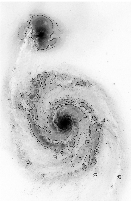
Figure 1: The contours outlining the three background regions, superimposed on the HST/ACS mosaic image in the F555W passband. The solid lines enclose “high background” regions, and everything outside the dashed lines indicates the “low background” regions. The regions in between solid and dashed lines are called “intermediate background”.

2.4 Point spread function

For our photometry, radius measurements and artificial cluster experiments we need a filter dependent PSF. Since there are not enough bright, isolated point sources in the M51 mosaic image to determine the PSF accurately, the PSF was observationally determined from a crowded star field on a drizzled image of the Galactic globular cluster 47 Tuc (NGC 104, HST proposal GO-9281, PI: J. E. Grindlay). For each filter a separate PSF was determined.

With drizzled data, the size of the PSF depends on the choice of the drizzle kernel and the accuracy with which the flux from multiple images is combined. We note that the image of 47 Tuc was drizzled in a slightly different way than the M51 image. The 47 Tuc images were drizzled using a square kernel with a size of one pixel (i.e. $\mathrm{pixfrac}=1.0$ (Fruchter & Hook 2002)), while a Gaussian kernel with $\mathrm{pixfrac}=0.9$ was used for M51. Therefore, we expect some differences between the PSFs, with the M51 PSF possibly being larger than the 47 Tuc PSF. This could lead to an overestimation of the measured radii. However, tests by Larsen (2004) have shown that the lower limit down to which Ishape can detect a source as being resolved is $\sim$10% of the FWHM of the PSF. At the distance of M51 and with a FWHM of the ACS PSF of $\sim$2.1 pixels, this corresponds to an effective radius ($R_{\mathrm{eff}}$) of $\sim$0.5 pc. We indeed find a very strong peak in the $R_{\mathrm{eff}}$ distribution of all the measured sources below 0.5 pc, consistent with the majority of the sources (faint stars) being fit as point sources.

This peak of point sources implies that the measured radii are not biased towards larger values. We therefore conclude that the empirical PSF we use, although drizzled in a slightly different way than the image of M51, is not too small. It shows that other effects on the PSF, like combining the flux of multiple separate images, are more important than the differences in the drizzle parameters. In § 6 we also show that there are no large systematic offsets between our measured radii and the radii of some clusters that were independently measured by B05 using WFPC2 data. We can therefore use the empirical PSF from the image of 47 Tuc and we will use as a lower-limit for the measured $R_{\mathrm{eff}}$ a value of 0.5 pc.

2.5 Photometry

We performed aperture photometry on all the sources in the source list using the IRAF/DAOPHOT package. We used a 5 pixel aperture radius and a background annulus with an inner radius of 10 pixels and a width of 3 pixels.

The aperture correction ($\mathrm{AC}_{0.5\arcsec}$) for resolved sources from the 5 pixel aperture to 10 pixels ($=0.5\arcsec$) depends on the size of the source. Larger sources will have more flux outside the measuring aperture, and therefore need a larger (i.e. more negative) aperture correction. We measured the aperture corrections on artificial sources with different effective (i.e. projected half-light) radii between $\sim 1$ pc and $\sim 5$ pc, generated by the BAOlab package (Larsen 1999, 2004). For these artificial sources we used Moffat profiles (Moffat 1969) with a power-law index of $-1.5$, which we convolved with the filter dependent PSF of the HST/ACS. The aperture correction was then measured by comparing the photometry between a 5 and 10 pixel aperture.

The measured aperture corrections in all the three filters (F435W, F555W and F814W) show a clear linear relation with the measured size of the analytical cluster. Fig. 2 shows the results for F435W. The relations between $\mathrm{AC}_{0.5\arcsec}$ and measured effective radius ($R_{\mathrm{eff}}$) for the different filters can be written as:

$$\emph{F435W}:\frac{\mathrm{AC}_{0.5\arcsec}}{\mathrm{mag}} = -0.045-0.043\cdot\left(\frac{\mbox{$R_{\mathrm{eff}}$}}{\mathrm{pc}}\right)$$

$$\emph{F555W}:\frac{\mathrm{AC}_{0.5\arcsec}}{\mathrm{mag}} = -0.045-0.042\cdot\left(\frac{\mbox{$R_{\mathrm{eff}}$}}{\mathrm{pc}}\right)$$ (1)

$$\emph{F814W}:\frac{\mathrm{AC}_{0.5\arcsec}}{\mathrm{mag}} = -0.057-0.043\cdot\left(\frac{\mbox{$R_{\mathrm{eff}}$}}{\mathrm{pc}}\right).$$

For a source which has a typical measured size of 3 pc (see § 7), this corresponds to an aperture correction of $-0.17$, $-0.17$ and $-0.19$ mag in F435W, F555W and F814W, respectively.

We could use Eq. 2.5 to apply a size-dependent aperture correction to every source based on their radius measurement. However, this could introduce new and unknown systematic uncertainties due to the limitations of the radius measurements. We therefore decided to use a fixed aperture correction, determined for a 3 pc source. We are aware that this introduces uncertainties in the flux as a function of the sizes of the sources (Anders et al. 2006). We will underestimate the flux with $\sim$0.3 mag for a 9 pc source and overestimate the flux with $\sim$0.1 mag for a 0.5 pc source (also see § 4). However, it is preferred to deal with these systematic uncertainties of known origin rather than introducing new uncertainties due to the less well determined uncertainties of the sizes. Moreover, since the coefficients in Eq. 2.5 are very similar for the different filters, uncertainties in the aperture corrections practically cancel out when we consider colours instead of fluxes. Nevertheless, when necessary we will mention how our results change if we use the size-dependent aperture corrections.

The filter dependent aperture corrections from $0.5\arcsec$ to infinity (the “infinity corrections”) were taken from Table 5 of Sirianni et al. (2005), which were determined for point sources. In principle, with these infinity corrections for point sources we are slightly underestimating the infinity corrections for resolved sources. However, in § 4 we will show, using artificial cluster experiments, that with the infinity corrections for point sources we are not introducing systematic offsets in the photometry for 3 pc sources.

A final correction for Galactic foreground extinction of $E(B-V)=0.038$ in the direction of M51 was applied, according to Appendix B of Schlegel et al. (1998). This corresponds to an additional correction in F435W, F555W and F814W of $-0.152$, $-0.117$ and $-0.068$ mag, respectively.

We did not apply any CTE corrections, since on the drizzled mosaic image the exact location of every source on the CCD is not easily retrieved, nor did we do photometry on the single (i.e. “un-stacked”) exposures, both of which are necessary to calculate the CTE corrections. We have estimated the CTE corrections to be of the order of $-0.02$ mag and therefore ignoring them does not lead to large systematic effects. We also did not apply a correction for the impact of the red halo (Sirianni et al. 2005) on our F814W photometry, since clusters in the spiral disc of M51 are mainly blue objects and the red halo effect is most significant for very red objects observed in the F850LP filter. Using Tables 6 and 8 from Sirianni et al. (2005) we estimate that the error in the infinity correction for our F814W photometry would be of the order of $\sim 0.01$ mag, if the clusters would be red objects. This shows that the red halo effect has no significant effect on our photometry.

Figure 2: The aperture correction ($\mathrm{AC}_{0.5\arcsec}$) for the flux between a 5 and 10 pixel ($=0.5\arcsec$) aperture in F435W, versus the effective radius $R_{\mathrm{eff}}$ of analytical sources at the distance of M51 (diamonds). The dashed line is a linear fit to the data of the form of Eq. 2.5.

3 Radius measurements

We exploit the resolution of the ACS camera by measuring the effective radii of all the $75\,436$ detected sources in F435W, F555W and F814W. These radii can than be used to distinguish slightly resolved stellar cluster candidates from stars (§ 5) and to study the size distribution of a large sample of stellar cluster candidates (§ 7). With “slightly resolved” we mean that the cluster candidates have an intrinsic size which is comparable to or smaller than the FWHM of the PSF.

For the radius measurements we used the Ishape routine, which is part of the BAOlab package (Larsen 1999, 2004). Ishape convolves analytic profiles for the surface brightness distribution of a cluster with different effective radii with the PSF and then fits these to each source in the data. The best fitting $R_{\mathrm{eff}}$ is then determined by minimizing the $\chi^{2}$ in an iterative process. For the analytic profiles we used the same ones as for the measured aperture corrections described in § 2.5, namely Moffat profiles with a power-law index of $-1.5$ (i.e. a Moffat 15 profile). These profiles were found to be the best-fitting profiles to young stellar clusters in the LMC (Elson et al. 1987).

Because the M51 ACS data was drizzled, the cores of the surface brightness profiles of the young clusters in M51 could have been slightly changed. We did not quantify this effect, but instead stick to the Moffat 15 profiles, since the outer regions of the profiles, which in the case of Moffat 15 profiles approximate power laws, are not expected to change.

The average surface brightness profile of Galactic globular clusters (GCs) is a King 30 profile (King 1962; Harris 1996). Tests by Larsen (1999) have shown that when clusters that follow a King profile are measured using a Moffat 15 profile, the effective radius is reproduced quite well. Therefore, even in the case where the true profiles of stellar clusters in M51 are not perfect Moffat 15 profiles, the use of this profile will likely not lead to large systematic errors.

The radii of the sources were measured using the flux within a 5 pixel radius around the centre of the source (i.e. using an Ishape fitting radius of 5 pixels). To avoid neighbouring sources to affect the radius measurements, we rejected all sources which have a neighbour in the original source list within 5 pixels (see § 5 for a full description of the applied selection criteria).

Since stellar cluster profiles are almost never perfectly spherically symmetric, we fitted them with elliptical profiles. We transformed the measured FWHM (in pixels) along the major axis into an effective radius according to the formulae from the Ishape user’s guide:

$$\mbox{$R_{\mathrm{eff}}$}\approx 0.5(1+\mathrm{ratio})\times 1.13\times 2.036\cdot\mathrm{FWHM},$$ (2)

which gives $R_{\mathrm{eff}}$ in parsecs. The factor 2.036 accounts for the size of a pixel in parsecs at the distance of M51, the factor 1.13 is the conversion factor from FWHM to $R_{\mathrm{eff}}$ for a Moffat 15 profile and the term $0.5(1+\mathrm{ratio})$ is a correction for the elliptical profile (using the derived aspect ratio). Because of the correction for ellipticity, Eq. 2 gives the radius of a circular aperture containing half the total light of an elliptical profile. This way we have a single value for the effective radius of elliptical sources and we still preserve information about the aspect ratios and position angles of the sources for future studies.

4 Artificial cluster experiments

To test how our selection of stellar cluster candidates (§ 5) depends on the brightness and size of the cluster and the background region, and how accurate our radius measurements are, we performed tests with artificial clusters for all three filters, different background regions and different cluster sizes. The results of these tests will be used in § 5 to select a sample of stellar cluster candidates with accurate radii.

First we created artificial clusters using the MKCMPPSF and MKSYNTH tasks, which are part of the BAOlab package (Larsen 1999). For every filter we convolved the PSF with a Moffat profile with a power-law index of $-1.5$ and effective radii between 1 and 9 pc, in steps of 2 pc. These artificial clusters were then scaled to a range of magnitudes between 18 and 26 mag with steps of 0.5 mag. For every magnitude 100 clusters were added at random locations to every background region on the mosaic image by combining MKSYNTH with the imarith task in IRAF. We made sure that the minimum distance between these random locations was at least 30 pixels, in order not to introduce artificial crowding effects.

We then performed the cluster selection on these sources in a similar way as with the normal data. We performed these tests for every filter individually, since taking into account the matching of every source in three filters, as we did with the normal data, would imply creating artificial clusters with a range of colours (i.e. ages) for every magnitude, drastically increasing the computing time. However, by comparing analytical spectral energy distributions (SEDs) from GALEV simple stellar population (SSP) models (Schulz et al. 2002) to the measured detection limits, we tested that for cluster ages up to $\sim$1 Gyr, the F814W filter is always the most limiting filter for detecting clusters. We therefore do not expect that using the results of these tests for individual filters is introducing large age-dependent biases in the derived detection limits.

The artificial clusters were recovered by running SExtractor, followed by photometry in all three filters and by performing size measurements in F435W and F555W. For F435W and F555W, we considered a cluster to be recovered when we found a resolved source (i.e. with a $R_{\mathrm{eff}}$ larger than our adopted lower limit of 0.5 pc (see § 5) and a $\chi^{2}$ which is lower than the $\chi^{2}$ using only a PSF) within 1 pixel from the input coordinate and with a distance to the nearest neighbouring source of $>$5 pixels. For F814W we considered a cluster to be recovered when we found a source within 1 pixel from the input coordinate and with a distance to the nearest neighbouring source of $>$5 pixels. The recovered fraction as a function of F435W magnitude for the different background regions and input radii is plotted in Fig. 3. For the F555W and F814W passbands the results are similar, except that the turn-off of the completeness curves happens at brighter magnitudes due to a lower S/N ratio of the F555W and F814W data (see below).

Figure 3: The recovered fraction of artificial clusters as a function of magnitude and $R_{\mathrm{eff}}$ for the three background regions on the F435W image (i.e. “completeness profiles”). The horizontal dotted line indicates where 90% completeness is reached. The magnitudes at which the completeness profiles reach this 90% completeness limit are summarized in Fig. 4.

The recovered fraction shown in Fig. 3 is scaled to the number of clusters recovered at magnitude 18. We note, however, that a certain fraction of even the brightest artificial clusters is not recovered due to their vicinity within 5 pixels from a neighbouring source. Our completeness tests show that these initial losses will be $\sim$3, $\sim$13 and $\sim$28% for the low, intermediate and high background, respectively. This shows that due to crowding effects one can never select a sample which is 100% complete. Depending on the selection criteria and background region, one will lose up to $\sim$28% of the initial sample present in the data. This number will be even higher when one considers that young clusters are not randomly distributed across the spiral disc, but will mostly be clustered themselves in high background regions.

Fig. 3 shows that larger clusters are harder to recover than smaller clusters with the same brightness. This is expected, since larger clusters have a lower surface brightness, which makes them easier to blend into the background. We define the magnitude at which 90% of the artificial cluster was recovered to be the 90% completeness limit. The values we found this way for the different filters, cluster sizes and background regions are plotted in Fig. 4.

Figure 4: The 90% completeness limits versus effective radius ($R_{\mathrm{eff}}$), determined for F435W, F555W and F814W for the three background regions.

For our current study, where we look at the radius distribution of stellar clusters, it is not only important to detect clusters by measuring their radii, but the measured radii also have to be accurate. To test the limitations of our radius measurements, we looked at how the difference between input and measured radius of the artificial clusters depends on magnitude, input size and background region. In Fig. 5 we plot the 50th (i.e. the median), 68th and 90th percentile of $\delta$ versus the magnitude in F435W, where we define $\delta$ as the relative difference between input and measured radius:

$$\delta\equiv\frac{|R_{\mathrm{eff,in}}-R_{\mathrm{eff,out}}|}{R_{\mathrm{eff,in}}}.$$ (3)

We note that the pth percentile is the value such that p% of the observations ($\delta$) is less than this value. Fig. 5 shows for example, that when we select cluster candidates with $\emph{F435W}<22.6$ mag, $\sim$68% of the sample will have a radius uncertainty smaller than 20%. The figure also indicates that the radius measurements are the most limiting factor in the detection of stellar cluster candidates: at the 90% completeness limit for a 3 pc source ($\emph{F435W}=24.2$ mag), about 50% of the recovered sources are likely to have inaccuracies in their radii larger than 25–40%. Therefore, in § 5 we will select magnitude limits in F435W and F555W brighter than the 90% completeness limits of these passbands. Since we will not use the radius measurements in the F814W passband, in this passband the 90% completeness limit will be used in the selection of the sample.

Figure 5: The median (top), 68th percentile (middle) and 90th percentile (bottom) of $\delta$ (see Eq. 3) versus F435W magnitude for the artificial clusters with different radii in the high background region. Below the horizontal line the uncertainty of the radii measurements is smaller than 20%, which is achieved for more than 68% of the clusters up to 9 pc brighter than $\emph{F435W}=22.6$ mag (indicated by the arrow).

We also used the results of our artificial cluster experiments to test the robustness of our photometry and the accuracy of the applied aperture corrections described in § 2.5. In Fig. 6 we show the mean difference between the measured magnitude and the input magnitude ($\Delta$ mag) versus F435W magnitude for different sizes in the high background region. We applied the constant aperture correction for a 3 pc source according to Eq. 2.5 and the infinity correction for point sources from Sirianni et al. (2005) that we described in § 2.5. First of all, Fig. 6 shows that the applied aperture correction is very accurate, since the photometry of 3 pc clusters is almost perfectly reproduced to $\sim$22.5 mag. This shows that applying the point source infinity correction to 3 pc sources does not introduce systematic offsets in the photometry. Second, the range covered in $\Delta$ mag shows that when there is no information about the radius of the cluster, the uncertainty in the photometry can be as large as $\sim 0.5$ mag for clusters with radii in the range 1–9 pc.

Figure 6: The mean difference between the measured magnitude and the input magnitude of the recovered artificial clusters versus F435W magnitude for different sizes in the high background region. The truncated line for the largest and faintest clusters means none of these artificial clusters were recovered.

5 Selection of the sample

We used the radius estimates to distinguish the resolved clusters from unresolved objects. In this section we select two different cluster samples: a “resolved sample” with clearly resolved clusters, and a smaller subset from this sample, a “radius sample”. The radius sample satisfies extra criteria that make the radii more reliable, and will be used to study the radius distribution (§ 7) and the correlations between mass, radius and distance (§ 8). The resolved sample will be used in another study of the luminosity function of stellar clusters in M51 (Gieles et al. 2006a; Haas et al. 2007, in prep.).

The cluster selection process is hampered by various factors like an irregular background (spiral arms, dust lanes), contaminating background galaxies and crowding effects which causes many sources to be (partially) blended with neighbouring sources, biasing the radius measurements. We tried to automate the selection of stellar cluster candidates as much as possible, taking into account all these factors. However, it was unavoidable to subject the automatically selected sample to visual inspection, to filter out any remaining contaminants or the stellar cluster candidates of which the radii measurements could not be trusted.

5.1 Selection criteria

1. Our first two selection criteria were concerned with the sources actually being resolved. As mentioned in § 3, we will use as a lower-limit for the measured $R_{\mathrm{eff}}$ a value of 0.5 pc, since below this radius we observe a strong peak of unresolved sources (most likely bright stars). Therefore, our first criterion for the selection of stellar cluster candidates was to select sources with $\mbox{$R_{\mathrm{eff}}$}>0.5$ pc. We applied this criterion to the radius measurements in both F435W and F555W. We did not apply a criterion to the measured radii in F814W, since that would have restricted our sample too much due to the lower signal-to-noise ratio in this passband.

2. Not only should a stellar cluster candidate be resolved when we fit a Moffat15 profile, but using the profile convolved with the PSF should also result in a better fit than fitting the candidate with the PSF alone. A second criterion was therefore to use the $\chi^{2}$ of the radius fit using the Moffat15 profile, which should be lower than the $\chi^{2}_{0}$ of a fit using only the PSF: $\chi^{2}/\chi_{0}^{2}<1$.

After these criteria there were still many contaminants in our sample, e.g. patches of high background regions in between dark dust lanes that were detected as a source, background galaxies, blended sources and crowded regions. The next criteria were used to remove contaminants and to select only cluster candidates with accurate radii:

1. Following the results of our artificial cluster experiments, we applied the following magnitude cutoffs for our “radius sample”: $\emph{F435W}<22.6$, $\emph{F555W}<22.3$ and $\emph{F814W}<22.7$. The first two limits were chosen according to Fig. 5. With these limits for F435W and F555W, more than 68% of the artificial clusters with input radii up to 9 pc that were retrieved, had a measured radius better than 20%. In Fig. 4 we see that these limits are brighter than the 90% completeness limits in the high background region for sources up to $\sim$8 pc. Since we do not use the radii measurements in F814W, in this passband the 90% completeness limit for a 3 pc source was applied. For the selection of the larger “resolved sample” we used the 90% completeness limits in all three passbands: $\emph{F435W}<24.2$, $\emph{F555W}<23.8$ and $\emph{F814W}<22.7$.

2. We only selected sources that had an absolute difference in $R_{\mathrm{eff}}$ between F435W and F555W of less than 2 pc. Tests revealed that mostly all sources in low, homogeneous background regions already fulfilled this criterion and a check by eye showed that sources which did not pass this criterion were practically all contaminants due to a highly varying local background. We did not apply this size difference criterion for our resolved sample, since sources in this sample do not necessarily have accurate radii measured in both F435W and F555W.

3. We used the distance of every source to its nearest neighbouring source as a criterion to filter out unreliable fits due to blending or crowding. A source was rejected if it had a neighbour within 5 pixels (the fitting radius of Ishape). Of course this method only works when both neighbouring sources are in the original source list.

4. To select out the remaining blended sources and crowded regions that were initially detected as a single source, we inspected every remaining source in our sample by eye. We realize that this introduces some amount of subjectivity into our sample, but we are dealing with a face-on spiral galaxy with a high degree of irregularities in the background light due to the spiral structure and many crowded star forming regions. Therefore, visual inspection was unavoidable for our purpose of selecting a cluster sample with accurate radii.

   We created small images in all three filters for all the sources that fulfilled the above mentioned criteria, and by visual inspection we looked for:

   • the presence of a second, separate peak within a distance of $\sim$5 pixels

   • a very irregular shape

   • very small fitted aspect ratio for sources that appear fairly circular

   • crowded regions

   • very steep gradients in the background light that likely influenced the fitted radius

   • background galaxies

   When, based on one of these points, the source was not a clear cluster candidate with an accurately determined radius, we rejected the source from our sample. In Fig. 7 we show a number of sources that were rejected together with the main reason. For comparison we show a number of accepted cluster candidates in Fig. 8. Visual inspection removed another 24, 21 and 22% of the sources from our sample in the low, intermediate and high background region, respectively.

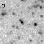
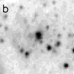
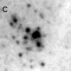
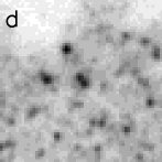
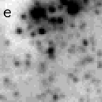
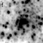
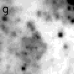
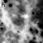
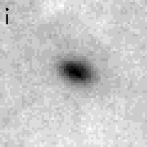
Figure 7: A selection of F435W images centered on sources that were rejected from the sample after visual inspection. The size of each image is 60$\times$60 pixels or 3″$\times$3″. Rejection was based on the following criteria: a. neighbour too close by, b. likely blended, c & d. clearly blended, e. too irregular, f. crowded, g. interfering background, h. radius fit on the background and i. likely a background galaxy.

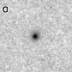
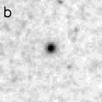
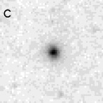
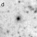
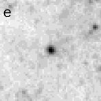
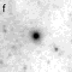
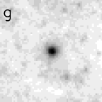
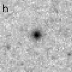
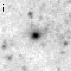
Figure 8: A selection of isolated stellar cluster candidates in F435W that passed the visual inspection. The size of each image is 60$\times$60 pixels or 3″$\times$3″.

In Table 2 we summarize the results of our sample selection for the radius sample. Our final sample of stellar cluster candidates with accurate radii consists of 1284 sources, of which 57% are located in the high background region and 25% in the low background region. From here on we will refer to this sample of stellar cluster candidates simply as “clusters”. The larger sample of resolved sources, which does not satisfy the radius difference criterion (criterion 4) and which magnitude cutoffs follow the 90% completeness limits (criterium 3), consists of 7698, 6846 and 5024 sources in F435W, F555W and F814W, respectively. This sample will be studied in a different paper (Haas et al. 2007, in prep.).

Table 2: The selection of the sample of stellar cluster candidates with accurate radii. The numbers indicate the amount of sources that satisfy the mentioned criterion and all the criteria mentioned above it, split in the low, intermediate and high background region.

Criterion		Nr. remaining
	low	inter	high
All sources	35 980	15 809	23 647
$\mbox{$R_{\mathrm{eff}}$}>0.5$ pc	11064	4799	7238
$\chi^{2}/\chi_{0}^{2}<1$	10715	4661	7028
$\emph{F435W}<22.5$ mag
$\emph{F555W}<22.3$ mag	472	346	1301
$\emph{F814W}<22.7$ mag
$|R_{\emph{F435W}}-R_{\emph{F555W}}|<2$ pc	457	327	1068
No neighbour within 5 pixels	418	302	939
After visual inspection	317	239	728
Total sample: 1284

5.2 Old Globular Clusters and Faint Fuzzies

To see if there are any possible old ($\gtrsim 10$ Gyr) GC candidates in our cluster sample, we applied the colour criteria $\mbox{$B\!-\!V$}>0.5$ and $\mbox{$V\!-\!I$}>0.8$ to our cluster sample, typical for old MW GCs. There are only 70 clusters satisfying these criteria, showing that the majority of our cluster sample consists of young clusters, but a small fraction of $\sim$5% is probably part of an old GC population or highly reddened. A more detailed identification of GC candidates in M51 will be carried out in future studies.

We note that our dataset covers the same field used by Hwang & Lee (2006, from here on referred to as “HL06”), who detect 49 “faint fuzzy” star clusters around the companion of M51, NGC 5195. Faint fuzzy clusters were introduced by Larsen & Brodie (2000), because they formed a sub-group in a radius-colour diagram of star clusters in NGC 1023. In Fig. 9 we show $R_{\mathrm{eff}}$ versus $V\!-\!I$ for the clusters in our sample. Six clusters in our sample satisfy the criteria of a faint fuzzy, namely $0.6<\mbox{$B\!-\!V$}<1.1$, $1.0<\mbox{$V\!-\!I$}<1.5$ and $\mbox{$R_{\mathrm{eff}}$}>7$ pc. These faint fuzzy candidates are indicated in Fig. 9. The figure shows that the faint fuzzy candidates indeed form a separate group in a radius-colour diagram and are not simply the largest clusters in the tail of a continuous radius distribution.

Figure 9: $R_{\mathrm{eff}}$ versus $V\!-\!I$ colour for the total sample of 1284 clusters. The upper-right corner of the dashed lines indicate the region of the sub-group of faint fuzzy candidates (filled circles). These cuts are the same as used by Hwang & Lee (2006) to select faint fuzzy clusters in NGC 5195.

The six faint fuzzy candidates seem randomly located in (or projected onto) the disc of M51. None of the 49 faint fuzzy candidates of HL06 are therefore recovered in our cluster sample. This is because all these 49 candidates are fainter than the magnitude limits we apply. This is expected, since we apply rather conservative magnitude limits in order to achieve accurate radius measurements, also for large clusters in high background regions (§ 5.1). If we would drop our conservative magnitude limits from the selection criteria, we would have 37 of the 49 faint fuzzy candidates from HL06 in our sample. The 12 remaining candidates are removed from our sample based on “inaccurate radii” criteria (large radius difference between F435W and F555W or a $\chi^{2}$ larger than $\chi_{0}^{2}$). The six faint fuzzy candidates in our sample are not in the sample of HL06, because these authors focused on the region around NGC 5195 and were therefore not covering the disc of M51.

5.3 The largest cluster: 212995

One cluster candidate in our radius sample, with our ID number “212995”, clearly stands out from the other cluster candidates in radius. The cluster candidate, positioned at RA=13^h29^m51$\aas@@fstack{s}$94, Dec=+47°11′19$\aas@@fstack{\prime\prime}$63 and shown in Fig. 10, has an (ellipticity corrected) $\mbox{$R_{\mathrm{eff}}$}=21.6$ pc in F435W. The projected galactocentric distance of this cluster candidate is 1.02 kpc. Its brightness in F435W, F555W and F814W is 22.27, 21.52 and 20.48 mag, respectively, with corresponding $B\!-\!V$ and $V\!-\!I$ of 0.75 and 1.05, respectively. These colours make this source both an old GC and faint fuzzy candidate. Assuming the source is a cluster, we can make an estimate of its age and mass by using GALEV SSP models. However, since we only have photometry in three filters, this estimate suffers from an age-extinction-metallicity degeneracy, introducing rather large uncertainties. Assuming a low extinction ($E(B-V)<0.1$) and a metallicity in the range of 0.2–1.0 $\mathrm{Z_{\sun}}$, the best estimate for the age is $2.7^{+2.8}_{-1.8}$ Gyr. The corresponding best estimate for the mass is $2.5^{+3.3}_{-1.1}$$\times 10^{5}\leavevmode\nobreak\ \mathrm{M_{\sun}}$, which is a lower limit due to the underestimation of the aperture correction for the photometry for such a large source. Assuming the metallicity is $0.02\leavevmode\nobreak\ \mathrm{Z_{\sun}}$, the best estimates for the age and mass are $13.2^{+2.8}_{-9.7}$ Gyr and $8.0^{+3.5}_{-4.6}$$\times 10^{5}\leavevmode\nobreak\ \mathrm{M_{\sun}}$, respectively. However, the possibility of the source being a highly reddened young cluster is not fully excluded. There is also a possibility that this cluster candidate is actually a background galaxy, but this possibility is considered to be unlikely, since the cluster is located (in projection) very close to the centre of M51, where the extinction of the background source and the surface brightness of the foreground (M51) is high.

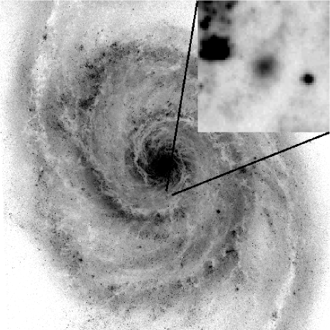
Figure 10: Cluster “212995”, the largest cluster in our sample with a $\mbox{$R_{\mathrm{eff}}$}=21.6$ pc (centre of the inset), and its location in M51 (north is up, east is to the right). The projected galactocentric distance is 1.02 kpc. The scale of the inset image is $\sim 60\times 60$ pixels or $\sim 122\times 122$ pc. The scale of the big image is $\sim 16\times 16$ kpc.

6 A comparison between ACS and WFPC2

As a test of the robustness of our methods, we compared the photometry and the radii of our clusters to the data of B05. B05 derived ages, masses, extinctions and effective radius estimates of stellar clusters covering the central $\sim 7.3\times 8.1$ kpc of M51 using HST NICMOS and WFPC2 data. We calculated the transformation between a mosaic of the F555W WFPC2 images and the ACS mosaic image with the GEOMAP task in IRAF, by identifying 10 sources by eye that were clearly visible in both data sets. We then transformed the coordinates of all the clusters in their sample to our ACS mosaic frame using the GEOXYTRAN task in IRAF, and we matched sources which were within 1 pixels from a cluster in our sample, which had photometry in F435W ($\approx B$), F555W ($\approx V$) and F814W ($\approx I$) in both data sets and which had a measured radius on the WFPC2 data $0<\mbox{$R_{\mathrm{eff}}$}<12$ pc. This resulted in 271 matched clusters, of which a few will be mismatched due to the uncertainties in the transformation and most importantly, geometric distortion of the WFPC2 images.

For these 271 clusters we compared the $B\!-\!V$ and $V\!-\!I$ colours of B05 with our results, after we removed our filter dependent infinity corrections and Galactic foreground extinction corrections, since these were constant for the photometry of B05. In Fig. 11 we plot the difference between the ACS and WFPC2 colours versus the ACS colour. For the mean differences we find:

$$\Delta(B\!-\!V)=(B\!-\!V)_{ACS}-(B\!-\!V)_{WFPC2} = -0.005\pm 0.005$$

$$\Delta(V\!-\!I)=(V\!-\!I)_{ACS}-(V\!-\!I)_{WFPC2} = 0.064\pm 0.006,$$

where the errors are the standard errors of the means, not to be confused with the standard deviations, which are $0.076$ and $0.098$, respectively. This shows that our colours are in good agreement with B05 and that we can adopt the masses derived by B05 for these 271 clusters to study the mass-radius relation with the higher resolution of the ACS data in § 8.2.

Figure 11: The differences between the colours of clusters matched between our ACS dataset and the WFPC2 dataset of Bastian et al. (2005), versus the colour in the ACS dataset.The dashed lines show a difference of 0 as a reference for the eye.

We also compared the effective radii of the 271 matched clusters on the F555W image. In Fig. 12 we show the difference between the ACS and WFPC2 radius versus the ACS radius. No clear trend is visible, except that the average ACS radius of the clusters is slightly smaller than the WFPC2 radius. The mean difference between the ACS and WFPC2 radius is

$$\mbox{$R_{\mathrm{eff}}$}_{,ACS}-\mbox{$R_{\mathrm{eff}}$}_{,WFPC2}=-0.34\pm 0.06\leavevmode\nobreak\ \mathrm{pc},$$

where the error is the standard error of the mean. The standard deviation around the mean is $0.94$ pc. We note that some of the differences between ACS and WFPC2 radii are expected to be caused by contaminants in the matching procedure, as well as resolution effects (blends in the WFPC2 data) and a different treatment of ellipticity for both data sets. For the WFPC2 data circular cluster profiles were assumed, while for the ACS data we used elliptical profiles with a transformation to a single $R_{\mathrm{eff}}$. Overall, the mean difference between the ACS and WFPC2 radii is within the expected accuracy of the radius measurements ($\sim 0.5$ pc), and Fig. 12 suggests that there are no strong radius dependent biases in our methods.

Figure 12: The differences between the effective radii of the clusters matched between our ACS dataset and the WFPC2 dataset of Bastian et al. (2005), versus the effective radius in the ACS dataset.

7 The radius distribution

Now that we have selected a sample of clusters with accurate radii, we will study the distribution of their radii and possible dependencies between radius, background region and colour in this section. Possible correlations between radius and luminosity, mass and galactocentric distance will be the subject of the next section.

We show the effective radius distribution of our sample of 1284 clusters with linear bins in Fig. 14 and with logarithmic bins in Fig. 14. In both figures we plot the radius distributions for cluster in the low and high background region separately. We see that the radius distribution peaks around 1–2 pc and then drops to a maximum radius of $\sim$10 pc. In the remainder of this section we will first focus on the slope of the radius distribution at $\mbox{$R_{\mathrm{eff}}$}>3$ pc and then focus on the location of the peak.

Figure 13: The effective radius distribution of the total sample of 1284 clusters, measured on the F435W image, using linear radius bins (solid line). Also shown are the radius distribution of only the sources in the low background region (dotted line) and the sources in the high background region (dashed line). For better readability, only the (Poissonian) error bars of the total sample are shown.

Figure 14: The effective radius distribution of the total sample of 1284 clusters, measured on the F435W image, using logarithmic radius bins (solid line). Also shown are the radius distribution of only the sources in the low background region (dotted line) and the sources in the high background region (dashed line). For better readability, only the (Poissonian) error bars of the total sample are shown. For comparison we also show a power law with a slope of $-2.3$, typical for a fractal radius distribution of star-forming gas clouds, and a slope of $-1.2$ as determined by B05 for the radius distribution of 407 star clusters in M51 with WFPC2 data.

7.1 The slope of the radius distribution

It has been observed that the mass distributions of both star-forming clouds (Sanders et al. 1985; Solomon et al. 1987; Harris & Pudritz 1994; Brand & Wouterloot 1995; Elmegreen & Falgarone 1996; Fukui et al. 2001) and star clusters (Zhang & Fall 1999; Ashman & Zepf 2001; Bik et al. 2003; de Grijs et al. 2003; Hunter et al. 2003) can be approximated by power laws of the form $N(M)\mathrm{d}M\propto M^{-\alpha}\mathrm{d}M$, with the index $\alpha$ in the range of 1.5–2.0. Star-forming clouds also show a power-law radius distribution of the form $N(R)\mathrm{d}\log R\propto R^{-2.3}\mathrm{d}\log R$ (Harris & Pudritz 1994; Elmegreen & Falgarone 1996). For the clouds, the power-law mass and radius distributions are consistent with the clouds having a fractal structure with a fractal dimension of 2.3 (Mandelbrot 1983; Elmegreen & Elmegreen 2001). Since the mass distribution of clusters is similar to the mass distribution of clouds, one might naively expect the radius distributions also to be similar. We plotted the radius distribution of star clusters in M51 in Fig. 14, using logarithmic bins. In this figure a power law would be a straight line. We plotted two lines with a slope of $-2.3$ and $-1.2$. The first slope is consistent with the power-law distribution of the form $N(R)\mathrm{d}\log R\propto R^{-2.3}\mathrm{d}\log R$ or $N(R)\mathrm{d}R\propto R^{-3.3}\mathrm{d}R$, observed for star-forming gas clouds on every length scale (down to the smallest scales of $\sim 0.1$ pc). We see in Fig. 14 that the radius distribution of the clusters in M51 between $\sim$3 and $\sim$10 pc can not be approximated by the same power law as the one for the star-forming gas clouds.

The slope of $-1.2$, indicated in Fig. 14, is consistent with the power-law distribution of $N(R)\mathrm{d}R\propto R^{-2.2}\mathrm{d}R$, found by B05 for 407 clusters between 2–15 pc in M51 using WFPC2 data. Although the slope of our observed radius distribution in the range $\sim 3$–6 pc is similar to the slope observed by B05, our observed radius distribution is considerably steeper at larger radii. However, we note that we used a larger sample of clusters, measured at twice the resolution and which was checked by visual inspection for contaminants and blends. The cluster sample of B05 is therefore expected to have a larger fraction of contaminants and blends than the current sample. We note however, that the current sample is still biased against clusters in crowded regions, but for the remainder of this study we assume that the current sample is representative of the entire star cluster population of M51.

Fig. 14 shows that the radius distribution of star clusters in M51 is not consistent with a fractal structure. This suggests that after the formation of the clusters from a fractal gas, their radii have changed in a non-uniform way. Unfortunately, at the small radius end of the distribution a possible bias against small clusters can not be completely ruled out, since in a fractal gas the smallest clusters are expected to form in groups closest together. These small clusters could have been rejected from our sample by the close neighbour criterion (§ 5). Without this criterion, however, our sample would also be biased against small clusters due to blends. This bias is not expected at the large radius end of the distribution, where the radius distribution of star clusters in M51 is clearly not consistent with a fractal distribution.

The picture in which the radii of the clusters change shortly after their formation is consistent with various suggested explanations for the lack of the mass-radius relation of clusters (see § 8.2). One possible explanation is that interactions between young star clusters and gas clouds lead to dynamical heating and therefore expansion of the clusters (e.g. Gieles et al. 2006b). This expansion will be strongest for the largest and least concentrated clusters because of their lower density and it will therefore make an initial power-law distribution more shallow. Although cluster-cloud interactions are probably part of the explanation for the lacking mass-radius relation, on its own this scenario fails to explain the expansion of the smallest clusters, which is necessary to weaken the mass-radius relation.

Another suggested explanation for the weak or missing mass-radius relation of clusters is a star formation efficiency (SFE) which scales with the mass of the clouds (Ashman & Zepf 2001) combined with the early residual gas loss from clusters (Hills 1980; Geyer & Burkert 2001; Goodwin & Bastian 2006). In this scenario the forming clusters initially follow the same mass-radius relation as the clouds. However, the removal of binding energy will lead to the expansion of preferably small clusters, since they form from low-mass clouds which lose relatively more residual gas. On its own, however, this explanation will lead to a steeper radius distribution of clusters compared to clouds, i.e. with a slope $<-2.3$, contrary to what we observe (Fig. 14).

Although Fig. 14 suggests that the radii of the clusters have changed shortly after their formation, our radius distribution is consistent with neither scenario. Perhaps a scenario including a combination of stochastic cluster-cloud interactions, expansion due to residual gas expulsion and a mass-dependent SFE can change the radius distribution in a way that is more consistent with the observed radius distribution. However, a fundamental problem of the missing mass-radius relation of clusters is that there are also high-mass clusters with small radii. The existence of these clusters can not be explained by the scenarios mentioned so far, which all rely on the expansion of clusters. Therefore, we need better scenarios and more insight in cluster formation theory to account for the differences in the radius distributions between clouds and clusters.

7.2 The peak of the radius distribution

In Fig. 14 we see that there is a peak in the radius distribution around $\sim$1.5 pc. If we assume that the star clusters in M51 formed from a fractal gas, this is consistent with the suggestion of the expansion of preferably the smallest clusters, i.e. cluster with $\mbox{$R_{\mathrm{eff}}$}<1.5$ pc which expanded to radii $>$1.5 pc.

Fig. 14 and 14 also show that the radius distribution of clusters in the low background region (the dotted lines) shows a more pronounced turnover, i.e. there are relatively fewer small clusters in the low background region compared to the high background region. This suggests that generally the smallest clusters are mainly found in the high background regions (e.g. inside the spiral arms). The medians also show this trend: while the median $R_{\mathrm{eff}}$ of our complete cluster sample is 2.1 pc, it is 1.9 pc for the high background and 2.7 pc for the low background region.

We stress that it is not very likely that this trend is biased due to selection effects, since we applied magnitude limits that are brighter than the 90% completeness limits in the high background region (§ 4), and visual inspection removed most background galaxies in the low background region and possible blends in the high background region. Also, the more compact clusters are easier to detect, so it is not likely that there is a selection effect against small clusters in the low background regions.

Fig. 15 shows the $B\!-\!V$ colour distribution of clusters in the low and high background region. The high background region has a higher fraction of blue clusters ($\mbox{$B\!-\!V$}\lesssim 0.05$) than the low background region. This fraction is expected to be stronger when extinction is taken into account, since clusters in the high background region are likely more strongly reddened than clusters in the low background region.

Figure 15: The normalized $B\!-\!V$ colour distribution for clusters in the low (dotted) and high (dashed) background region. The high background region has a higher fraction of blue clusters than the low background region.

Fig. 14 and 15 suggest that there is a relation between $R_{\mathrm{eff}}$ and colour. In Fig. 16 we show the radius distribution for 2 equal-sized samples with $\mbox{$B\!-\!V$}<0.1$ (“blue”) and $\mbox{$B\!-\!V$}>0.1$ (“red”). We indeed see a shift in the radius distribution towards larger radii for our red subsample. The median value follows this shift: for the blue sample the median $R_{\mathrm{eff}}$ is 1.8 pc, while for the red sample it is 2.5 pc. In Fig. 17 we show the median $R_{\mathrm{eff}}$ versus $B\!-\!V$ and $V\!-\!I$ colour. Because all bins contain an equal number of clusters, size-of-sample effects are excluded. Both for low and high background regions and $B\!-\!V$ and $V\!-\!I$ colours we see a similar trend of a median $R_{\mathrm{eff}}$ increasing with colour, although the scatter is high and the trend is strongest for $B\!-\!V$ colours.

Figure 16: The effective radius distribution split in a sample with $\mbox{$B\!-\!V$}<0.1$ (blue, dashed line, 645 clusters) and $\mbox{$B\!-\!V$}>0.1$ (red, dotted line, 639 clusters). The radius distribution of the red sample is shifted towards larger radii.

Figure 17: The median $R_{\mathrm{eff}}$ versus colour for bins containing an equal number of clusters for the complete cluster sample (top) and the low (middle) and high (bottom) background region. The vertical error bars indicate the range in which 68% of the clusters is contained.

Therefore, the observed difference in the radius distribution between low and high background regions can be explained by a higher fraction of red clusters in low background regions, which are generally slightly larger. For young clusters, colours become redder with age. This is consistent with a larger fraction of blue clusters in high background regions, since these regions follow the high density spiral arms, where most clusters are expected to form. If the observed spread in colour is also a spread in the age of the clusters, the slight increase in median $R_{\mathrm{eff}}$ with colour in Fig. 17 suggests a dynamical evolution of the clusters with age. The fact that the increase in radius is strongest for $B\!-\!V$ colours supports this suggestion, because $B\!-\!V$ is more sensitive to age than $V\!-\!I$.

In this hypothesis, newly formed clusters in spiral arms are generally small, reflecting the high pressure and density of their parental gas clouds. In the subsequent early evolution of the clusters an increase in size is expected, likely due to dynamical heating from cluster-cluster and cluster-cloud encounters and due to the removal of binding energy when the clusters lose mass (Goodwin 1997; Boily & Kroupa 2003). Clusters also expand when moving out of the spiral arm, due to tidal forces from the spiral density wave (Gieles et al. 2007). This hypothesis is consistent with the low background regions containing a relatively larger fraction of older, more evolved clusters with therefore slightly larger radii.

If clusters expand, they will do this on a dynamical (crossing) timescale of a few Myrs (Lada & Lada 2003). The typical timescale for a cluster to move from the high to low background region will be about half the time between 2 spiral arm passages, which for a 2-armed spiral galaxy is

$$\tau(R_{\mathrm{G}})=\frac{\pi R_{\mathrm{G}}}{2\left(V_{\mathrm{disc}}-\Omega_{\mathrm{p}}R_{\mathrm{G}}\right)},$$ (4)

in which $V_{\mathrm{disc}}$ is the circular velocity in the disc and $\Omega_{\mathrm{p}}$ is the angular pattern speed. For M51 this gives $\tau(1\leavevmode\nobreak\ \mathrm{kpc})\approx 10$ Myr (using $V=200\leavevmode\nobreak\ \mathrm{km}\,\mathrm{s}^{-1}$ (García-Burillo et al. 1993) and $\Omega_{\mathrm{p}}=37\leavevmode\nobreak\ \mathrm{km}\,\mathrm{s}^{-1}\mathrm{kpc}^{-1}$ (Zimmer et al. 2004)). This is a typical lower-limit for the timescale to move from the high to low background region. For the more average galactocentric distance of 5 kpc, $\tau(5\leavevmode\nobreak\ \mathrm{kpc})\approx 5.2\cdot 10^{8}$ yr. These timescales are longer than the expansion timescale of the clusters, and are therefore consistent with the low background region containing a considerable number of larger clusters than the high background region, if the clusters started expanding shortly after their formation in a spiral arm.

7.3 A radius-age relation?

We have used the 271 matched clusters with an age estimate from B05 to search for a correlation between age and $R_{\mathrm{eff}}$. These clusters show a weak relation between radius and age of the form $\mbox{$R_{\mathrm{eff}}$}\propto\mathrm{age}^{0.08\pm 0.03}$, with a large scatter. This is consistent with the relation Lee et al. (2005) observe for clusters in M51 using WFPC2 data (best fit slope of $0.06\pm 0.02$). Fig. 18 shows the radius distribution for the matched clusters, split in two equal-sized samples with log(age)$<$7.5 and log(age)$>$7.5. The distributions are not very different, although a weak trend is visible since the older sample has slightly more large clusters than the younger sample. However, these differences are within the statistical errors and also a K-S test did not give a significant result ($p=0.126$). The median $R_{\mathrm{eff}}$ follows a similar trend: the median $R_{\mathrm{eff}}$ is 1.8 and 2.2 pc for the younger and older population, respectively.

Figure 18: The radius distribution of the 271 matched clusters for which we have age estimates from B05, split in a sample with log(age)$>$7.5 and log(age)$<$7.5.

7.4 A comparison with other results

We compared the mean and median $R_{\mathrm{eff}}$ of our cluster sample to other work, but we note that these comparisons can easily be biased by differences in the lower limits of the radius and other selection criteria. The mean and median $R_{\mathrm{eff}}$ of our total sample are 2.5 and 2.1 pc, respectively. The mean and median $R_{\mathrm{eff}}$ of the 70 GC candidates in our sample are $3.7\pm 0.4$ and 2.4 pc, respectively, where $0.4$ is the standard error of the mean (the standard deviation is 3.4 pc). If we restrict ourselves to clusters in the low background regions, the mean and median $R_{\mathrm{eff}}$ are 2.9 and 2.7 pc, respectively. This last value is the same as the mean $R_{\mathrm{eff}}$ Jordán et al. (2005) found for thousands of GCs observed in 100 early-type galaxies of the ACS Virgo Cluster Survey. Larsen (2004) studied the effective radii of stellar clusters in 18 nearby spiral galaxies using HST WFPC2 images, and he found a mean $R_{\mathrm{eff}}$ of $3.94\pm 0.12$ pc. Lee et al. (2005) studied the radii of clusters in M51 using HST WFPC2 observations covering parts of the mosaic image used in our study, and they found a mean and median $R_{\mathrm{eff}}$ of 3.7 and 3.1 pc, respectively. The ACS camera has about twice the resolution of the WFPC2 camera and can therefore detect small clusters more efficiently. This could explain why our mean and median $R_{\mathrm{eff}}$ are smaller than the values from Lee et al. (2005). The median $R_{\mathrm{eff}}$ for Galactic GCs is $\sim$3.3 pc (Harris 1996), very similar to the value Barmby et al. (2006) found for their sample of blue clusters in M101, namely 3.2 pc. We see that the mean and median values of $R_{\mathrm{eff}}$ of our cluster sample are somewhat smaller than what is generally found, although the differences become smaller when we restrict ourselves to the clusters in the low background regions or the GC candidates.

8 Correlations between mass, radius and distance

In this section we will combine the effective radii of the clusters with other parameters, such as their galactocentric distance, luminosity and for some clusters their mass. Correlations between these parameters for clusters in M51 have already been studied by B05, using WFPC2 data of the inner 5 kpc of the disc of M51. We again search for correlations, but now using the ACS data out to a galactocentric distance of $\sim$10 kpc.

8.1 Galactocentric distance

For Galactic GCs there is a relation between the distance to the Galactic centre, $R_{\mathrm{G}}$, and the half-light diameter $D_{0.5}$, of the form $D_{0.5}\propto R_{\mathrm{G}}^{1/2}$ (Van den Bergh et al. 1991). This same trend is observed for the core radii of old clusters in the LMC (Hodge 1962; Mateo 1987) and for the sizes of old GCs in NGC 5128 (Hesser et al. 1984). However, these cluster populations are all old and mainly residing in the outer regions or halo of their host galaxies, while we are studying a population of mostly young clusters in a disc.

For the GCs, different explanations for the observed relation between radius and galactocentric distance have been suggested. One possibility could be that the sizes of GCs reflect the densities of the gas clouds from which they formed, i.e. compact GCs preferentially formed from dense gas clouds near the centres of galaxies, while larger GCs preferentially formed in the less dense halo regions (Van den Bergh et al. 1991). Harris & Pudritz (1994) use the Ebert-Bonnor relations (Ebert 1955; Bonnor 1956) to show that

$$R_{\mathrm{GMC}}\propto M_{\mathrm{GMC}}^{1/2}P_{s}^{-1/4},$$ (5)

in which $R_{\mathrm{GMC}}$, $M_{\mathrm{GMC}}$ and $P_{s}$ are the radius, mass and surface pressure of the gas clouds, respectively. The Van den Bergh relation then arises naturally if the clusters form from gas clouds of which the surface pressure scales with the ISM pressure ($P_{s}\approx 5$–$10P_{ISM}$), which in turn scales as

$$P_{ISM}\propto R_{\mathrm{G}}^{-2}$$ (6)

for the halo region (Harris & Pudritz 1994). From Eq. 5 and 6 and the observation that the mean GC mass does not change with galactocentric distance (Harris & Pudritz 1994), the Van den Bergh relation follows. However, models like these assume that the relations with surface pressure are also valid in the cloud cores, where the clusters actually form, but this assumption is not necessarily valid.

Another possible explanation for the observed relation between radius and galactocentric distance for GCs is more evolutionary in nature. It assumes that the GCs have reached tidal equilibrium with their host galaxy. The tidal radius of a cluster in an external logarithmic potential field scales as:

$$r_{\mathrm{t}}\propto M_{\mathrm{cl}}^{1/3}R_{\mathrm{G}}^{2/3},$$ (7)

where $M_{\mathrm{cl}}$ is the cluster mass (Binney & Tremaine 1987, chap. 7.3). Thus, when a cluster is relaxed, in tidal equilibrium with its host galaxy and filling its Roche lobe, its tidal radius is expected to scale as $r_{\mathrm{t}}\propto R_{\mathrm{G}}^{2/3}$. We would also expect the effective radius to scale as $\mbox{$R_{\mathrm{eff}}$}\propto R_{\mathrm{G}}^{2/3}$, only if the density profile of the cluster would be constant and if the cluster is in tidal equilibrium with the galaxy. For young clusters in the disc, however, the validity of these assumptions remains to be seen.

In Fig. 19 we show the median $R_{\mathrm{eff}}$ versus the galactocentric distance for the clusters in M51. There seems to be a slight increase in $R_{\mathrm{eff}}$ with distance, but the scatter is large (reflected in the large error bars). We have tried to fit a function of the form

$$\frac{\mbox{$R_{\mathrm{eff}}$}}{\mathrm{1\leavevmode\nobreak\ pc}}=c\cdot\left(\frac{R_{\mathrm{G}}}{\mathrm{1\leavevmode\nobreak\ kpc}}\right)^{\alpha}$$ (8)

to the unbinned data, in which $c$ is a constant, and for the best fit we find $\alpha=0.12\pm 0.02$. This relation is significantly weaker than the predicted $\alpha=0.67$ (for GCs in tidal equilibrium) or the observed relation for Galactic GCs ($\alpha=0.5$).

Figure 19: The median $R_{\mathrm{eff}}$ versus galactocentric distance, for bins containing an equal number of clusters. The vertical error bars indicate the range in which 68% of the clusters is contained.

The radius distribution changes for different galactocentric distance bins, as shown in Fig. 20. The radius distribution close to the centre of M51 (distance $<$ 3 kpc) is shifted towards smaller radii compared to the radius distributions at larger distances. A K-S test confirmed that it is unlikely ($p<0.001$) that the radius distribution for distance $<$ 3 kpc and $>$ 5.5 kpc are drawn from the same parent distribution.

Figure 20: The effective radius distributions for three different galactocentric distance regions in M51. The solid line shows clusters close to the centre of M51 (distance $<$ 3 kpc), the dotted line shows clusters at intermediate distances (3$<$ distance $<$5.5 kpc) and the dashed line shows clusters at large galactocentric distances ($>$ 5.5 kpc). The changes in the distributions are consistent with a slight increase in $R_{\mathrm{eff}}$ with distance.

Since we observe a relation between $R_{\mathrm{eff}}$ and color (Fig.17), any increase in radius with galactocentric distance could be the result of an increase in colour with galactocentric distance. In Fig. 21 we show $B\!-\!V$ versus galactocentric distance for the 1284 clusters that were also shown in Fig. 19. No obvious trend is visible, which is expected since at all galactocentric radii we encounter clusters in both arm and interarm regions. The arm regions are mostly high background regions and will therefore contain mostly blue clusters, while the interarm regions are mostly low background regions and will therefore contain mostly red clusters (Fig 15). The observed $\mbox{$R_{\mathrm{eff}}$}\propto R_{\mathrm{G}}^{0.12\pm 0.02}$ is therefore not likely a result of the relation between radius and colour.

Figure 21: The median $B\!-\!V$ colour versus galactocentric distance of the 1284 clusters in our sample for bins containing an equal number of clusters. The vertical error bars indicate the range in which 68% of the clusters is contained. No obvious trend is visible in the data.

B05 did not find a relation between $R_{\mathrm{eff}}$ and $R_{\mathrm{G}}$ for $R_{\mathrm{G}}<5$ kpc. For $R_{\mathrm{G}}\lesssim 13$ kpc we find a weak relation, but this relation is considerably weaker than the observed relations for old GCs. Therefore, the clusters we observe in the disc of M51 are either forming under different conditions than the GCs, or the observed relation for GCs emerged during their longer dynamical evolution. We consider the first explanation to be the most likely one, since GCs probably formed outside a spiral disc, in regions where the surface pressure of their parental clouds decreased with distance (Eq. 6). For clusters in spiral arms it is not expected that the surface pressure scales in a similar way with distance. Likely, the higher pressure inside spiral arms decreases less strongly with galactocentric distance. Rix & Rieke (1993) find that the arm/interarm density contrast for M51 increases with galactocentric distance, consistent with this picture. In this case a strong radius-distance correlation for the clusters is not expected.

8.2 Mass-radius relation

One of the most peculiar properties of star clusters is the lack of a clear relation between their mass and radius. Star clusters are believed to form from Giant Molecular Clouds (GMCs), for which a clear relation between mass and radius is observed. Larson (1981) finds that the internal velocity dispersion of GMCs, $\sigma$, scales with their size, $R_{\mathrm{GMC}}$, as $\sigma\propto R_{\mathrm{GMC}}^{0.38}$. Assuming the GMCs are in virial equilibrium, this leads to a mass-radius relation of the form $R_{\mathrm{GMC}}\propto M_{\mathrm{GMC}}^{0.57}$. Also assuming virial equilibrium, Solomon et al. (1987) find $R_{\mathrm{GMC}}\leavevmode\nobreak\ =\leavevmode\nobreak\ 1/540\cdot M_{\mathrm{GMC}}^{0.5}$. These observations are consistent with GMCs having a constant surface density ($\Sigma\equiv M_{\mathrm{GMC}}/\pi R_{\mathrm{GMC}}^{2}$).

From the Ebert-Bonnor relations for pressure bounded, self-gravitating, isothermal spheres (Ebert 1955; Bonnor 1956), both Eq. 5 as well as:

$$\Sigma\propto P_{s}^{1/2}$$ (9)

can be derived, in which $P_{s}$ is the surface pressure (Harris & Pudritz 1994; Ashman & Zepf 2001). So the observed mass-radius relation and constant surface density for clouds are expected if the surface pressure is constant (Elmegreen 1989).

When clusters emerge from GMCs, the mass-radius relation appears to be erased, indicating that high-mass clusters have higher stellar densities than low-mass clusters. A constant stellar density would predict $\mbox{$R_{\mathrm{eff}}$}\propto M_{\mathrm{cl}}^{1/3}$, which is not observed. Zepf et al. (1999) find $\mbox{$R_{\mathrm{eff}}$}\propto L^{0.07}$ for young clusters in NGC 3256, where $L$ is the luminosity of the cluster which scales directly with the mass (since their cluster sample suggests that colour is independent of luminosity and therefore they assume that the mass-to-light ratio is mostly independent on luminosity). For clusters in a sample of (non-interacting) spiral galaxies, Larsen (2004) finds $\mbox{$R_{\mathrm{eff}}$}\propto M_{\mathrm{cl}}^{0.10\pm 0.03}$. The effective radius of the old Galactic GCs also does not seem to correlate with their luminosity and thus their mass (Van den Bergh et al. 1991). Mackey & Gilmore (2003) report that for a sample of 53 rich LMC clusters, there seems to be no strong correlation between their mass and core radius, either.

In Fig. 22 we show $R_{\mathrm{eff}}$ versus magnitude in F435W for the M51 clusters, split in the low and high background region. For these clusters we do not have mass estimates. However, it is expected that the age range for the largest fraction of this cluster sample is not very large, because most clusters are blue and located in the spiral arms. Many clusters are therefore expected to have similar mass-to-light ratios and therefore any mass-radius relation should also be visible as a relation between magnitude and radius. Fig. 22 shows that clusters in the high background regions show a slight trend of radius decreasing with luminosity. Clusters in the low background regions show a less obvious trend, although the median $R_{\mathrm{eff}}$ of the brightest bin is considerably larger, especially compared to the brightest bin in the high background region. A fit on the unbinned data points of the form $\mbox{$R_{\mathrm{eff}}$}\propto L^{x}$, with $L$ the luminosity in the F435W passband, resulted in $x=0.15\pm 0.02$ and $x=-0.11\pm 0.01$ for the low and high background region, respectively. We verified that applying the size-dependent aperture correction of Eq. 2.5, instead of the constant aperture correction for a 3 pc source (§ 2.5), would not change this result considerably ($x=0.13\pm 0.02$ and $x=-0.10\pm 0.01$ for the low and high background, respectively).

Figure 22: The median $R_{\mathrm{eff}}$ versus F435W magnitude for our sample of 317 clusters in the low background region (top) and for our sample of 728 clusters in the high background region. The bins contain an equal number of clusters and the vertical error bars indicate the range in which 68% of the clusters is contained.

It is not likely that this observed differences in power-law indices is a bias due to our detection limits, since we use magnitude limits (§ 5.1) brighter than the 90% completeness limits for $\sim$8 pc sources in the high background regions. Due to the lack of age estimates of these clusters, there is a degeneracy between age and mass. Therefore it is not certain if any evolution in $R_{\mathrm{eff}}$ with luminosity is mainly caused by age effects, mass effects, or a combination of both. More measurements of the ages and masses of clusters which also have accurate radii estimates are necessary to break this age/mass degeneracy (e.g. through additional $U$-band imaging).

Using the 271 clusters that were matched with the cluster sample of B05 and for which we therefore have mass estimates, we show $R_{\mathrm{eff}}$ versus mass in Fig. 23. No apparent relation is visible. This sample is too small to make a distinction between clusters in low and high background regions, since it mostly covers the inner high background regions of M51.

Figure 23: $R_{\mathrm{eff}}$ versus mass for the 271 clusters that were matched with the cluster sample of B05.

We conclude that we do not find evidence for any direct relation between mass and radius of the clusters, although we find weak relations between luminosity and radius, changing with background region. The suggested explanations for a lacking mass-radius relation were already mentioned in § 7.1, but we stress again that none of these scenarios are currently capable of explaining the observed differences in the radius distributions between clouds and clusters.

9 Summary and conclusions

We have used the HST ACS mosaic image of M51 to detect 7698, 6846 and 5024 stellar clusters across the spiral disc in F435W, F555W and F814W  respectively, based on effective radius ($R_{\mathrm{eff}}$) measurements. We presented the dataset and described the methods used to select our cluster sample, including tests with artificial clusters to show the accuracy, limits and robustness of our methods. We divided the data in 3 regions with respectively a low, intermediate and high background, where the high background traces the spiral arms. We selected a sample of 1284 clusters with the most accurate radius estimates to study the radius distribution and relations between radius, mass, luminosity, galactocentric distance and background region. From these studies we conclude the following:

1. The effective radii of the clusters are distributed between our fixed lower limit of 0.5 pc and $\sim$10 pc (Fig. 14). The mean and median $R_{\mathrm{eff}}$ of our accurate radii sample are 2.5 and 2.1 pc, respectively. This is smaller than what is generally found for young clusters in spiral galaxies.

2. The radius distribution of clusters in M51 can not be fitted with a power law similar as the one for star-forming gas clouds. This suggests that shortly after the formation of the clusters from a fractal gas, their radii have have changed in a non-uniform way.

3. 70 clusters in our sample satisfy the colour criteria for being old GCs. These clusters are slightly larger than the rest of the cluster sample (median $\mbox{$R_{\mathrm{eff}}$}=2.4$ pc). We find 6 clusters in our sample satisfying the criteria for being “faint fuzzy” star clusters projected onto the disc of M51 (Fig. 9).

4. The largest cluster in our sample has $\mbox{$R_{\mathrm{eff}}$}=21.6$ pc and a projected galactocentric distance of 1.02 kpc (Fig. 10). Assuming low extinction and metallicity ($E(B-V)<0.1$, $Z=$ 0.2–1.0 $\mathrm{Z_{\sun}}$), we estimate its age to be $2.7^{+2.8}_{-1.8}$ Gyr and its mass to be $2.5^{+3.3}_{-1.1}$$\times 10^{5}\leavevmode\nobreak\ \mathrm{M_{\sun}}$. Assuming extremely low metallicity ($0.02\leavevmode\nobreak\ \mathrm{Z_{\sun}}$) results in $13.2^{+2.8}_{-9.7}$ Gyr and $8.0^{+3.5}_{-4.6}$$\times 10^{5}\leavevmode\nobreak\ \mathrm{M_{\sun}}$, for its age and mass, respectively.

5. Comparing clusters in the low and high background regions, we find that the high background regions, i.e. the spiral arms, have a higher fraction of blue clusters, consistent with the idea that these regions are the preferred formation sites for clusters (Fig. 15).

6. We detect an increase in $R_{\mathrm{eff}}$ with colour, most strongly for $B\!-\!V$. Since we detect most of the redder clusters outside the spiral arms, the median $R_{\mathrm{eff}}$ outside the spiral arms is larger than inside the spiral arms: 2.7 and 1.9 pc, respectively. The radius distribution of clusters in the low background region also shows a more pronounced turnover around 1.5 pc (Fig. 14). We speculate that if the observed spread in colour is also a spread in the ages of the clusters, this observation suggests a dynamical expansion of the clusters with age. In this hypothesis, newly formed clusters in spiral arms are generally small, their radii reflecting the high surrounding pressure of the parental gas clouds. In the subsequent early evolution of the clusters an increase in size is expected, likely due to dynamical heating from cluster-cluster and cluster-cloud encounters and due to the removal of binding energy when the clusters lose mass.

7. We do not observe a strong correlation between $R_{\mathrm{eff}}$ and galactocentric distance for the clusters in the disc of M51 out to $\sim$13 kpc. A weak trend is visible of the form $R_{\mathrm{eff}}\propto R_{\mathrm{G}}^{0.12\pm 0.02}$, but the scatter is large. For old GCs, mainly residing in the outer regions or halo of other galaxies, a steeper relation is observed, possibly caused by the decreasing pressure of their parental gas clouds with galactocentric distance. The weaker relation for the clusters in M51 could be explained by the observation that most of the clusters reside in the spiral arms. Since the spiral arms are expected to have a higher pressure and they extend out to large galactocentric distances, a strong radius-distance correlation is not expected.

8. We do not observe a correlation between cluster mass and radius for the 271 clusters of which we have mass estimates. We find weak relations between cluster luminosity and radius for our sample of 1284 clusters. If fitted with a power law of the form $\mbox{$R_{\mathrm{eff}}$}\propto L^{x}$, we find $x=0.15\pm 0.02$ and $x=-0.11\pm 0.01$ for the low and high background region, respectively (Fig. 22). Explanations of the lack of a strong mass-radius or luminosity-radius relation probably need to be sought in the early dynamical evolution (expansion) of the clusters just after their formation. Current scenarios which focus on the expansion of clusters due to either dynamical heating or the removal of binding energy due to gas expulsion are not consistent with the observed differences in the radius distributions between clouds and clusters.