Transient Charging and Discharging of Spin-polarized Electrons in a Quantum Dot

Abstract

We study spin-polarized transient transport in a quantum dot coupled to two ferromagnetic leads subjected to a rectangular bias voltage pulse. Time-dependent spin-resolved currents, occupations, spin accumulation, and tunneling magnetoresistance (TMR) are calculated using both nonequilibrium Green function and master equation techniques. Both parallel and antiparallel leads’ magnetization alignments are analyzed. Our main findings are: a dynamical spin accumulation that changes sign in time, a short-lived pulse of spin polarized current in the emitter lead (but not in the collector lead), and a dynamical TMR that develops negative values in the transient regime. We also observe that the intra-dot Coulomb interaction can enhance even further the negative values of the TMR.

year number number identifier Date: ]

I Introduction

A variety of new effects and novel devices have been reported during recent years in the context of the emerging field of spintronics.spintronics ; iz04 ; saw01 ; gap98 One of the most challenging milestones in this context is the development of a quantum computer, which would represent a great breakthrough in the processing time of certain mathematical and physical problems.quantumcomp In particular, the electron spin in quantum dots has been proposed as a building block for the implementation of quantum bits (qubits) for quantum computation.dl98 ; hae05 An important recent development is the possibility to coherently control electron states and electron spin in quantum dot systems with a precision up to a single-electron, thus demonstrating the feasibility of qubit implementation in a solid state system.th03 ; jme04 ; mk04 ; rh05 ; fhlk06 ; lpk06 Specifically, these experimental realizations use high-speed voltage pulses to tune the system levels in a coherent cycle for electronic manipulation. Ac-driven quantum dot systems and double barrier structures have also been studied in the context of quantum pumps,js07 ; es06 ; ec05 ; la05 ; ms99 superlattices,rl03 Kondo effect,rl98 ; k200 ; rl01 ; yy01 and spin-polarized transport.zgz04 ; cl04 In addition to this, time-dependent transport has received growing attention in a variety of mesoscopic systems that encompasses, to mention but a few, molecular electronics,cck05 ; khk06 dissipative driven mesoscopic ring,la04 noisy qubits,fkh05 and dynamical Franz-Keldysh effect.apj96

In the context of spintronics a system of particular interest is composed of a quantum dot or a metallic island coupled via tunnel barriers to two ferromagnetic leads (FM-QD-FM). For example, in the nonequilibrium regime the following effects have been discussed: a spin-split Kondo resonance,yu05 ; jm03 a spin-current diode effect,fms06 zero-bias anomaly,iw05 tunnel magnetoresistance (TMR) oscillations,iw06jb98 negative TMR, jv05 spin accumulation,spinacum and so on. In spite of all this activity, to the best of our knowledge, only very little work has been done on spin-polarized transport driven by ac-bias voltages.zgz04 ; cl04 Here we study transient spin-resolved currents, occupations and TMR generated by a voltage pulse applied in one of the ferromagnetic leads. We use two complementary approaches to study the problem: nonequilibrium Green function (NEGF) and the Master Equation (ME). NEGF is used to give an exact solution in the noninteracting case, while the ME, valid in the limit $k_{B}T\gg\Gamma_{0}$ ($\Gamma_{0}$ is the characteristic level width), is used to demonstrate that the results obtained via NEGF are modified only quantitatively, not qualitatively, when Coulomb interaction is accounted in the sequential-tunneling limit. Both parallel (P) and antiparallel (AP) magnetization alignments are considered. In the P case we find a magnitude and sign modulation of the spin accumulation in the dot, while in the AP alignment only the magnitude changes. For the current we observe a spike of spin polarized current in the emitter lead when the system operates in the P configuration. This effect gives rise to a dynamical negative-TMR just after the bias voltage is turned off.

The paper is organized as follow. In Sec. II we describe the formulation based on NEGF, and give explicit formulas for the noninteracting case. In Sec. III(a)-(c) we present numerical results based on Sec. II, and in Sec. III(d) we apply the master equation technique to account Coulomb interaction effects (in the sequential tunneling limit). Finally, in Sec. IV we give some final remarks.

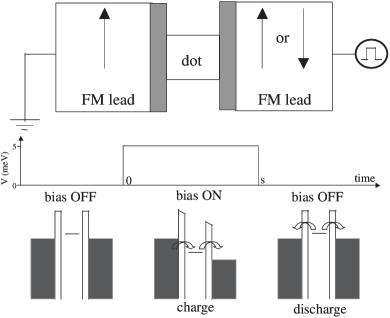
Figure 1: Sketch of the system: a quantum dot coupled to two ferromagnetic leads via tunnel barriers. The left FM lead has its magnetization fixed while the right-hand side can be either in parallel or antiparallel alignment. A pulsed bias voltage of duration $s$ is applied across the system in order to generate transient spin-polarized currents. When the bias voltage is turned on ($0<t<s$) the dot’s level $\epsilon_{d}$ moves into resonance with the emitter states, and the dot becomes populated (a charging process) with a current passing through it. When the bias is turned off ($t>s$) $\epsilon_{d}$ moves above $\mu_{L}$ and $\mu_{R}$ and the dot’s occupation decays into the leads (a discharging process). Due to the ferromagnetism of the leads these transient charging and discharging processes become spin dependent.

II Transport formulation

To describe the system of a quantum dot coupled to two ferromagnetic leads, see Fig. 1, we apply the following Hamiltonian

$$H = \sum_{\mathbf{k}\sigma\eta}\epsilon_{\mathbf{k}\sigma\eta}(t)c_{\mathbf{k}\sigma\eta}^{\dagger}c_{\mathbf{k}\sigma\eta}+\sum_{\sigma}\epsilon_{d}(t)d_{\sigma}^{\dagger}d_{\sigma}$$ (1)

$$+\sum_{\mathbf{k}\sigma\eta}(V_{\mathbf{k}\sigma\eta,\sigma}c_{\mathbf{k}\sigma\eta}^{\dagger}d_{\sigma}+V_{\mathbf{k}\sigma\eta,\sigma}^{*}d_{\sigma}^{\dagger}c_{\mathbf{k}\sigma\eta})$$

$$+Un_{\uparrow}n_{\downarrow},$$

where $\epsilon_{\mathbf{k}\sigma\eta}(t)$ is a time-dependent free-electron energy with wave vector $\mathbf{k}$ and spin $\sigma$ in lead $\eta$ ($\eta=L,R$). This energy can also be written as $\epsilon_{\mathbf{k}\sigma\eta}(t)=\epsilon_{\mathbf{k}\sigma\eta}^{0}+\Delta_{\eta}(t)$, with $\epsilon_{\mathbf{k}\sigma\eta}^{0}$ being the time-independent energy and $\Delta_{\eta}(t)$ gives the time evolution of the external bias. The energy $\epsilon_{d}(t)$ is the time-dependent spin-degenerate dot level, which can also be written as $\epsilon_{d}(t)=\epsilon_{d}^{0}+\Delta_{d}(t)$, where $\epsilon_{d}^{0}$ is the time-independent level and $\Delta_{d}(t)$ follows the bias voltage. It should be noted that in a quantitative theory one should consider a level-shift $\Delta_{d}$, which depends on the level occupation, via some suitable self-consistent procedure. We shall address this issue in our future work, but for the present purpose the simple model suffices.

The operator $c_{\mathbf{k}\sigma\eta}$ ($c_{\mathbf{k}\sigma\eta}^{\dagger}$) is an annihilation (creation) operator for a single-particle momentum state $\mathbf{k}$ and spin $\sigma$ in lead $\eta$ ($\eta=L,R$), and $d_{\sigma}$ ($d_{\sigma}^{\dagger}$) is an annihilation (creation) operator for the single-particle dot’s state $\epsilon_{d}$. The matrix element $V_{\mathbf{k}\sigma\eta,\sigma}$ couples the leads with the dot, and we assume that the tunneling process is spin-independent. Finally, the $U$-term describes the Coulomb repulsion in the dot, with $n_{\sigma}=d_{\sigma}^{\dagger}d_{\sigma}$.

In order to calculate the current we use the definition $I_{\sigma}^{\eta}=-e\langle\dot{N}_{\sigma}^{\eta}\rangle$, where $e$ is the electron charge ($e>0$) and $N_{\sigma}^{\eta}=\sum_{\mathbf{k}}c_{\mathbf{k}\sigma\eta}^{\dagger}c_{\mathbf{k}\sigma\eta}$ is the total number of electrons with spin $\sigma$ in lead $\eta$. From this definition it is straightforward to show thatapj94 ; hh96

$$I_{\sigma}^{\eta}(t)=2e\mathrm{Re}\{\sum_{\mathbf{k}}V_{\mathbf{k}\sigma\eta,\sigma}G_{\sigma,\mathbf{k}\sigma\eta}^{<}(t,t)\},$$ (2)

where

$$G_{\sigma,\mathbf{k}\sigma\eta}^{<}(t,t) = i\int_{-\infty}^{t}dt_{1}V_{\mathbf{k}\sigma\eta,\sigma}^{*}e^{-i\int_{t}^{t_{1}}dt_{2}\epsilon_{\mathbf{k}\sigma\eta}(t_{2})}$$ (3)

$$\times[G_{\sigma\sigma}^{r}(t,t_{1})f_{\eta}(\epsilon_{\mathbf{k}\sigma}^{0})+G_{\sigma\sigma}^{<}(t,t_{1})],$$

with $G_{\sigma\sigma}^{r(<)}(t,t_{1})$ being the retarded (lesser) Green function of the dot and $f_{\eta}(\epsilon_{\mathbf{k}\sigma}^{0})$ is the time-independent Fermi distribution function of lead $\eta$. Substituting Eq. (3) into Eq. (2) and following Ref. [apj94, ] we find

$$I_{\sigma}^{\eta}(t) = -2e\int_{-\infty}^{t}dt_{1}\int\frac{d\epsilon}{2\pi}\mathrm{Im}\{e^{i\epsilon(t-t_{1})}\Gamma_{\sigma}^{\eta}(\epsilon,t_{1},t)$$ (4)

$$\times[G_{\sigma\sigma}^{r}(t,t_{1})f_{\eta}(\epsilon)+G_{\sigma\sigma}^{<}(t,t_{1})]\},$$

with $\Gamma_{\sigma}^{\eta}(\epsilon,t_{1},t)=2\pi\rho_{\sigma\eta}(\epsilon)|V_{\sigma\eta}(\epsilon)|^{2}e^{i\int_{t_{1}}^{t}dt_{2}\Delta_{\eta}(\epsilon,t_{2})}$. These results are exact, and they can in principle be used to study the intricate interplay between time-dependence, coherence and interactions. Their use, however, requires the knowledge of $G^{r}$ and $G^{<}$, which come from the solution of the nonequilibrium Dyson and Keldysh equations, respectively. For our main findings, though, it is sufficient to consider a non-interacting model, for which an exact solution can be obtained. Next, in Sec. 3D, we show that our results change only slightly when Coulomb interaction is included in a master equation based scheme.

In the wideband limit (WBL),wbl ; maciejko06 and for noninteracting electrons Eq. (4) can be written as

$$I_{\sigma}^{\eta}(t)=-e\Gamma_{\sigma}^{\eta}\{\langle n_{\sigma}(t)\rangle+\int\frac{d\epsilon}{\pi}f_{\eta}(\epsilon)\mathrm{Im}[A_{\sigma\eta}(\epsilon,t)]\},$$ (5)

where $\langle n_{\sigma}\rangle$ is the time-dependent dot’s occupation, given by

$$\langle n_{\sigma}(t)\rangle = \mathrm{Im}\{G_{\sigma\sigma}^{<}(t,t)\}$$ (6)

$$= \sum_{\eta}\Gamma_{\sigma}^{\eta}\int\frac{d\epsilon}{2\pi}f_{\eta}(\epsilon)|A_{\sigma\eta}(\epsilon,t)|^{2},$$

and $A_{\sigma\eta}(\epsilon,t)$ is defined as

$$A_{\sigma\eta}(\epsilon,t)=\int_{-\infty}^{t}dt_{1}G_{\sigma\sigma}^{r}(t,t_{1})e^{[i\epsilon(t-t_{1})-i\int_{t}^{t_{1}}d\widetilde{t}\Delta_{\eta}(\widetilde{t})]}.$$ (7)

The retarded Green function in the noninteracting model is given by

$$G_{\sigma\sigma}^{r}(t,t_{1})=-i\theta(t-t_{1})e^{-\frac{\Gamma_{\sigma}}{2}(t-t_{1})}e^{-i\int_{t_{1}}^{t}d\widetilde{t}\epsilon_{d}(\widetilde{t})},$$ (8)

where $\Gamma_{\sigma}=\Gamma_{\sigma}^{L}+\Gamma_{\sigma}^{R}$. For a voltage pulse $V(t)=V_{0}\theta(t)\theta(s-t)$ (see Fig. 1), and assuming that this pulse is applied on the right ferromagnetic lead, with a linear bias drop along the junction, we have $\Delta_{L}(t)=-V_{L}=0$, $\Delta_{R}(t)=-V_{R}(t)=-V(t)$ and $\Delta_{d}=-V_{d}=-V(t)/2$.

With these definitions, we find for $0<t<s$nsw93

$$A_{\sigma\eta}(\epsilon,0<t<s) = \frac{e^{i(\epsilon-\epsilon_{0}+V_{d}-V_{\eta}+i\Gamma_{\sigma}/2)t}}{\epsilon-\epsilon_{0}+i\Gamma_{\sigma}/2}$$ (9)

$$+ \frac{1-e^{i(\epsilon-\epsilon_{0}+V_{d}-V_{\eta}+i\Gamma_{\sigma}/2)t}}{\epsilon-\epsilon_{0}+V_{d}-V_{\eta}+i\Gamma_{\sigma}/2},$$

and for $t>s$ we obtain

$$A_{\sigma\eta}(\epsilon,t>s)=\frac{e^{i(\epsilon-\epsilon_{0}+i\Gamma_{\sigma}/2)t}e^{i(V_{d}-V_{\eta})s}}{\epsilon-\epsilon_{0}+i\Gamma_{\sigma}/2}$$ (10)

$$+ \frac{e^{i(\epsilon-\epsilon_{0}+i\Gamma_{\sigma}/2)(t-s)}-e^{i(V_{d}-V_{\eta})s}e^{i(\epsilon-\epsilon_{0}+i\Gamma_{\sigma}/2)t}}{\epsilon-\epsilon_{0}+V_{d}-V_{\eta}+i\Gamma_{\sigma}/2}$$

$$+ \frac{1-e^{i(\epsilon-\epsilon_{0}+i\Gamma_{\sigma}/2)(t-s)}}{\epsilon-\epsilon_{0}+i\Gamma_{\sigma}/2}.$$

By substituting Eqs. (9) and (10) into Eqs. (5)-(6) yields the final result for the spin-resolved occupations and currents. Numerical results are described in the next section.

III Results

III.1 Parameters

In our numerical calculations we assume that the voltage pulse is applied to the right electrode, so that $\mu_{R}=-V(t)$ while $\mu_{L}$ is kept constant equal zero. The dot’s level is taken originally (zero bias) above the chemical potentials $\mu_{L}$ and $\mu_{R}$, $\epsilon_{0}=0.5$ meV. The temperature is assumed to be $T=2.5K$ $(k_{B}T\approx 215\mu$eV), thus allowing a small thermally excited occupation of the dot in equilibrium. To describe the ferromagnetism of the leads we choose the tunneling rates to be $\Gamma_{\sigma}^{L}=\Gamma_{0}[1+(-1)^{\delta_{\downarrow\sigma}}p]$ and $\Gamma_{\sigma}^{R}=\Gamma_{0}[1\pm(-1)^{\delta_{\downarrow\sigma}}p]$, where $\Gamma_{0}$ is the leads-dot coupling strength and $p$ gives the polarization degree of the leads.wr01 Here we assume a weak coupling with $\Gamma_{0}=1$ $\mu$eV,commentGamma ; typical and a polarization degree $p=0.4$. The $+$ and $-$ signs in $\Gamma_{\sigma}^{R}$ give the parallel and antiparallel configurations, respectively. Due to the ferromagnetism of the leads ($p\neq 0$) we have $\Gamma_{\uparrow}^{L}>\Gamma_{\downarrow}^{L}$ and $\Gamma_{\uparrow}^{R}>\Gamma_{\downarrow}^{R}$ in the parallel case and the opposite $\Gamma_{\uparrow}^{R}<\Gamma_{\downarrow}^{R}$ in the antiparallel alignment. For the bias voltage we adopt $V(t)=V_{0}\theta(t)\theta(s-t)$ where $V_{0}=5$ meV and $s=3$ ns.kbk04 The charging energy $U$ is set equal to zero in Sec. III(b)-(c) and equal to 3 meV in Sec. III(d).

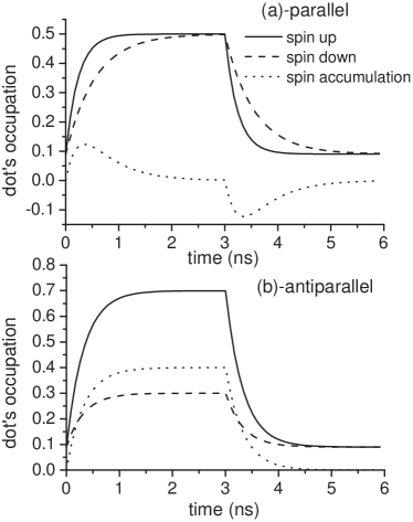
Figure 2: Occupations $n_{\uparrow}$ (solid line) and $n_{\downarrow}$ (dashed line) and the spin accumulation $m=n_{\uparrow}-n_{\downarrow}$ (dotted line) as a function of time for both (a) parallel and (b) antiparallel configurations. When the bias is turned on (off) the dot is charged (discharged) in a spin-dependent manner. This results in a time-dependent spin accumulation, with a sign reversal in the parallel case.

III.2 Spin-polarized occupations

Figure 2 shows the spin-resolved occupations $n_{\uparrow}$ and $n_{\downarrow}$ and the spin accumulation $m=n_{\uparrow}-n_{\downarrow}$ as a function of time for both (a) parallel and (b) antiparallel configurations. Before the bias is turned on the level $\epsilon_{d}$ is above the electrochemical potentials $\mu_{\eta}$ ($\eta=L,R$), and the dot is only slightly occupied due to thermal excitation. When the bias is turned on at $t=0$ the dot’s level is brought into resonance ($\mu_{L}<\epsilon_{d}<\mu_{R}$), thus resulting in an enhancement of $n_{\sigma}$ and $m$. In the parallel case [Fig. 2(a)] the spin up population increases faster than the spin down one, and both attain the same stationary value around 0.5. The steeper enhancement of $n_{\uparrow}$ compared to $n_{\downarrow}$ is related to the inequality $\Gamma_{\uparrow}^{L}>\Gamma_{\downarrow}^{L}$, that gives a faster response for the spin $\uparrow$ component. Since $\Gamma_{\sigma}^{L}=\Gamma_{\sigma}^{R}$ in the P case, the in- and out-tunnel rates compensate each other, thus resulting in $n_{\uparrow}=n_{\downarrow}$ for asymptotic times. When the bias voltage is turned off, $\epsilon_{d}$ raises above $\mu_{L}$ and $\mu_{R}$ and the population of the dot begins to decay, with a faster discharge for the $\uparrow$ component. The spin accumulation reflects the dynamics of $n_{\uparrow}$ and $n_{\downarrow}$. In the range $0<t<s$, $m$ reaches a local maximum due to the faster enhancement of $n_{\uparrow}$ compared to $n_{\downarrow}$. In contrast, when the bias voltage is turned off ($t>s$), $m$ shows a local (negative) minimum due to the fast discharge of $n_{\uparrow}$.

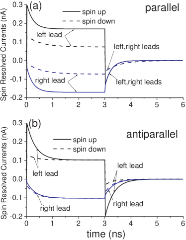
Figure 3: Spin resolved currents against time for both left and right leads and both alignments. In both configurations the currents in the left (right) lead are suppressed (enhanced) just after the voltage is turned on, and then they attain stationary plateaus. When the bias voltage is turned off ($t>3$ns) the left and right currents become the same for each spin component in the P configuration, while in the AP case the $\uparrow$ current becomes bigger than the $\downarrow$ current in the left lead.

In Figure 2(b) we show the evolution of the occupations and the spin accumulation in the antiparallel alignment. We note that $n_{\uparrow}$ increases faster than $n_{\downarrow}$ as in the P case. In contrast, though, $n_{\uparrow}$ attains a higher value than $n_{\downarrow}$ in the stationary regime. This is related to the out-tunnel rates which are now inverted with respect to the parallel case: $\Gamma_{\uparrow}^{R}<\Gamma_{\downarrow}^{R}$. When the bias is turned off both $n_{\uparrow}$ and $n_{\downarrow}$ decrease due to the transient discharge. In particular the spin up electron population discharges predominantly to the left lead while the spin down component discharges to the right, following their corresponding majority density of states (or equivalently the majority tunnel rates). The way how spins $\uparrow$ and $\downarrow$ charge and discharge are more clearly seen in the spin-resolved current curves described in the next section.

III.3 Spin-resolved currents

Figure 3 shows $I_{\uparrow}$ and $I_{\downarrow}$ for both leads and both ferromagnetic alignments. In the P configuration [Fig. 3(a)] the left currents $I_{\uparrow}^{L}$ and $I_{\downarrow}^{L}$ show a transient suppression and then attain their respective stationary values with $I_{\uparrow}^{L}>I_{\downarrow}^{L}$. In the right lead the currents $I_{\uparrow}^{R}$ and $I_{\downarrow}^{R}$ increase (in modulus) up to their respective stationary values. When the bias voltage is turned off $I_{\sigma}^{L}$ becomes negative as $I_{\sigma}^{R}$. The negative sign of both $I_{\sigma}^{L}$ and $I_{\sigma}^{R}$ means that the electrons are flowing from the dot to the leads (discharge). In particular the spin $\downarrow$ electrons discharge much slower than the $\uparrow$ ones, due to $\Gamma_{\downarrow}^{L,R}<\Gamma_{\uparrow}^{L,R}$.

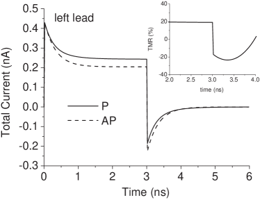
Figure 4: Total current in the left ferromagnetic lead, $I_{\uparrow}^{L}+I_{\downarrow}^{L}$, for both parallel (solid line) and antiparallel (dotted line) configurations. After the bias voltage is turned off ($t>3$ ns) the total antiparallel current becomes greater than the parallel one, lifted by the spike of $\uparrow$ current seen in Fig. 3(b). This results in the time-dependent negative TMR seen in the inset.

In the AP configuration [Fig. 3(b)] $I_{\uparrow}^{L}$ and $I_{\downarrow}^{L}$ show a suppression just after the bias voltage is turned on, then they attain a stationary value with $I_{\uparrow}^{L}=I_{\downarrow}^{L}$. In the right lead the currents $I_{\uparrow}^{R}$ and $I_{\downarrow}^{R}$ are enhanced until they reach equal plateaus. When the bias voltage is turned off, $I_{\uparrow}^{L}$ and $I_{\downarrow}^{L}$ change sign (discharge of the dot) and a spike of spin $\uparrow$ current in seen in the left lead ($I^{L}_{\uparrow}\gg I^{L}_{\downarrow}$). This reflects the preferential discharge of spin up electrons to the left lead, according to $\Gamma_{\uparrow}^{L}>\Gamma_{\uparrow}^{R}$. No spike is seen in the parallel configuration, where spin up electrons discharge equally to both leads. In contrast, in the AP alignment the spin down electrons discharge preferentially to the right lead due to the inverted inequality $\Gamma_{\downarrow}^{L}<\Gamma_{\downarrow}^{R}$, while in the P case its discharge is equally to both sides ($\Gamma_{\downarrow}^{L}=\Gamma_{\downarrow}^{R}$).

Negative TMR. In figure (4) we show the total current in the left lead ($I_{\uparrow}^{L}+I_{\downarrow}^{L}$) for both parallel and antiparallel configurations. Due to the strong spin-polarized discharge ($t>3$ ns) in the left lead when the system is AP aligned, the total current obeys the unusual inequality $I_{AP}^{L}>I_{P}^{L}$, which results in time-dependent negative tunnel magnetoresistance (see inset), defined as $TMR=(I_{P}^{L}-I_{AP}^{L})/I_{AP}^{L}$. As the time evolves the TMR keeps increasing, due to the longer spin-down lifetimes when the system is parallel aligned. More specifically, in the AP configuration both spin up and down discharge fast to the left and to the right leads, respectively, following their majority spin populations (or equivalently the tunneling rates). In contrast, in the P alignment the majority populations occur for spin up in both leads ($\Gamma_{\uparrow}^{L,R}>\Gamma_{\downarrow}^{L,R}$). This turns into a fast discharge for spin up electrons and a slow discharge for the down component. This slow spin down discharge sustains the total current much longer than in the AP configuration, and eventually for long enough times we find $I_{P}^{L}\gg I_{AP}^{L}$.

Displacement Current. In the transient regime the left and the right currents are not in general the same ($I_{L}\neq I_{R}$), due to charge accumulation/depletion in the dot. The generalized conservation law is given by the continuity equation $I^{L}_{\sigma}+I^{R}_{\sigma}-I^{dis}_{\sigma}=0$, where $I^{dis}_{\sigma}$ is the displacement current for spin $\sigma$, given by $I^{dis}_{\sigma}=ed\langle n_{\sigma}(t)\rangle/dt$. In order to check the accuracy of our numerical calculation we have verified numerically the continuity equation.

III.4 Effects of Coulomb Interaction

An exact treatment of the Coulomb interaction represents a formidable problem, and in the context of the present Hamiltonian only few results are known in equilibrium, and none in nonequilibrium, even less so under transient conditions. Nevertheless, in certain limits approximate treatments may give a good qualitative understanding of the generic behavior. One such case is the sequential-tunneling limit ($\Gamma_{0}\ll k_{B}T$), where the Master Equation (ME) approach is known to work well. Here, we use the ME to estimate the effects of Coulomb interaction in our results.timedepenU The current expression is given bymastereq

$$I_{\sigma}^{\eta}=e\Gamma_{\sigma}^{\eta}[f_{\eta}P_{0}-(1-f_{\eta})P_{\sigma}+\tilde{f}_{\eta}P_{\bar{\sigma}}-(1-\tilde{f}_{\eta})P_{2}],$$ (11)

where $P_{0}=\langle(1-n_{\uparrow})(1-n_{\downarrow})\rangle$, $P_{\sigma}=\langle n_{\sigma}(1-n_{\bar{\sigma}})\rangle$ and $P_{2}=\langle n_{\uparrow}n_{\downarrow}\rangle$, are the probabilities to have no electron, one electron with spin $\sigma$ and two electrons, respectively. The Fermi functions $f_{\eta}$ and $\tilde{f}_{\eta}$ are evaluated at $\epsilon_{d}$ and $\epsilon_{d}+U$, respectively. For the dot’s occupation we write

$$\frac{d}{dt}\langle n_{\sigma}\rangle = \frac{1}{e}(I_{\sigma}^{L}+I_{\sigma}^{R})$$ (12)

$$= \sum_{\eta}\Gamma_{\sigma}^{\eta}[f_{\eta}P_{0}-(1-f_{\eta})P_{\sigma}$$

$$+\tilde{f}_{\eta}P_{\bar{\sigma}}-(1-\tilde{f}_{\eta})P_{2}],$$

and for the double occupancy probability we have

$$\frac{d}{dt}\langle n_{\uparrow}n_{\downarrow}\rangle=\sum_{\sigma\eta}\Gamma_{\sigma}^{\eta}[\tilde{f}_{\eta}P_{\bar{\sigma}}-(1-\tilde{f}_{\eta})P_{2}].$$ (13)

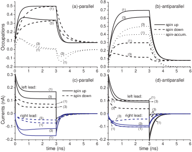
Figure 5: Spin-resolved occupations (a)-(b) and currents (c)-(d) in both parallel (P) and antiparallel (AP) configurations. We take $U=1$ meV and $U=3$ meV, labeling the traces by (1) and (3), respectively. For $U=1$ meV the results are indistinguishable from the $U=0$ case. For $U=3$ meV, though, we find a suppression of the spin-resolved occupations and currents. In the AP alignment this suppression results in an enhancement of the spin accumulation and in a spin polarized current in the stationary plateaus ($|I_{\uparrow}^{L,R}|>|I_{\downarrow}^{L,R}|$). To clarify the range $t>3$ ns, in panel (c) the currents $I_{\sigma}^{L}$ are on top of $I_{\sigma}^{R}$ while in panel (d) they are apart from each other. In addition in the AP case, $|I_{\uparrow}^{L}|$ and $|I_{\uparrow}^{R}|$ for $U=1$ meV are slightly greater than their corresponding values for $U=3$ meV, and $I_{\downarrow}^{R}$ is almost on top of $I_{\uparrow}^{R}$.

For the noninteracting case ($U=0$) the time-dependent results obtained from Eq. (11) are identical to those seen in Sec. III(b)-(c). For the interacting case ($U\neq 0$), we find that for $U=1$ meV the results are indistinguishable from the $U=0$ case [see Fig. 5]. This is so because for small enough $U$ both channels $\epsilon_{d}$ and $\epsilon_{d}+U$ attain resonance for $V(t)=5$ meV. In contrast, for $U=3$ meV the channel $\epsilon_{d}+U$ remains above the emitter chemical potential when the bias voltage is applied, which turns into a suppression of the occupations and the currents. In particular in the AP configuration this suppression is stronger upon the spin down component, seen in both occupations [panel (b)] and currents [panel (d)]. This is due to the spin imbalance $n_{\uparrow}>n_{\downarrow}$ typically present in the antiparallel alignment. This spin-polarized suppression in the AP configuration gives rise to an enhancement of the spin imbalance [see Fig. 5(b)] and to a spin polarized current $(|I_{\uparrow}^{L,R}|>|I_{\downarrow}^{L,R}|)$ in the stationary plateau.

In Fig. (6) we see the effects of $U$ on the dynamical TMR. For $U=1$ meV the TMR is basically the same as before [Fig. 4(inset)]. For $U=3$ meV the TMR is enhanced (in modulus) for both on and off voltage regimes ($0<t<3$ ns and $t>3$ ns, respectively). In particular the Coulomb interaction turns the TMR even more negative after the bias voltage is turned off, which reaches $-40$ % around $3.5$ ns for $U=3$ meV.

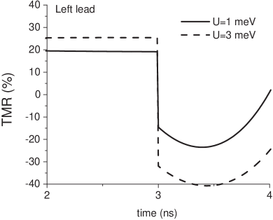
Figure 6: Tunnel magnetoresistance (TMR) as a function of time for $U=1$ and $U=3$ meV. For $U=3$ meV the TMR is enhanced in the stationary regime (2$<t<$3 ns) and becomes even more negative after the bias voltage is turned off ($t>3$ ns).

IV Conclusion

We predict novel spin-dependent effects in a quantum dot coupled to two ferromagnetic leads driven by a rectangular bias voltage pulse. Based on nonequilibrium Green function and master equation techniques we calculated the spin-resolved occupations and currents, the spin accumulation and the tunnel magnetoresistance in the transient just after the bias voltage is turned on and off. Our main findings are: (i) a sign change of the spin accumulation as the time evolves in the P configuration, (ii) a spike of spin $\uparrow$ current in the emitter lead when the system is antiparallel aligned, and (iii) a time-dependent TMR that attains negative values. This negative amount can be further enhanced due to intradot Coulomb interaction.

The authors acknowledge J. C. Egues and J. M. Elzerman for helpful discussions. APJ is grateful to the FiDiPro program of the Finnish Academy for support during the final stages of this work. RMG acknowledges support from CAPES.

References

- (1) Semiconductor Spintronics and Quantum Computation, eds. D. D. Awschalom, D. Loss, and N. Samarth, Springer, Berlin (2002).
- (2) I. Zutic, J. Fabian, and S. Das Sarma, Rev. Mod. Phys. 76, 323 (2004).
- (3) S. A. Wolf, D. D. Awschalom, R. A. Buhrman, J. M. Daughton, S. von Molnár, M. L. Roukes, A. Y. Chtchelkanova, and D. M. Treger, Science 294, 1488 (2001).
- (4) G. A. Prinz, Science 282, 1660 (1998).
- (5) D. P. DiVincenzo, Science 270, 255 (1995); M. A. Nielsen and I. L. Chuang, Quantum Computation and Quantum Information, Cambridge Univ. Press, Cambridge (2000).
- (6) D. Loss and D. P. DiVincenzo, Phys. Rev. A 57, 120 (1998).
- (7) H.-A. Engel and D. Loss, Science 309, 586 (2005); J. C. Egues, Science 309, 565 (2005).
- (8) T. Hayashi, T. Fujisawa, H. D. Cheong, Y. H. Jeong, and Y. Hirayama, Phys. Rev. Lett. 91, 226804 (2003).
- (9) J. M. Elzerman, R. Hanson, L. H. Willems van Beveren, B. Witkamp, L. M. K. Vandersypen, L. P. Kouwenhoven, Nature 430, 431 (2004).
- (10) M. Kroutvar, Y. Ducommun, D. Heiss, M. Bichler, D. Schuh, G. Abstreiter, and J. J. Finley, Nature 432, 81 (2004).
- (11) R. Hanson, L. H. W. Beveren, I. T. Vink, J. M. Elzerman, W. J. M. Naber, F. H. L. Koppens, L. P. Kouwenhoven, and L. M. K. Vandersypen, Phys. Rev. Lett. 94, 196802 (2005).
- (12) F. H. L. Koppens, C. Buizert, K. J. Tielrooij, I. T. Vink, K. C. Nowack, T. Meunier, L. P. Kouwenhoven, and L. M. K. Vandersypen, Nature 442, 766 (2006).
- (13) L. P. Kouwenhoven, J. M. Elzerman, R. Hanson, L. H. Willems van Beveren, and L. M. K. Vandersypen, Phys. Stat. Sol. (b) 243, 3682 (2006).
- (14) J. Splettstoesser, M. Governale, J. König, F. Taddei, and R. Fazio, Phys. Rev. B 75, 235302 (2007).
- (15) E. Sela and Y. Oreg, Phys. Rev. Lett. 96, 166802 (2006).
- (16) E. Cota, R. Aguado, and G. Platero, Phys. Rev. Lett. 94, 107202 (2005).
- (17) L. Arrachea, Phys. Rev. B 72, 125349 (2005).
- (18) M. Switkes, C. M. Marcus, K. Campman, and A. C. Gossard, Science 283, 1905 (1999).
- (19) R. López, D. Sánchez, and G. Platero, Phys. Rev. B 67, 035330 (2003).
- (20) A. Kaminski, Y. V. Nazarov, and L. I. Glazman, Phys. Rev. B 62, 8154 (2000).
- (21) R. López, R. Aguado, G. Platero, and C. Tejedor, Phys. Rev. Lett. 81, 4688 (1998).
- (22) R. López, R. Aguado, G. Platero, and C. Tejedor, Phys. Rev. B 64, 075319 (2001).
- (23) Y. Yu, T. C. Au Yeung, W. Z. Shangguan, and C. H. Kam, Phys. Rev. B 63, 205314 (2001).
- (24) Z. -G. Zhu, G. Su, Q. -R. Zheng, B. Jin, Phys. Rev. B 70, 174403 (2004).
- (25) C. Lui, B. Wang, and J. Wang, Phys. Rev. B 70, 205316 (2004).
- (26) C. -C. Kaun and T. Seideman, Phys. Rev. Lett. 94, 226801 (2005).
- (27) F. J. Kaiser, P. Hänggi, and S. Kohler, European Physical Journal B 54, 201 (2006).
- (28) L. Arrachea, Phys. Rev. B 70, 155407 (2004).
- (29) K. M. Fonseca-Romero, S. Kohler, and P. Hänggi, Phys. Rev. Lett. 95, 140502 (2005).
- (30) A. P. Jauho and K. Johnsen, Phys. Rev. Lett. 76, 4576 (1996).
- (31) Y. Utsumi, J. Martinek, G. Schön, H. Imamura, and S. Maekawa, Phys. Rev. B 71, 245116 (2005).
- (32) J. Martinek, Y. Utsumi, H. Imamura, J. Barnaś, S. Maekawa, J. König, and G. Schön, Phys. Rev. Lett. 91, 127203 (2003).
- (33) F. M. Souza, J. C. Egues, and A. P. Jauho, Phys. Rev. B 75, 165303 (2007).
- (34) I. Weymann, J. Barnaś, J. König, J. Martinek, and G. Schön, Phys. Rev. B 72, 113301 (2005).
- (35) I. Weymann and J. Barnaś, Phys. Rev. B 73, 33409 (2006); J. Barnaś and A. Fert, Phys. Rev. Lett. 80, 1058 (1998).
- (36) J. Varalda, A. J. A. de Oliveira, D. H. Mosca, J. -M. George, M. Eddrief, M. Marangolo, and V. H. Etgens, Phys. Rev. B 72, 81302(R) (2005).
- (37) A. Brataas, Y. V. Nazarov, J. Inoue, and G. E. W. Bauer, Phys. Rev. B 59, 93 (1999); H. Imamura, S. Takahashi, and S. Maekawa, Phys. Rev. B 59, 6017 (1999); J. Martinek, J. Barnaś, S. Maekawa, H. Schoeller, and G. Schön, Phys. Rev. B 66, 014402 (2002).
- (38) A. P. Jauho, N. S. Wingreen, and Y. Meir, Phys. Rev. B 50, 5528 (1994).
- (39) H. Haug and A. P. Jauho, Quantum Kinetics in Transport and Optics of Semiconductors, Springer Solid-State Sciences 123 (1996).
- (40) The wideband limit consists of (i) neglecting the real part of the tunneling self-energy (level-shift), (ii) assuming that the line-widths are energy independent constants, and (iii) allowing a single time dependence, , for the energies in each lead [hh96, ].
- (41) For an analysis that does not rely on the wideband limit see J. Maciejko, J. Wang, and H. Guo, Phys. Rev. B 74, 085324 (2006).
- (42) The spin-independent version of this expression was originally obtained in N. S. Wingreen, A. P. Jauho, and Y. Meir, Phys. Rev. B 48, 8487(R) (1993).
- (43) W. Rudziński and J. Barnaś, Phys. Rev. B 64, 85318 (2001).
- (44) In the present work , i.e., we are at the sequential tunneling limit, so no coherent oscillations in the current are observed as in previous works [apj94, ],[nsw93, ].
- (45) Typical values for and in quantum dot systems can be seen, for instance, in D. Goldhaber-Gordon, J. Göres, M. A. Kastner, H. Shtrikman, D. Mahalu, and U. Meirav, Phys. Rev. Lett. 81, 5225 (1998); F. Simmel, R. H. Blick, J. P. Kotthaus, W. Wegscheider, and M. Bichler, ibid. 83, 804 (1999); D. G.-Gordon, H. Shtrikman, D. Mahalu, D. A.-Magder, U. Meirav, M. A. Kastner, Nature 391, 156 (1998).
- (46) For an experimental setup to measure TMR in the presence of short voltage pulses, ranging from 0.5 to 500 ns, we address the reader to K. B Klaassen, X. Xing, and J. C. L. van Peppen, IEEE Trans. Mag. 40, 195 (2004).
- (47) The effect of Coulomb interaction on time-dependent transport has been previously studied, e.g., by Q. Sun, J. Wang, and T. Lin, Phys. Rev. B 58, 13007 (1998), and also in Ref. [rl01, ] and Ref. [yy01, ].
- (48) L. I. Glazman and K. A. Matveev, JEPT Lett.48, 445 (1988); H. Bahlouli, Phys. Stat. Sol. (a) 179, 475 (2000).