Statistics of Core Lifetimes in Numerical Simulations of Turbulent, Magnetically Supercritical Molecular Clouds

Abstract

We present measurements of the mean dense core lifetimes in numerical simulations of magnetically supercritical, turbulent, isothermal molecular clouds (MCs), in order to compare with observational determinations. The mean “prestellar” lifetimes are given as a function of the mean density within the cores, which in turn is determined by the density threshold $n_{\rm thr}$ used to define them. The mean lifetimes are consistent with observationally reported values, ranging from a few to several free-fall times. We also present estimates of the fraction of cores in the “prestellar”, “stellar”, and “failed” stages as a function of $n_{\rm thr}$. Failed cores are defined as those that do not manage to collapse, but rather re-disperse back into the environment. Due to resolution limitations, the number ratios are measured indirectly in the simulations, as either lifetime ratios (for the prestellar cores), or as time-weighted mass ratios (for the failed cores). Our approach contains one free parameter, the lifetime of a protostellar object $\tau_{\rm yso}$ (Class 0 + Class I stages), which is outside the realm of the simulations. Assuming a value $\tau_{\mathrm{yso}}=0.46$ Myr, we obtain number ratios of starless to stellar cores ranging from 4–5 at $n_{\rm thr}=1.5\times 10^{4}{\rm~{}cm}^{-3}$ to $\sim 1$ at $n_{\rm thr}=1.2\times 10^{5}{\rm~{}cm}^{-3}$, again in good agreement with observational determinations. We also find that the failed cores are generally difficult to detect, although the mass in these cores is comparable to that in stellar cores at $n_{\rm thr}=1.5\times 10^{4}{\rm~{}cm}^{-3}$. At $n_{\rm thr}=1.2\times 10^{5}{\rm~{}cm}^{-3}$ the mass in failed cores is negligible, in agreement with recent observational suggestions that at the latter densities the cores are in general gravitationally dominated. We conclude by noting that the timescale for core contraction and collapse is virtually the same in the subcritical, ambipolar diffusion-mediated model of star formation, in the model of star formation in turbulent supercritical clouds, and in a model intermediate between the previous two, suggesting a convergence of the models at least at the level of the core lifetimes, for currently accepted values of the clouds’ magnetic criticality.

1 Introduction

The evolution of the dense cores within molecular clouds (MCs) on their route to forming stars, and the duration of the various stages of contraction and collapse in particular, are key ingredients in our understanding of the star formation process. The process of contraction and final collapse of a core is generally divided in the so-called “prestellar” phase, which includes the span between the time when the core is first detected and when a protostellar object forms in its deepest regions, and the “stellar” phase, which includes the Class 0 and Class I protostellar stages (from the appearance of the protostellar object to the clearance of the surrounding material).

Observationally, several works have estimated the duration of the prestellar stage through either statistical or chemical methods (see the discussion in Ballesteros-Paredes et al., 2007, and references therein). The former rely on measuring the number ratio of prestellar to stellar cores, and assuming that this ratio equals the ratio of durations of these stages (e.g., Beichman et al., 1986; Lee & Myers, 1999; Onishi et al., 2002; Hatchell et al., 2007; J$\o$rgensen et al., 2007). A summary of prestellar durations, or “lifetimes”, from several studies, has been recently presented by Ward-Thompson et al. (2007).

Theoretically, there are two main competing models that describe the evolution of the cloud cores. The so-called “standard model” of quasi-static contraction mediated by ambipolar diffusion (AD; e.g., Mouschovias, 1976, 1991; Shu et al., 1987) was the dominant paradigm until recently. It postulated that the cores in low-mass star-forming regions evolved quasi-statically in magnetically subcritical clouds, contracting gravitationally at the rate allowed by AD, which causes a redistribution of the magnetic flux, until the central parts of the cores become magnetically supercritical and proceed to dynamical collapse. The process was originally thought to be slow, because the clouds were thought to be strongly magnetically subcritical, in which case the AD timescale $\tau_{\rm AD}$ is roughly one order of magnitude larger than the free-fall time. However, it was later recognized that near-magnetically critical initial conditions (Fiedler & Mouschovias, 1993; Ciolek & Basu, 2001) or turbulent conditions (Fatuzzo & Adams, 2002; Heitsch et al., 2004) cause the AD timescale to become significantly shorter, only a few times longer than the free-fall time (Ciolek & Basu, 2001; Vázquez-Semadeni et al., 2005a, hereafter Paper I). This realization was motivated in part by observational studies suggesting core lifetimes not much longer than their free-fall times (e.g., Lee & Myers, 1999; Jijina et al., 1999). A recent numerical study of core lifetimes dominated by AD but with turbulent initial conditions has been presented recently by Nakamura & Li (2005), finding core lifetimes in the range 1.5–10 times the free-fall time.

On the other hand, the so called “turbulent” model of star formation (e.g., Ballesteros-Paredes et al., 1999a; Vázquez-Semadeni et al., 2000; Mac Low & Klessen, 2004; Ballesteros-Paredes et al., 2007) takes into account the fact that MCs are turbulent, and attributes a dual character to the turbulence: on the one hand it provides support against generalized cloud collapse, but on the other it produces strong local density enhancements, which constitute the clumps and cores within the clouds. Thus, their formation timescales are of the order of the turbulent crossing time across the size scales of the fluid parcels that collide to produce the clumps and cores (Ballesteros-Paredes et al., 1999b; Elmegreen, 2000; Padoan & Nordlund, 2002). However, Paper I showed that the lifetimes of randomly selected cores at densities comparable to those of observed ammonia cores are nevertheless of the order of a few times the free-fall time of the cores, because their evolution while they are detectable includes part of the assembly process and then the collapsing stage. Note that this is contrary to frequent perceptions that the turbulent model implies core lifetimes of approximately one free-fall time (e.g., Ward-Thompson et al., 2007).

Within the context of the turbulent model, it is natural to expect the existence of an additional class of MC clumps that end up redispersing rather than collapsing; that is, turbulent density fluctuations that do not manage to become locally gravitationally unstable (Elmegreen 1993; Taylor et al. 1996; Paper I). We refer to these as “failed” clumps. Also, in this model, it is not crucial whether the clouds are magnetically subcritical or supercritical, since much of the “filtering” of mass that reaches the collapsed objects, and which regulates the star formation efficiency, is provided by the dual role of the turbulence. A stronger magnetic field simply appears to provide an extra reduction factor for the star formation efficiency, whose precise magnitude depends on whether the turbulence in the clouds is driven or decaying (see the discussion in Vázquez-Semadeni, 2007, and references therein).

In this paper we present a survey of the core lifetimes in a set of numerical simulations of a turbulent, continuously driven, magnetically supercritical, isothermal MC, with the aim of obtaining statistically reliable data about them within this model, that can be compared to observational determinations. We also discuss the number ratio of “starless” to “stellar” (in the simulations, collapsed) cores. The plan of the paper is as follows: In §2 we describe the numerical simulations we analyzed; in §3 we describe the method we used to measure the lifetimes and the number ratios of the various kinds of objects; in §4 we compare them with existing observational and theoretical work, and discuss their implications. In this section we also discuss the limitations and accomplishments of the present work.

2 The Numerical Simulations

We have chosen the moderately supercritical simulation (named M10J4$\beta$.1) reported in Paper I for analysis of the core evolution. We refer to this run as “R1” in the rest of the paper, and its selection was based on the fact that observations suggest that MCs are nearly critical or moderately supercritical (Crutcher, 1999). The computational domain contained 64 Jeans masses, or 1860 $M_{\odot}$ (Vázquez-Semadeni et al., 2005b). The mean number density is $n_{0}=500{\rm~{}cm}^{-3}$, the simulation box size is 4 pc, and the (uniform) temperature is $T=11.4$ K, so that the sound speed is $c_{\rm s}=0.2{\rm~{}km~{}s}^{-1}$. The mean magnetic field was $B_{0}=14.5~{}\mu$G, giving a mass-to-magnetic-flux ratio $\mu=2.8$ times the critical value. These physical properties and conditions of the simulation make it directly comparable to the most massive “supercores” in the Perseus cloud, as defined by Kirk et al. (2006). Indeed, supercore No. 2 (IC 348) is reported by those authors to have a mass $\sim 1940~{}M_{\sun}$, and, at a distance of 250 pc, its size is $\sim 5$ pc, very close to the corresponding parameters of our simulation. Supercore No. 7 (NGC 1333) is reported to be somewhat smaller and less massive, at $\sim 970~{}M_{\sun}$.

The turbulence in this simulation was continuously driven in order to maintain a turbulent Mach number $\sim 10$. For the turbulence random driver, we follow the method in Stone et al. (1998), i.e., we applied a random Fourier driver operating at the largest scales with the functional form $P(k)\propto k^{6}\exp{(-8k/k_{\rm peak})}$, where $k=2\pi/l$ is the wavenumber corresponding to the scale $l$, $k_{\rm peak}=2(2\pi/L)$ is the wavenumber where the input power spectrum peaks, and $L$ is the one-dimensional size of the computational box. As discussed in Paper I, this is motivated by the fact that turbulence is ubiquitous at all scales in molecular clouds (e.g., Larson, 1981; Blitz, 1993; Heyer & Brunt, 2004), including starless ones such as the so-called Maddalena’s cloud (Maddalena & Thaddeus, 1985), which suggests a universal origin and maintenance mechanism for the clouds’ turbulence, and that turbulence is driven at the largest scales in the clouds (Heyer & Brunt, 2004, 2007).

Two more simulations (called R2 and R3) were performed with the same physical parameters but different random seeds for the Fourier driver. R2 was performed at a resolution of 256 cells per dimension, and R3 was performed at 512 cells per dimension. We used a total variation diminishing (TVD) scheme (Kim et al., 1999). Runs R1 and R2 were integrated over 10 Myr, before self-gravity was turned on (5 turbulent crossing times). This is a standard procedure aimed at allowing the system to attain a well-developed, stationary turbulent state by the time gravity is turned on, thus preventing it from “capturing” features produced directly by the artificial random driver. Note that, however, one turbulent crossing time is generally enough to achieve such a stationary state (Ballesteros-Paredes et al., 2006). Thus, run R3 (the more expensive of these simulations in terms of computational time) was run only for one dynamical time before self-gravity was turned on.

Once self-gravity was turned on, runs R1, R2 and R3 were integrated over 13, 9.1, and 4.7 Myr respectively. In reality, however, as suggested by the estimated ages of the stellar population in the Solar Neighborhood (Ballesteros-Paredes et al., 1999b; Hartmann et al., 2001; Ballesteros-Paredes & Hartmann, 2007), molecular clouds should live not much longer than 5 Myr, since they are destroyed by stellar winds, bipolar outflows, SNe explotions, etc. For this reason, we only used the first 8 Myr of the evolution of runs R1 and R2 with self-gravity.

Note that run R1 was used to perform the analysis over all types of cores (collapsed and failed). However, since only two collapse events were found in R1, we used runs R2 and R3 to verify that the timescales for formation and collapse obtained in R1 were consistent, and independent of the resolution. Run R2 produced two collapse events, while run R3 produced three.

3 Measurement procedure

3.1 General considerations

Just as with observations, estimating the core lifetimes in the simulations is not a straightforward task. The numerical simulations have both advantages and disadvantages compared to the observations. First, in the simulations, the density, velocity and magnetic fields defined over the three spatial and one temporal dimensions are given. However, the cores, defined as we describe below, are elusive entities that in general do not preserve their identity over time; i.e., they do not involve the same mass at different times. After all, defining a core amounts to defining a certain region of space in what is really a fluid continuum. We choose to define a core as the set of connected grid cells surrounding a local density peak and having densities above a given density threshold $n_{\rm thr}$. This definition mimics the emission observed when using tracers sensitive to different density regimes. We have chosen not to use an algorithm such as CLUMPFIND (Williams et al., 1994) because it can sometimes introduce artificial divisions across mostly continuous objects. Our chosen definition allows large-scale clumps to be defined at low $n_{\rm thr}$ even if the region contains more than one local density maximum.

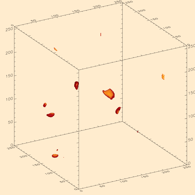
Figure 1: Cores defined at $n_{\rm thr}=30~{}n_{0}=1.5\times 10^{4}{\rm~{}cm}^{-3}$, and at $t=1.96$ Myr for R1. This time marks the end of collapse for the first collapsing core (the biggest core seen near the center of the simulation box) in this run. At this threshold, failed cores become an important feature and many of them coexist at every temporal step. The two “spots” at opposite sides of the $y$-axis boundaries, and at $(x,z)=(203,197)$ correspond to just one failed core crossing the periodic boundaries. An animation of the simulation for $0.32\leq t/\mathrm{Myr}\leq 8$ is presented in the electronic version of the Journal, with the frames separated by $\Delta t=0.04$ Myr. The first 9 frames are omitted, since there are no structures above $n_{\rm thr}$ at those times. The figure shown in the printed version of the Journal corresponds to frame #40 in the animation.

In general, the cores are more poorly defined as lower values of $n_{\rm thr}$ are considered, while instead this problem disappears as one considers higher $n_{\rm thr}$. Once defined, the cores must be followed over time. The animation of R1 associated to Fig. 1 in the electronic edition shows the evolution of the cores when $n_{\rm thr}=30~{}n_{0}=1.5\times 10^{4}{\rm~{}cm}^{-3}$, illustrating how the failed cores appear and disappear, and sometimes merge or split. It also illustrates a merger of collapsing cores (cf. §3.2). The measured core properties (e.g., volume $V$, mass $m$, and mean density $\bar{n}$) depend on $n_{\rm thr}$, and furthermore, at a fixed value of $n_{\rm thr}$, these properties vary in time for every core. Note in particular that the cores are not generally composed of the same fluid parcels throughout their history. Peak densities and their associated coordinates within a core do not depend on $n_{\rm thr}$, which only defines the time at which these two properties begin to be measured.

The cores in the simulations can either collapse or rebound (no stable hydrostatic solutions are possible in the isothermal, magnetically supercritical regime; see Paper I). Thus, there exist two classes of starless cores: those that are on route to collapse, to which we refer as “prestellar”, and those that will eventually redisperse back to the surrounding medium, to which we refer as “failed” cores. In addition, we refer to cores that have already collapsed as “stellar”. With these considerations in mind, we see that the number ratio of starless to stellar cores is given by

$$\frac{N_{\star\mathrm{less}}}{N_{\star}}=\frac{N_{\mathrm{pre}}}{N_{\star}}+\frac{N_{\mathrm{f}}}{N_{\star}},$$ (1)

where $N_{\star\mathrm{less}}$, $N_{\rm pre}$, $N_{\star}$ and $N_{\rm f}$ are respectively the numbers of starless, prestellar, stellar and failed cores.

Our goal in the present paper is to determine the lifetimes of the cores and their number ratios as a function of the threshold used to define them or, almost equivalently, as a function of their mean densities. The lifetimes that are reported in observational studies correspond to the duration of the prestellar stage, and are normally estimated by measuring the number of cores in the prestellar and stellar stages, and assuming that the ratio of their numbers equals the ratio of their durations. However, it was shown in Paper I that the ratio of the numbers is an upper limit to the ratio of durations if there exists a population of failed cores that is not accounted for. Furthermore, as discussed in Ballesteros-Paredes & Hartmann (2007), potential source count incompleteness in several observational surveys also contributes to make this an upper limit.

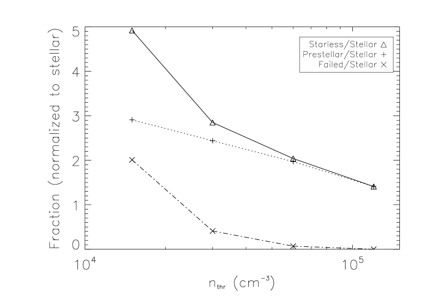
Figure 4: Left panel: Number ratios of the stellar (dashed line, diamonds), total starless (solid line, triangles), prestellar (dotted line, plus signs) and failed (dash-dotted line, crosses) cores. Right panel: Number ratios of the total starless, prestellar and failed cores (same lines and symbols as in the left panel), normalized to the number of stellar cores.

In principle, one could simply measure the numbers of the various types of cores (failed, prestellar and stellar) in the simulations. However, a number of limitations prevent us from doing so. We have found that the collapsed, or stellar, cores in our simulations are clearly under-resolved. Their masses are typically between 50 and 100 $M_{\sun}$, while the smallest and densest cores in, e.g., Perseus, have masses $\sim 1M_{\sun}$, although they are clustered in groups of up to several tens of them (see, for example, Figs. 4 and 5 of Kirk et al., 2006). Specifically, we have extracted the masses of the clustered submillimeter (submm) cores in supercore No. 2 and supercore No. 7 from tables 1, 2 and 3 of Kirk et al. (2006). We find a total mass in these clustered submm cores of $\sim 7~{}M_{\sun}$ for supercore No. 2 and $\sim 32~{}M_{\sun}$ for supercore No. 7. In comparison, the masses at the time of peak density saturation of each of the collapsed objects in R1 at $n_{\rm thr}=1.2\times 10^{5}{\rm~{}cm}^{-3}$ (emulating the density of the submm cores) are $61~{}M_{\sun}$ and $62~{}M_{\sun}$ respectively. Thus, each of our cores with collapsed objects corresponds most directly to a cluster of protostellar cores.

Another important issue is that the number of objects fluctuates statistically in time. This suggests that we should consider appropriately weighted time averages in order to obtain the most representative numbers. As mentioned, our analysis in R1 was performed over the first 8 Myr of the simulation after gravity was turned on, except for the failed cores at the lowest $n_{\rm thr}$, for which a sufficiently large statistical sample was obtained considering only the first 4 Myr (due to the large number of these objects). Analysis in R2 and R3 consisted only of collapse time measurements taken over 8 Myr and 5 Myr (the duration of R3) after gravity is turned on respectively.

The time interval between outputs in the simulations was 0.04 Myr, and we used four different values of the density threshold: $n_{\rm thr}=1.5\times 10^{4},~{}3\times 10^{4},~{}6\times 10^{4},$ and $1.2\times 10^{5}{\rm~{}cm}^{-3}$. Higher threshold densities were not used because cores with $n>256~{}n_{0}=1.28\times 10^{5}{\rm~{}cm}^{-3}$ are not well resolved in all the simulations according to the Jeans condition (Truelove et al., 1997), as explained in Paper I. Thresholds lower than $20~{}n_{0}=10^{4}{\rm~{}cm}^{-3}$ were not investigated either, because at such low densities the cores become impossible to follow in time due to their poorly defined identities (see, for example, the animations accompanying Paper I). In the next subsections we describe how we estimate the numbers and lifetimes of the various kinds of cores.

3.2 Collapsing cores

3.2.1 Time scales

When a core collapses in the simulations, in practice its peak density $n_{\rm pk}$ does not increase to infinity, but rather reaches a saturated value $n_{\rm sat}\sim$ 2–3 $\times 10^{6}{\rm~{}cm}^{-3}$ at $256^{3}$ resolution or $n_{\rm sat}\sim$ 1 $\times 10^{7}{\rm~{}cm}^{-3}$ in the $512^{3}$ simulation, beyond which the collapse cannot be followed further by the code. In this state, the mass of the collapsed object is spread out over a few pixels in each direction. This process is illustrated in Fig. 2, which shows the evolution of the peak densities of the objects that collapse in the three runs. Upper, middle and lower panels represent the peak density as a function of time for runs R1, R2, and R3, respectively. The saturated density of a collapsed core in general oscillates in time. This is because the code contains no prescription for “capturing” the mass in the collapsed objects (the analogue of a “sink particle” in SPH codes, for example), and therefore this mass still interacts with its surroundings. Also, $n_{\rm sat}$ increases slowly on average, because the collapsed object continues to slowly accrete mass.

We define the prestellar lifetime of a core, $\tau_{\rm pre}$, as the interval between the time when it is first detected at a given threshold $n_{\rm thr}$, and the time when its peak density reaches the saturated value. This implicitly assumes that any further subfragmentation of the core occurs essentially simultaneously, so that all protostars form at roughly the same time, at least within the precision of our temporal resolution. This definition of the prestellar lifetime neglects the duration of the final stages of collapse (from the time when the density saturates in the simulation to the time at which actual protostellar densities would be reached). This approximation should not introduce a large error, since the free-fall time at the saturation densities is

$$\tau_{\rm ff}\equiv(3\pi/32G\rho)^{1/2}\sim 2\times 10^{4}~{}\hbox{yr},$$ (2)

which is significantly shorter than the temporal resolution of $4\times 10^{4}$ yr between snapshots in our simulation. In any case, this slight underestimate of the true prestellar lifetime acts in the opposite direction of any delay of the collapse introduced by numerical diffusion, and thus the two effects should tend to cancel each other out (see the discussion in §4.2).

The measured prestellar lifetime obviously depends on $n_{\rm thr}$, since this quantity defines the starting time of a core’s observed “life”. Empirically, we have found that the mean density in the cores scales close to linearly with $n_{\rm thr}$ (e.g., Vázquez-Semadeni et al., 1997), and so this means that the measured prestellar lifetime should be a function of the mean density as well, in qualitative agreement with observational data (Ward-Thompson et al., 2007).

We ignore mergers of collapsing cores in the measurement of $\tau_{\rm pre}$. That is, if two cores appear at times $t_{1}$ and $t_{2}>t_{1}$ respectively, and they merge at a later time $t_{3}$ into a new core that eventually collapses, we take the prestellar lifetime $\tau_{\rm pre}$ as the time elapsed between $t_{1}$ and the time of density saturation. We do this motivated by the fact that the peak densities $n_{\rm pk}$ of cores that merge into a new core which collapses later are seen to rise rapidly even before the merging event, suggesting that these cores were already on their own independent route to collapse, rather than the latter being triggered by the merging event. For instance, the first two cores in R1 (upper panel of Fig. 2, solid and dashed lines respectively) are seen to appear at roughly the same time ($t\sim 1.4$ Myr), and to merge shortly thereafter. Thus, we consider them together as the single first collapse event in R1. The third core is seen to have very similar physical properties to those of the merger, and we refer to its collapse as the second collapse event in R1. In Fig. 3 we report the prestellar lifetimes measured for the collapse events in R1 (diamonds), R2 (triangles) and R3 (squares) as a function of their mean densities (which in turn are $\sim n_{\rm thr}$).

It is important to remark that the long durations of the collapsed objects after they have collapsed seen in Fig. 2 does not imply that the stellar cores last that long, because no modeling of stellar energy feedback (e.g., winds, bipolar outflows, ionizing radiation) is included in the numerical model, and thus the cores cannot be dispersed after they produce collapsed objects.

3.2.2 Number ratios

As mentioned in §3.1, we cannot simply count the number of cores with collapsed objects because it is clear that at the resolutions we used their subfragmentation was not appropriately captured. Thus, instead, we proceed inversely to the standard observational procedure, and estimate the number ratio of prestellar to stellar cores simply as the ratio of the prestellar lifetime to the lifetime of the embedded protostellar phase:

$$\frac{N_{\mathrm{pre}}}{N_{\star}}=\frac{\overline{\tau_{\mathrm{pre}}}}{\tau_{\mathrm{yso}}},$$ (3)

where $\overline{\tau_{\mathrm{pre}}}$ is the average of the measured prestellar lifetimes for the seven collapse events in the simulations, and $\tau_{\rm yso}$ is the duration of the protostellar stage. We emphasize that eq. (3) allows us to estimate the number ratio of prestellar to stellar cores, but not the actual numbers, and that this ratio is a function of the threshold density, since $\tau_{\mathrm{pre}}$ is.

For us, $\tau_{\mathrm{yso}}$ is a free parameter because it is outside the realm of our simulations. As mentioned in §3.2.1, no modeling of the feedback from the protostars such as bipolar outflows, ionization radiation or winds is included, so there are no energy sources available for dispersing the cores once they are formed. Thus, we have to consider it as a free parameter in our study, whose value is to be set on the basis of external information.

Observationally, $\tau_{\rm yso}$ is normally estimated by obtaining the ratio of the number of embedded objects to that of the T Tauri stars (e.g., Wilking et al., 1989; Kenyon et al., 1990; Greene et al., 1994; Kenyon & Hartmann, 1995; Hatchell et al., 2007). Values for $\tau_{\mathrm{yso}}$ reported in the literature are $\sim 0.6\pm 0.3$ Myr (see review by Ward-Thompson et al., 2007, and references therein), the spread being due to both observational constraints and real differences among the observed regions.

We take $\tau_{\mathrm{yso}}=0.46$ Myr, the mean value obtained for Perseus by Hatchell et al. (2007). We base this selection on two considerations: First, their estimate of $\tau_{\mathrm{yso}}$ includes corrections for incompleteness of surveys toward very low masses and multiplicity. Second, we have found that our simulations are reasonably resemblant of a massive “supercore” in Perseus, as defined by Kirk et al. (2006) (see §2 and §3.1).

3.3 Failed cores

Failed cores in our simulations are less dense than collapsing cores, and therefore are not as strongly affected by the limited resolution of our simulations. Nevertheless, we consider it safer to estimate their number ratio with respect to the stellar cores through the ratio of masses in these two kinds of objects. This estimator avoids the uncertainty associated with the possible failure to capture further subfragmentation of the cores. However, even this is still not completely straightforward because we need to take into account temporal effects.

The failed cores “appear” at some time and “disappear” at a later time at a given density threshold $n_{\rm thr}$. Furthermore, their masses are continuously varying over this time interval, first increasing, reaching a maximum value, and then decreasing again. In order to obtain an estimator that is most representative of the number ratio expected to be found upon a single instantaneous observation, we take the ratio of the temporal averages of the masses of the failed cores to those of the stellar cores, weighted by the ratio of their typical durations

$$\frac{N_{\mathrm{f}}}{N_{\star}}=\frac{\sum_{i}\langle m_{i}\rangle\tau_{i}}{\tau_{\mathrm{yso}}\sum_{j}\langle m_{j}\rangle},$$ (4)

where the summations over $i$ and $j$ refer to the failed and stellar cores respectively, $\langle m_{i}\rangle$ and $\tau_{i}$ are respectively the time-averaged mass and the duration of the $i$-th failed core, and $\tau_{\rm yso}$ is the duration of the protostellar phase discussed in §3.2. For the stellar cores, we take $\langle m_{j}\rangle$ as the average mass over a time interval $\tau_{\rm yso}$ after the core has collapsed.

Equation (4) assumes that actual failed cores have, on average, the same mass as stellar cores. However, it is reasonable to expect failed cores to be less massive in general than individual stellar cores, and in this case the right-hand side of eq. (4) is a lower limit for the failed-to-stellar core ratio. Furthermore, eq. 4 also assumes that no fragment of a failed core ever ends up collapsing, and no fragment of a stellar core ends up redispersing. This is a reasonable assumption, since subfragmentation of the cores is mostly a gravitational phenomenon, which occurs after the onset of collapse. Thus, collapsing cores are expected to fragment into further collapsing units, while failed cores are not expected to fragment because they do not engage into collapse. In fact, the failed cores in our simulations generally have very small, sub-solar masses (see §4.1).

3.4 The starless to stellar ratio

Equations (3) and (4) give us the prescriptions to estimate the terms on the right-hand side of eq. (1). We can then estimate number ratios with respect to the total number of cores $N_{\mathrm{tot}}=N_{\mathrm{pre}}+N_{\mathrm{f}}+N_{\star}$ in terms of the ratios derived in eqs. (1), (3), and (4) as follows:

$$\frac{N_{\mathrm{pre}}}{N_{\mathrm{tot}}} = \biggl{[}\frac{N_{\star\mathrm{less}}/N_{\star}}{N_{\mathrm{pre}}/N_{\star}}+\biggl{(}\frac{N_{\mathrm{pre}}}{N_{\star}}\biggr{)}^{-1}\biggr{]}^{-1}$$ (5)

$$\frac{N_{\mathrm{f}}}{N_{\mathrm{tot}}} = \biggl{[}\frac{N_{\star\mathrm{less}}/N_{\star}}{N_{\mathrm{f}}/N_{\star}}+\biggl{(}\frac{N_{\mathrm{f}}}{N_{\star}}\biggr{)}^{-1}\biggr{]}^{-1}$$ (6)

$$\frac{N_{\star\mathrm{less}}}{N_{\mathrm{tot}}} = \biggl{[}1+\biggl{(}\frac{N_{\star\mathrm{less}}}{N_{\star}}\biggr{)}^{-1}\biggr{]}^{-1}$$ (7)

$$\frac{N_{\star}}{N_{\mathrm{tot}}} = \biggl{[}1+\frac{N_{\star\mathrm{less}}}{N_{\star}}\biggr{]}^{-1}$$ (8)

These fractions are shown in Fig. 4 (left panel) as a function of $n_{\rm thr}$. The right panel of this figure shows the same ratios but normalized to the number of stellar cores.

4 Discussion

4.1 Comparison with previous work

In addition to the core lifetimes as a function of their mean densities, Fig. 3 shows two lines indicating the locus of $t=\tau_{\rm ff}$ and $t=10\tau_{\rm ff}$, with $\tau_{\rm ff}$ defined in eq. (2). This figure can be compared with Figure 2 of Ward-Thompson et al. (2007). It is seen that, within the uncertainties, the core lifetimes in our simulations are in good agreement with the observational values, being in general a few to several times the free-fall time. However, such a comparison should be taken with care because in the determination of observational lifetimes, the assumed values for $\tau_{\rm yso}$ span one order of magnitude (from $10^{5}$ to $10^{6}$ yr). In any case, one can unambiguously conclude that the prestellar core lifetimes in the turbulent scenario are a few times $\tau_{\rm ff}$, and not only $1\tau_{\rm ff}$ as is often stated in literature (e.g., Kirk et al., 2005; Ward-Thompson et al., 2007).

These results can be understood as a consequence of several factors. First, the cores take some time to be assembled by the external turbulent compressions before they become gravitationally unstable (Gómez et al., 2007), and even after that, some readjustments of the mass and some oscillations are expected to occur before gravitational collapse sets in. Moreover, as pointed out by Larson (1969), the duration of the actual collapse is longer than the free-fall time because the thermal pressure gradient is never negligible. So, even though the cores in the simulation are formed dynamically, their lifetimes are fully consistent with observational estimates.

The number ratio of prestellar to stellar cores in our simulations and the ratio of durations of these stages at low values of $n_{\rm thr}$ are $\sim 3$ (Fig. 4, right panel). The same value is obtained by Lee & Myers (1999), who studied an optically-selected sample of cores, characterized by relatively low mean densities, $\lesssim 10^{4}{\rm~{}cm}^{-3}$. Note, however, that we obtain a number ratio of total starless (prestellar + failed) to stellar cores of $\sim 5$, larger than the observation of Lee & Myers (1999). This suggests that their sample consisted mostly of prestellar cores, possibly because the failed cores tend to be smaller and therefore less easily detected. Indeed, Fig. 5 (left panel) shows a size histogram of the failed cores at $n_{\rm thr}=30~{}n_{0}=1.5\times 10^{4}{\rm~{}cm}^{-3}$ for R1, and it can be seen that virtually all of them have sizes $\ell<0.2$ pc, with $\ell\sim 0.07$ pc being a characteristic size; instead, Lee & Myers (1999) report a mean size $\ell\simeq 0.2$ pc. Thus, real failed cores may be harder to detect observationally, and therefore not very common in observational surveys, even of low-density cores. For reference, a histogram of the failed core masses is shown in the right panel of Fig. 5 as well.

At high thresholds, $n_{\rm thr}=1.2\times 10^{5}{\rm~{}cm}^{-3}$, the ratio $N_{\rm pre}/N_{\star}\simeq 1.4$. This is consistent with the observed value of $\sim 1$ for this ratio in recent surveys of dense, submm cores (Hatchell et al., 2007; J$\o$rgensen et al., 2007), sensitive to $n\sim 10^{5}{\rm~{}cm}^{-3}$. Thus, with a single assumed value of $\tau_{\rm yso}$, our estimated number ratios are in good agreement with observations at both low and high densities. Moreover, the number of failed cores at the higher densities goes to zero, suggesting that indeed submm surveys sample essentially all gravitationally bound cores, thus tracing the final stages of core evolution prior to protostar formation.

Our estimated core lifetimes are also in good agreement with the predictions from the AD-mediated model applied to moderately subcritical clouds, either in analytical (Ciolek & Basu, 2001) or in numerical (Nakamura & Li, 2005) form. The latter authors report lifetimes 1.5–10 times the local free-fall time in the collapsing cores, while the lifetimes of our cores are $\sim 6~{}\tau_{\rm ff}$ (see Fig. 3). The similarity between the mean lifetimes in both cases occurs because, on the one hand, $\tau_{\rm AD}$ is only a few times longer than $\tau_{\rm ff}$ at the densities and observed values of the mass-to-magnetic flux ratio of molecular cloud cores while, on the other, the cores in our simulations are not necessarily in a direct route to collapse when first detected, but instead undergo a period of build up and readjustment, as mentioned above. Therefore, we conclude that both models give comparable predictions for the lifetimes of the cores in their observable stages, with AD not significantly delaying the final stages of contraction and collapse.

4.2 Caveats, limitations, and error estimates

The study presented in this paper has faced a number of difficulties comparable to those encountered by observational studies, and in this sense, its results are only suggestive, rather than conclusive. The main limitations were:

1. The limited resolution of the simulations. This limitation prevented us from correctly following the fragmentation of collapsing cores, and forced us to estimate the number ratio of prestellar to stellar cores through the ratio of their durations ($\tau_{\mathrm{pre}}/\tau_{\rm yso}$) rather than through direct counting, with $\tau_{\rm yso}$ being a free parameter of our study. Similarly, the number ratio of failed to stellar cores had to be estimated in terms of the ratio of their masses, again due to the inability to resolve individual stellar cores.

The limited resolution also restricted the number of collapse events to only $\sim 2$ in each of our runs, although each collapse event clearly corresponds to the formation of a stellar cluster (i.e., to many collapse events leading to individual stars), since the masses of the collapsed objects are 50–100 $M_{\sun}$. Unfortunately, we estimate that, in order to adequately resolve these objects into solar-mass-like cores, an increase of at least a factor of $50^{1/3}$–$100^{1/3}$, or $\sim$ 4 in resolution would be required (i.e., resolutions $>1024^{3}$), or the usage of a Lagrangian-type of numerical algorithm (SPH or adaptive-mesh-refinement), in both magnetic and non-magnetic regimes. We hope to perform such a study in the near future.

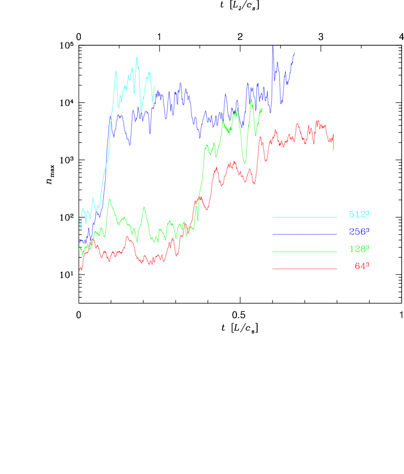
Figure 6: Evolution of the maximum density $n_{\rm max}$ in four simulations with the same global parameters (turbulent Mach number $\sim 10$, Jeans number $J=4$) at resolutions $64^{3}$ (red line), $128^{3}$ (green line), $256^{3}$ (dark-blue line), and $512^{3}$ (light-blue line). The time axis is given in units of the sound crossing time (lower axis), equal to 20 Myr, and of the quantity $L_{\rm J}/c_{\rm s}$ (upper axis), which is close to the free-fall time. The density axis is in units of the mean density in simulations $n_{0}=500{\rm~{}cm}^{-3}$. The first collapse event in each run is denoted by the sharp transition from a low mean maximum density level to a high one. The “collapse time” of the simulation is defined as the duration of the sharp rise of $n_{\rm max}$ over more than one order of magnitude separating the two levels. This is well defined in all cases except at $64^{3}$.

The limited resolution might also possibly affect the collapse times measured in the simulation (see §3.2.1), both because of the saturation values of the density reached by the collapsed objects as well as because of the possible slowing down of the collapse due to numerical viscosity. To test for this, Figures 6 and 7 illustrate the dependence of collapse on resolution. Figure 6 shows the evolution of the maximum density $n_{\rm max}$ in four simulations with the same global parameters (turbulent Mach number $\sim 10$, Jeans number $J=4$) at resolutions $64^{3}$ (red line), $128^{3}$ (green line), $256^{3}$ (dark-blue line), and $512^{3}$ (clear-blue line). The collapse in each simulation consists of the sharp transition from a low typical level of the maximum density ($n_{\rm max}\lesssim 100~{}n_{0}=5\times 10^{4}{\rm~{}cm}^{-3}$) to a high one ($n_{\rm max}\gtrsim 10^{3}~{}n_{0}=5\times 10^{5}{\rm~{}cm}^{-3}$). We define the “collapse time” of the simulations as the duration of the sharp rise of $n_{\rm max}$ over more than one order of magnitude separating the two levels. This is well defined for resolutions equal or larger than $128^{3}$. For economy reasons, the simulation at $512^{3}$ (i.e., R3) is only run for a short time compared to the other simulations. In all cases, there is seen to be a rebound from the maximum.

Figure 7 summarizes the collapse times as a function of resolution. For the $128^{3}$ simulation the collapse time corresponds directly to the measured duration of the rise of $n_{\rm max}$ for the first collapse, and the error bar denotes the full width of the rebound around the saturated value. For the $256^{3}$ (R1) and $512^{3}$ (R3) simulations, the collapse times correspond to the average of the durations measured for the available collapse events. The error bars denote the range of values found. This figure shows that the collapse time appears to be independent of resolution for resolutions $128^{3}$ and above, meaning that our longer-than-free-fall collapse times are not an artifact of the resolution. If anything, Figure 7 shows that there is a slight trend of the collapse time to increase with resolution, probably suggesting that the effect of traversing a larger dynamic range in density at higher resolution dominates over any slowing down of the collapse by numerical viscosity at lower resolution.

2. The simulations do not include ambipolar diffusion (AD). Even though the simulations were supercritical, in the presence of AD there would exist the possibility that some failed cores could be “captured” by AD if the main agent supporting them is the magnetic energy, since in this case AD could cause a redistribution of the magnetic field, leaving the centermost parts of the core with less support than in the case without AD. This, however, does not appear to be the case. For example, the longest-lasting failed core in R1, with a lifetime of $\sim 1.9$ Myr defined at $n_{\rm thr}=3\times 10^{4}{\rm~{}cm}^{-3}$, is clearly supercritical ($\mu\approx 4.0\pm 2.1$ times critical, where the uncertainty comes from the estimation of its “radius”, since the core is far from spherical; see Paper I), indicating that its failure to collapse was due to thermal+turbulent rather than magnetic support.

In any case, a worst-case estimate of the error committed by the lack of AD can be made by assuming that all failed cores with lifetimes longer than a representative AD timescale $\tau_{\rm AD}$ proceed to collapse rather than rebound. A reasonable estimate for $\tau_{\rm AD}$ is $\sim 1.5$ Myr (see the Appendix in Paper I). Being even more restrictive, we recalculated the number ratios assuming that the failed cores in R1 with lifetimes $\tau>0.9$ Myr are “captured” by AD (see Fig. 8). In this case, we find that the estimated number ratios of failed cores decrease by a factor of $\sim 2$, but this does not significantly affect the starless to stellar core ratio, because the failed cores have very low masses.

4.3 Conclusions

In spite of its limitations, the results of the present study are nevertheless encouraging, as the prestellar lifetimes measured directly from the density evolution of the cores are in good agreement with observational determinations. The same is true for the number ratios of prestellar to stellar cores. This estimation depends on the free parameter $\tau_{\rm yso}$, but a single value for it, chosen as the mean of the range reported by Hatchell et al. (2007) for Perseus, produces number ratios that are in good agreement with observational determinations at both high and low values of the density threshold $n_{\rm thr}$. The present study thus suggests that the turbulent model of star formation is not inconsistent with observational determinations of core lifetimes and the number ratios of prestellar to stellar cores.

Figure 2: Peak density as function of time for collapsing cores in R1 (upper panel), R2 (middle panel) and R3 (lower panel) after they have exceeded $n_{\mathrm{pk}}=6\times 10^{4}{\rm~{}cm}^{-3}$. A merging event occurs among the first two collapsing cores of R1 (solid and dashed lines respectively), but their peak densities are seen to rise steeply before their merger (the time when the lines converge). A merger also occurs in R2, but well after the individual collapse of the cores.

Figure 3: Duration of the prestellar stage for the collapsing cores in the simulations as a function of their mean density at the time collapse starts being measured. Diamonds, triangles and squares respectively correspond to the R1, R2 and R3 runs. The loci of $\tau_{\mathrm{pre}}=\tau_{\rm ff}$ and $\tau_{\mathrm{pre}}=10~{}\tau_{\rm ff}$ is marked by the lower and upper long-dashed lines respectively. Also shown is the fit for the mean prestellar lifetime as a function of mean density (dash-dotted line), which is $\simeq 6~{}\tau_{\rm ff}$.

Figure 5: Left: Size histogram of the failed cores at $n_{\rm thr}=30~{}n_{0}=1.5\times 10^{4}{\rm~{}cm}^{-3}$ for R1. Right: Mass histogram for the same cores.

Figure 7: Collapse time versus resolution for the three highest-resolution runs shown in Fig. 6. For the $128^{3}$ simulation, this time corresponds to the measured duration of the rise of $n_{\rm max}$ for the first collapse, and the error bar denotes the full width of the rebound around the saturated value. For the $256^{3}$ and $512^{3}$ simulations, collapse times correspond to the average of the durations measured for the collapse events shown in Fig. 2. The error bars denote the range of values found.

Figure 8: Same as Fig. 4 but assuming that all failed cores with lifetimes $\tau>0.9$ Myr are “captured” by AD and led to gravitational collapse. The fraction of failed cores is seen to decrease, but their masses are so small that the fraction of stellar cores remain essentially unchanged.

References

- Ballesteros-Paredes et al. (1999a) Ballesteros-Paredes, J., Vázquez-Semadeni, E., & Scalo, J. 1999a, ApJ, 515, 286
- Ballesteros-Paredes et al. (1999b) Ballesteros-Paredes, J., Hartmann, L., & Vázquez-Semadeni, E. 1999b, ApJ, 527, 285
- Ballesteros-Paredes et al. (2006) Ballesteros-Paredes, J., Gazol, A., Kim, J., Klessen, R. S., Jappsen, A.-K., & Tejero, E. 2006, ApJ, 637, 384
- Ballesteros-Paredes & Hartmann (2007) Ballesteros-Paredes, J., & Hartmann, L. 2007, Rev. Mex. AA, 43, 123
- Ballesteros-Paredes et al. (2007) Ballesteros-Paredes, J., Klessen, R., Mac Low, M.-M., & Vázquez-Semadeni, E. 2007, in Protostars and Planets V, ed. B. Reipurth, D. Jewitt, & K. Keil (Tucson: Univ. of Arizona Press), 63
- Beichman et al. (1986) Beichman, C. A., Myers, P. C., Emerson, J. P., Harris, S., Mathieu, R., Benson, P. J., & Jennings, R. E. 1986, ApJ, 307, 337
- Blitz (1993) Blitz, L., 1993, in Protostars and Planets III, ed. E. H. Levy, & J. I. Lunine (Tucson: Univ. of Arizona Press), 125
- Ciolek & Basu (2001) Ciolek, G. E., & Basu, S. 2001, ApJ, 547, 272
- Crutcher (1999) Crutcher, R. M. 1999 ApJ, 520, 706
- Elmegreen (1993) Elmegreen, B. G. 1993, ApJ 419, L29
- Elmegreen (2000) Elmegreen, B. G. 2000, ApJ, 530, 277
- Fatuzzo & Adams (2002) Fatuzzo, M., & Adams, F. C. 2002, ApJ, 570, 210
- Fiedler & Mouschovias (1993) Fiedler, R. A., & Mouschovias, T. 1993 ApJ, 415, 680
- Gómez et al. (2007) Gómez, G. C., Vázquez-Semadeni, E., Shadmehri, M., & Ballesteros-Paredes, J. 2007, preprint (arXiv:0705.0559)
- Greene et al. (1994) Greene, T. P., Wilking, B. A., Andre, P., Young, E. T., & Lada, C. J. 1994, ApJ, 434, 614
- Hartmann et al. (2001) Hartmann, L., Ballesteros-Paredes, J., & Bergin, E. A. 2001, ApJ, 562, 852
- Hatchell et al. (2007) Hatchell, J., Fuller, G. A., Richer, J. S., Harries, T. J., & Ladd, E. F. 2007, A&A, 468, 1009
- Heitsch et al. (2004) Heitsch, F., Zweibel, E. G., Slyz, A. D., & Devriendt, J. E. G. 2004, ApJ, 603, 165
- Heyer & Brunt (2004) Heyer, M. H., & Brunt, C. M. 2004, ApJ, 615, L45
- Heyer & Brunt (2007) Heyer, M. H., & Brunt, C. M. 2007, in IAU Symposium 237, Triggered Star Formation in a Turbulent ISM, ed. B. Elmegreen & J. Palous (Cambridge: Cambridge University Press), 9
- Jijina et al. (1999) Jijina, J., Myers, P. C., & Adams, F. C. 1999, ApJS, 125, 161
- Jrgensen et al. (2007) Jørgensen, J. K., Johnstone, D., Kirk, H., & Myers, P. C. 2007, ApJ, 656, 293
- Kenyon et al. (1990) Kenyon, S. J., Hartmann, L. W., Strom, K. M., & Strom, S. E. 1990, AJ, 99, 869
- Kenyon & Hartmann (1995) Kenyon, S. J., & Hartmann, L. 1995, ApJS, 101, 117
- Kim et al. (1999) Kim, J., Ryu, D., Jones, T. W., & Hong, S. S. 1999, ApJ, 514, 506
- Kirk et al. (2006) Kirk, H., Johnstone, D., & Di Francesco, J. 2006, ApJ, 646, 1009
- Kirk et al. (2005) Kirk, J. M., Ward-Thompson, D., & André, P. 2005, MNRAS, 360, 1506
- Larson (1969) Larson, R. B. 1969, MNRAS, 145, 271
- Larson (1981) Larson, R. B. 1981, MNRAS, 194, 809
- Lee & Myers (1999) Lee, C. W., & Myers, P. C. 1999, ApJS, 123, 233
- Mac Low & Klessen (2004) Mac Low, M.-M., & Klessen, R. S. 2004, Rev. Mod. Phys., 76, 125
- Maddalena & Thaddeus (1985) Maddalena, R. J., & Thaddeus, P. 1985, ApJ, 294, 231
- Mouschovias (1976) Mouschovias, T. C. 1976, ApJ, 207, 141
- Mouschovias (1991) Mouschovias, T. Ch. 1991, in The Physics of Star Formation and Early Stellar Evolution, ed. C. J. Lada, & N. D. Kylafis (Dordrecht: Kluwer), 449
- Nakamura & Li (2005) Nakamura, F., & Li, Z.-Y. 2005, ApJ, 631, 411
- Onishi et al. (2002) Onishi, T., Mizuno, A., Kawamura, A., Tachihara, K., & Fukui, Y. 2002, ApJ, 575, 950
- Padoan & Nordlund (2002) Padoan, P., & Nordlund, Å 2002, ApJ, 576, 870
- Shu et al. (1987) Shu, F. H., Adams, F. C., & Lizano, S. 1987, ARA&A, 25, 23
- Stone et al. (1998) Stone, J. M., Ostriker, E. C., & Gammie, C. F. 1998, ApJ, 508, L99
- Taylor et al. (1996) Taylor, S. D., Morata, O., & Williams, D. A. 1996, A&A, 313, 269
- Truelove et al. (1997) Truelove, J. K., Klein, R. I., McKee, C. F., Hilliman, J. H. II., Howell, L. H., & Greenough, J. A. 1997, ApJ, 489, L179
- Vázquez-Semadeni et al. (1997) Vázquez-Semadeni, E., Ballesteros-Paredes, J., & Rodríguez, L. F. 1997, ApJ, 474, 292
- Vázquez-Semadeni et al. (2000) Vázquez-Semadeni, E., Ostriker, E. C., Passot, T., Gammie, C., & Stone, J. 2000, in Protostars and Planets IV, ed. V. Mannings, A. Boss, & S. Russell (Tucson: Univ. of Arizona Press), 3
- Vázquez-Semadeni et al. (2005a) Vázquez-Semadeni, E., Kim, J., Shadmehri, M., & Ballesteros-Paredes, J. 2005a, ApJ, 618, 344 (Paper I)
- Vázquez-Semadeni et al. (2005b) Vázquez-Semadeni, E., Kim, J., & Ballesteros-Paredes, J. 2005, ApJ, 630, L49
- Vázquez-Semadeni (2007) Vázquez-Semadeni 2007, in IAU Symp. 237, Triggered Star Formation in a Turbulent ISM, ed. B.G. Elmegreen, & J. Palous (Dordrecht: Kluwer), 50
- Ward-Thompson et al. (2007) Ward-Thompson, D., Andre, P., Crutcher, R., Johnstone, D., Onishi, T., & Wilson, C. 2007, in Protostars and Planets V, ed. B. Reipurth, D. Jewitt, & K. Keil (Tucson: Univ. of Arizona Press), 33
- Wilking et al. (1989) Wilking, B. A., Lada, C. J., & Young, E. T. 1989, ApJ, 340, 823
- Williams et al. (1994) Williams, J. P., de Geus, E. J., & Blitz, L. 1994, ApJ, 428, 693