Simulating spin systems on IANUS, an FPGA-based computer

Abstract

We describe the hardwired implementation of algorithms for Monte Carlo simulations of a large class of spin models. We have implemented these algorithms as VHDL codes and we have mapped them onto a dedicated processor based on a large FPGA device. The measured performance on one such processor is comparable to $O(100)$ carefully programmed high-end PCs: it turns out to be even better for some selected spin models. We describe here codes that we are currently executing on the IANUS massively parallel FPGA-based system.

, , , , , , , , , , , , , , , , ,

1 Introduction

Numerical simulations with Monte Carlo (MC) techniques of spin systems that show a complex behavior (as, for example, because of the presence of frustrated quenched disorder, the so called spin glasses) require huge computational efforts: the non-trivial structure of the energy-landscape, the long decorrelation time of the dynamics, the need to analyze several different realizations of the system all conspire to make the problem very challenging to clarify numerically. Reference [1] gives an introduction to numerical spin glass systems, and discusses and elucidates a number of relevant details.

One of the bottom lines is that traditional computers are not optimized towards the computational tasks that are relevant in a context of discrete variables: a large part of the needed CPU time is spent essentially performing logical operations on individual bits or on variables that can only appear in a few states, at variance with arithmetics on long data words (32 or 64 bits) which is the typical workload for which computers are optimized today. This problem can be turned into an opportunity by the proposal to develop a dedicated computer optimized to handle the typical workload associated to these applications. The use of Field Programmable Gate Arrays (FPGAs) adds flexibility to a dedicated architecture: an FPGA based system can be configured on-demand to perform with potentially very high efficiency on a variety of different algorithms.

The FPGA approach for the simulation of spin systems has been proposed several years ago [2], and is now revisited in the IANUS project, a massively parallel modular system based on a building block of 16 high-performance FPGAs. The IANUS architectural concept has been described in [3], while details of the hardware prototype, currently undergoing final tests, will be described elsewhere [4]. In this paper we focus on algorithm mapping: we explore several avenues to map Monte Carlo algorithms for spin systems on FPGAs, provide benchmark results for the performance of several associated implementations, and present some very preliminary results of large scale numerical simulations, quantifying the potential performance of full-scale IANUS systems.

This paper is structured as follows: Section 2 describes the spin models and the algorithms we have implemented as our first application for IANUS. Section 3 gives details about the FPGA-based implementation of those models and algorithms, covering various aspects of the VHDL design. In section 4 we present some results and performance figures for the test simulations of two different spin models. Section 5 draws the conclusions of the work developed so far, and outlines prospects for the near future.

2 Monte Carlo simulations of Spin Glass systems

2.1 Models

IANUS has been designed as a multipurpose reprogrammable computer; its first application is the simulation of spin models. We are interested in discrete models whose variables (the spins) sit at the vertexes of a $D-$dimensional lattice (the sites of the system). The spin variable associated to site $i$ ($s_{i}$) take only a discrete and finite set of values (in some cases, just two values).

We define an energy or cost function (the Hamiltonian $H$) that drives the dynamics of the system. Configurations of the system that appear in the course of the dynamics, once reached an equilibrium state, are distributed according to the probability function

$$P\sim e^{-\beta H}\;,$$ (1)

where $\beta$ is the inverse of the temperature $T$ and tunes the features of the type of configurations that appear at equilibrium: when $\beta$ becomes large only configurations that minimize $H$ are important (when $\beta\to\infty$ one looks for optimal configurations, i.e. minima of $H$), while when $\beta\to 0$ the weight is not important and spin configurations become equiprobable. Our local dynamics will allow us, in this way, to determine important features of physical systems or for example, in very strict analogy with it, of sets of equalities we want to satisfy.

Each spin only interacts with its nearest neighbors, i.e. with spins sitting at sites that are exactly one lattice spacing far away. The strength of the interaction of spins $s_{i}$ and $s_{j}$ is proportional to the value of a coupling $J_{ij}$, which in some models (the classical Ising model) is constant over all the bonds of the lattice (i.e. the connections among two first neighboring sites), or can vary randomly from pair to pair (in this case, for a given realization of the model, $J_{ij}$ depends on $i$ and $j$: it is fixed when defining the realization of the model and does not change during the dynamics). The model can be extended by adding an external magnetic field $h_{i}$ at every site ($h_{i}$ can also be a random variable), or also by considering the case of a diluted lattice (only certain sites of the lattice are occupied by spins, while the others are empty, depending on the value of the dilution, $x_{i}=0,1$).

A generic Hamiltonian for two-state ($s_{i}=\pm 1$) models has the form

$$H-\sum_{<i,j>}J_{ij}x_{i}x_{j}s_{i}s_{j}-\sum_{i}h_{i}x_{i}s_{i}\;,$$ (2)

where $<i,j>$ means that the sum is taken on all pairs of neighboring sites of the lattice.

Hamiltonians of the form (2) define several very interesting models. For instance, the Edward-Anderson (EA) spin glass [5] has $x_{i}=1$ and $h_{i}=0$ for all sites $i$, while $J_{ij}$ takes random values ($\pm 1$ in our work) with both positive and negative support. The random field Ising model (RFIM) [6, 7] has $x_{i}=1$ and $J_{ij}=1$ everywhere, but the field at each site takes random values $h_{i}=\pm\left|h\right|$. Another interesting case is the diluted antiferromagnet in a field (DAFF) [8], that has $J_{ij}=-1$ and $h_{i}=h$ everywhere while dilution $x_{i}$ takes randomly the value 0 or 1.

Models with two-state variables associated to the Hamiltonian (2) are usually referred to as Ising-like and their implementation on our FPGA-based computer are extensively discussed in this paper. Many other different spin models are very important: they have for example higher space dimensionality or are defined on non regular random graphs, longer range interactions or multivalued spin variables (for example the Potts models). In this note we also discuss the implementation of the dynamics of a four-state glassy Potts model [9], defined by the Hamiltonian

$$H=-\sum_{<i,j>}\delta_{s_{i}\pi_{i,j}({\mathrm{s}}_{j})}\;,$$ (3)

where the sum runs over first-neighbor sites, and the site variables $s_{i}$ can take four values. $\pi_{i,j}$ are quenched random permutations of $(0,1,2,3)$ (there are $4!$ of them): the pair of first neighboring spins $(s_{i},s_{j})$ has non zero energy only if $s_{i}=\pi_{i,j}(s_{j})$. This model displays a number of features that are typical of structural glasses, and could hopefully help describe the glassy state, that stays difficult to understand.

2.2 Algorithms

Our goal is to analyze, by numerical Monte Carlo simulations, the properties of the models described above. We have implemented for the IANUS processor two well-known algorithms, namely Metropolis and Heat Bath.

Both algorithms update a single spin at a time: they sweep the entire lattice and then start again. After a (long enough) number of steps one reaches, as discussed before, an equilibrium state, and the spin configurations that appear during the dynamics are typical of the probability distribution (1).

In the case of the Metropolis algorithm we propose to update a spin $s_{i}$, and we calculate the corresponding energy change $\Delta E$. If $\Delta E<0$, the update makes the energy function lower, and change is accepted. Otherwise we do not necessarily refuse the update (this would be a $\beta=\infty$ dynamics, where we move to the closest local minimum of $H$) but we accept it with a probability $p_{M}=\exp(-\beta\Delta E)$.

In the case of the Heat Bath algorithm we directly select the new value of the spin with a probability proportional to the Boltzmann factor

$$P_{HB}(s_{i}=+1)=\frac{e^{-\beta E_{+}}}{e^{-\beta E_{+}}+e^{-\beta E_{-}}}\;,$$ (4)

where $E_{+}$ and $E_{-}$ are the local energies of the two spin configurations for spin $s_{i}$ pointing up ($s_{i}=+1$) or down ($s_{i}=-1$), respectively. Since when we change $s_{i}$ only a few terms of the energy function change (the ones containing spin $s_{i}$ and its first neighbors), this is a fast and easy computation.

We define one full MC sweep to be the iteration of these simple steps for all sites of the lattice. The spin configurations that appear during the dynamical process we are simulating are correlated: a spin configuration depends on the ones that appeared at former times, and only when we consider large time separation among two such configuration we can consider them as independent. In this way we can define a correlation time (that depends on $\beta$ and characterizes the dynamics), that we can roughly define as the number of Monte Carlo sweeps it takes to make two spin configurations uncorrelated (see refs. [10] and [11]). An estimate of this correlation time is usually calculated during the simulation, taking configurations at various times and measuring their correlation.

Other algorithms are used in some simulations, as they offer higher efficiency in decorrelating the spin configurations (see [12] for a review). On one side no very effective specialized algorithm exist, for example, for the very interesting case of spin glasses (we have in mind here mainly cluster algorithms), and their implementation on IANUS would probably not be very effective: so we do not use this kind of algorithms, and stay with simple, local dynamics. On the other side, algorithms like Parallel Tempering [13] are crucial for simulating complex systems like spin glasses, but their implementation on our FPGA based devices is a trivial add-on so we do not discuss them here.

3 Hardware implementation

3.1 Parallelism

The guiding line of our implementation strategy is to try to express all the parallelization opportunities allowed by the FPGA architecture, matching as much as possible the potential for parallelism offered by spin systems. Let us start by noticing that, because of the locality of the spatial interaction [12], the lattice can be split in two halves in a checkerboard scheme (we are dealing with a so-called bipartite lattice), allowing in principle the parallel update of all white (or black) sites at once. Additionally, one can further boost performance by updating in parallel more copies of the system. We do so by updating at the same time two spin lattices (see later for further comments on this point). Standard PCs cannot efficiently exploit all available parallelism for several reasons, the most fundamental one being memory architecture, that prevents the processor from gathering fast enough all variables associated to the computation. Sharing the simulation between several computers is an interesting parallel solution, but optimization has a bottleneck in the limited bandwidth and large latency associated to communication patterns (see [3]).

The hardware structure of FPGAs allows exploitation of the full parallelism available in the algorithm, with the only limit of logic resources. As we explain below, the FPGAs that we use (Virtex4/LX160 and Virtex4/LX200, manufactured by Xilinx) have enough resources for the simultaneous update of half the sites for lattices of up to $8^{3}$ sites. For larger systems there are not enough logic resources to generate all the random numbers needed by the algorithm (one number per update, see below for details), so we need more than one clock cycle to update the whole lattice. In other words, we are in the very rewarding situation in which: i) the algorithm offers a large degree of allowed parallelism, ii) the processor architecture does not introduce any bottleneck to the actual exploitation of the available parallelism, iii) performance of the actual implementation is only limited by the hardware resources contained in the FPGAs.

We have developed a parallel update scheme, supporting 3-D lattices with $L\geq 16$, associated to the Hamiltonian of (2). One only has to tune a few parameters to adjust the lattice size and the physical parameters defined in $H$. We regard this as an important first step in the direction of creating flexible enough libraries of application codes for an FPGA-based computers.

The number of allowed parallel updates depends on the number of logic cells availables in the FPGAs. For the Ising-like codes developed so far, we update up to $1024$ sites per clock cycle on a Xilinx Virtex4-LX200, and up to $512$ sites/cycle for the Xilinx Virtex4-LX160. The algorithm for the Potts model requires more logic resources and larger memories, so performances lowers to $256$ updates/cycle on both the LX200 and LX160 FPGAs.

3.2 Algorithm Implementation

We now come to the description of the actual algorithmic architecture, shown in fig. 1.

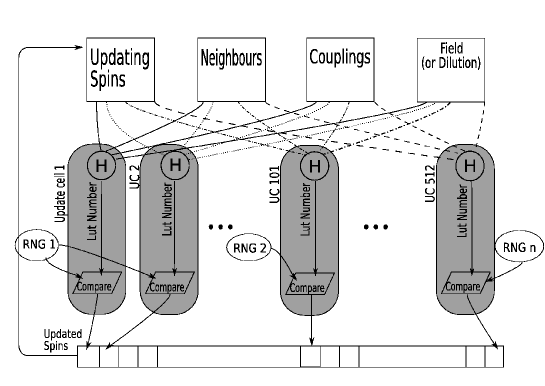
Figure 1: Parallel update scheme. The spins that must be updated, their neighbors, the couplings and all other relevant values are passed to the update cells where the energy is computed. The result is used as a pointer to a Look-up Table (LUT). The associated value is compared with a random number (RNG), and following the comparison, the updated spin value is computed.

In short, we have a set of update cells ($512$ in the picture): they receive in input all the variables and the parameters needed to perform all required arithmetic and logic operations, and compute the updated value of the spin variable. Data (variables and parameters) are kept in memories and are fed to the appropriate update cell. Updated values are written back to memory, to be used for subsequent updates.

The choice of an appropriate storage structure for data and the provision of enough data channels to feed all update cells with the data they need is a complex challenge; designing the update cells is a comparatively minor task. Hence we describe first the memory structures of our codes, followed by some details on the architecture of the update cells.

Virtex-4 FPGAs have several small RAM-blocks that can be grouped together to form bigger memories. We use these blocks to store all data items: spins, couplings, dilutions and external fields. The configurable logic blocks are used for random number generators and update cells.

To update one spin of a three dimensional model we need to read its six nearest neighbors, six couplings, the old spin value (for the Metropolis algorithm) and some model-dependent information such as the magnetic field for RFIM and the dilution for DAFF. All these data items must be moved to the appropriate update cells, in spite of the hardware bottleneck that only two memory locations in each block can be read/written at each clock cycle.

Let us analyze first the Ising models, considering for definiteness $L=16$. We choose to use an independent memory of size $L^{3}$ for each variable. This is actually divided into smaller memories, arranged so that reading one word from each gives us all the data needed for a single update cycle. We need $16^{3}=4096$ bits to store all the spins of one replica. We have $16$ vertical planes, and save each plane in a different memory of width $16$ bits and height $16$ (see Fig.2). In this simple case the logic resources within the FPGA allow to update one whole horizontal plane in one clock cycle (because we mix the two bipartite sublattices of two different copies of the system, see the following discussion), and the reading rate matches requirements, as we need to read only one word from each of the sixteen memories.

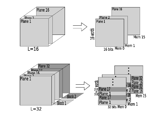
Figure 2: Examples of the spin memory structure: L=16 and L=32.

The configuration is slightly more complex when the size of the lattice grows and the update of a full plane in just one clock cycle is no longer possible. In this case we split each plane in a variable number of blocks $N_{B}$, adjusted so that all the spins of each block can be updated in one clock cycle. The number of independent memories is $L/N_{B}$, as only these need to be read at the same time. The data word still have width $L$, while the height is $L\times N_{B}$ to compensate for the reduced number of memories. Considering $L=32$, for example, we have a plane made of $32^{2}=1024$ spins, too large to be updated in one cycle (in the Xilinx Virtex4-LX160). We split it in two blocks of $32\times 16=512$ spins each. To read $16$ lines every clock cycle we store the spins into $16$ memories, each of width $32$ bits and height $32\times 2$: the total size of the memory is still $32^{3}$ bits.

As already remarked, we simulate two different replicas in the same FPGA. This trick bypasses the parallelism limit of our MC algorithms (nearest neighbors cannot be updated at the same time, see [3] ). We mesh the spins of the two replicas in a way that puts all the whites of one replica and the blacks of the other in distinct memories that we call respectively $P$ and $Q$ (see Fig.3). Every time we update one slice of $P$ we handle one slice of whites for replica $1$ and one slice of blacks for replica $2$. Obviously the corresponding slice of memory $Q$ contains all the black neighbors of replica $1$ and all the white neighbors of replica $2$.

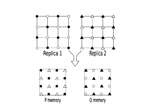
Figure 3: Structure of spin configuration memories: meshing of replicas.

The amount of memory available in the FPGA limits the lattice size we can simulate and the models we can implement. In both the Virtex4-LX160 and LX200 it is possible to simulate EA, RFIM and DAFF models in $3D$ with size up to $L=88$ (not all smaller sizes are allowed). Because of the dramatic critical slowing down of the dynamics of interesting complex spin models these size limits are confortably larger of what we can expect to be able study (even with the tremendous power made available by IANUS) in a reasonable amount of (wall-clock) time: memory size is presently not a bottle-neck.

Things are even more complicated when one considers multi-state variables, as more bits are required to store the state of the system and all associated parameters. In the four state Potts model (see sec. 2.1) the site variables need two bits and the couplings eight bits. In order to keep a memory structure similar to that outlined before we store each bit in a different memory. For example a lattice with $L=16$ requires $16\times 2$ memories for the site variables (they were sixteen in the Ising case), and $16\times 8$ memories for the couplings.

The lattice meshing scheme is maintained. With our reference FPGAs we can simulate three dimensional Potts model with at most $L=40$ and four dimensional Potts model with $L=16$.

We now come to the description of the update cells. The Hamiltonian we have written is homogeneous: the interaction has the same form for every site of the lattice, and it only depends on the values of the couplings, the fields and the dilutions. This means that we can write a standard update cell and use it as a black box to update all sites: it will give us the updated value of the spin (provided that we feed the correct inputs). This choice makes it easy to write a parametric program, where we instantiate the same update cell as many times as needed.

We have implemented two algorithms: Metropolis and Heat Bath. The update cell receives in input couplings, nearest neighbors spins, field and dilution and, if appropriate, the old spin value (for the Metropolis dynamics). The cell uses these values as specified by (2) and computes a numerical value between $0$ and $15$ (the range varies depending on the model) used as an input to a LUT. The value read from the LUT is compared with a random number and the new spin state is chosen depending on the result of the comparison. Once again, things are slightly different for the Potts model due to the multi-state variables and couplings.

Our goal is to update in parallel as many variables as possible, which means that we want to maximize the number of cells that will be accessing the LUT at the same time. In order to avoid routing congestion at the hardware layer we replicate the LUTs: each instance is read only by two update cells. The waste in logic resources – the same information is replicated many times within the processor – is compensated by the higher allowed clock frequency.

3.3 Random numbers

Monte Carlo methods depend strongly on the random numbers used to drive the updates: this determines the imperative need to implement a very reliable pseudo-random number generator (RNG), that produces a sequence of numbers under the selected distribution, with no known or evident pathologies.

We use the Parisi-Rapuano shift register method [16] defined by the rules:

$$I(k) = I(k-24)+I(k-55)$$ (5)

$$R(k) = I(k)\otimes I(k-61)\;,$$

where $I(k-24)$, $I(k-55)$ and $I(k-61)$ are elements (32-bit wide) of a so called wheel that we initialize with externally generated random values. $I(k)$ is the new element of the updated wheel, and $R(k)$ is the generated pseudo-random value.

A straightforward implementation of this algorithm produces one random number at each step, for each wheel that we maintain. A wheel uses many hardware resources (in our case we use the three pointer values $24$, $55$ and $61$ so we need to store $62$ numbers), and the random number generator is a system bottleneck, since the number of updates per clock cycle is limited by how many random values we are able to produce. A large performance improvement comes from the implementation of the wheel through logic (as opposed to memory) blocks, as the former can be written in cascade-structured combinatorial logic that may be tuned to produce several numbers per clock cycle. We can exploit this feature and use a limited number of wheels to produce more numbers, thus increasing the number of updates per clock. Remember that to produce one random number we must save the result of the sum of two values and then perform the XOR with a third value. The wheel is then shifted and the computed sum fills the empty position. All this is done with combinatorial logic, so one can produce various pseudo-random numbers simply replicating these operations and, of course, increasing logic complexity. A schematic representation of a simplified case is given in fig. 4.

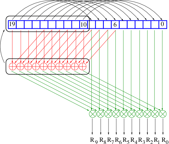
Figure 4: Hardware implementation of the Parisi-Rapuano RNG. For graphical reasons the example refers to a wheel of only 20 numbers and following the reduced equations $I(k)=I(k-10)+I(k-14)$ and $R(k)=I(k)\otimes I(k-20)$. The combinatorial logic complexity grows when producing more numbers.

The logic complexity of the implementation depends on the parameters of (5) and on the quantity of random numbers we need. We use one wheel to generate up to $96$ numbers per clock (so more wheels are active at the same time to compute all needed random values).

To keep the wheel safely below its period limit we choose to reload the wheel every now and then (for example every $10^{7}$ MC sweeps).

With respect to the choice of $32$-bit random numbers, we have verified that this word size is sufficient for the models we want to simulate (our tests show that $24$-bit would be enough). Other models may require better random numbers. We do not address this issue here. We just note that generating random numbers of larger size (e.g., $40$ or even $64$-bit) would be straightforward, at the price, of course, of a larger resource usage.

All in all, our carefully handcrafted VHDL codes use a very large fraction of the available FPGA resources, as measured by the number of used logic blocks and RAM-blocks. The following table shows figures for the Ising-like and Potts-model codes. Mapping has been performed with the ISE toolkit made available by Xilinx. The Ising-like code is limited by logical resources, while the Potts model, with its larger storage requirements, is limited by available memory space.

Model	Resource	Number used	% (LX160)	% (LX200)
Ising-like	Log. blocks	$157,649$	$(117\%)$	$88\%$
(1024 updates)	RAM-blocks	$160$	$56\%$	$47\%$
Ising-like	Log. blocks	$83,651$	$62\%$	$46\%$
(512 updates)	RAM-blocks	$80$	$28\%$	$23\%$
Potts $q=4$	Log. blocks	$117,586$	$86\%$	$66\%$
(256 updates)	Ram-blocks	$224$	$77\%$	$67\%$

Table 1: Use of FPGA resources, as absolute values and as fraction of available blocks on our FPGAs, for the Ising-like and Potts codes. In both cases, the 3-D lattice has a linear size $L=32$. The Ising-like code is limited by available logic resources , while the Potts code is memory-limited.

4 Benchmark tests

4.1 Edward-Anderson spin glass model

We have simulated an $L=32$ $3D$ system at $\beta(=1/T)=0.878$. The number of MC sweeps sums up to $8\times 10^{9}$. See reference [17] for previous simulations done with the special purpose machine SUE on a lattice of size $L=20$

Checking that thermalization has been reached is a common and non-trivial problem in spin glass simulations. Here we provide only a short review of our analysis: full details will be published elsewhere. In our early tests, configurations were copied to the host computer every $10^{6}$ MC sweeps, because, when performing these tests, we had a very slow communication channel to the host . This value is too high to see clearly the evolution towards equilibrium along the first sweeps. Fig. 5 shows the MC history of a physically meaningful quantity, the squared overlap $q^{2}$; a zoom of the leftmost part of the plot (inset graphic) shows the drift from the initial value ($0.045$) to a value probably very close to the equilibrium value in less then $50\times 10^{6}$ sweeps.

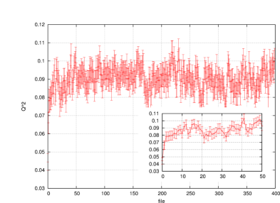
Figure 5: Evolution of $q^{2}$: the x-axis scale is $10^{6}$ MC sweeps per file

We have analyzed the thermalization rate also with the standard $log_{2}$L data binning: we divide the data points into four groups of variable size (namely the last half of the measures, then the previous quarter, the previous eighth and the sixteenth before this) and then average over all samples in each group. From the smaller $1/16$th to the bigger $1/2$ group the averaged value is expected to shift toward its equilibrium value. Fig. 6 shows the behavior of the squared overlap $q^{2}$. The time dependence we observe on the latest data is very small, it does not expose any systematic drift and is surely far smaller than the statistical error.

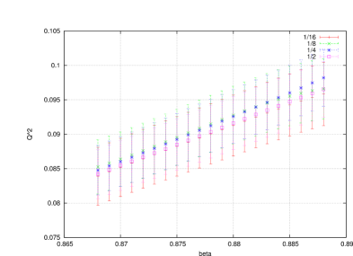
Figure 6: Thermalization test of the squared overlap $q^{2}$ as a function of $\beta=1/T$.

A clean visual representation of the system thermalization is also given via the average overlap probability distribution $P(q)$, which should be symmetric at equilibrium (with no external field), as shown in fig. 7: this is obviously only a necessary condition for thermalization, but it surely is a good sign.

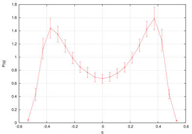
Figure 7: Distribution of the overlap $q$, showing a reasonably symmetric behavior, within error bars.

4.1.1 Performance

The algorithms described in the previous section are mapped on the selected FPGAs with a system clock of 62.5 MHz. At each clock cycle, $512$ ($1024$) spins are updated on an LX160 (LX200), corresponding to an average update time of $32$ ps/spin ($16$ ps/spin).

It is interesting to compare these figures with those appropriate for a PC. Understanding what exactly has to be compared is not completely trivial. The fastest PC code for spin model simulations available to us is the multi-spin coding, which updates in parallel a large number of (up to 128) samples of the system at the same time, using only one random number generator, which is shared across all samples: this scheme is useful to obtain a large number of configuration data, appropriate for statistical analysis. We call this an asynchronous multi-spin coding (AMSC) as inside each sample there is no parallelism.

As we have stated before, the biggest problem with the models we want to study is the decorrelation time, and the large number of Monte Carlo sweeps that it may take to bring a configuration to equilibrium. The AMSC procedure has a serious problem here since each sample evolves for the same number of sweeps as if it were the only one being simulated. In other words, efficient codes on a PC achieve high overall performance by simulating for relatively short MC time a large number of independent samples. A code that updates in parallel more spins belonging to the same system would be more useful to attain equilibrium, when working on large systems. The resulting algorithm, synchronous MSC (SMSC), takes less time to simulate one sample, but the global performance is lowered because of more complex operations involved and the need to use an independent random number for each spin. The SMSC PC-code available to us updates up to 128 spins of a single sample. Synchronous codes are not commonly used in PC based numerical simulations because of their globally poor performances.

Generally speaking we think that comparison with a SMSC code is appropriate for a single FPGA system, while comparison with an AMSC code is more relevant when considering a massively parallel IANUS system (we plan to build a system with 256 FPGA-based nodes). Here we simply present our preliminary comparison data for both cases in table 2.

	LX160	LX200	PC (SMSC)	PC (AMSC)
Update Rate	32 ps/spin	16 ps/spin	3000 ps/spin	700 ps/spin

Table 2: Comparing the performances of two Xilinx Virtex4 FPGAs and two different codes running on a high-end PC.

The MSC values are referred to an Intel Core2Duo (64 bit) 1.6 GHz processor. Inspection of table 2 tells us that one LX160 runs as fast as 90 PCs, while the LX200 performance is comparable to that of 180 PCs. In other words, the $8\times 10^{9}$ MC iterations required to thermalize a lattice of size $L=32$ took approximately $6$ hours to be completed on just one Virtex4-LX200: they would take $18$ days on a PC running the SMSC algorithm.

Performance comparison with published work is difficult. As far as we know the SMSC is not used for massive simulations, so data on the performances of this algorithm is not widespread. The AMSC is commonly used. Even if it is considered almost a standard in spin glass simulations, we have not been able to find recent speed analysis. The seminal works on this algorithm [14] and [15] are way too old in technology terms to allow a fair comparison. All in all, we believe that the codes that we have used for performance comparison are state-of-the-art PC implementations, and further optimizations could at most improve the performances by some $10-20\%$; we conclude that the performance of one FPGA-processor is roughly $\simeq 100$ times better than possible on a PC.

4.2 Potts model

Simulations for the three and four dimensional $L=16$ four-state Potts model have been run at various temperatures. Previous works on the $4D$ model [9] could only thermalize a lattice of size $L=5$, and study $L=8$ in the warm phase. To obtain good results with out tests we had to run long simulations, which took up to $18\times 10^{11}$ MC iterations for the $3D$ case ($\beta=2.4$) and $6\times 10^{10}$ in $4D$ ($\beta=1.405$).

Also in this case the thermalization has been analyzed using $log_{2}$ data binning. Fig. 8 shows the average $P(q)$ for the Potts disordered model. The symmetry is not as good as for the Ising spin glass.

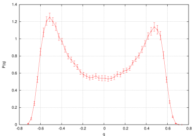
Figure 8: Distribution of the overlap $q$ for the four-states three dimensional Potts model with $L$ = 16 at $\beta=2.4$.

4.2.1 Performance

The update algorithm of the Potts model requires more complicated operations. We do not have an MSC version for this case but we do not expect great improvements compared with the non-MSC code we have used: the size of the spin variables (four bits) and the structure of the update algorithm do not leave as much space for parallelization and high performances on a PC as it was the case for the EA model. We expect that an optimized code would be at most twice faster (halving the times shown here).

Our FPGA-based implementation does not suffer the increased complexity as much as the PC generic architecture: apart from the smaller sizes permitted, the number of sites that can be updated at the same time reduces only by a factor four with respect to EA.

	LX160	LX200	PC
Potts 3D	125 ps/spin	64 ps/spin	117 ns/spin
Potts 4D	125 ps/spin	64 ps/spin	150 ns/spin

Table 3: Potts model performances in two Xilinx Virtex4 FPGAs and in a PC.

Table 3 shows the comparison with an Intel Pentium IV 3.2 GHz processor. Simulating a three dimensional lattice, the smaller LX160 performs as $900$ PCs approximately, while the LX200 works as fast as $1800$ PCs. In $4D$-models these numbers change respectively to 1200 for LX160 and 2300 for the LX200.

Once again we point out that these results refer to just one FPGA. A IANUS computer has $16$ FPGA devices per board, improving, with a (needed) embarrassing parallelism performance increased by a factor $16$: a complete IANUS computer will probably have $16$ boards, bringing this factor to $256$ and the performance global ratio of a LX200 based machine to a PC for a $4D$ disordered Potts model to a number of the order of half a million.

5 Conclusions

This paper has described the implementation on a FPGA based engine performing Monte Carlo simulation of some classes of spin models. The main results of our work can be summarized as follows:

• The simulation engine exploits all the parallelization space in principle available in the algorithm and its performance is limited only by available hardware resources.

• Measured performance are outstanding if compared with figures available for traditional PCs: one FPGA has the same performance as $\simeq 100$ PCs for the Edwards-Anderson spin glass model. Comparison data is even more impressive for the Potts model, whether the speed-up factor is close to $\simeq 1000$.

• The FPGA-based processor has shown stable operation for extended time periods: thanks to this reliable behavior we have been able to collect a large number of spin configurations.

The work described here will continue with actual physics runs in which large statistics will be collected for larger systems, as soon as large IANUS systems are available. We also continue to work on the development of simulation codes for other algorithms of scientific interest. Work is in progress in such areas as random graphs, surface growing and protein docking.

References

- [1] E. Marinari, G. Parisi and J. J. Ruiz-Lorenzo, Numerical simulations of spin glass systems, in Spin Glasses and Random Fields, (A. P. Young editor) World Scientific, Singapore, 1998.
- [2] A. Cruz, et al., Comput. Phys. Commun. 133 (2001) 165-176.
- [3] F.Belletti et al., Computing in Science and Engineering 8 (2006) 41-49.
- [4] the Ianus Collaboration, work in progress.
- [5] S. F. Edwards and P. W. Anderson, J. Phys. F: Mat. Phys. 5 (1975) 965-974.
- [6] Y. Imry and S. Ma, Phys. Rev. Lett. 35 (1975) 1399-1401.
- [7] D. P. Belanger and A. P. Young, J. of Magnetism and Magnetic Materials 100, (1991) pp. 272-291.
- [8] A. D. Ogielski and D. A. Huse, Phys. Rev. Lett. 56 (1986) 1298-1301.
- [9] E. Marinari et al., Phys. Rev. B, 59 (1999) 8401-8404.
- [10] A.D. Sokal, Monte Carlo Methods in Statistical Mechanics: Foundations and New Algorithms, Cours de Troisième Cycle de la Physique en Suisse Romande (1989)
- [11] D. J. Amit and V. Martín-Mayor, Field theory, renormalization group and critical phenomena (third edition) World Scientific, Singapore (2005)
- [12] D. P. Landau and K. Binder, A Guide to Monte Carlo Simulations in Statistical Physics Cambridge University Press (2005).
- [13] E. Marinari and G. Parisi, Europhys. Lett. 19 (1992) 451. K. Hukushima and K. Nemoto, J. Phys. Soc. Jpn. 65 (1996) 1604. M. C. Tesi et al. J. Stat. Phys. 82 (1996) 155.
- [14] H. O. Heuer, Comput. Phys. Commun. 59 (1990) 387-398.
- [15] H. Rieger, Jour. Stat. Phys, 70 (1993) 1063-1073.
- [16] G.Parisi and F. Rapuano, Phys. Lett. B 157 (1985) 301-302.
- [17] H.G. Ballesteros et al., Phys. Rev. B 62 (2000) 14237-14245.