Modeling diffusional transport in the interphase cell nucleus

Abstract

In this paper a lattice model for diffusional transport of particles in the interphase cell nucleus is proposed. Dense networks of chromatin fibers are created by three different methods: randomly distributed, non-interconnected obstacles, a random walk chain model, and a self avoiding random walk chain model with persistence length. By comparing a discrete and a continuous version of the random walk chain model, we demonstrate that lattice discretization does not alter particle diffusion. The influence of the 3D geometry of the fiber network on the particle diffusion is investigated in detail, while varying occupation volume, chain length, persistence length and walker size. It is shown that adjacency of the monomers, the excluded volume effect incorporated in the self avoiding random walk model, and, to a lesser extent, the persistence length, affect particle diffusion. It is demonstrated how the introduction of the effective chain occupancy, which is a convolution of the geometric chain volume with the walker size, eliminates the conformational effects of the network on the diffusion, i.e., when plotting the diffusion coefficient as a function of the effective chain volume, the data fall onto a master curve.

I Introduction

In recent years, great progress has been made in the view of the living cell as a regulatory network in time. On the other hand, the coupling of biochemical processes with the spatial arrangements of the cellular components is less understood. For a quantitative understanding of the function of the cell, one needs to link the existing one dimensional genomic, functional and metabolic information to its three dimensional organization. The main aspect is the quantitative description of the transport of biomolecules in the dense network of macromolecules that constitutes the major part of the cytoplasm and the cell nucleus.
Diffusive processes in the cell play a central role in keeping the organism alive organism1; organism2. Molecules transported through cell membranes, drugs on their way to their protein receptors and proteins interacting with specific DNA sequences constituting all of the biological functions of DNA alldiff1; alldiff2 are diffusion controlled reactions. Furthermore, proteins approaching their specific target sites on DNA are transported by diffusion or even facilitated diffusion Holger1; Holger2; fd1; fd2; fd3; fd4. For the 1D sliding motion experimental evidence exists exp1; exp2.
However, diffusional transport of molecules in the living cell is fundamentally different from the normal kind of diffusion which a molecule undergoes in a homogeneous fluid where the mean square displacement of a molecule behaves linear in time $t$, $\langle r^{2}(t)\rangle=6Dt$ with $D$ as the diffusion coefficient. The cellular environment is a crowded solution of macromolecules. In particular, the interphase cell nucleus constitutes a dense network of chromatin fibers with a volume fraction ranging from 5% to 12%. The motion of other macromolecules is strongly influenced by the presence of this ”sticky tangle” due to steric obstruction and transient binding. Fluorescence correlation spectroscopy (FCS) studies have shown obstructed diffusion of autofluorescent proteins wachsmuth; banks. Subdiffusion was also reported for other systems, for instance mRNA molecules and dense dextrans examp1; examp2. Obstructed diffusion or subdiffusion is characterized by $\langle r^{2}(t)\rangle\sim t^{\alpha}$ with the anomalous diffusion exponent $\alpha<1$. Subdiffusion like that might give rise to a weak ergocidity breaking, causing interesting effects in intracellular diffusion of macromolecules metzler.
Other FCS measurements indicate that most of the nuclear space is accessible to medium sized proteins by simple diffusion and that there is no preference for interchromosome territory channels weidemann. In general, macromolecular transport in the living cell nucleus is only rudimentarily understood. In particular, it is still a matter of intensive discussion wachsmuth to what extent macromolecular mobility is affected by structural components of the nucleus.
This paper shall contribute to the understanding of this process by developing a theoretical description of network diffusion in the interphase cell nucleus. There exist already theoretical descriptions of diffusion in the cell nucleus subdiffusion. However, these approaches do not incorporate realistic structures of the chromatin fibers. In the following the chromatin fibers are referred to as (polymer) chains and proteins diffusing through the fiber network are referred to as particles or walkers. In the present paper we investigate in detail how the diffusion coefficient of diffusionally transported particles of various size depends on the 3D geometry of the network of chromatin fibers and their density in the nucleus. Furthermore, we investigate to what extent structural properties of the fibers such as persistence length and contour length influence the diffusion coefficient.
The chromatin network in the cell nucleus during interphase is modeled using a lattice approach minimizing computational time and effort. The first method creates a crowded environment with polymer chains constructed by a random walk (RW) on the lattice without excluded volume. To confirm the accuracy of the lattice model, these results are also compared to simulations of the corresponding continuum model. Later, we introduce a self avoiding random walk (SAW) of well equilibrated polymer chains with excluded volume interaction, which deliver more realistic static properties such as end-to-end distance. These chains are simulated on the lattice by applying a simplified version of the bond fluctuation method BFM, the single site model, in combination with a Metropolis Monte Carlo (MC) procedure MC. The bond fluctuation model (BFM) was introduced as a new effective algorithm for the dynamics of polymers by Carmesin et al. BFM and provides a very effective means to simulate the dynamic behaviour of e.g. dense polymer melts Sommer1; Sommer2. Both methods, with RW and SAW chain model, are compared to a third test system consisting of disconnected, randomly distributed obstacles.
In section 2 the lattice for chain construction and particle diffusion is presented. A brief overview of the modeling of particles of different sizes is given, reflecting the diffusing proteins in the cell nucleus. In addition, the test system is described.
Section 3 introduces the RW chain model for the discrete and continuous space. We test the validity of the lattice approach by comparing the diffusion coefficient of particles in the discrete and the continuous model. Afterwards, the chain relaxation simulation is described. After presenting the results on particle diffusion in the RW chain model and the test system we conclude that the latter system is insufficient for a description of a chromatin fiber network. In section 4 the SAW chain model is introduced exhibiting important features of a real biological fiber network such as persistence length. The chain simulation algorithm is presented explaining shortly the BFM and MC procedure. It is shown that the static properties of the polymer chains in the SAW model agree with known scaling laws. Anomalous translational diffusion of the chains’ center of mass is observed. After stating the results on particle diffusion and comparing them to the RW chain model, it is concluded that the SAW chain model comes closer to the situation in the cell nucleus and thus yields more realistic diffusion coefficients. Finally, it is found that the diffusion coefficient of the particles depends on the persistence length of the fibers, but not on their contour length, as long as they consist of connected structures of several monomers. However, it does depend on the particular geometry composed by well equilibrated chains created by the SAW chain model. Section 5 summarizes the obtained results.

II Modeling volume

The model is contained in a $100\times 100\times 100$ cubic lattice. The penetrability of the lattice walls is different regarding chains and particle motion and is discussed in the following.

II.1 Particles

Proteins transported in the nucleus differ, among other things, in their size. For instance tracer particles with a size of 27 kD to 282 kD were used to study diffusional transport banks. In our model systems particles of different sizes are implemented by a corresponding numbers of occupied lattice sites in a cubic arrangement. We use three particle sizes: one occupied lattice site (small), a $2^{3}$ cube (medium) and a $3^{3}$ cube (large). In the continuous model spherical walkers of three different sizes are tested, the smallest walker being point-like with a radius $R_{walker}=0$, the medium sized particle with a radius $R_{walker}=1$ and the largest walker with a radius $R_{walker}=2$.

II.2 Diffusional transport simulation

The movement of a particle is modelled by a random walk. Particles are allowed to visit only unoccupied lattice sites. If a particle collides with a chain it is reflected to the last visited lattice site. The initial position is sampled randomly among non-occupied lattice sites. Then, random walks of different duration are carried out. To prevent boundary effects due to the lattice walls, periodic boundary conditions are applied.

II.3 Test system with disconnected obstacles

To study the influence of chain connectivity on particle diffusion, a test system is introduced with randomly distributed obstacles, occupying between 5% and 15% of the lattice sites.

III Random Walk Chain Systems

In this system the chromatin fibers are created by a standard random walk without excluded volume effects, i.e. allowing self intersection. This approach is more realistic than the set of disconnected obstacles of the test system, since here the monomers are interconnected to create fibers. This system is set up in both, lattice and continuum models, in order to justify the accuracy of the lattice approximation.

III.1 Model and chain simulation

In the discrete model the chromatin fibers are realized by chains of occupied connected lattice sites chosen by random walks on the $100\times 100\times 100$ lattice. In the continuous model the modeling volume is defined by a sphere of radius $R_{sphere}=50$ containing a chain of given length implemented by a random walk. To simulate a chain in the lattice model one site is chosen randomly as a starting point of the chain. During each random walk step one of the 6 nearest neighboring lattice sites is randomly selected with equal probability and is occupied. The walls of the modeling volume are reflecting, no flux boundary conditions are applied. The total number of occupied lattice sites yields the occupation volume. Simulations of random walks with lengths between 100000 and 700000 steps were carried out yielding occupation volumes between 6% and 36% (effective occupation volumes between 18% and 78%). The effective volume is defined in the next subsection.
In the continuous model a chain is created with a radius $R_{chain}=1$ using a random walk with step size of 5, which was chosen due to lower computational cost instead of a smaller step size. This is justified because of the self-similarity of the random walk which implies that the step size is irrelevant if the modeling volume is sufficiently large. The step size equals the segment length.
The volume exclusion effects are implemented in the following way: The chain is made of segments of radius $r$. The total geometric volume of the chain is computed via Monte Carlo integration (throw $10^{9}$ points into the system and count how many of them are inside the chain).

The walker is a sphere of radius $R$. Collision with the chain takes place if the distance to the chain is $<R+r$, but this is equivalent to a chain of thickness $R+r$ and point-like walker (because we use a simple random walk for the chain contour and do not consider chain-chain excluded volume). So the effective volume is again found via MC integration, but this time with chain radius $R+r$.

a

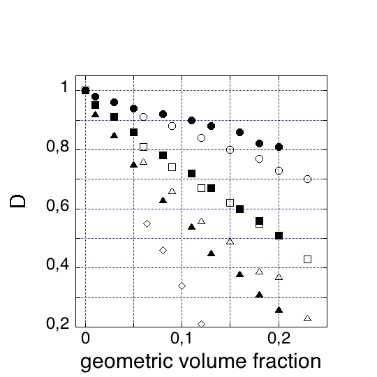
b

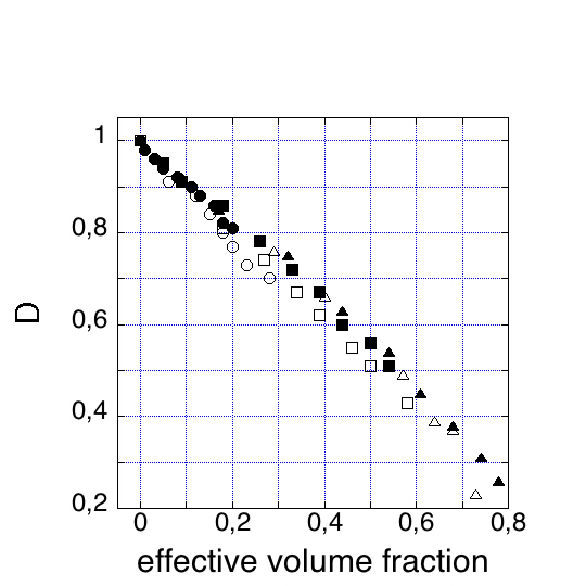
Figure 1: Comparison of the continuous and discrete random walk chain model and the test system (disconnected obstacles). Upper panel: Diffusion coefficient dependent on the geometric volume fraction. Lower panel: Diffusion coefficient dependent on the effective volume fraction. Circles: smallest particle, squares: medium sized particle, triangles: largest particle, and diamonds: medium sized particle in the test system. Blank: Discrete random walk chain model. Solid: Continuous random walk chain model.

III.2 Results

In the following the occupation volume of the lattice is either computed as the geometric volume or the effective volume. The geometric volume is defined as the total number of occupied lattice sites. The effective volume is defined as the space which is not freely accessible to a particle of given size. Hence, the effective volume of the chains on the lattice depends on the particle size. For a particle consisting of one occupied lattice site the geometric volume of the chain equals its effective volume.
One particle was randomly initialized in the lattice and in the spherical volume. 200000 random walk steps were carried out and the motion of the walker was monitored. This procedure was repeated 5000 times and the data were averaged. Fig. 1 shows the dependence of the diffusion coefficient on the geometric volume fraction and on the size of the particle in the lattice model and in the continuous model. In both models subdiffusion was observed around a geometric volume of 23% for the largest walker (Fig. 2), indicating it to be occasionally trapped. The anomalous diffusion exponent $\alpha=0.88$ was found by fitting the curve ”mean square displacement vs. $t$” with a power law. The non-adjacency of the occupied lattice sites in the test system was made responsible for a decreased diffusion coefficient compared to that of the random walk chain model: At a given value of the occupied geometric volume, the obstacles of the test system are more homogeneously distributed than the RW chains. This property is yielding a larger value for the effective occupation volume, so that walkers of large size are unable to find a percolation path around the obstacles. To the contrast, the random walk chains create regions of high density which are not accessible to the walker, but also leave areas of low density where a diffusion remains fairly unaffected.
Fig. 1 also shows the linear dependence of the diffusion coefficient on the effective volume fraction and on the size of the particle in the lattice model and in the continuous model respectively. The values lie on a straight line besides some slight deviations in the discrete model which may be due to the lattice discretization. This result reveals that in both models the effect of increasing either the size of the particle or the occupation volume of the chain is the same. Moreover,

$$D\propto\sigma_{free},$$ (1)

where $\sigma_{free}$ describes the volume fraction of the freely accessible space for a particle of given size.
The discrete and continuous model agree very well with another. The dependence of the diffusion coefficient on the occupation volume and the size of the walker is quantitatively the same in both models. Moreover, in both models subdiffusion is found in the same ranges of the geometric and effective occupation volume (Fig. 2).

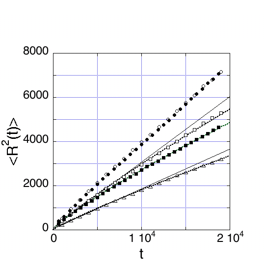
Figure 2: Mean square displacement of the largest particle vs. time. The continuous lines are linear fits through the first five points of the curve (blank squares, blank triangles) to illustrate the deviation from linearity for the long-time diffusion in the denser systems. The dashed lines are power law fits yielding the anomalous diffusion exponent $\alpha$. Blank circles: Random walk chain model (effective volume 68%, geometric volume 20%). Solid circles: Continuous random walk chain model (effective volume 68%, geometric volume 20%). Blank squares: Random walk chain model (effective volume 73%, geometric volume 23%, $\alpha=0.88$). Solid squares: Continuous random walk chain model (effective volume 78%, geometric volume 26%, $\alpha=0.85$). Triangles: Self avoiding random walk chain model (effective volume 81%, geometric volume: 12.5%, chain length $N=50$, $l_{p}=0.5$, $\alpha=0.89$).

III.3 Conclusions: RW chains

Due to the very good agreement of the results obtained with the discrete and the continuous model, we conclude that lattice discretization does not affect the characteristic properties of particle diffusion which are of interest in this work. Thus, for the rest of our investigations, the lattice model, being between one and two orders of magnitude faster than a corresponding continuum model, is employed. However, the adjacency of the chain monomers has an impact on particle diffusion. Hence, the test system, consisting of randomly distributed occupied lattice sites, is not a reasonable approximation to the properties of a crowded environment inside the cell nucleus.

IV Self Avoiding Random Walk Chain System

The SAW chain system incorporates two important characteristics of chromatin fibers in a biological system which are not considered in the RW chain model.
In the SAW chain system, chains are created by a self avoiding random walk, i.e. the excluded volume effect is taken into consideration. The chains are well equilibrated, relaxed and satisfy more realistic static properties such as end-to-end distance. Moreover, the chains exhibit a given persistence length reflecting a certain stiffness of the fiber.
Comparing the results on particle diffusion in this system to those of the RW chain system shows the dependence of the particle diffusion on the excluded volume effect and the persistence length.

a

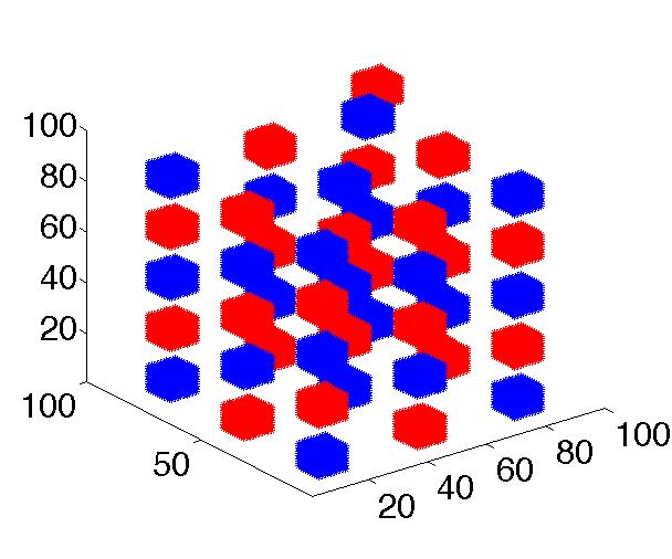
b

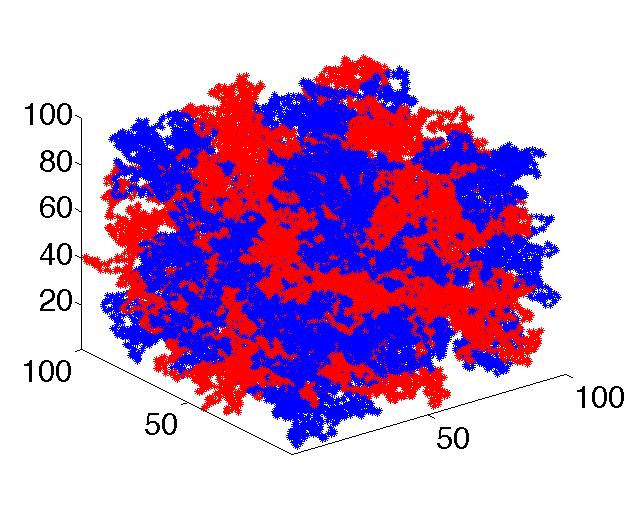
Figure 3: Upper panel: Start conformation of the Monte Carlo algorithm. 46 cubes, chains with $N=12^{3}$, are homogeneously distributed in the universe. Lower panel: Relaxed conformation after $6\cdot 10^{9}$ time steps of the Monte Carlo algorithm combined with the bond fluctuation method. The chains constitute a dense network, comparable with chromosome territories inside the cell nucleus. To highlight the topological structure of the chain network, the 46 chromosomes are alternately coloured, here red and blue.

IV.1 Model

The chromatin fibers are modelled by chains consisting of monomers connected by segments. Monomers are represented by occupied lattice sites. Neighboring occupied lattice sites reflect neighboring monomers in the chains. No lattice site is allowed to be occupied more than once. Possible bonds between two adjacent monomers are given by the set of all component permutations and sign inversions $P$ of two bond vectors:

$$P(1,0,0)\cup P(1,1,0).$$

The initial state for the Monte Carlo process consists of cubic compact chains. Cubes in the initial state have the dimension $L\times L\times L$ and are periodically distributed in the lattice (Fig. 3).
Every cube consists of $L$ planes of $L\times L$ occupied lattice sites. The occupied sites are connected in a way that a Hamiltonian path results. If $L$ is even, every plane of the cube is rotated by $90^{\circ}$ with respect to the previous one. Otherwise, if $L$ is odd, every second plane of the cube is rotated by $90^{\circ}$ with respect to the first one. The Hamiltonian path is afterwards reflected at the diagonal of the plane. Start and end point of the path remain fixed during such a reflection.
The planes of one cube are connected with each other so that the chain of a cube represents a Hamiltonian path, a chain with $L\times L\times L=N$ monomers.
The energy model for the stiffness of the chromatin fibers includes a bending potential $E^{b}$. This potential is computed as

$$E^{b}=\gamma\sum_{i=1}^{N-2}{\theta}^{2}_{i}.$$ (2)

$\theta_{i}$ is the angular displacement of bond $i$ relative to bond $i+1$. $\gamma$ in units of $k_{B}T$ is the bending rigidity constant and is directly related to the persistence length $l_{p}$ of a fiber. $\gamma$ is determined by the procedure described in Jian et al. schlick.

IV.2 Chain simulation

To simulate equilibrium conformational distributions of chromatin fibers on the lattice, a combined algorithm of the simplified bond fluctuation method and the Metropolis MC procedure is applied.

IV.2.1 Bond Fluctuation Method - single site model

We first briefly describe the simplified version of BFM, the single site model. The fiber is moved by local jumps of the monomers. The number of monomers is fixed but the bond length $l$ is variable up to some restrictions to avoid bond cuts. In the single site model either $l=1$ or $l=\sqrt{2}$ are permitted. One monomer of the fiber is randomly selected. It tries to jump randomly the distance of one lattice unit into one of the possible lattice directions. If the bond length restrictions are fulfilled and the newly chosen lattice site is unoccupied (self avoiding walk conditions are fulfilled), the move is accepted. Otherwise a new monomer is randomly selected. The boundaries of the lattice are reflecting.

IV.2.2 Metropolis Monte Carlo procedure

The allowed moves of the single site model are used as perturbation moves. The standard rules of Metropolis et al. MC yield the probability of accepting a new conformation. If the total bending potential energy $E_{new}$ is lower than $E_{old}$, the energy of the previous conformation, the new conformation is accepted. If $E_{new}$ is larger than $E_{old}$, the probability of acceptance of the new conformation can be expressed as $p_{acc}=\exp(-\gamma(E_{new}-E_{old}))$. The probability of acceptance $p_{acc}$ is therefore compared to a random number $a$ uniformly distributed in $[0,1]$. If $a>p_{acc}$ the new conformation is accepted. Otherwise a new move according to the single site model is induced and the old conformation is counted once more.
With different values of $\gamma$ used in the computations, acceptance rates between 10% and 60% of the Metropolis Monte Carlo procedure were observed. The acceptance rate did neither depend on the investigated occupation volume of the lattice nor on the chain length of the fibers.
The combined BFM-MC procedure applied to a typical start conformation yields a ”sticky tangle”, a dense network of chains (Fig. 3).

IV.3 Results

In the next subsections it is verified that the SAW chains were well equilibrated and relaxed. Moreover, it is shown that the translational diffusion of chains behaves anomalous.

IV.3.1 Chain relaxation

Using the energy of the system as an indicator for chain relaxation, the chains seem well equilibrated after $3\cdot 10^{8}$ BFM-MC steps, independent of the persistence length $l_{p}$ of the chains (Fig. 4). However, the relaxation of the average end to end distance is slower and depends stronger on $l_{p}$. It is characterized as $\left\langle R(t)^{2}\right\rangle$ which is defined as $\left\langle R(t)^{2}\right\rangle=\left\langle(r_{1}(t)-r_{N}(t))^{2}\right\rangle$. $r_{1}(t)$ and $r_{N}(t)$ denote the position of the first monomer of the chain and the last monomer of the chain at time $t$ respectively. Here and in the following, the brackets $\left\langle\right\rangle$ indicate ensemble averaging.
When simulating chains of more than 1000 monomers $(N>1000)$, the finite size of the lattice as well as entanglement of the chains influence the relaxation. In this case,

$$\left\langle R(t)^{2}\right\rangle<\left\langle R^{2}\right\rangle_{max},$$ (3)

with $\left\langle R^{2}\right\rangle_{max}\approx 1500$ was found regardless of the persistence length. Although such kind of boundary effects may appear spurious on the first sight, they are actually not, since inside a real cell nucleus the fibers are also confined within a finite volume, and boundary effects on particle diffusion might become a factor in experimental measurements as well.
For the equilibrium state,

$$\left\langle R(t)^{2}\right\rangle_{\infty}=l_{0}^{2}N^{2\nu},$$ (4)

where $0.50<\nu<0.55$ was observed if $\left\langle R(t)^{2}\right\rangle_{\infty}<<\left\langle R^{2}\right\rangle_{max}$. $\l_{0}$ is the average bond length and $\nu$ is the universal scaling constant. The fact that $\nu>0.5$ is a result of the excluded volume effects. For a single chain, a value near Flory’s $\nu\approx 0.6$ would be expected, but for the concentrations reached here, a semi-dilute scaling takes over, which, in the long chain limit, again approaches a value near $\nu=0.5$.
The relaxation time $\tau_{r}$ is defined as the number of time steps needed to obtain relaxed fibers during simulation. Reaching relaxed fiber conformations is characterized by a plateau of energy and of the end-to-end distance. We found that $\tau_{r}$ scaled with the chain length, see Fig. 5, as

$$\tau_{r}\propto N^{2.5}.$$ (5)

IV.3.2 Translational diffusion coefficient

The translational diffusion coefficient $D_{trans}$ of the chain can be estimated by investigating the averaged movement of its center of mass via the Einstein-Stokes equation

$$6tD_{trans}=\left\langle(x_{cm}(t)-x_{cm}(0))^{2}\right\rangle.$$ (6)

$x_{cm}(t)$ is the center of mass position vector of one chain at time $t$. In case of anomalous translational diffusion,

$$t^{\alpha}\propto\left\langle(x_{cm}(t)-x_{cm}(0))^{2}\right\rangle$$ (7)

holds with

$$D_{trans}(t)\propto 1/t^{1-\alpha}.$$ (8)

A reduction of the anomalous diffusion exponent $\alpha$ and therewith of the diffusion coefficient is observed when increasing the length of the chains (Fig. 6, upper panel). This anomalous diffusion is a result of the fixed boundary of the lattice. Probing chain diffusion in a much larger volume (a $500\times 500\times 500$ cubic lattice, which can be considered as practically infinite), yields normal diffusion (Fig. 6, lower panel). As mentioned above, such kind of boundary effects may appear spurious, and could technically be resolved when using periodic boundary conditions. However, a cell nucleus does not represent a system of infinite matter, but actually has fixed boundaries. Each chromatin fiber has to squeeze inside a limited volume known as chromosome territory (Fig. 3).

Once the lattice is large enough to avoid boundary effects, the translational diffusion $D_{trans}$ decreases roughly inversely proportional to the chain length $N$, as is to be expected for simulations without hydrodynamic interaction, yielding Rouse scaling rouse53. The neglect of hydrodynamic interaction is a reasonable approximation for systems with high chain concentration. In fact, a slowdown of diffusion with increasing chain length has been experimentally verified with DNA fragments in solution slowdown. From the experimental point of view, however, it is not clear yet which contribution to the slowdown came from effects other than trivial friction, e.g. entanglement or binding activities of the chains. Numerical models as presented here will be useful to investigate these effects in detail, since parameters which control features like binding affinity can be easily modified in systematic simulations.

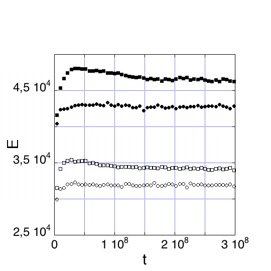
Figure 4: Energy distribution E as a function of time $t$. Geometric occupation volume: $6.4\%$. Circles: $N=25$, squares: $N=200$. Blank: $l_{p}=1$, solid: $l_{p}=1.5$.

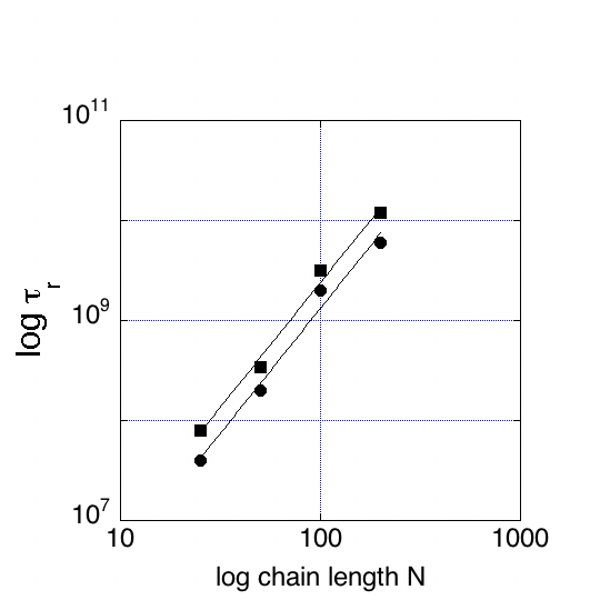
Figure 5: Relaxation time $\tau_{r}$ vs chain length $N$ on a logarithmic scale. Geometric occupation volume: $6.4\%$. The solid line is a power law fit with an exponent of 2.5. Squares: $l_{p}=1$, circles: $l_{p}=0.5$.

a

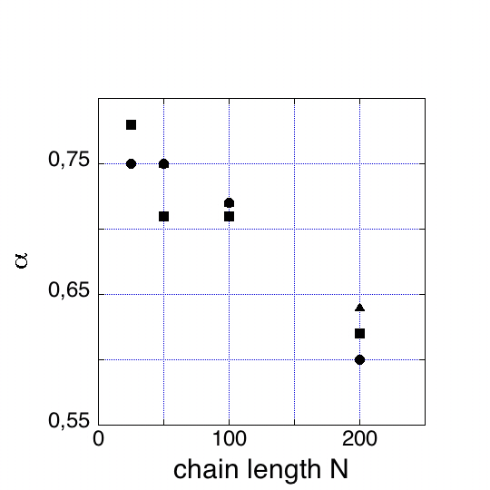
b

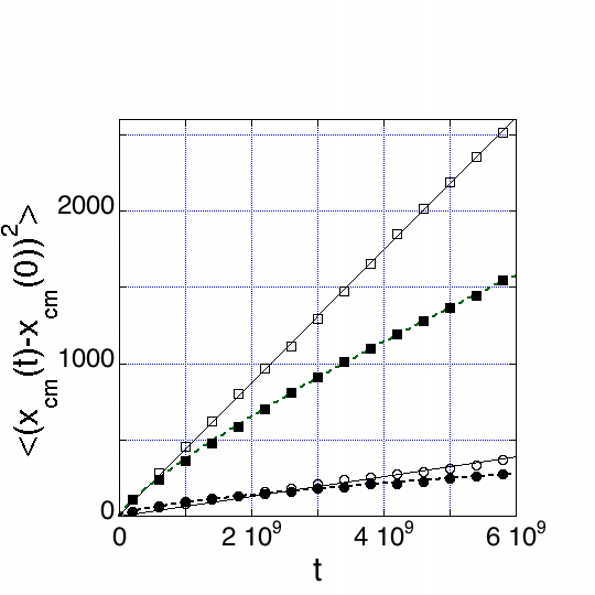
Figure 6: Upper panel: Anomalous translational diffusion exponent $\alpha$ as a function of chain length $N$. Geometric occupation volume: $6.4\%$. Circles: $l_{p}=1.5$, squares: $l_{p}=1$, triangles: $l_{p}=0.5$. Lower panel: Center of mass $\left\langle(x_{cm}(t)-x_{cm}(0))^{2}\right\rangle$ vs. time $t$. Squares: $N=25$, $l_{p}=0.5$, circles: $N=200$, $l_{p}=0.5$. Solid: $100\times 100\times 100$ cubic lattice, blank: $500\times 500\times 500$ cubic lattice. Straight line: linear fit, dashed line: power law fit.

IV.3.3 Particle diffusion in various environments

The initial position was randomly sampled inside the lattice, avoiding occupied lattice sites. Random walks of short times, 600 time steps, and long times, 200000 time steps, were carried out. This procedure was repeated over 5000 times and the data were averaged. The occupation volume was varied between 6.4% and 12.5%.

a

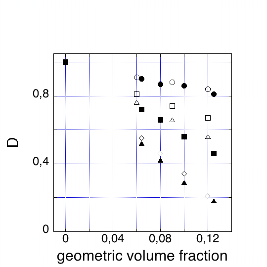
b

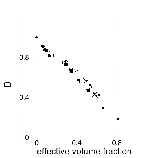
Figure 7: Comparison of the random walk chain model and the self avoiding random walk chain model. Upper panel: Diffusion coefficient dependent on the geometric volume fraction. Lower panel: Diffusion coefficient dependent on the effective volume fraction. Blank: Random walk chain model. Solid: Self avoiding random walk chain model. Diamonds: middle sized particle in the test system. Circles: smallest particle, squares: middle sized particle, and triangles: largest particle. Stars: largest particle in the SAW system with different persistence lengths $l_{p}$ of 0.5, 1, 2 and 3 with constant geometric occupation volume of $6.12\%$, respectively. Crosses: largest particle in the SAW system with different persistence lengths $l_{p}$ of 0.5, 1, 2 and 3 with constant geometric occupation volume of $7.95\%$, respectively.

Figure 7 displays the dependence of the diffusion coefficient on the geometric occupation volume and the walker size (solid symbols). Similar to the RW simulations (blank symbols) and the test system using disconnected obstacles (diamonds), a linear dependence of the diffusion coefficient on the effective occupation volume is found. Again, particles of larger size displayed a slower diffusion (upper panel), but additionally a clear separation regarding the environment is visible: Using RW chains, the particle was diffusing faster compared to SAW chains of identical (geometric) occupation volume. Slowest diffusion was observed using the test system of entirely disconnected obstacles (diamonds, only data for the medium sized particle are shown).

The reason for this separation: A SAW leads to a rather homogeneous chain distribution, due to the excluded volume interaction, when compared to the uncorrelated RW chain. Disconnected obstacles are even more randomly distributed. This is affecting the distribution of pore sizes and hence percolation paths through unoccupied lattice points. In particular, a random walker of large size is more restricted inside the SAW environment than inside the RW fibers, the latter offering large density fluctuations and hence larger connected pores of free space.

Again, these differences were properly accounted for after rescaling with respect to the effective volume fraction of the chains (Fig.  7, lower panel). Now, all data roughly fell onto a single master curve (lower panel). This result indicates that, in fact, different chain densities and conformations affect particle diffusion, but these subtle differences can be projected into a single parameter, the effective volume fraction.

A variation of the chain length of sufficiently long chromatin fibers ($N\in\{50,250,500\}$), while keeping the occupation volume constant, did not affect the diffusion coefficient of the walker. However, once shorter fibers were involved, with $N<50$, a reduction of $D$ was observed (Fig. 8, upper panel). Here we are approaching the limit of disconnected obstacles ($N=1$) which was discussed above.

Next, simulations were carried out with 46 long fibers of length $N\in\{10^{3},11^{3},12^{3}\}$, similar to chromatin fiber territories inside the cell nucleus (Fig.  3). Here, the persistence length $l_{p}$ was modified in order to study how particle diffusion is influenced by local variations of the fiber conformations. It was found that the diffusion of the smallest particle was not affected by the persistence length (Fig. 8, lower panel). A larger random walker, however, was slowing down with increasing persistence length.

Furthermore, we observed that the effective volume of the fiber network changed with different persistence lengths. After rescaling with respect to the effective volume fraction of the chains, the data, diffusion coefficients dependent on different $l_{p}$, fell on the master curve (Fig. 7, lower panel, crosses, stars). This implies that there are many parameters influencing the particle diffusion such as chain density, conformation and persistence length, but these parameters can be reduced to a single one, the effective volume.

a

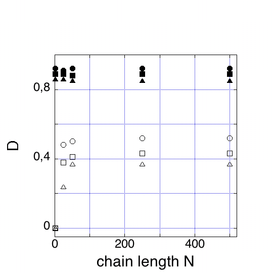
b

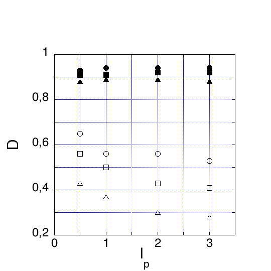
Figure 8: Upper panel: Diffusion coefficient as a function of chain length $N$ for different occupation volumes. Solid symbols: smallest particle. Blank symbols: largest particle. Circles denote 6.4% occupation volume, squares 8% occupation volume, and triangles 10% occupation volume. Lower panel: Diffusion coefficient as a function of persistence length $l_{p}$ for different occupation volumes. Circles: 46 chains with $N=1000$ (4.6% occupation volume), squares: 46 chains with $N=1331$ (6.12% occupation volume), triangles: 46 chains with $N=1728$ (7.95% occupation volume).

V Summary

It is a well known, if not trivial, wisdom that the complexity of biological systems requires drastic approximations in order to become feasible for numerical simulations. The question is: Which approximations?

The present work was intended to shed some light on the numerical modelling of diffusion processes inside the cell nucleus. First of all we have demonstrated that such a process can be described with a lattice model of the nucleus, the fibers and the random walk of the protein. The validity of this approach was checked using a straight comparison with the corresponding continuum model. Even though the treatment of a living system via lattice model may impose a cultural shock to some biologists, the benefits of having a finite number of states and, with the BFM, a highly efficient technique to simulate chains at any density, deliver a substantial speed-up without any apparent loss of accuracy.

To create a crowded environment of chromatin fibers in the cell nucleus, three different models were tested, yielding different structural properties of the chains. One of them was made of randomly distributed and disconnected obstacles, the second one a RW chain (in discrete and continuous space) and finally the rather realistic SAW chain model with excluded volume and persistence length.

In several systematic simulations, including walkers of various sizes, it was shown that conformational variations of the crowded environment led to visible modifications of the diffusion coefficients. First of all, and trivially, a larger occupation volume was slowing down the diffusion of all walkers. Moreover, it was found that, the more homogeneous the obstacles were distributed, the lower were the observed diffusion coefficients, in particular if the walker was of large size. Non-interconnected obstacles are more homogeneous than SAW chains, which in turn are more homogeneous than RW chains.

These effects could be accounted for with the concept of effective occupation volume of the system: This quantity is a convolution of geometric chain volume with the walker’s size, i.e. the effective free space available to the walker. Different chain models create different distributions of the pores (which form the free space available to the walker), even if the total chain volume remains unaffected. A modification of the walker size then effectively selects the available set of percolation paths through the dense network and hence its diffusion speed. Once the diffusion coefficient was plotted as a function of effective volume, the data fell onto a master curve, i.e. the effect of conformational variations on the diffusion could be eliminated. Towards the high end of effective chain volume, around 75%, the onset of subdiffusion was observed in all models (Fig. 2). The percolation threshold in case of bondless occupation of sites for a three-dimensional cubic lattice is well known, $p_{c}=0.31$ (see for instance Strenski et al. percolation). Thus, in our system, subdiffusion is visible when the occupation is slightly above the percolation threshold. We suspect that in a much larger system without finite size effects, and for much longer simulation times, we could also observe subdiffusion for occupation volumes closer to the percolation threshold.

In a similar manner, the persistence length of SAW chains did influence the chain distribution, which exhibited rather strong density fluctuations in case of highly flexible chains. Again, a scaling with the effective volume of the system allowed to eliminate these conformational variations on the diffusion behavior, and the data were falling onto the same master curve.

As a side aspect we observed that the translational diffusion of polymer chains in the investigated volume range was anomalous as a result of boundary restrictions of the cell. Once the space became practically unlimited, the translational diffusion coefficient decreased roughly inversely proportional to the chain length, as is to be expected when considering Rouse diffusion. It is not yet clear to which extent the experimentally observed slowing of DNA diffusion was caused by binding or by crowding (entanglement) effects slowdown. We believe that the model presented here is feasible to clarify these questions with the help of further systematic simulations.

VI Acknowledgement

A.W. thanks H.M. and C.W. for their hospitality during a research stay at the Department of Physics at the Xiamen University. A.W. was supported by a scholarship from the International PhD program of the German Cancer Research Center.