Semiclassical initial value calculations of the collinear helium atom

Abstract

Semiclassical calculations using the Herman-Kluk initial value treatment are performed to determine energy eigenvalues of bound and resonance states of the collinear helium atom. Both the $eZe$ configuration (where the classical motion is fully chaotic) and the $Zee$ configuration (where the classical dynamics is nearly integrable) are treated. The classical motion is regularized to remove singularities that occur when the electrons collide with the nucleus. Very good agreement is obtained with quantum energies for bound and resonance states calculated by the complex rotation method.

I Introduction

The inability of the old quantum theory to determine the energy spectrum of helium was one of the factors motivating the development of modern quantum mechanics. With the advent of the modern theory, attempts to treat helium within a classical framework continued with the application of semiclassical methods, obtained from an asymptotic analysis of the Schrödinger equation.Tanner00 . These studies eventually identified two key reasons for the failure of old theory’s attempts to describe the energy levels of this atom: the absence of the Maslov index in the older work,Leopold80 and the largely chaotic nature of the classical electronic dynamics in this system.Richter90 ; Blumel92 Due to this last factor, truly satisfactory semiclassical treatments had to await development of techniques for the quantization of chaotic motion. The first modern semiclassical calculations to properly account for the chaotic dynamics in helium appeared in the early 1990’s.Ezra91 ; Wintgen92 These and subsequent works have enabled the quantization of a large number of bound and resonance states of the atom.Tanner00 ; Ezra91 ; Wintgen92 ; Rost97 ; Wintgen94

Although other restricted-configuration coplanar studies have been carried out,Grujic95 most recent semiclassical treatments are based on a collinear model for the classical motion of the electrons, with corrections added for stable motion in the remaining degrees of freedom.Tanner00 Collinear helium can exist in two configurations:

• The $eZe$ configuration, characterized by the two electrons on different sides of the nucleus. This configuration is relevant for quantization of bound and resonant states of the three-dimensional atom with maximal positive values of the Stark quantum number $K$ including, apparently, the ground state of the atom. The classical motion for this configuration is believed to be completely chaotic, i.e., the periodic orbits are all linearly unstable and proliferate exponentially with orbit length. Semiclassical quantization in this case was performed by a periodic orbit cycle expansion technique.Ezra91 ; Wintgen92 ; Rost97

• The $Zee$ configuration, characterized by the two electrons on the same side of the nucleus. This configuration is implicated in the quantization of certain resonance states with maximal negative values of $K$. In strong contrast to the $eZe$ case, the classical behavior for the $Zee$ configuration is nearly integrable, with invariant tori centered about a stable periodic orbit describing the so-called ”frozen planet” motion.Richter92b Quantization for this case was achieved by applying the Einstein-Brillouin-Keller (EBK) treatment.Wintgen94 ; Richter90b ; Richter91

The justification for treating helium with reduced dimensionality is that many highly excited quantum states are dominated by the classical collinear motion. This conclusion rests on three arguments:Tanner00 (a) A scaling analysis shows that the classical dynamics of helium with total orbital angular momentum ${\bf L}$ at energy $E$ is equivalent to the dynamics of the system with angular momentum $|E|^{1/2}\mathbf{L}$ at energy $-1$. Thus, as the energy approaches the double ionization limit $E=0$, the classical motion relevant for states with low and moderate angular momentum quantum numbers becomes that for ${\bf L}=0$, which restricts the three particles to a plane. (b) It is known that the collinear $eZe$ and $Zee$ configurations form invariant subspaces in the full-dimensional phase space. (c) It can be shown that the collinear motion is stable with respect to bending deformations perpendicular to the linear configuration. On the basis of these arguments many states of the three-dimensional atom are expected to be structured about the backbone of collinear classical motion. This reduction in dimensionality was crucial for the ability to quantize states associated with the $eZe$ configuration since it enabled a thorough study and coding of the system’s periodic orbits.

Although the existing semiclassical treatments quite successfully reproduce energy levels for many states of the three-dimensional atom, full-dimensional calculations of helium are highly desirable. One problem with the collinear treatments is that they are applicable only to states with near-extreme values of the Stark quantum number; they are not truly appropriate for more general states. A second limitation of these approaches is they are not strictly justified for low-lying excited states of the atom where the arguments favoring collinearity, or even coplanarity, break down. This comment applies even to $S$ states which should, arguably, be treated semiclassically with nonzero $\mathbf{L}$ due to the Langer correction.Manning94 One consequence is that the accuracy of the semiclassical approximation for the ground state of helium has not yet been definitively established. Unfortunately, the semiclassical methods that have been used to quantize the chaotic classical motion for collinear $eZe$ helium cannot be easily applied to higher-dimensional systems where the dynamics generally have a mixed chaotic-regular nature and where a systematic search and characterization of all periodic orbits becomes unfeasible. Clearly, this limitation also blocks extension of these semiclassical techniques to atomic and molecular systems having more than two electrons. Thus, it is important to develop other semiclassical approaches that are capable of treating higher-dimensional many-electron systems.

Semiclassical initial value representation (IVR) methodsHerman84 ; Kluk86 ; Miller06 ; Thoss04 ; Kay05 are natural candidates for this role since they are capable of semiclassically propagating wave functions for systems with many degrees of freedom. Here we test the applicability of one such method for the quantization of many-body Coulombic systems by applying it to the collinear helium atom. In contrast to much of the previous semiclassical work for this system, no corrections for the motion perpendicular to the linear configuration are incorporated in the present treatment, so that the results apply to the collinear system only, not to the three-dimensional atom.

Although IVR treatments have been previously applied to single-electron systemsKay05 ; VandeSand99 ; Yoshida04 ; Takatsuka06 , the present application to a system with two electrons is nontrivial. The most serious difficulty concerns the strongly chaotic nature of the classical motion for the $eZe$ configuration. It is well established that such behavior creates numerical convergence difficulties in the propagation of systems by IVR methods beyond very short times.Kay94c ; Walton96 ; Spanner05 Thus, calculations for times long enough to extract quantization information are expected to be challenging. A related problem is associated with the classical instability of the helium atom with respect to ionization. In contrast to the quantum system, the classical atom can autoionize at all energies, even those below the first ionization limit. Thus, in general, one electron of the atom escapes to infinity after a few revolutions, leaving a bound He⁺ ion. This is an extreme example of the zero-point energy problemMiller89 ; Bowman89 that plagues classical trajectory simulations of quantum evolution. More specifically, the potential difficulty in the present context arises from the reliance of IVR methods on general classical trajectories that are almost never true periodic orbits. Quantization is obtained from those trajectories that shadow the periodic orbits for long time intervals. The short lifetime of many trajectories, resulting from the classical autoionization, may require a drastic increase in the total number of trajectories that must be calculated. A final problem anticipated for IVR treatments of the collinear atom in both configurations (and one that is common to all numerical semiclassical calculations for these systems) arises because the electrons undergo repeated collisions with the nucleus, where the Coulombic interaction becomes infinite. At such collisions, the classical equations of motion become singular, and they cannot be integrated by ordinary methods. Numerical solution of the classical equations of motion for collinear helium thus requires regularization techniques.

The remainder of this paper is organized as follows. Section II presents the expressions that form the basis of the present treatment. Section III describes the semiclassical calculations, Sec. IV presents the numerical results, and Sec. V discusses and summarizes the main points of our work. An Appendix presents details of supporting quantum calculations for the energy levels of the collinear atom.

II Theory

In atomic units, the Hamiltonian for the collinear helium atom is given by

$$H=\frac{p_{1}^{2}}{2}+\frac{p_{2}^{2}}{2}-\frac{2}{q_{1}}-\frac{2}{q_{2}}+\frac{1}{|q_{2}\pm q_{1}|},$$ (1)

where ${\bf q}^{T}=(q_{1},q_{2})$ are the coordinates and ${\bf p}^{T}=(p_{1},p_{2})$ are the momenta of the two electrons. The $+$ and $-$ signs in the last term apply to the $eZe$ and $Zee$ configurations, respectively.

Here we wish to determine the energies of bound and resonance states for these two configurations. In a purely quantum calculation, such energies can be extracted from peaks in the spectrum

$$F(E)=\left|\int_{0}^{\infty}\,\exp(iEt)\,c(t)\,dt\right|^{2}$$ (2)

where $c(t)$ is the autocorrelation function

$$c(t)=\int d\mathbf{r}^{\prime}\int d\mathbf{r}\,\Psi_{0}^{*}(\mathbf{r}^{\prime})K(\mathbf{r}^{\prime},\mathbf{r},t)\Psi_{0}(\mathbf{r}).$$ (3)

Here $\Psi_{0}$ denotes an initial state which projects onto energy eigenstates of interest and

$$K(\mathbf{r}^{\prime},\mathbf{r},t)=\langle\mathbf{r}^{\prime}|\exp(-i\hat{H}t)|\mathbf{r}\rangle$$ (4)

is the propagator, describing the time evolution operator in the representation of positions ${\bf r}^{T}=(r_{1},r_{2})$. In the present semiclassical calculations, this propagator is approximated semiclassically.

The specific semiclassical treatment used here is that of Herman and Kluk (HK)Herman84 ; Kluk86 who expressed the propagator in the IVR form

$$K^{HK}({\bf r}^{\prime},{\bf r},t)=\int\!\!\!\int\frac{\mathrm{d}^{2}q\,\mathrm{d}^{2}p}{(2\pi)^{2}}\,\langle{\bf r}^{\prime}|{\bf q}_{t},{\bf p}_{t}\rangle\,R_{{\bf q}{\bf p}t}\,\exp(iS_{{\bf q}{\bf p}t})\,\langle{\bf q},{\bf p}|{\bf r}\rangle,$$ (5)

where the integrals are over momenta $\mathbf{p}$ and coordinates $\mathbf{q}$ that serve as initial conditions for classical trajectories. The trajectories carry these phase space variables at time 0 to values $(\mathbf{p}_{t},\mathbf{q}_{t})$ at time $t$. The quantities

$$\langle{\bf r}|{\bf q},{\bf p}\rangle=\left(\frac{\textrm{det}\bm{\gamma}}{\pi^{2}}\right)^{1/4}\exp\left[-\frac{1}{2}({\bf r}-{\bf q})^{T}\bm{\gamma}({\bf r}-{\bf q})+i{\bf p}^{T}({\bf r}-{\bf q})\right]$$ (6)

are Gaussian coherent state functions. $\bm{\gamma}$ is a $2\times 2$ diagonal matrix with real nonzero elements $\gamma_{1},\gamma_{2}$ which determine the Gaussian widths along $r_{1}$ and $r_{2}$. The function $S_{{\bf q}{\bf p}t}=\int_{0}^{t}\mathrm{d}t^{\prime}(\mathbf{p}_{t^{\prime}}\dot{\mathbf{q}}_{t^{\prime}}-H)$ is the action along the trajectory and the prefactor $R_{{\bf q}{\bf p}t}$ has the form

$$R_{{\bf q}{\bf p}t}=\left\{{\textrm{det}\left[\frac{1}{2}\left(\frac{\partial{\bf q}_{t}}{\partial{\bf q}}+\bm{\gamma}^{-1}\frac{\partial{\bf p}_{t}}{\partial{\bf p}}\bm{\gamma}-i\frac{\partial{\bf q}_{t}}{\partial{\bf p}}\bm{\gamma}+i\bm{\gamma}^{-1}\frac{\partial{\bf p}_{t}}{\partial{\bf q}}\right)\right]}\right\}^{1/2},$$ (7)

where each term under the radical is a $2\times 2$ block of the 4-dimensional monodromy matrix defined by

$$\left(\begin{array}[]{c}\delta{\bf q}_{t}\\ \delta{\bf p}_{t}\end{array}\right)=\left(\begin{array}[]{cc}\partial{\bf q}_{t}/\partial{\bf q}&\partial{\bf q}_{t}/\partial{\bf p}\\ \partial{\bf p}_{t}/\partial{\bf q}&\partial{\bf p}_{t}/\partial{\bf p}\end{array}\right)\left(\begin{array}[]{c}\delta{\bf q}\\ \delta{\bf p}\end{array}\right).$$ (8)

A potential difficulty with applying the HK propagator in the present case is that (5) is technically valid only for systems with wave functions that obey boundary conditions at $r_{i}=\pm\infty$. In contrast, the wave functions of collinear helium are required to obey boundary conditions at $r_{i}=0$ (where they must vanishBlumel92 ). Due to the Gaussian form of the functions $\langle{\bf r}^{\prime}|{\bf q}_{t},{\bf p}_{t}\rangle$, the wave functions calculated using the HK treatment will not satisfy this property. To remedy this problem, the IVR expression for the propagator should be modified to replace the Gaussian coherent state functions with certain functions that vanish at $r_{i}=0$ and obey some additional requirements.Kay05 ; Kay01 . Fortunately, however, these modifications are not needed for the present calculations. The states $\Psi_{0}(\mathbf{r})$, which we use to prepare the system at time 0 and to probe the positions of the particles at times $t$, are localized in regions far from $r_{i}=0$. Thus, the initial states effectively obey the proper boundary conditions and the function $c(t)$ is insensitive to the behavior of the propagated wave functions $\Psi_{t}(\mathbf{r}^{\prime})=\int d\mathbf{r}K^{HK}(\mathbf{r^{\prime}},\mathbf{r},t)\Psi_{0}(\mathbf{r})$ near $r_{i}^{\prime}=0$. The results of an HK calculation should then be the same as for a modified IVR propagator in which the coherent state functions are replaced by new functions that are strongly non-Gaussian at $r_{i}=0$ (as needed to obey the boundary conditions) but become almost Gaussian far from the boundaries. This was confirmed by calculations in which the $\langle{\bf r}|{\bf q},{\bf p}\rangle$ and $\langle{\bf r}^{\prime}|{\bf q}_{t},{\bf p}_{t}\rangle$ were replaced by combinations of Gaussian coherent state functions which vanish at $r_{i}=0$. The results were essentially identical to those obtained with the ordinary HK expression.

As mentioned above, it is necessary to regularize the classical equations of motion because they become singular when electrons collide with the nucleus ($q_{1t}=0$ or $q_{2t}=0$) and cannot be integrated by applying ordinary numerical techniques. As a prelude to this regularization, it is convenient to transform the coordinates and momenta to scaled variables defined by

$$\tilde{q}_{i}=|E|q_{i},\qquad\tilde{p}_{i}=|E|^{-1/2}p_{i}\qquad(i=1,2)$$ (9)

where $E$ is the energy of the atom. In terms of these variables, the Hamiltonian can be expressed as $H=|E|\tilde{H}$ where

$$\tilde{H}=\frac{\tilde{p}_{1}^{2}}{2}+\frac{\tilde{p}_{2}^{2}}{2}-\frac{2}{\tilde{q}_{1}}-\frac{2}{\tilde{q}_{2}}+\frac{1}{|\tilde{q}_{2}\pm\tilde{q}_{1}|}$$ (10)

has an energy-independent value. For the present treatment of bound and resonance states (for which $E<0$) we set $\tilde{H}=-1$. The physical variables $(\mathbf{q}_{t},\mathbf{p}_{t})$ at time $t$ can be calculated by solving Hamilton’s equations of motion with Hamiltonian $\tilde{H}$ to obtain the scaled variables at the time $\tilde{t}$, defined by

$$\tilde{t}=|E|^{3/2}t,$$ (11)

and then applying (9).

To complete the regularization procedure, we apply a transformation similar to that proposed by Kustaanheimo and StiefelKustaanheimo65 ; Aarseth74 . In our case, this involves defining a new Hamiltonian $\mathcal{H}=\tilde{q}_{1}\tilde{q}_{2}(\tilde{H}+1)$ which is numerically equal to zero and is free from singularities. Introducing the regularized variables $(Q_{i},P_{i})$, defined via the equations

$$\tilde{q}_{i}=Q_{i}^{2}\qquad\tilde{p}_{i}=\frac{P_{i}}{2Q_{i}}\qquad(i=1,2),$$ (12)

$\mathcal{H}$ takes the form

$$\mathcal{H}=\frac{(Q_{2}^{2}P_{1}^{2}+Q_{1}^{2}P_{2}^{2})}{8}-2(Q_{1}^{2}+Q_{2}^{2})+Q_{1}^{2}Q_{2}^{2}+\frac{Q_{1}^{2}Q_{2}^{2}}{|Q_{2}^{2}\pm Q_{1}^{2}|}.$$ (13)

With this Hamiltonian, the classical equations of motion for $dQ_{i\tau}/d\tau$ and $dP_{i\tau}/d\tau$ are solved with initial conditions $(Q_{i},P_{i})$ at time 0 to determine values of $(Q_{i\tau},P_{i\tau})$ as a function of a new time variable $\tau$. This variable is related to the scaled time $\tilde{t}$ by the differential equation

$$\frac{d\tilde{t}}{d\tau}=Q_{1\tau}^{2}Q_{2\tau}^{2},$$ (14)

which must be integrated along with Hamilton’s equations. The physical variables $p_{it},q_{it}$ at time $t$ are then obtained by reversing the regularization and scaling transformations.

The physical action integral $S_{t}$ needed to form the HK integrand can be obtained from the regularized variables by applying

$$S_{t}=|E|^{-1/2}{\mathcal{S}}_{\tau},$$ (15)

where the scaled action ${\mathcal{S}}_{\tau}$ is determined by integrating the equation

$$\frac{d{\mathcal{S}}_{\tau}}{d\tau}=\frac{(Q_{2\tau}^{2}P_{1\tau}^{2}+Q_{1\tau}^{2}P_{2\tau}^{2})}{8}+2(Q_{1\tau}^{2}+Q_{2\tau}^{2})-\frac{Q_{1\tau}^{2}Q_{2\tau}^{2}}{|Q_{2\tau}^{2}\pm Q_{1\tau}^{2}|}.$$ (16)

To evaluate the monodromy elements needed for the semiclassical calculation, we begin with the relations

$$|E|\,q_{it} = Q_{i\tau}^{2},$$

$$2\,Q_{i\tau}\,p_{it} = \sqrt{|E|}\,\,P_{i\tau},$$ (17)

which are obtained by combining (9) and (12). Treating $(Q_{i\tau},P_{i\tau})$ as functions of $t$ and the initial conditions $\alpha=\{q_{1},q_{2},p_{1},p_{2}\}$, and taking partial derivatives with respect to any one of these variables, $\alpha_{j}$, we obtain

$$|E|\,\frac{\partial q_{it}}{\partial\alpha_{j}} = 2\,Q_{i\tau}\,\left(\frac{\partial Q_{i\tau}}{\partial\alpha_{j}}\right)_{t}-q_{it}\frac{\partial|E|}{\partial\alpha_{j}},$$

$$Q_{i\tau}\,\frac{\partial p_{it}}{\partial\alpha_{j}} = -p_{it}\,\left(\frac{\partial Q_{i\tau}}{\partial\alpha_{j}}\right)_{t}+\frac{\sqrt{|E|}}{2}\,\left(\frac{\partial P_{i\tau}}{\partial\alpha_{j}}\right)_{t}+\frac{P_{i\tau}}{4\sqrt{|E|}}\,\frac{\partial|E|}{\partial\alpha_{j}}.$$ (18)

To determine the partial derivatives of $Q_{i\tau}$ and $P_{i\tau}$ with respect to $\alpha_{j}$ appearing above, we treat $Q_{i\tau}$ and $P_{i\tau}$ as functions of the initial values $Q_{i},P_{i}$ and of $\tau$. Differentiating with respect to $\alpha_{j}$ and applying the equations of motion then gives

$$\left(\frac{\partial Q_{i\tau}}{\partial\alpha_{j}}\right)_{t} = \frac{\partial Q_{i\tau}}{\partial Q_{k}}\,\frac{\partial Q_{k}}{\partial\alpha_{j}}+\frac{\partial Q_{i\tau}}{\partial P_{k}}\,\frac{\partial P_{k}}{\partial\alpha_{j}}+\frac{\partial\mathcal{H}}{\partial P_{i\tau}}\,\left(\frac{\partial\tau}{\partial\alpha_{j}}\right)_{t},$$

$$\left(\frac{\partial P_{i\tau}}{\partial\alpha_{j}}\right)_{t} = \frac{\partial P_{i\tau}}{\partial Q_{k}}\,\frac{\partial Q_{k}}{\partial\alpha_{j}}+\frac{\partial P_{i\tau}}{\partial P_{k}}\,\frac{\partial P_{k}}{\partial\alpha_{j}}-\frac{\partial\mathcal{H}}{\partial Q_{i\tau}}\,\left(\frac{\partial\tau}{\partial\alpha_{j}}\right)_{t}.$$ (19)

Finally, to determine $(\partial\tau/\partial\alpha)_{t}$ in the above equations, we differentiate $\tilde{t}$ (considered as a function of initial conditions and $t$) with respect to $\alpha_{j}$ and apply (11) and (14). This yields

$$\frac{3}{2}\,\sqrt{|E|}\,\frac{\partial|E|}{\partial\alpha_{j}}\,t=\frac{\partial\tilde{t}}{\partial Q_{k}}\,\frac{\partial Q_{k}}{\partial\alpha_{j}}+\frac{\partial\tilde{t}}{\partial P_{k}}\,\frac{\partial P_{k}}{\partial\alpha_{j}}+Q_{1\tau}^{2}\,Q_{2\tau}^{2}\,\left(\frac{\partial\tau}{\partial\alpha_{j}}\right)_{t},$$ (20)

from which $(\partial\tau/\partial\alpha)_{t}$ can be obtained. These equations thus express the physical monodromy matrix in terms of the regularized monodromy matrix and the partial derivatives $\partial\tilde{t}/\partial Q_{k}$ and $\partial\tilde{t}/\partial P_{k}$. The various quantities needed to calculate the physical monodromy matrix can now be formed by solving a set of first-order ordinary differential equations in the variable $\tau$, obtained by differentiating Hamilton’s equations (for $dQ_{i\tau}/d\tau$ and $dP_{i\tau}/d\tau$) and (14) (for $d\tilde{t}/d\tau$) with respect to $Q_{k}$ and $P_{k}$.

We mention that an alternative procedure for calculating the physical monodromy matrix can be formulated in terms of a transformation to so-called local coordinatesRichter93 . However, the present approach was adopted here since numerical tests showed that it allows larger time steps for the integration of the differential equations.

Note that the differential equations that are solved here remain well behaved for all values of $\tau$. The singularities in the physical variables (monodromy elements and momenta), occurring at collisions with the nucleus, arise only from (II)-(20), describing transformations from the regularized variables. Nevertheless, such singularities cause the prefactor $R_{{\bf q}{\bf p}t}$ to behave as $q_{it}^{-1}$ for $q_{it}\to 0$, raising the suspicion that the HK integral diverges for the present system. Fortunately, these singularities in $R_{{\bf q}{\bf p}t}$ are cancelled by factors such as $\exp[-(p_{it}-p_{i0})^{2}/4\gamma_{i}]$ appearing in the expressions for $c(t)$ [see (23) below], which cause the HK integrand to vanish when $q_{it}\to 0$ since $p_{it}\propto q_{it}^{-1/2}$ in such cases.

While the regularization presented above provides a unique continuation of the classical equations of motion when one of the coordinates $q_{1t}$ or $q_{2t}$ becomes zero (a binary collision), no unique continuation exists when both $q_{1t}$ and $q_{2t}$ become zero simultaneously (a triple collision). Fortunately, the initial collisions leading to an exact triple collision form a set of zero measure in the system’s phase space and do not contribute to calculations of the HK propagator.

III semiclassical calculations

The symmetry of the Hamiltonian in (1) implies that two distinct kinds of energy eigenstates exist: states that are symmetric with respect to electron exchange (which can be identified with singlet spin states) and states that are antisymmetric with respect to electron exchange (which can be identified with triplet spin states). As in the case of exact quantum evolution, one expects that energy spectra for the two kinds of states can be obtained separately by semiclassically propagating initial states of definite exchange symmetry. Thus, in our calculations, we choose the functions $\Psi_{0}$ in (3) to have the (anti)symmetrized form

$$\Psi_{0}(\mathbf{r})={\mathcal{N}}\left[\langle r_{1}|q_{10},p_{10}\rangle\langle r_{2}|q_{20},p_{20}\rangle\pm\langle r_{1}|q_{20},p_{20}\rangle\langle r_{2}|q_{10},p_{10}\rangle\right],$$ (21)

where $\langle r_{i}|q_{j0},p_{j0}\rangle$ are one-dimensional Gaussian coherent state functions involving parameters $(q_{j0},p_{j0})$ and ${\mathcal{N}}$ is a normalization constant. We choose the values of $\gamma_{j}$ for these functions to be equal to those used to construct the functions $\langle{\bf r}|{\bf q},{\bf p}\rangle=\langle r_{1}|q_{1},p_{1}\rangle\langle r_{2}|q_{2},p_{2}\rangle$ in the propagator. However, rather than propagate a combination of coherent state functions, it is more convenient to propagate a single, unsymmetrized, “initial” state and project out the desired symmetry component with a properly symmetrized “final” state.Kay94c Applied to the autocorrelation function [(3)], this treatment yields

$$c^{HK}(t)=2{\mathcal{N}}^{2}\int\!\!\!\int\frac{\mathrm{d}^{2}q\,\mathrm{d}^{2}p}{(2\pi)^{2}} \left[\langle q_{10},p_{10}|q_{1t},p_{1t}\rangle\langle q_{20},p_{20}|q_{2t},p_{2t}\rangle\pm\langle q_{20},p_{20}|q_{1t},p_{1t}\rangle\langle q_{10},p_{10}|q_{2t},p_{2t}\rangle\right]$$ (22)

$$R_{{\bf q}{\bf p}t}\exp(iS_{{\bf q}{\bf p}t})\langle q_{1},p_{1}|q_{10},p_{10}\rangle\langle q_{2},p_{2}|q_{20},p_{20}\rangle.$$

The product of overlap factors on the extreme right in (22) can be expressed in the analytical form

$$\langle{\bf q},{\bf p}|{\bf q}_{0},{\bf p}_{0}\rangle= \exp\left[-\frac{1}{4}({\bf q}-{\bf q}_{0})^{T}\gamma({\bf q}-{\bf q}_{0})-\frac{1}{4}({\bf p}-{\bf p}_{0})^{T}\gamma^{-1}({\bf p}-{\bf p}_{0})\right]$$ (23)

$$\times\exp\left[\frac{i}{2}({\bf p}+{\bf p}_{0})^{T}({\bf q}-{\bf q}_{0})\right].$$

In our calculations, we used the Gaussian distribution, formed from the modulus of this expression, to sample points in phase space for a Monte Carlo evaluation of the integrals over $(\mathbf{q},\mathbf{p})$ in (22).

To calculate the integrand in (22), the transformations (9) and (12) were applied to determine values for the regularized variables $Q_{i},P_{i}$ for each physical point $(\mathbf{q},\mathbf{p})$ sampled. Using these as initial conditions, Hamilton’s equations for $Q_{i\tau}$ and $P_{i\tau}$ were solved numerically, along with (14) and (16), as well as the $\tau$-dependent differential equations for elements [e.g. $\partial Q_{i\tau}/\partial Q_{j}$] of the regularized monodromy matrix and the quantities $\partial\tilde{t}/\partial Q_{i}$, $\partial\tilde{t}/\partial P_{i}$. This set of 26 equations was integrated using a variable stepsize Runge-Kutta methodPress92 . The values of $\tau$, corresponding to an evenly-spaced sequence of desired times $t$, were determined by a root-solving procedure and, at such times, the transformations were reversed to obtain the physical coordinates, momenta, action, and monodromy elements, needed for construction the integrand.

The final step in the calculation, namely, the evaluation of the Fourier transform in (2), was performed by the harmonic inversion procedure,Wall95 ; Mandelshtam97a ; Mandelshtam97b which effectively fits the computed autocorrelation function to an expression of the form

$$c^{HK}(t)=\sum_{k}d_{k}\exp(-iE_{k}t),$$ (24)

extracting values for the complex parameters $E_{k}$ and $d_{k}$. This method was preferred over ordinary Fourier transform techniques since it was capable of producing spectra of higher resolution spectra from our autocorrelation data, which were calculated for relatively short time durations.

Numerical difficulties, caused by the highly chaotic nature of the classical dynamics for the $eZe$ configuration, made it necessary to apply some additional approximations. As is well known, the chaotic motion causes the modulus of the HK prefactor $R_{{\bf q}{\bf p}t}$ to increase approximately exponentially with time.Kay94c ; Walton96 ; Spanner05 This systematic increase is distinct from singularities in the prefactor that occur when an electron collides with the nucleus. In principle, chaos should also cause the phases in the HK integrand to vary rapidly as a function of initial condition and the resulting cancellations should compensate for the growth of the prefactor, reducing the autocorrelation function to physically correct values. However, as time progresses, the prefactor becomes so large that the number of Monte Carlo-sampled trajectories needed for this cancellation exceeds practical limits. As a result, the calculation cannot be made to converge beyond a short time. The practice of discarding trajectories with large prefactorsKay94c ; Spanner05 does not, by itself, solve this problem for the present system since, to achieve convergence, it is necessary to eliminate almost all trajectories that do not autoionize.

To reduce the severity of this difficulty we observe that it is the phase of the prefactor, rather than its modulus, that is primarily responsible for creating the interference in the phase space integration which results in quantization. Thus, as other works demonstrate,Kaledin03a ; Kaledin03b ; Takatsuka07 it is possible to improve numerical convergence of the autocorrelation expression (without adversely affecting the computed energies) by replacing the modulus of the prefactor with a less rapidly increasing function of time, while retaining the accurate value of the phase. The choice for this replacement is not very critical, but a constant value for $|R_{{\bf q}{\bf p}t}|$ is found not to work well here since the rapidly varying integrand phases then cause the resulting autocorrelation signal to decay too quickly. In the present work, we have found it useful to replace the computed value of $|R_{{\bf q}{\bf p}t}|$ with $|R_{{\bf q}{\bf p}t}|^{1/2}$.

Despite this step, we still find it necessary to discard a very small minority of trajectories (e.g., about one trajectory out of $10^{5}$) having extremely large prefactors (e.g., $|R_{{\bf q}{\bf p}t}|>10^{20}$) which would otherwise destroy the numerical convergence of the calculations. We emphasize that the above steps were used only for the calculations of the $eZe$ configuration. For calculations of the nonchaotic $Zee$ configuration, the correct HK expressions for the prefactors were used and no trajectories were discarded due to large $|R_{{\bf q}{\bf p}t}|$,

One final simplification adopted here was to filter out trajectories with energies sufficiently far from the average energy of the initial state $\Psi_{0}$ and the target energy eigenvalues. Thus, trajectories with positive energies (above the double ionization limit) and sufficiently negative energies were eliminated from the phase space integrations. Removal of trajectories with low energies was especially important for the $eZe$ configuration since they become highly unstable at relatively short times, leading to very large prefactors, and making it difficult to achieve convergence for the required time durations.

IV results

As in the case of the three dimensional helium atom, the $eZe$ and $Zee$ collinear systems have bound, resonance, and continuum states. We denote bound and resonance states with the symbol $N_{n}$ where $N=1,2,\ldots$ and $n=N,N+1,\ldots$ are, respectively, approximate quantum numbers for the inner electron and outer electrons. For each $N$, the states $N_{n}$ form a Rydberg series converging, as $n\to\infty$, to an ionization threshold with energy $E=-2/N^{2}$ a.u. The series associated with $N=1$ ($E<-2.0$ a.u.) are bound states while those associated with $N>1$ are resonances.

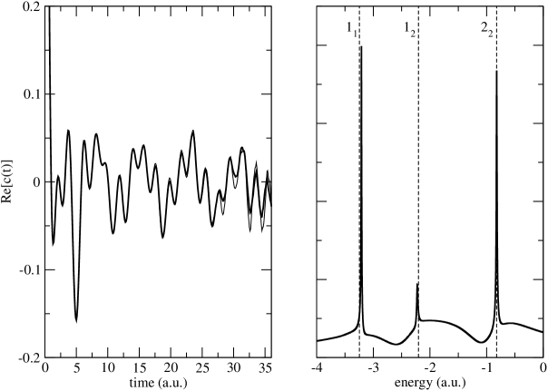
Figure 1: Results obtained for the $eZe$ configuration with the initial state having parameters ${\bf q}_{0}^{T}=(2.0,2.0)$, ${\bf p}_{0}^{T}=(0,0)$ and $\gamma_{1}=\gamma_{2}=1.0$ a.u. The left panel shows the real part of autocorrelation functions calculated using about $2.3\times 10^{7}$ trajectories (heavy curve) and $1.1\times 10^{7}$ trajectories (light curve). The right panel shows the energy spectrum obtained by the harmonic inversion method. The vertical dashed lines indicate quantum levels.

Figure 1 shows the autocorrelation function and spectrum obtained for the $eZe$ configuration using an initial state with ${\bf q}_{0}^{T}=(2.0,2.0)$, ${\bf p}_{0}^{T}=(0,0)$ and $\gamma_{1}=\gamma_{2}=1.0$. This same state was previously used by SimonovićSimonovic04 in a quantum mechanical calculation of the autocorrelation function for this system. The spectrum obtained from that calculation had three visible peaks, corresponding to energies of the ground state $1_{1}$, the first excited state $1_{2}$, and the lowest resonance state $2_{2}$. The present semiclassical calculations with this initial state were performed using $2.3\times 10^{7}$ trajectories having energies between -3.5 and 0 a.u. The convergence of the resulting autocorrelation function can be judged by comparing the heavy curve in the left panel of figure 1 with the light curve, which was obtained using half the number of trajectories. The harmonic inversion spectrum shown in the right panel of figure 1 has peaks for the same three levels observed in the split propagator quantum calculation.Simonovic04 Also shown in the figure are vertical lines denoting quantum mechanical energies, computed by the complex rotation method (see Appendix A for details). The semiclassical-quantum agreement is seen to be good, even for the ground state

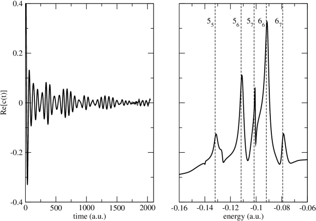
Figure 2: Results obtained for the $eZe$ configuration with the initial state having parameters ${\bf q}_{0}^{T}=(30.0,30.0)$, ${\bf p}_{0}^{T}=(0,0)$ and $\gamma_{1}=\gamma_{2}=0.1$. The left panel presents two curves for the real part of autocorrelation function that are difficult to resolve on the scale of the figure: a thick curve showing results obtained using about $3.6\times 10^{5}$ trajectories and a thin curve showing results obtained with about half this number of trajectories. The right panel shows the energy spectrum obtained by the harmonic inversion method. The vertical dashed lines indicate quantum levels.

Figure 2 presents further results for the $eZe$ configuration, obtained using an initial state with parameters ${\bf q}_{0}^{T}=(30.0,30.0)$, ${\bf p}_{0}^{T}=(0,0)$, and $\gamma_{1}=\gamma_{2}=0.1$. This state projects onto resonances which form the lowest members of the Rydberg series with $N=5$ and $N=6$. Well-converged calculations of the autocorrelation function were obtained using $3.6\times 10^{5}$ trajectories with energies between -4.0 and 0 a.u. No trajectories were discarded due to large prefactors. Agreement with quantum values is seen to be very good.

Results from these and additional, similar, calculations for singlet and triplet states of the $eZe$ configuration are displayed in Table 1. The semiclassical values reported are the real parts of the harmonic inversion parameters $-E_{k}$ of (24). Perhaps due to the reduction in the prefactor modulus, the imaginary parts of these parameters are usually about an order of magnitude larger than the quantum values, and are not reported here.

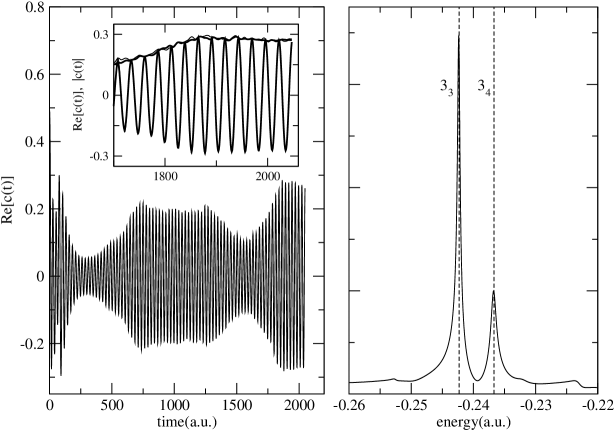
Figure 3: Results obtained for the $Zee$ configuration with the initial state having parameters ${\bf q}_{0}^{T}=(8.37,22.41)$, ${\bf p}_{0}^{T}=(0,0)$ and $\gamma_{1}=\gamma_{2}=0.4$. The left panel shows the real part of the autocorrelation functions. The inset shows details of the real part and modulus of $c(t)$ obtained with about $2.3\times 10^{6}$ trajectories (heavy curve) and $1.2\times 10^{5}$ trajectories (light curve). The right panel shows the energy spectrum obtained by the harmonic inversion method. The vertical dashed lines indicate quantum levels.

In our treatment of the $Zee$ configuration, lowest energy levels corresponding to $n=N$ and $n=N+1$ for specific Rydberg series $N$ were calculated by choosing the $(\mathbf{q}_{0},\mathbf{p}_{0})$ parameters of the initial states to coincide with the location of the central frozen planet orbit for this system. Since this orbit passes near the phase space point ${\bf q}_{0}^{T}=(2.15,5.76)$, ${\bf p}_{0}^{T}=(0,0)$ at $E=-1$,Richter92b the initial state for calculation of quantum states at an approximate energy $E$ was chosen to have parameters ${\bf q}_{0}^{T}=(2.15/|E|,5.76/|E|)$, ${\bf p}_{0}^{T}=(0,0)$. Figure 3 shows results obtained in this way with the estimate $E=-0.257$ a.u. and $\gamma_{1}=\gamma_{2}=0.4$. About $2.3\times 10^{6}$ trajectories with energies between $-3.0$ and $0$ a.u. were used to produce the convergent autocorrelation curve shown in this figure.

Results for these and other $Zee$ states, obtained in a similar way, are reported and compared to quantum energies in Table 2. Since, for this configuration, our semiclassical calculations yielded numerically identical energy levels for symmetric and antisymmetric states with $n>N$, only one set of energies is reported for each set of quantum numbers. It appears likely that the singlet-triplet splitting in these cases is due to tunnelling through the electron-electron repulsion barrier. It is known that the HK method is unreliable for treatment of such “deep” tunnelling phenomena.Kay05

V Discussion and Conclusion

Periodic orbit methods are superior tools for understanding how quantization emerges from classical behavior. However IVR techniques provide a way for performing semiclassical calculations that may remain practical even when the periodic orbit treatments are unfeasible. The results of this work show that the such methods can be successfully applied to systems with more than one electron.

Such applications are, however, not trivial. The Coulomb singularity, the high degree of chaos, and the instability of the classical dynamics characterizing these systems, significantly complicate the use of IVR methods. Nevertheless, these difficulties can be largely overcome, allowing calculation of converged autocorrelation signals for times that are long enough to quantize the systems treated. Among the methods used to achieve this were regularization of the motion, reduction of the modulus the HK prefactor, removal of trajectories with sufficiently negative energies, and application of the harmonic inversion method to form the autocorrelation spectrum.

The problems mentioned in the Introduction, concerning the classical autoionization of many-electron systems, turned out to be somewhat less serious than anticipated. The classical escape of electrons does require the calculation of additional trajectories, but the computational effort involved is partly offset by savings obtained by terminating trajectories once they ionize.

Agreement between the semiclassical results and quantum energies was generally very good. The semiclassical energies obtained for almost all bound and resonance states examined were within about 1% of the exact values. This accuracy was achieved even for the ground state of the $eZe$ configuration. We note that previous semiclassical treatments of this stateEzra91 ; Wintgen92 provide the current semiclassical estimates of the ground state energy for the three-dimensional atom.

In practice, even with the use of harmonic inversion, resolution of individual levels in the energy spectrum requires calculation of the autocorrelation function for longer times when the density of states increases. Since, for each $N$, this density becomes infinite as $n\to\infty$, IVR methods are not suitable for calculating levels with large values of $n-N$. However, as the energy increases ($|E|\to 0$), the scaling relation, (11), implies that IVR calculations can be continued for longer times without encountering significant problems due to chaos, autoionization, etc. The results obtained here demonstrate that this allows application of the IVR method to determine energies for the first few resonances of each Rydberg series $N$, even when $N$ is moderately large.

As stated in the Introduction, the present work is motivated by the possibility of performing semiclassical calculations for the fully three-dimensional helium atom and other atomic and molecular systems. Since the number of trajectories needed in the present calculations is already large, attempts to treat such systems would certainly benefit from improvements in the efficiency of the IVR technique. One way in which this can be accomplished is by exploiting the energy scaling of the classical motion more thoroughly. In the present work, separate trajectories were calculated for each physical initial condition sampled in the four-dimensional phase space. With an appropriate reformulation, it should be possible to achieve savings by running trajectories at a single energy only and scaling the results.Takatsuka06 A second way to increase the efficiency of the calculations is to replace integration over one of the remaining phase space variables with an integration over time along the trajectoriesElran99a ; Elran99b . Calculations for other systems show that this approach significantly reduces the number of independent phase space points which need to be sampled to obtain converged results. Still greater improvements can be often be achieved by applying a family of IVR methods which cut the dimensionality of the phase space integration by half.Sklarz04

Even without these modifications, the present HK treatment may prove to be successful for many states of the three dimensional helium atom. Since the motion perpendicular to the collinear configurations is known to be stable, it may perhaps be said that the present calculations for the $eZe$ configuration already treat the most problematic subspace of the three-dimensional system. Thus, application of IVR methods seem to place full-dimensional semiclassical calculations of atoms and molecules within reach.

Appendix A Quantum calculations

Energy levels for singlet states of the $eZe$ configuration were previously calculated quantum mechanically by Blümel and ReinhardtBlumel92 using the complex rotation method.Burgers95 ; Ho83 ; Reinhardt82 ; Moiseyev98 In addition, three levels for this system were estimated by SimonovićSimonovic04 from a computed quantum autocorrelation spectum. To obtain values for comparison with our calculations, which also include energies for triplet states of the $eZe$ configuration as well as energies for states of the $Zee$ configuration, we carried out quantum complex rotation calculations that are described in this Appendix. The energies obtained in this way for the singlet $eZe$ states, reported in Table 1, agree with those of Blumel92, .

Since resonance widths were not reliably obtained with the semiclassical method investigated in this paper, no effort was made to determine imaginary parts of resonance energy eigenvalues in the present quantum calculations. Additionally, since singlet-triplet splittings were not resolvable for the $Zee$ configuration by our semiclassical method, our quantum calculations for this configuration were limited to singlet states.

The basis set used for bound and resonance states of the $eZe$ configuration consisting of the functions

$$\phi_{nm}(r_{1},r_{2})=N_{nm}\left[(ar_{1})^{n}(ar_{2})^{m}\pm(ar_{1})^{m}(ar_{2})^{n}\right]e^{-a(r_{1}+r_{2})},\quad n,m\geq 1,$$ (25)

where the $+$ and $-$ signs apply for singlet and triplet states, respectively. $N_{nm}$ is a normalization constant and $a=|a|e^{-i\theta}$ is a complex scaling parameter. For $Zee$ singlet states, the basis consisted of the functions

$$\phi_{nm}(r_{1},r_{2})=N_{nm}(ar_{<})^{n}(ar_{>}-ar_{<})^{m}e^{-ar_{>}}\quad n,m\geq 1,$$ (26)

where $r_{<}$ and $r_{>}$ denote, respectively, the smaller and larger of $r_{1}$ and $r_{2}$. In all cases, the required overlap and Hamiltonian matrix elements can be readily expressed in terms of elementary functions.

To orthogonalize the basis set and remove linear dependences, the overlap matrix was diagonalized and the Hamiltonian was represented in the basis of the orthogonal eigenvectors associated with eigenvalues greater than a cutoff value, typically chosen as $1.0\times 10^{-16}$. The Hamiltonian matrix was then diagonalized with variable basis sizes and fixed complex $a$ until convergence was obtained for the real parts of desired eigenvalues. Typical values for the scaling parameters were $\theta=30$ rad and $|a|=2/N$ (for $eZe$ states) or $|a|=1/N$ (for $Zee$ states). Fewer than 600 basis functions were usually required to achieve convergence for the modest precision required here, although for some high-energy resonances, more than 1400 functions were used. $|a|$ and $\theta$ were then varied until the real parts of the desired eigenvalues were stationary. With sufficiently large basis sets, this condition was often already achieved with the initial choice of these parameters so that further optimization was unnecessary.

Table 1: Binding energies [$-\mathrm{Re}(E_{Nn})$] for symmetric (singlet) and antisymmetric (triplet) states of the of the collinear helium atom in the $eZe$ configuration. SC: values calculated with the present IVR technique; QM: energies obtained using the quantum mechanical complex rotation treatment described in the Appendix.

State		Symmetric		Antisymmetric
N	n	SC	QM	SC	QM
$1$	$1$	3.2102	3.2459	-	-
	$2$	2.2225	2.2028	2.2393	2.2254
$2$	$2$	0.8216	0.8224	-	-
	$3$	0.6045	0.6098	0.6150	0.6184
$3$	$3$	0.3621	0.3662	-	-
	$4$	0.2883	0.2890	0.2906	0.2935
	$5$	0.2615	0.2603	0.2616	0.2618
$4$	$4$	0.2050	0.2061
	$5$	0.1690	0.1695
	$6$	0.1528	0.1532
	$7$	0.1437	0.1441
$5$	$5$	0.1314	0.1320
	$6$	0.1112	0.1117
	$7$	0.1006	0.1016
$6$	$6$	0.09127	0.09204
	$7$	0.07922	0.07928

Table 2: Binding energies for states of the collinear helium atom in the $Zee$ configuration. SC: values calculated with the present IVR technique; QM: energies obtained using the quantum mechanical complex rotation treatment described in the Appendix.

State		$-\mathrm{Re}(E_{Nn})$
N	n	SC	QM
$1$	$1$	2.1265	2.1084
	$2$	2.0556	2.0504
$2$	$2$	0.5408	0.5394
	$3$	0.5260	0.5240
$3$	$3$	0.2424	0.2420
	$4$	0.2368	0.2360
$4$	$4$	0.1370	0.1368
	$5$	0.1342	0.1339
$5$	$5$	0.08788	0.08783
	$6$	0.08620	0.08618

References

- (1) Tanner G, Richter K, and Rost J M. 2000 Rev. Mod. Phys. 72 497
- (2) Leopold J G and Percival I C 1980 J. Phys. B: At. Mol. Phys. 13 1037
- (3) Richter K and Wintgen D 1990 J. Phys. B: At. Mol. Opt. Phys. 23 L197
- (4) Blümel R and Reinhardt W P 1992 Directions in Chaos vol 4, ed D H Feng and J-M Yuan (Singapore: World Scientific) p 245
- (5) Richter K, Tanner G, and Wintgen D 1993 Phys. Rev. A 48 4182
- (6) Ezra G S, Richter K, Tanner G, and Wintgen D 1991 J. Phys. B: At. Mol. Opt. Phys. 24 L413
- (7) Wintgen D, Richter K, and Tanner G 1992 Chaos 2 19
- (8) Rost J M and Tanner G 1997 Classical, Semiclassical and Quantum Dynamics of Atoms (Lecture Notes in Physics vol 485) ed H Friedrich and B Eckhardt (Berlin: Springer)
- (9) Wintgen D and Richter K 1994 Comments At. Mol. Phys. 29 261
- (10) Grujić P V and Simonović N S 1995 J. Phys. B: At. Mol. Opt. Phys. 28 1159
- (11) Richter K and Wintgen D 1990 Phys. Rev. Lett. 65 1965
- (12) Richter K , Briggs J S, Wintgen D and Solov’ev E A 1992 J. Phys. B: At. Mol. Opt. Phys. 25 3929
- (13) Richter K and Wintgen D 1991 J. Phys. B: At. Mol. Opt. Phys. 24 L565
- (14) Manning R S and Ezra G S 1994 Phys. Rev. A 50 954
- (15) Herman M F, Kluk E 1984 Chem. Phys. 91 27
- (16) Kluk E, Herman M and Davis H L 1986 J. Chem. Phys. 84 326
- (17) Thoss M and Wang H 2004 Annu. Rev. Phys. Chem. 55 299
- (18) Kay K G 2005 Annu. Rev. Phys. Chem. 56 255
- (19) Miller W H 2006 J. Chem. Phys. 125 132305
- (20) van de Sand G and Rost J M 1999 Phys. Rev. A 59 R1723
- (21) Yoshida S, Großmann F, Persson E and Burgdörfer J 2004 Phys. Rev. A 69, 043410
- (22) Takahashi S and Takatsuka K 2006 J. Chem. Phys. 124 144101
- (23) Kay K G 1994 J. Chem. Phys. 101 2250
- (24) Walton A R and Manolopoulos D E 1996 Mol. Phys. 86 961
- (25) Spanner M, Batista V S and Brumer P 2005 J. Chem. Phys. 122 084111
- (26) Miller W H, Hase W L, and Darling C L 1989 J. Chem. Phys. 91 2863
- (27) Bowman J M, Gazdy B and Sun Q 1989 J. Chem. Phys. 91 2859
- (28) Kay K G 2001 J. Phys. Chem. A 105 2535
- (29) Kustaanheimo P and Stiefel E 1965 J. Reine Angew Math. 278 204P
- (30) Aarseth S J and Zare K 1974 Celest. Mech. 10 185
- (31) Press W H , Flannery B P, Teukolsky S A, and Vetterling W T 1992 Numerical Recipes: The Art of Scientific Computing, 2nd ed. (Cambridge: Cambridge University Press)
- (32) Wall M R and Neuhauser D 1995 J. Chem. Phys. 102 8011
- (33) Mandelshtam V A and Taylor H S 1997 Phys. Rev. Lett. 78 3274
- (34) Mandelshtam V A and Taylor H S 1997 J. Chem. Phys. 107 6756
- (35) Kaledin A L and Miller W H 2003 J. Chem. Phys. 118 7174
- (36) Kaledin A L and Miller W H 2003 J. Chem. Phys. 119 3078
- (37) Takatsuka K, Takahashi S, Koh Y W, and Yamashita T 2007 J. Chem. Phys. 126, 021104
- (38) Simonović N S 2004 Time-Dependent Approach in Atomic Collision Processes (Proc. 22nd Summer School and Intl. Symp. on the Physics of Ionized Gases (SPIG), Book of Contributed Papers) ed. L J Hadzievski (Belgrade: Vinca Institute of Nuclear Sciences) pp 97-100
- (39) Elran Y and Kay K G 1999 J. Chem. Phys. 110 3653
- (40) Elran Y and Kay K G 1999 J. Chem. Phys. 110 8912
- (41) Sklarz T and Kay K G 2004 J. Chem. Phys. 120 2606
- (42) Bürgers A, Wintgen D, and Rost J M 1995 J. Phys. B: At. Mol. Opt. Phys. 28 2163
- (43) Ho Y K 1986 Phys. Rev. A 34 4402
- (44) Reinhardt W P 1982 Annu. Rev. Phys. Chem. 33 223
- (45) Moiseyev N 1998 Phys. Rep. 302 2112