On Correlated Random Walks and 21-cm Fluctuations During Cosmic Reionization

Abstract

Analytical approaches to galaxy formation and reionization are based on the mathematical problem of random walks with barriers. The statistics of a single random walk can be used to calculate one-point distributions ranging from the mass function of virialized halos to the distribution of ionized bubble sizes during reionization. However, an analytical calculation of two-point correlation functions or of spatially-dependent feedback processes requires the joint statistics of random walks at two different points. An accurate analytical expression for the statistics of two correlated random walks has been previously found only for the case of a constant barrier height. However, calculating bubble sizes or accurate statistics for halo formation involves more general barriers that can often be approximated as linear barriers. We generalize the two-point solution with constant barriers to linear barriers, and apply it as an illustration to calculate the correlation function of cosmological 21-cm fluctuations during reionization.

1 Introduction

A critical prediction of any theory of structure formation is the mass function of virialized dark-matter halos. While only numerical simulations capture the full details of halo collapse, much of our understanding of structure formation relies instead on analytical techniques. As such methods are based on simple assumptions and are easily applied to a large range of models, they are indispensable both for gaining physical understanding into the numerical results and exploring the effects of model uncertainties. Analytical methods also can be used to study and compensate for various limitations of numerical simulations such as insufficient small-scale resolution, missing large-scale fluctuations, or insufficiently early starting redshifts.

The most widely applied method of this type was first developed by Press & Schechter (1974). This simple model, later refined by Bond et al. (1991), Lacey & Cole (1993), and others, has had great success in describing the formation of structure, reproducing rather accurately the numerical results. Yet this model is intrinsically limited since it can only predict the average number density of halos. Baryonic objects forming within these halos are often subject to strong environmental effects that are untreatable in this context. Many environmental effects such as photoionization or metal enrichment are highly inhomogeneous in nature, being caused by the nonlinear structures that form within the intergalactic medium (IGM), and thus primarily impacting the areas near these structures. Such interactions between the IGM and structure formation are often better described as spatially-dependent feedback loops rather than sudden changes in the overall average conditions.

The issue of spatial correlations also arises in another context. Correlation functions are often an important statistic for comparing theoretical predictions to the observed distribution of objects. Some analytical models exist (e.g., Kaiser, 1984; Cole & Kaiser, 1989; Mo & White, 1996; Sheth & Tormen, 2002) that supplement the Press-Schechter number densities with additional approximate models, but these do not arise naturally within the excursion set approach.

As we review in the following sections, a direct calculation of the halo correlation function corresponds mathematically to solving for the simultaneous evolution of two correlated random walks with a constant barrier. This problem was first considered by Porciani et al. (1998), who made some progress toward a satisfactory solution. We (Scannapieco & Barkana, 2002) then found an approximate but quite accurate analytical solution and used it to calculate the joint, bivariate mass function of halos forming at two redshifts and separated by a fixed comoving distance. We showed that our solution leads to a self-consistent expression for the nonlinear biasing and correlation function of halos, generalizing a number of previous results including those by Kaiser (1984) and Mo & White (1996). This solution has since been used to study, for example, the impact of clustered gas minihalos on cosmic reionization (Barkana & Loeb, 2002; Iliev et al., 2005), inhomogeneous metal enrichment at high redshift (Scannapieco, Schneider, & Ferrara, 2003), and observations of metal lines around Lyman break galaxies (Porciani & Madau, 2005).

Recently, researchers have found useful applications for the more general mathematical problem of random walks with a barrier that is not constant. For instance, Sheth et al. (2001) found that an ellipsoidal collapse model suggests such a barrier for defining halos, yielding a model that produces a halo mass function that better matches N-body simulations. More recently, Furlanetto et al. (2004) used the statistics of a random walk with a linear barrier to model the H II bubble size distribution during the reionization epoch. While in principle this distribution could be measured from maps of 21-cm emission by neutral hydrogen, upcoming experiments such as the Mileura Widefield Array and the Low Frequency Array are expected to be able to detect ionization fluctuations only statistically, e.g., by measuring the correlation function of the 21-cm brightness temperature (Bowman, Morales, & Hewitt, 2006; McQuinn et al., 2006). While previously approximate expressions for spatial ionization correlations have been developed (Furlanetto et al., 2004; McQuinn et al., 2005), each of these was grafted externally onto the underling formalism, requiring additional layers of approximations.

In this paper we generalize the solution of Scannapieco & Barkana (2002) to linear barriers and thus develop a self-consistent model for two-point correlations in this case. The rest of this paper is organized as follows. In § 2 we establish our notation and review the simplest case of the statistics of a single random walk with a constant barrier. We then review in § 3 the generalization to a single random walk with a linear barrier. In § 4 we follow the setup and solution of Scannapieco & Barkana (2002) but generalize it to the case of two correlated random walks with linear barriers. Since the barrier corresponding to the ionized bubble size distribution during reionization is linear to a good approximation, we use this distribution in § 5 to illustrate how to apply our results to explore various aspects of reionization and of 21-cm fluctuations that depend on two-point correlations among the density and ionization fields. Our solution, however, is more general and can be used in all problems where linear barriers are a good approximation to the physical constraints. We briefly summarize our results in § 6.

2 Single Random Walk With a Constant Barrier

Before considering linear barriers, we first establish our notation and review in this section the standard derivation of the one-point expressions for a constant barrier within the context of the halo mass function. The basic approach is that of Bond et al. (1991), who rederived and extended the halo formation model of Press & Schechter (1974).

We work with the linear overdensity field $\delta({\bf x},z)\equiv\rho({\bf x},z)/\bar{\rho}(z)-1$, where ${\bf x}$ is a comoving position in space, $z$ is the cosmological redshift and $\bar{\rho}$ is the mean value of the mass density $\rho$. In the linear regime, the overdensity grows in proportion to the linear growth factor $D(z)$ (defined relative to $z=0$). The barrier signifies the critical value which this linearly-extrapolated $\delta$ must reach in order to achieve some physical milestone; in the case of halo formation, an estimate based on spherical top-hat collapse yields $\delta_{c}=1.686$ (Peebles, 1980) in the Einstein-de Sitter model.

A useful alternative parametrization is to consider the linear density field extrapolated to the present time, i.e., the initial density field at high redshift extrapolated to the present by multiplication by the relative growth factor. In this case, the critical threshold for collapse at redshift $z$ becomes redshift dependent even in the Einstein-de Sitter case:

$$\delta_{c}(z)=\delta_{c}/D(z)\ .$$ (1)

However, it still represents a constant barrier at any given redshift. We adopt this alternative view, and throughout this paper the power spectrum $P(k)$ refers to the initial power spectrum, linearly-extrapolated to the present (in particular, not including non-linear evolution).

At a given $z$, we consider the smoothed density in a region around a fixed point $A$ in space. We begin by averaging over a large mass scale $M$, or, equivalently, by including only small comoving wavenumbers $k$. We then lower $M$ until we find the highest value for which the averaged overdensity is higher than $\delta_{c}(z)$ and assume that the point $A$ belongs to a halo with a mass $M$ corresponding to this filter scale. In particular, if the initial density field is a Gaussian random field and the smoothing is done using sharp $k$-space filters, then the value of the smoothed $\delta$ undergoes a random walk as the cutoff value of $k$ is increased. If the random walk first hits the collapse threshold $\delta_{c}(z)$ at $k$, then at a redshift $z$ the point $A$ is assumed to belong to a halo with a mass corresponding to this value of $k$. Instead of using $k$, we adopt the variance as the independent variable:

$$S_{k}\equiv\frac{1}{2\pi^{2}}\int_{0}^{k}dk^{\prime}\,k^{\prime 2}\,P(k^{\prime})\ .$$ (2)

In order to construct the number density of halos in this approach, we need to find the probability distribution $Q(\delta,S_{k})$, where $Q(\delta,S_{k})\,d\delta$ is the probability for a given random walk to be in the interval $\delta$ to $\delta+d\delta$ at $S_{k}$. Alternatively, $Q(\delta,S_{k})\,d\delta$ can also be viewed as the trajectory density, i.e., the fraction of the trajectories that are in the interval $\delta$ to $\delta+d\delta$ at $S_{k}$, assuming that we consider a large ensemble of random walks all of which begin with $\delta=0$ at $S_{k}=0$.

The distribution $Q(\delta,S_{k})$ satisfies a diffusion equation

$$\frac{\partial Q}{\partial S_{k}}=\frac{1}{2}\frac{\partial^{2}Q}{\partial\delta^{2}},$$ (3)

which is satisfied by the usual Gaussian solution:

$$G(\delta,S_{k})\equiv\frac{1}{\sqrt{2\pi S_{k}}}\exp\left[-\frac{\delta^{2}}{2\,S_{k}}\right]\ .$$ (4)

To determine the probability of halo collapse at a redshift $z$, we consider random walks with an absorbing barrier at $\delta=\nu$, where for halo formation we set $\nu=\delta_{c}(z)$. The solution with the constant barrier in place is given by adding an extra image solution (Chandrasekhar, 1943; Bond et al., 1991):

$$Q_{\rm con}(\nu,\delta,S_{k})=G(\delta,S_{k})-G(2\nu-\delta,S_{k})\ ,$$ (5)

where the subscript “con” refers to the constant barrier case. The second (“image”) term is clearly (through a simple change of variables) itself a solution to the diffusion equation, and the combination $Q_{\rm con}$ is identically zero on the barrier $\delta=\nu$, hence it solves the diffusion equation and satisfies the required boundary conditions.

The fraction of all trajectories that have hit the barrier $\nu$ by $S_{k}$ includes all trajectories except those (represented by the solution $Q_{\rm con}$) that still have not been absorbed:

$$F_{\rm>,con}(\nu,S_{k})=1-\int_{-\infty}^{\nu}d\delta\,Q_{\rm con}(\nu,\delta,S_{k})=2\int_{\nu}^{\infty}d\delta\,G(\delta,S_{k})\ .$$ (6)

The differential of this is the first-crossing distribution:

$$f_{\rm con}(\nu,S_{k})=\frac{\partial}{\partial S_{k}}F_{\rm>,con}(\nu,S_{k})=\left(\frac{\partial G(\delta,S_{k})}{\partial\delta}\right)^{\delta=\infty}_{\delta=\nu}$$ (7)

$$\ \ \ \ \ \ \ \ =\frac{\nu}{\sqrt{2\pi}S_{k}^{3/2}}\exp\left[-\frac{\nu^{2}}{2S_{k}}\right]\ ,$$

where in the second equality we have used the fact that $G$ satisfies eq. (3). Note that $f(\nu,S_{k})\,dS_{k}$ is the probability that a random trajectory crosses the barrier in the interval $S_{k}$ to $S_{k}+dS_{k}$.

In the halo interpretation, $f(\nu,S_{k})\,dS_{k}$ is the probability that a given point $A$ is in a halo with mass in the range corresponding to $S_{k}$ to $S_{k}+dS_{k}$. The halo abundance is then simply

$$\frac{dn}{dM}=\frac{\bar{\rho}_{0}}{M}\left|\frac{dS_{k}}{dM}\right|f(\nu,S_{k})\ ,$$ (8)

where $dn$ is the comoving number density of halos with masses in the range $M$ to $M+dM$. The cumulative mass fraction in halos above mass $M$ (thus denoted $F_{>}$) is similarly determined to be

$$F(>M|z)=F_{\rm>,con}(\nu,S_{k})={\rm erfc}\left(\frac{\nu}{\sqrt{2S_{k}}}\right)\ .$$ (9)

Note that the complement of this is

$$F(<M|z)=F_{\rm<,con}(\nu,S_{k})={\rm erf}\left(\frac{\nu}{\sqrt{2S_{k}}}\right)\ .$$ (10)

While these expressions were derived in reference to sharp $k$-space smoothing (eq. (2)), $S_{k}$ is usually replaced in the final results with the variance of the mass $M$ enclosed in a spatial sphere of comoving radius $r$:

$$S_{r}(M)=S_{r}(r)=\frac{1}{2\pi^{2}}\int_{0}^{\infty}k^{2}dk\,P(k)W^{2}(kr)\ ,$$ (11)

where $W(x)$ is the spherical top-hat window function, defined in Fourier space as

$$W(x)\equiv 3\left[\frac{\sin(x)}{x^{3}}-\frac{\cos(x)}{x^{2}}\right]\ .$$ (12)

The idea of this approach is that the real-space window function corresponds more closely to spherical collapse (which yielded the critical collapse threshold), while the mathematical problem is simpler in $k$ space and leads to closed-form solutions.

3 Single Random Walk With a Linear Barrier

The problem of a random walk with a linear barrier has been previously considered both in the context of improved halo mass functions and the ionized bubble distribution. The problem is the same as that considered in the previous section but with a barrier that is linear in the variable $S_{k}$, i.e., has the form

$$\delta=\nu+\mu S_{k}\ .$$ (13)

The first-crossing distribution in this case was first derived by Sheth (1998), while the full distribution function $Q(\delta,S_{k})$ in this case was first worked out by McQuinn et al. (2005).

A key point that allows our further derivations below is that we find a very simple way to express the solution of McQuinn et al. (2005):

$$Q_{\rm lin}(\nu,\mu,\delta,S_{k})=G(\delta,S_{k})-e^{-2\nu\mu}G(2\nu-\delta,S_{k})\ .$$ (14)

It is easy to check that this simple linear modification of the usual image solution of eq. (5) is identically zero on the linear barrier, as required.

Integrating, we find the fraction of all trajectories that have reached the barrier by $S_{k}$:

$$F_{\rm>,lin}(\nu,\mu,S_{k})=1-\int_{-\infty}^{\nu+\mu S_{k}}d\delta\,Q_{\rm lin}(\nu,\mu,\delta,S_{k})$$

$$\ \ \ \ \ =\frac{1}{2}\left[{\rm erfc}\left(\frac{\nu+\mu S_{k}}{\sqrt{2S_{k}}}\right)+e^{-2\nu\mu}\,{\rm erfc}\left(\frac{\nu-\mu S_{k}}{\sqrt{2S_{k}}}\right)\right]\ .$$

This expression agrees with that in McQuinn et al. (2005). The complement is

$$F_{\rm<,lin}(\nu,\mu,S_{k})=1-F_{\rm>,lin}(\nu,\mu,S_{k})$$

$$\ \ \ \ \ =\frac{1}{2}\left[{\rm erfc}\left(\frac{-\nu-\mu S_{k}}{\sqrt{2S_{k}}}\right)-e^{-2\nu\mu}\,{\rm erfc}\left(\frac{\nu-\mu S_{k}}{\sqrt{2S_{k}}}\right)\right]\ .$$

Also needed for later is the first moment of the density among trajectories that do not hit the barrier:

$$\bar{\delta}_{\rm lin}(\nu,\mu,S_{k})=\int_{-\infty}^{\nu+\mu S_{k}}d\delta\,\delta\,Q_{\rm lin}(\nu,\mu,\delta,S_{k})$$ (17)

$$\ \ \ \ \ \ \ \ \ =-\nu e^{-2\nu\mu}\,{\rm erfc}\left(\frac{\nu-\mu S_{k}}{\sqrt{2S_{k}}}\right)\ .$$

Finally, we differentiate to obtain the first-crossing distribution in agreement with Sheth (1998):

$$f_{\rm lin}(\nu,\mu,S_{k})=\frac{\partial}{\partial S_{k}}F_{\rm>,lin}(\nu,\mu,S_{k})$$ (18)

$$\ \ \ \ \ \ \ \ \ =\frac{\nu}{\sqrt{2\pi}S_{k}^{3/2}}\exp\left[-\frac{(\nu+\mu S_{k})^{2}}{2S_{k}}\right]\ .$$

4 Two Correlated Random Walks With Linear Barriers

4.1 Analytic Preliminaries

We follow Scannapieco & Barkana (2002) in setting up the problem of the statistics of two correlated random walks. We consider points $A$ and $B$ separated by a fixed comoving distance $d$. Note that this definition of distance is in Lagrangian space, which is intrinsic to any Press-Schechter type approach. Thus, it is the comoving distance between points $A$ and $B$ at early times, and does not take into account subsequent peculiar motions of these points. If we consider smoothed densities identified by sharp $k$-space filters $k_{1}$ at point $A$ and $k_{2}$ at point $B$, then the cross-correlation of the densities involves only those $k$ values common to both filters, and its value is

$$\xi_{k}(d,S_{k})\equiv\frac{1}{2\pi^{2}}\int_{0}^{k}k^{\prime 2}\,dk^{\prime}\,\frac{\sin(k^{\prime}d)}{k^{\prime}d}\,P(k^{\prime})\ ,$$ (19)

where the upper integration limit is $k={\rm min}[k_{1},k_{2}]$, and when we write $\xi_{k}$ as a function of $S_{k}$ it is related to $k$ by eq. (2). It is also convenient to define

$$\eta(d,S_{k})\equiv\frac{\sin\left[k(S_{k})\,d\right]}{k(S_{k})\,d}\ ,$$ (20)

so that

$$\xi_{k}(d,S_{k})=\int_{S^{\prime}=0}^{S_{k}}\eta(d,S_{k}^{\prime})\,dS_{k}^{\prime}\ .$$ (21)

Just as the real-space variance is often used in the one-point case, the two-point quantities we discuss below will use the correlation between two spatial filters centered about two points at a separation $d$. In this case, the standard expression is

$$\xi_{r}(d,r_{1},r_{2})\equiv\frac{1}{2\pi^{2}}\int_{0}^{\infty}k^{2}dk\,\frac{\sin(kd)}{kd}P(k)W(kr_{1})W(kr_{2})\ ,$$

(22)

where $r_{1}$ and $r_{2}$ are the radii of the two filters, and $W(x)$ is again the top-hat window function given by eq. (12). However, Scannapieco & Barkana (2002) showed that in order to ensure the most physically-reasonable behavior of the solution in various regions of the parameter space (including in limits that reduce to the one-point case), it is better to substitute for $\xi_{k}$ the quantity

$$\xi_{r_{max}}(d,r_{1},r_{2})\equiv\xi_{r}[d,{\rm max}(r_{1},r_{2}),{\rm max}(r_{1},r_{2})]\ ,$$ (23)

which is equal to $\xi_{r}$ when the two filters have equal radii. When the variances $S_{1}$ and $S_{2}$ are used as the fundamental variables, we find the corresponding $r_{1}$ and $r_{2}$ by inverting the relation $S_{r}(r)$ given by eq. (11).

4.2 Basic Setup

We continue to follow Scannapieco & Barkana (2002) as we consider simultaneous correlated random walks of two overdensities $\delta_{1}(S_{k,1})$ and $\delta_{2}(S_{k,2})$ separated by a fixed Lagrangian distance $d$. As in the one-point case, for the derivation we adopt sharp $k$-space filters. We want to determine the joint probability distribution of these two densities, $Q(\delta_{1},\delta_{2},S_{k,1},S_{k,2},d).$ In terms of a trajectory density in the $(\delta_{1},\delta_{2})$ plane, $Q(\delta_{1},\delta_{2},S_{k,1},S_{k,2},d)\,d\delta_{1}\,d\delta_{2}$ is the fraction of trajectories that are in the interval $\delta_{1}$ to $\delta_{1}+d\delta_{1}$ and $\delta_{2}$ to $\delta_{2}+d\delta_{2}$ at $(S_{k,1},S_{k,2})$. Below we will take $S_{k,1}$ and $S_{k,2}$ to be the final  variances of these trajectories, denoting intermediate variances with the primed notation $S^{\prime}_{k,1}$ and $S^{\prime}_{k,2}.$ We then consider a large number of random walks all of which begin with $\delta_{1}=0$ and $\delta_{2}=0$ at $S^{\prime}_{k,1}=0$ and $S^{\prime}_{k,2}=0$.

With sharp $k$-space filters, the problem simplifies due to the fact that we are working with a Gaussian random field. Scannapieco & Barkana (2002) showed that we can consider $Q$ to be a function of a single variable $S^{\prime}_{k}$, with a diffusion equation

$$\frac{\partial Q}{\partial S^{\prime}_{k}}=\cases{\frac{1}{2}\frac{\partial^{2}Q}{\partial\delta_{1}^{2}}+\eta(d,S^{\prime}_{k})\,\frac{\partial^{2}Q}{\partial\delta_{1}\delta_{2}}+\frac{1}{2}\frac{\partial^{2}Q}{\partial\delta_{2}^{2}}&$\ S^{\prime}_{k}<S_{k,{\rm min}}$\cr\frac{1}{2}\frac{\partial^{2}Q}{\partial\delta_{1}^{2}}&$\ S_{k,2}<S^{\prime}_{k}<S_{k,1}$\cr\frac{1}{2}\frac{\partial^{2}Q}{\partial\delta_{2}^{2}}&$\ S_{k,1}<S^{\prime}_{k}<S_{k,2}$\ ,\cr}$$

where $S_{k,{\rm min}}$ is the smaller of $S_{k,1}$ and $S_{k,2}$.

4.3 Two-Step Approximation

While the full solution of the double barrier problem requires a numerical approach, Scannapieco & Barkana (2002) found a simple approximate analytic solution that captures the underlying physics of two-point collapse.

Consider the expression for the differential correlation coefficient $\eta(d,S^{\prime}_{k})$, eq. (20). While this is an oscillating function, it equals unity at small values of $S^{\prime}_{k}$ and its amplitude declines towards zero once $kd\gg 1$. Thus, for small $S^{\prime}_{k}$ values, the two random walks are essentially identical, while at large $S^{\prime}_{k}$, the two random walks become independent.

These observations led Scannapieco & Barkana (2002) to propose a “two-step” approximation in which $\eta(d,S^{\prime}_{k})$ is replaced with a simple step function. In order to preserve the exact solution for $Q$ at $S^{\prime}_{k}=S_{k,{\rm min}}$ in the absence of the barriers, we specifically took

$$\eta(d,S^{\prime}_{k})\simeq\cases{1&$0\leq S^{\prime}_{k}\leq\xi_{k}(d,S_{k,{\rm min}})$\cr 0&$\xi_{k}(d,S_{k,{\rm min}})<S^{\prime}_{k}\leq S_{k,\rm min}$\ .\cr}$$ (25)

Hereafter we adopt a general notation for the variances and correlation functions, using $S$ to represent either the $k$-space filtered quantity, $S_{k}$, its real space equivalent $S_{r}$, or any alternative definition. Similarly, $\xi$ denotes $\xi_{r_{max}}$ or $\xi_{k(r)}$. Following the common approximation taken in the single-particle case, in all applications we use the real-space quantities, i.e., $S_{1}$ and $S_{2}$ denote $S_{r}(M_{1})$ and $S_{r}(M_{2})$, respectively. Also, we use for $\xi$ the correlation function $\xi_{r_{max}}$ as given by eq. (23). Note that although we write the dependence of various functions on $\xi$ explicitly, $\xi$ is not an independent variable but instead is a function of $S_{1}$ and $S_{2}$ (as well as the separation $d$).

4.4 Analytic Solution With Linear Barriers

Using the two-step approximation, Scannapieco & Barkana (2002) found the analytic solution for $Q$ in the case of constant absorbing barriers at $\delta_{1}=\nu_{1}$ and $\delta_{2}=\nu_{2}$. We follow their derivation, but generalize it to the case of two (possibly different) linear barriers at $\delta_{1}=\nu_{1}+\mu_{1}S^{\prime}$ and $\delta_{2}=\nu_{2}+\mu_{2}S^{\prime}$. Under the two-step approximation, we must first evolve $\delta_{1}$ for $0\leq S^{\prime}\leq\xi$. Since we are assuming that the two random walks are identical in this regime, we must place the barrier on $\delta_{1}$ at $\delta_{1}=\nu_{\rm m}+\mu_{\rm m}S^{\prime}$ where we choose $\nu_{\rm m}$ and $\mu_{\rm m}$ to be as large as possible such that the resulting barrier still lies below both of the original linear barriers, throughout the relevant range of $S^{\prime}$. In principle, the best approximation would be to adopt at each $S^{\prime}$ the lower of the two barriers. However, if the barriers were to cross within the range $0\leq S^{\prime}\leq\xi$, this would require an extra convolution compared to our solution below and would thus complicate it substantially. Fortunately, this appears not to be needed in practice, at least in our main application which is reionization. In the examples given in § 5, we find that while $\nu$ changes rapidly with redshift, $\mu$ (which does change in the opposite direction) varies extremely slowly, so that if barriers are considered at two different redshifts, the lower-redshift one is the lower barrier at all relevant values of $S^{\prime}$.

Quantitatively, the solution for a single linear absorbing barrier, eq. (14), gives $Q$ at $S^{\prime}=\xi$:

$$Q_{a}(\nu_{\rm m},\mu_{\rm m},\delta_{1},\delta_{2},\xi)=$$ (26)

$$\left[G(\delta_{1},\xi)-e^{-2\nu_{\rm m}\mu_{\rm m}}G(2\nu_{\rm m}-\delta_{1},\xi)\right]$$

$$\mbox{}\times\delta_{D}(\delta_{1}-\delta_{2})\theta(\nu_{\rm m}+\mu_{\rm m}\xi-\delta_{1})\ ,$$

where $\delta_{D}$ is a one-dimensional Dirac delta function and $\theta$ is the Heaviside step function. We then evolve the random walks in $\delta_{1}$ and $\delta_{2}$ independently from their common starting point at $\xi$ up to $S_{1}$ and $S_{2}$, with the barriers at $\nu_{1}+\mu_{1}S^{\prime}$ and $\nu_{2}+\mu_{2}S^{\prime}$, respectively. Thus, we first convolve eq. (26) with the no-barrier solutions for the two independent random walks,

$$Q_{b}(\delta_{1},\delta_{2},S_{1},S_{2},\xi)=G(\delta_{1},S_{1}-\xi)\,G(\delta_{2},S_{2}-\xi)\ .$$

Letting $\delta$ be the value of $\delta_{1}$ at $S^{\prime}=\xi$, we can write this convolution explicitly as

$$Q_{0}(\nu_{\rm m},\mu_{\rm m},\delta_{1},\delta_{2},S_{1},S_{2},\xi)=$$ (28)

$$\int_{\delta=-\infty}^{\nu_{\rm m}+\mu_{\rm m}\xi}d\delta\ Q_{\rm lin}(\nu_{\rm m},\mu_{\rm m},\delta,\xi)$$

$$\ \ \ \ \ \ \ \mbox{}\times G(\delta_{1}-\delta,S_{1}-\xi)\,G(\delta_{2}-\delta,S_{2}-\xi)\ .$$

Evaluating this yields

$$Q_{0}(\nu_{\rm m},\mu_{\rm m},\delta_{1},\delta_{2},S_{1},S_{2},\xi)=$$

$$Q_{+}(\nu_{\rm m}+\mu_{\rm m}\xi,\delta_{1},\delta_{2},S_{1},S_{2},\xi)$$

$$\mbox{}+e^{-2\nu_{\rm m}\mu_{\rm m}}$$

$$\ \ \mbox{}\times Q_{-}(\nu_{\rm m}-\mu_{\rm m}\xi,2\nu_{\rm m}-\delta_{1},2\nu_{\rm m}-\delta_{2},S_{1},S_{2},\xi)\ ,$$

where

$$Q_{\pm}(\nu,\delta_{1},\delta_{2},S_{1},S_{2},\xi)$$ (30)

$$\equiv\frac{1}{4\pi\sqrt{S_{1}S_{2}-\xi^{2}}}$$

$$\mbox{}\times\exp\left[-\,\frac{\delta_{1}^{2}S_{2}+\delta_{2}^{2}S_{1}-2\delta_{1}\delta_{2}\xi}{2(S_{1}S_{2}-\xi^{2})}\right]$$

$$\mbox{}\times\left[{\rm erf}\left(\tilde{\nu}\sqrt{\frac{\tilde{S}}{2}}\right)\pm 1\right]\ ,$$

and we have defined

$$\tilde{S} \equiv \frac{\xi(S_{1}-\xi)(S_{2}-\xi)}{S_{1}S_{2}-\xi^{2}}\ ,$$

$$\tilde{\nu} \equiv \ \frac{\nu}{\tilde{S}}-\frac{\delta_{1}}{S_{1}-\xi}-\frac{\delta_{2}}{S_{2}-\xi}\ .$$ (31)

Note that the quantities $Q_{\pm}$ are unchanged from Scannapieco & Barkana (2002), but the solution for $Q_{0}$ is now more general.

Finally, we must account for the additional barriers on $\delta_{1}$ and $\delta_{2}$ in the regime where their random walks are independent. To do this, we first note that the barrier $\delta_{1}=\nu_{1}+\mu_{1}S^{\prime}$ can be written also as a linear barrier in terms of the relative variables $\delta_{1}-\delta$ and $S^{\prime}-\xi$: the barrier is at $\delta_{1}-\delta=[\nu_{1}+\mu_{1}\xi-\delta]+\mu_{1}(S^{\prime}-\xi)$. Thus, the linear-barrier solution of eq. (14) shows that we must subtract from the no-barrier term $G(\delta_{1}-\delta,S_{1}-\xi)$ in eq. (28) an image-like second term:

$$e^{-2(\nu_{1}+\mu_{1}\xi-\delta)\mu_{1}}\ G(2(\nu_{1}+\mu_{1}\xi-\delta)-(\delta_{1}-\delta),S_{1}-\xi)\ .$$ (32)

Thus, the solution $Q$ can be written as

$$Q(\nu_{1},\nu_{2},\mu_{1},\mu_{2},\delta_{1},\delta_{2},S_{1},S_{2},\xi)=$$

$$\int_{\delta=-\infty}^{\nu_{\rm m}+\mu_{\rm m}\xi}d\delta\ Q_{\rm lin}(\nu_{\rm m},\mu_{\rm m},\delta,\xi)$$ (33)

$$\ \ \ \ \ \ \ \mbox{}\times Q_{\rm lin}(\nu_{1}+\mu_{1}\xi-\delta,\mu_{1},\delta_{1}-\delta,S_{1}-\xi)\,$$

$$\ \ \ \ \ \ \ \mbox{}\times Q_{\rm lin}(\nu_{2}+\mu_{2}\xi-\delta,\mu_{2},\delta_{2}-\delta,S_{2}-\xi)\ .$$

This integral is difficult since the exponential factor that multiplies $G$ in eq. (32) itself contains the integration variable $\delta$, and the result therefore cannot immediately be written in terms of $Q_{0}$. However, we solve this difficulty by noting that the expression in eq. (32) can be written in an equivalent, alternate form:

$$e^{-2(\delta_{1}-(\nu_{1}+\mu_{1}S_{1}))\mu_{1}}\ G(\delta_{1}+\delta-2(\nu_{1}+\mu_{1}S_{1}),S_{1}-\xi)\ .$$ (34)

Thus, the solution $Q$ can also be written as

$$Q(\nu_{1},\nu_{2},\mu_{1},\mu_{2},\delta_{1},\delta_{2},S_{1},S_{2},\xi)=$$

$$\int_{\delta=-\infty}^{\nu_{\rm m}+\mu_{\rm m}\xi}d\delta\ Q_{\rm lin}(\nu_{\rm m},\mu_{\rm m},\delta,\xi)$$ (35)

$$\ \ \ \ \ \ \ \mbox{}\times Q_{\rm lin}(\delta_{1}-(\nu_{1}+\mu_{1}S_{1}),\mu_{1},\delta_{1}-\delta,S_{1}-\xi)\,$$

$$\ \ \ \ \ \ \ \mbox{}\times Q_{\rm lin}(\delta_{2}-(\nu_{2}+\mu_{2}S_{2}),\mu_{2},\delta_{2}-\delta,S_{2}-\xi)\ .$$

This integration yields the complete solution:

$$Q(\nu_{1},\nu_{2},\mu_{1},\mu_{2},\delta_{1},\delta_{2},S_{1},S_{2},\xi)=$$ (36)

$$Q_{0}(\nu_{\rm m},\mu_{\rm m},\delta_{1},\delta_{2},S_{1},S_{2},\xi)$$

$$\mbox{}+\exp\left[2(\delta_{1}^{\rm br}-\delta_{1})\mu_{1}+2(\delta_{2}^{\rm br}-\delta_{2})\mu_{2}\right]$$

$$\ \ \mbox{}\times Q_{0}(\nu_{\rm m},\mu_{\rm m},2\delta_{1}^{\rm br}-\delta_{1},2\delta_{2}^{\rm br}-\delta_{2},S_{1},S_{2},\xi)$$

$$\mbox{}-\exp\left[2(\delta_{2}^{\rm br}-\delta_{2})\mu_{2}\right]$$

$$\ \ \mbox{}\times Q_{0}(\nu_{\rm m},\mu_{\rm m},\delta_{1},2\delta_{2}^{\rm br}-\delta_{2},S_{1},S_{2},\xi)$$

$$\mbox{}-\exp\left[2(\delta_{1}^{\rm br}-\delta_{1})\mu_{1}\right]$$

$$\ \ \mbox{}\times Q_{0}(\nu_{\rm m},\mu_{\rm m},2\delta_{1}^{\rm br}-\delta_{1},\delta_{2},S_{1},S_{2},\xi)\ ,$$

where we have defined the $\delta$ values on the barriers:

$$\delta_{1}^{\rm br}\equiv\nu_{1}+\mu_{1}S_{1};\ \ \ \ \ \ \delta_{2}^{\rm br}\equiv\nu_{2}+\mu_{2}S_{2}\ .$$ (37)

Scannapieco & Barkana (2002) showed that the solution with the two-step approximation is very accurate in the case of constant barriers, giving the same results as a full numerical solution to within at most $2\%$, with the difference typically much smaller than this value. Since the idea of the approximation (as presented in the previous subsection) is based on the properties of two correlated walks and not on any particular property of the barriers, we expect this approximation to be accurate in the case of linear barriers as well.

4.5 Bivariate Cumulative Distribution

Having developed in the previous subsection an accurate approximation to the joint statistics of two correlated random walks, we now apply this distribution to find the joint probability of having the two random walks cross their respective barriers before reaching two given values $S_{1}$ and $S_{2}$. In particular applications, this quantity can be interpreted as the joint probability that point $A$ is in a halo above a mass $M_{1}(S_{1})$ and point $B$ is in a halo above a mass $M_{2}(S_{2})$, or as the joint probability that point $A$ is in an ionized bubble above some size (see § 5.1) and point $B$ is in an ionized bubble above some other given size.

Consider first the following quantity:

$$F_{<}(\nu_{1},\nu_{2},\mu_{1},\mu_{2},S_{1},S_{2},\xi)=$$

$$\int_{-\infty}^{\nu_{1}+\mu_{1}S_{1}}d\delta_{1}\int_{-\infty}^{\nu_{2}+\mu_{2}S_{2}}d\delta_{2}\ Q(\nu_{1},\nu_{2},\mu_{1},\mu_{2},\delta_{1},\delta_{2},S_{1},S_{2},\xi)\ .$$

This is the probability that both random walks are not absorbed before reaching the point $(S_{1},S_{2})$. We denote it $F_{<}$ since, e.g., in the halo-formation case it is the chance that point $A$ is in a halo below a mass $M_{1}(S_{1})$ and point $B$ is in a halo below a mass $M_{2}(S_{2})$,

We can find an expression for $F_{<}$ in terms of a single integral (as did Scannapieco & Barkana (2002) in the constant-barrier case), by writing $Q$ in the form of eq. (33) and performing the $\delta_{1}$ and $\delta_{2}$ integrals. The result is

$$F_{<}(\nu_{1},\nu_{2},\mu_{1},\mu_{2},S_{1},S_{2},\xi)=$$

$$\int_{\delta=-\infty}^{\nu_{\rm m}+\mu_{\rm m}\xi}d\delta\ Q_{\rm lin}(\nu_{\rm m},\mu_{\rm m},\delta,\xi)$$ (39)

$$\ \ \ \ \ \ \ \mbox{}\times F_{\rm<,lin}(\nu_{1}+\mu_{1}\xi-\delta,\mu_{1},S_{1}-\xi)$$

$$\ \ \ \ \ \ \ \mbox{}\times F_{\rm<,lin}(\nu_{2}+\mu_{2}\xi-\delta,\mu_{2},S_{2}-\xi)\ .$$

This expression is easy to understand: After the correlated random walk reaches $\delta$ at $S^{\prime}=\xi$, without hitting the joint barrier $\nu_{\rm m}+\mu_{\rm m}S^{\prime}$, the subsequent random walks are independent. We therefore multiply the probability that random walk #1 does not hit its barrier between $S^{\prime}=\xi$ and $S_{1}$, with the probability that random walk #2 does not hit its barrier between $S^{\prime}=\xi$ and $S_{2}$. This is then integrated over the probability distribution of reaching various values of $\delta$ at $S^{\prime}=\xi$.

The complementary quantity $F_{>}$ is the probability that both random walks are absorbed before reaching the point $(S_{1},S_{2})$. This cannot be calculated with a similar expression as in eq. (39), just replacing $F_{\rm<,lin}$ with $F_{\rm>,lin}$ in the integrand, since the barrier can also be crossed before the correlated walk reaches $S^{\prime}=\xi$. Instead, we find $F_{>}$ as the complement of the chance that at least one of the random walks is not absorbed. The latter chance equals the chance that #1 is not absorbed, plus the chance that #2 is not absorbed, minus (to eliminate double counting) the chance that both are not absorbed. We obtain from this:

$$F_{>}(\nu_{1},\nu_{2},\mu_{1},\mu_{2},S_{1},S_{2},\xi)=$$ (40)

$$1+F_{<}(\nu_{1},\nu_{2},\mu_{1},\mu_{2},S_{1},S_{2},\xi)$$

$$\mbox{}-F_{\rm<,lin}(\nu_{1},\mu_{1},S_{1})-F_{\rm<,lin}(\nu_{2},\mu_{2},S_{2})\ .$$

We can similarly calculate the mixed quantities; e.g., the chance that walk #1 is not absorbed but #2 is absorbed is

$$F_{<>}(\nu_{1},\nu_{2},\mu_{1},\mu_{2},S_{1},S_{2},\xi)=$$ (41)

$$F_{\rm>,lin}(\nu_{2},\mu_{2},S_{2})-F_{>}(\nu_{1},\nu_{2},\mu_{1},\mu_{2},S_{1},S_{2},\xi)\ .$$

Finally, the chance that walk #1 is absorbed but #2 is not absorbed is obtained by switching the indices 1 and 2 in eq. (41).

4.6 Other Distributions

The bivariate first-crossing distribution $f\,dS_{1}\,dS_{2}$ is the probability of having random walk #1 cross the barrier in the range $S_{1}$ to $S_{1}+dS_{1}$ and point #2 cross in the range $S_{2}$ to $S_{2}+dS_{2}$. This is simply related to the bivariate cumulative distribution as

$$f(\nu_{1},\nu_{2},\mu_{1},\mu_{2},S_{1},S_{2},\xi)=$$ (42)

$$\frac{\partial}{\partial S_{1}}\frac{\partial}{\partial S_{2}}F_{<}(\nu_{1},\nu_{2},\mu_{1},\mu_{2},S_{1},S_{2},\xi)\ ,$$

where $\xi$ is not considered an independent variable (and so the partial derivatives involve variations of $\xi$). The expression for $f$ can in principle be simplified by bringing the derivatives inside the integral in eq. (39) and using the properties of the integrand as in the analogous case in Scannapieco & Barkana (2002), although here the expressions are more complicated (and there is also a contribution from the $\xi$ that appears in the integration limit). Since we are not directly interested in $f$ in the context of upcoming probes of reionization, we do not develop this further here. The derivatives in eq. (42) can also be evaluated numerically.

Various correlated distributions of density and of ionization (i.e., hitting the barrier) can also be calculated with our solution. For example, consider the probability distribution of $\delta_{1}$ at $S_{1}$ given that random walk #1 has not been absorbed by its barrier while #2 has been absorbed by its barrier before $S_{2}$. We calculate this as follows: After the correlated random walk reaches $\delta$ at $S^{\prime}=\xi$, without hitting the joint barrier $\nu_{\rm m}+\mu_{\rm m}S^{\prime}$ (so that #1 will be unabsorbed), the subsequent random walks are independent. We therefore multiply the probability that random walk #1 reaches $\delta_{1}$ at $S_{1}$ without hitting its barrier on the way, with the probability that random walk #2 does hit its barrier between $S^{\prime}=\xi$ and $S_{2}$. This is then integrated over the probability distribution of reaching various values of $\delta$ at $S^{\prime}=\xi$. The probability is proportional to the following quantity:

$$f_{[\delta|<>]}(\nu_{1},\nu_{2},\mu_{1},\mu_{2},\delta_{1},S_{1},S_{2},\xi)=$$

$$\int_{\delta=-\infty}^{\nu_{\rm m}+\mu_{\rm m}\xi}d\delta\ Q_{\rm lin}(\nu_{\rm m},\mu_{\rm m},\delta,\xi)$$ (43)

$$\ \ \ \ \ \ \ \mbox{}\times Q_{\rm lin}(\delta_{1}-(\nu_{1}+\mu_{1}S_{1}),\mu_{1},\delta_{1}-\delta,S_{1}-\xi)$$

$$\ \ \ \ \ \ \ \mbox{}\times F_{\rm>,lin}(\nu_{2}+\mu_{2}\xi-\delta,\mu_{2},S_{2}-\xi)\ .$$

As written, this distribution for $\delta_{1}$ is not normalized; a normalized probability distribution can be obtained by dividing by the probability in eq. (41) (with indices switched) that walk #1 is not absorbed by its barrier while #2 is absorbed.

Finally, consider the probability distribution of $\delta_{1}$ at $S_{1}$ given that both walks have not been absorbed. This is similar to eq. (39) except that we integrate only over the values of $\delta_{2}$. Thus, we first calculate the quantity:

$$f_{[\delta|<]}(\nu_{1},\nu_{2},\mu_{1},\mu_{2},\delta_{1},S_{1},S_{2},\xi)=$$

$$\int_{\delta=-\infty}^{\nu_{\rm m}+\mu_{\rm m}\xi}d\delta\ Q_{\rm lin}(\nu_{\rm m},\mu_{\rm m},\delta,\xi)$$ (44)

$$\ \ \ \ \ \ \ \mbox{}\times Q_{\rm lin}(\delta_{1}-(\nu_{1}+\mu_{1}S_{1}),\mu_{1},\delta_{1}-\delta,S_{1}-\xi)$$

$$\ \ \ \ \ \ \ \mbox{}\times F_{\rm<,lin}(\nu_{2}+\mu_{2}\xi-\delta,\mu_{2},S_{2}-\xi)\ .$$

A normalized probability distribution can be obtained from this by dividing by the probability in eq. (39) that both walks are not absorbed.

5 Illustration: Cosmic Reionization

5.1 The Density and Ionization Fields

We illustrate the application of our solution to reionization using the model of Furlanetto et al. (2004) for the ionized bubble distribution. According to this model, a given point $A$ is contained within a bubble of size given by the largest surrounding spherical region that contains enough ionizing sources to fully reionize itself. If we ignore recombinations, then the ionized fraction in a region is given by $\zeta f_{\rm coll}$, where $f_{\rm coll}$ is the collapse fraction (i.e., the gas fraction in galactic halos) and $\zeta$ is the overall efficiency factor, which is the number of ionizing photons that escape from galactic halos per hydrogen atom (or ion) contained in these halos. This simple version of the model remains valid even with recombinations if the number of recombinations per hydrogen atom in the IGM is treated as uniform; in this case, the resulting reduction of the ionized fraction by a constant factor can be incorporated into the value of $\zeta$.

In the extended Press-Schechter model [compare eq. (9)], in a region containing a mass corresponding to variance $S_{m}$,

$$f_{\rm coll}={\rm erfc}\left(\frac{\delta_{c}(z)-\delta_{m}}{\sqrt{2(S_{\rm min}-S_{m})}}\right)\ ,$$ (45)

where $S_{\rm min}$ is the variance corresponding to the minimum mass of a halo that hosts a galaxy, and $\delta_{m}$ is the mean density fluctuation in the given region. While this describes fluctuations in $f_{\rm coll}$ well, the cosmic mean collapse fraction (and thus the overall evolution of reionization with redshift) is better described by the halo mass function of Sheth & Tormen (1999) (with the updated parameters suggested by Sheth & Tormen (2002)). We thus use the latter mean mass function and adjust $f_{\rm coll}$ in different regions in proportion to the extended Press-Schechter formula; Barkana & Loeb (2004) suggested this hybrid prescription and showed that it fits a broad range of simulation results. The resulting condition for having an ionized bubble of a given size, written as a condition for $\delta_{m}$ vs. $S_{m}$, is of the same form as in Furlanetto et al. (2004), at a given redshift, and thus (as they showed) yields a linear barrier to a good approximation (see also Furlanetto et al. (2006)).

In the model of Furlanetto et al. (2004), the total fraction of points contained within bubbles, as given by the model [i.e., eq. (3)], comes out slightly different from the direct result for the mean global ionized fraction, $x_{i}=\zeta f_{\rm coll}$ in terms of the cosmic mean collapse fraction. To deal with this, we adopt the direct values of $x_{i}$ versus redshift (or the values measured in a simulation, when comparing to one), and adjust $\zeta$ within the model to an effective value of $\zeta$ at each redshift that gives a model value of $x_{i}$ that equals the desired one.

We illustrate the power of our solution from § 4 by calculating a number of different statistics. In the following examples we use the cosmological parameters from Zahn et al. (2006) since we compare with their results in the following subsection. In this subsection we assume that the efficiency $\zeta$ is constant in all halos with circular velocity $V_{c}$ above 16.5 km/s (corresponding to efficient atomic cooling); letting reionization end, e.g., at $z=6.5$, yields a real $\zeta=8.9$ (which is held fixed, independent of redshift, unlike the effective model $\zeta$). Figure 1 shows the probability that two points are both in ionized regions, divided (for visual clarity) by the mean $x_{i}$, as a function of the distance between the points. The probability is $F_{>}$ as given by eq. (40) evaluated at $S_{1}=S_{2}=S_{\rm min}$. This probability in our model naturally satisfies the limits $F_{>}\rightarrow x_{i}$ when $d\rightarrow 0$ (perfect correlation) and $F_{>}\rightarrow x_{i}^{2}$ when $d\rightarrow\infty$ (no correlation), while these limits had to be artificially inserted into previous models for the ionization correlation function. The characteristic distance at which $F_{>}$ makes the transition between these two limits grows as reionization proceeds, reflecting the increase in the characteristic bubble size as larger and larger groups of galaxies produce joint ionized regions.

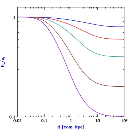
Figure 1: Ionization correlations. We show the joint probability $F_{>}$ that two points separated by a distance $d$ are in ionized regions, divided by the mean ionized fraction $x_{i}$. We consider $x_{i}=0.1$, 0.2, 0.4, 0.6 and 0.8 (bottom to top), assuming parameters for which the universe fully reionizes at $z=6.5$ due to stars in halos with efficient atomic cooling.

Our solution also allows us to calculate density-ionization correlations. Figure 2 shows the probability distribution of the density fluctuation on the scale $S_{\rm min}$ around a point $A$. In this subsection and the next, we use the notation

$$\delta_{1}(z_{1})\equiv D(z_{1})\delta_{1}\ ,$$ (46)

where the growth factor converts from the linearly-extrapolated $\delta_{1}$ at redshift 0 (which we have been using) to the linearly-extrapolated $\delta_{1}$ at redshift $z_{1}$. Given that point $A$ is neutral, we calculate as detailed in § 4.6 the separate probability distributions of $\delta_{1}(z_{1})$ given that a point $B$ a distance $d$ away is either ionized or neutral. When $d=1$ com Mpc the two points are highly correlated, and point $B$ is most likely to be neutral as well, especially when $\delta_{1}(z_{1})$ is very negative. However, when $d=10$ com Mpc the correlations are weaker, and point $B$ is most likely ionized, but only with a $65\%$ chance although the IGM as a whole is $80\%$ ionized in the plotted example.

Figure 2: Density-ionization correlations. We show in each panel the normalized probability distribution of the density fluctuation $\delta_{1}(z_{1})$ on the scale of 0.09 com Mpc (corresponding to $S_{\rm min}=46$) around a point $A$, in general (dotted curve) or given that point $A$ is in a neutral region (solid curve). For the latter, we also show the break-down into a contribution from the case where point $B$ is ionized (short-dashed curve) or where point $B$ is neutral (long-dashed curve). With the same assumptions as in Figure 1, we consider $x_{i}=0.8$ (which implies $z=7.3$) and a separation $d=1$ com Mpc (top panel) or 10 com Mpc (bottom panel).

5.2 The 21-cm Power Spectrum

During cosmic reionization, we assume that there are sufficient radiation backgrounds of X-rays and of Ly$\alpha$ photons so that the cosmic gas has been heated to well above the cosmic microwave background (CMB) temperature and the 21-cm level occupations have come into equilibrium with the gas temperature. In this case, the observed 21-cm brightness temperature relative to the CMB is independent of the spin temperature and, for our assumed cosmological parameters, is given by (Madau et al., 1997)

$$T_{b}=\tilde{T}_{b}\Psi;\ \ \ \ \tilde{T}_{b}=25\sqrt{\frac{1+z}{8}}\,{\rm mK}\ ,$$ (47)

with $\Psi=x_{\rm HI}[1+\delta(z)]$, where $x_{\rm HI}$ is the neutral hydrogen fraction and we also used the notation of eq. (46). Under these conditions, the 21-cm fluctuations are thus determined by fluctuations in $\Psi$. To determine its statistical properties using our model, we note that for a given random walk, the value of the neutral hydrogen is either 1 (if the barrier has not been pierced) or 0 (if it has).

Consider points $A$ and $B$ at a distance $d$ from each other. Then the correlation function of $\Psi$ is $\xi_{\Psi\Psi}=\langle\Psi_{1}\Psi_{2}\rangle-\langle\Psi_{1}\rangle\langle\Psi_{2}\rangle$, where the mean value is, e.g., for point 1:

$$\langle\Psi_{1}\rangle=F_{\rm<,lin}(\nu_{1},\mu_{1},S_{1})+D(z_{1})\,\bar{\delta}_{\rm lin}(\nu_{1},\mu_{1},S_{1})\ ,$$ (48)

where we set $S_{1}=S_{\rm min}$ and use eq. (17). This result arises from the fact that the average value of $\Psi$ is simple the value of $[1+\delta(z)]$ averaged only within neutral regions (where $x_{\rm HI}=1$, corresponding to random walks that have not been absorbed); e.g., the first term (unity) yields simply the fraction of the universe which is still neutral.

To average over the value of $[1+\delta_{1}(z_{1})]\times[1+\delta_{2}(z_{2})]$ when both points are neutral, we follow the derivation of eq. (39), writing, e.g., $(1+D(z_{1})\,\delta_{1})=(1+D(z_{1})\,\delta)+D(z_{1})\,(\delta_{1}-\delta)$. Note that our solution for $Q$ describes exactly those random walks that correspond to both points being neutral (i.e., not absorbed by the barrier). We obtain

$$\langle\Psi_{1}\Psi_{2}\rangle=\int_{\delta=-\infty}^{\nu_{\rm m}+\mu_{\rm m}\xi}d\delta\ Q_{\rm lin}(\nu_{\rm m},\mu_{\rm m},\delta,\xi)$$ (49)

$$\ \ \ \ \ \ \ \mbox{}\times\Bigl{[}(1+D(z_{1})\,\delta)F_{\rm<,lin}(\nu_{1}+\mu_{1}\xi-\delta,\mu_{1},S_{1}-\xi)$$

$$\ \ \ \ \ \ \ \ \ \ \ \ \mbox{}+D(z_{1})\,\bar{\delta}_{\rm lin}(\nu_{1}+\mu_{1}\xi-\delta,\mu_{1},S_{1}-\xi)\Bigl{]}$$

$$\ \ \ \ \ \ \ \mbox{}\times\Bigl{[}(1+D(z_{2})\,\delta)F_{\rm<,lin}(\nu_{2}+\mu_{2}\xi-\delta,\mu_{2},S_{2}-\xi)$$

$$\ \ \ \ \ \ \ \ \ \ \ \ \mbox{}+D(z_{2})\,\bar{\delta}_{\rm lin}(\nu_{2}+\mu_{2}\xi-\delta,\mu_{2},S_{2}-\xi)\Bigl{]}\ .$$

We use this equation with $S_{1}=S_{2}=S_{\rm min}$. However, we can calculate the correlation function of $\Psi$ down to smaller scales by assuming that the smaller-scale power does not influence the ionization and is independent of the larger scales. Thus, we simply add to $\xi_{\Psi\Psi}$ the contribution $D(z_{1})D(z_{2})[\xi_{r}(d,0,0)-\xi_{r}(d,r_{\rm min},r_{\rm min})]$ times the probability that both points are neutral, where $r_{\rm min}$ is the scale corresponding to $S_{\rm min}$. Note, though, that these scales are quite small and we expect large non-linear corrections to the model over this range of scales.

Having calculated the correlation function of the 21-cm brightness temperature, we Fourier transform it and obtain the power spectrum $P(k)$ as a function of wavenumber $k$. We express the result in terms of a characteristic quantity that has units of temperature:

$$\Delta_{21}(k)\equiv\tilde{T}_{b}\,\sqrt{k^{3}P(k)/(2\pi^{2})}\ .$$ (50)

Figure 3 shows that the 21-cm power spectrum changes shape during reionization, acquiring large-scale power and flattening on scales up to several tens of Mpc as the characteristic bubble size grows towards the end of reionization. The amount of large-scale power depends strongly on the bias of the typical ionizing galaxies. The bias is larger for more massive halos, leading to stronger large-scale fluctuations in this case. These trends are qualitatively similar to those seen in previous approximate models that were constructed more artificially [e.g., Furlanetto et al. (2006)].

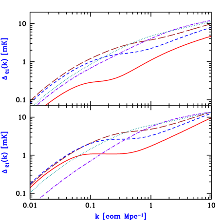
Figure 3: 21-cm power spectrum. Assuming parameters for which the universe fully reionizes at $z=6.5$, we show in each panel results for $x_{i}=0.1$ (dot-dashed curve), 0.3 (dotted curve), 0.5 (long-dashed curve), 0.7 (short-dashed curve) and 0.9 (solid curve). We consider stars forming in all halos above $V_{c}=16.5$ km/s (top panel; corresponds to efficient atomic cooling) or only in halos ten times as massive, above $V_{c}=35.5$ km/s (bottom panel; corresponds to strong feedback in low-mass halos, e.g., due to photoheating or supernovae).

As a final example, in Figure 4 we compare our model quantitatively to a numerical N-body plus radiative transfer simulation by Zahn et al. (2006). In this comparison we modify the model slightly in accordance with the assumptions in their simulation. Unlike Furlanetto et al. (2004), who effectively assumed that the star formation rate in halos is proportional to the rate of gas infall into them, Zahn et al. (2006) assumed a constant mass-to-light ratio, which sets the star formation rate in halos to be proportional to their total gas content at a given time. This assumption leads to a slightly different condition for having enough sources to ionize a given region [see Zahn et al. (2006)], which we again approximate as a linear barrier constraint. We set the minimum halo mass to be $2\times 10^{9}M_{\odot}$, as assumed in the simulation, and set the effective efficiency factor at each redshift so that the model yields the same global ionized fraction as measured in the simulation. We also compare our results to the numerical extended Press-Schechter model from Zahn et al. (2006), where they numerically applied the spherical ionization condition (in real space) to the linear density field.

These comparisons are an ambitious challenge for our model since it is fully analytical and makes necessary approximations in using spherical averages in the statistics, in applying simplifying assumptions that are strictly valid only in $k$-space, and in neglecting significant non-linear corrections. The model also relies on the two-step approximation, approximates the reionization condition as a linear barrier, and is based on a Lagrangian approach. The simulation is limited as well, with fluctuations in the measured $\Delta_{21}(k)$ indicating a lack of convergence on large scales, while on small scales the mass resolution corresponds to only 64 particles per $2\times 10^{9}M_{\odot}$ halo, well below the 500 required for reasonable confidence as indicated by careful convergence tests (Springel & Hernquist, 2003). Nevertheless, the comparison indicates that the simple analytical model captures the correct trends such as the change in power-spectrum shape with redshift, and can therefore be used to estimate the quantitative results and to explore the dependence on model parameters such as the astrophysical properties of the ionizing sources.

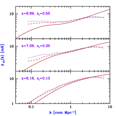
Figure 4: 21-cm power spectrum. We compare our model prediction (solid curves) to those from the simulation (dashed curves) and numerical extended Press-Schechter (dotted curves) from Zahn et al. (2006). The results are shown at several different redshifts, as indicated in each panel. At each redshift $z$ we adjust the value of the efficiency in our model in order to match the mean global ionized fraction $x_{i}$ from the simulation.

6 Summary

We have presented an approximate but fairly accurate analytical solution to the mathematical problem of the joint evolution of two correlated random walks with linear absorbing barriers. Our self-consistent solution is a generalization of the constant-barrier solution of Scannapieco & Barkana (2002) and is based on their two-step approximation. Physically this mathematical setup can be applied to a number of topics in galaxy formation where spatially-dependent feedback or two-point correlations are important.

We have emphasized in particular the direct relevance to extended Press-Schechter models of the ionizing bubble distribution during cosmic reionization (Furlanetto et al., 2004). In this context, the joint probability distribution $Q$ of the random-walk trajectories [eq. (36)] corresponds to the bivariate density distribution at two points when both points are neutral. The bivariate cumulative probability $F_{>}$ of both points hitting their barriers [eq. (40)] corresponds to the probability that both points are in ionized regions. Other distributions [e.g., as given by eq. (43)] correspond to various elements of the joint correlations among the densities and ionization states of the two points.

We have shown that our model can be used not only to calculate density-ionization correlations (Figures 1 and 2), but also (Figure 3) the power spectrum of fluctuations in the 21-cm temperature brightness, which may be observed in the next few years. Like any analytical approach to complicated non-linear physics, our model is approximate and simplified in a number of ways, but it correctly captures the trends seen in simulations of reionization (Figure 4) and thus can be used to explore various scenarios of cosmic reionization and their observable consequences.

References

- Barkana & Loeb (2002) Barkana R., Loeb A., 2002, ApJ, 578, 1
- Barkana & Loeb (2004) ——————————–, 2004, ApJ, 609, 474
- Bond et al. (1991) Bond J. R., Cole S., Efstathiou G., Kaiser N., 1991, ApJ, 379, 440
- Bowman, Morales, & Hewitt (2006) Bowman J. D., Morales M. F., Hewitt J. N., 2006, ApJ, 638, 20
- Chandrasekhar (1943) Chandrasekhar S., 1943, Reviews of Modern Physics, 15, 1
- Cole & Kaiser (1989) Cole S., Kaiser N., 1989, MNRAS, 237, 1127
- Furlanetto et al. (2006) Furlanetto S. R., McQuinn M., Hernquist L., 2006, MNRAS, 365, 115
- Furlanetto et al. (2004) Furlanetto S. R., Zaldarriaga M., Hernquist L., 2004, ApJ, 613, 1
- Iliev et al. (2005) Iliev I. T., Scannapieco E., Shapiro P. R., 2005, ApJ, 624, 491
- Kaiser (1984) Kaiser N., 1984, ApJ, 284, L9
- Lacey & Cole (1993) Lacey C., Cole S. 1993, MNRAS, 262, 627
- Madau et al. (1997) Madau, P., Meiksin, A., & Rees, M. J. 1997, ApJ, 475, 429
- McQuinn et al. (2005) McQuinn M., Furlanetto S. R., Hernquist L., Zahn O., Zaldarriaga M., 2005, ApJ, 630, 643
- McQuinn et al. (2006) McQuinn M., Zahn O., Zaldarriaga M., Hernquist L., Furlanetto S. R., 2006, ApJ, 653, 815
- Mo & White (1996) Mo H. J., White S. D. M., 1996, MNRAS, 282, 347
- Peebles (1980) Peebles P. J. E., 1980, The Large-Scale Structure of the Universe (Princeton: Princeton University Press)
- Porciani & Madau (2005) Porciani C., Madau P., 2005, ApJL, 625, L43
- Porciani et al. (1998) Porciani C., Matarrese S., Lucchin F., Catelan P., 1998, MNRAS, 298, 1097
- Press & Schechter (1974) Press W. H., Schechter P., 1974, ApJ, 187, 425