Black–body components in Gamma–Ray Bursts spectra?

Abstract

We study 7 Gamma Ray Bursts (GRBs), detected both by the BATSE instrument, on–board the Compton Gamma Ray Observatory, and by the Wide Field Camera (WFC), on board $Beppo$SAX. These bursts have measured spectroscopic redshifts and are a sizeable fraction of the bursts defining the correlation between the peak energy $E_{\rm peak}$ (i.e. the peak of the $\nu F_{\nu}$ spectrum) and the total prompt isotropic energy $E_{\rm iso}$ (so called “Amati” relation). Recent theoretical interpretations of this correlation assume that black–body emission dominates the time resolved spectra of GRBs, even if, in the time integrated spectrum, its presence may be hidden by the change of its temperature and by the dilution of a possible non–thermal power law component. We perform a time resolved spectral analysis, and show that the sum of a power–law and a black–body gives acceptable fits to the time dependent spectra within the BATSE energy range but overpredicts the flux in the WFC X–ray range. Moreover, a fit with a cutoff power–law plus a black–body is consistent with the WFC data but the black–body component contributes a negligible fraction of the total flux. On the contrary, we find that fitting the spectra with a Band model or a simple cutoff power–law model yields an X–ray flux and spectral slope which well matches the WFC spectra.

1 Introduction

Our knowledge of the spectral properties of the prompt emission of long Gamma Ray Bursts (GRBs) is based on systematic studies of their time integrated spectrum (e.g. Golenetskii et al., 1983; Band et al. 1993; Barraud et al. 2003; Amati et al. 2002) which turned out to be described by two smoothly joint power–laws with typical photon indices $\alpha\simeq-1$ and $\beta\simeq-2.5$ for the low and high energy components, respectively, or a cutoff power–law. Several studies aiming to characterise the time dependent behaviour of the spectrum (Ford et al. 1995; Preece et al. 1997; Crider et al. 1997; Ghirlanda, Celotti & Ghisellini 2002, Ryde et al. 2000; Kaneko et al. 2006) have demonstrated that the overall spectral shape and the peak energy $E_{\rm peak}$ (in a $\nu F(\nu)$ plot) evolve in time. The evolution is rather complex and there is no unique trend, but a prevalence of a hard–to–soft behaviour is observed.

The time integrated properties, however, are the one used to calculate the bolometric emitted energy of GRBs (both isotropic, $E_{\rm iso}$, and collimation corrected, $E_{\gamma}$) and to relate them to the peak energy $E_{\rm peak}$ (the so called “Amati”, “Ghirlanda” and “Liang & Zhang” relations – Amati et al. 2002; Ghirlanda, Ghisellini & Lazzati 2004, hereafter GGL04; Ghirlanda et al. 2007; Liang & Zhang 2005). Furthermore, even the correlation between the isotropic peak luminosity $L_{\rm peak}$ and $E_{\rm peak}$ (the so–called “Yonetoku” relation – Yonetoku et al. 2004), and the $L_{\rm peak}$–$E_{\rm peak}$–$T_{0.45}$ relation (the so–called “Firmani” relation – Firmani et al. 2006) make use of the time integrated spectrum (see Ghirlanda et al. 2005). The fact that these correlations apply to the time integrated spectrum, even if it evolves in time, may underline some global property of the burst.

In this respect there have been, very recently, important suggestions and new ideas for explaining the “Amati”, the “Ghirlanda” and also the “Firmani” relation. The simplest way to have a relation between the emitted energy or luminosity and $E_{\rm peak}$ is through black–body emission. Indeed, in this case, the number of free parameters is kept to a minimum: the rest frame bolometric and isotropic black–body luminosity would depend on the emitting surface, the temperature and the bulk Lorentz factor. Any other emission process would depend on some extra parameters, such as the magnetic field and/or the particle density, and it would then be more difficult, if these quantities vary from burst to burst, to produce a correlation with a relatively small scatter such as the $E_{\rm peak}-E_{\gamma}$ one.

Rees & Mészáros (2005), Thompson (2006) and Thompson, Mészáros & Rees (2006) explain these correlations assuming that a considerable fraction of the prompt emission flux is due to a black–body. This does not imply, however, that the entire observed flux is a single black–body (we already know that this is not the case).

Indeed, time integrated GRB spectra are typically described by the Band model or cutoff–power law model. The time integrated spectrum, however, being the result of the spectral evolution, could be best fitted by a model which is not the same used for the time resolved spectra. Within the black–body interpretation, there could be at least two alternatives: the time integrated spectrum (which looks like a cutoff–power law or a Band model) is (a) the result of the superposition of different black–bodies with a time dependent temperature and flux or (b) the sum of two components, i.e. one thermal (black–body) and one non–thermal (power law or double power law) as suggested by Ryde 2004. In both cases, since the temperature of the single (time resolved) black–bodies and/or the slope of the power–law can evolve in time, the time–integrated spectrum could well be modelled by a smoothly broken power–law (i.e. the Band function, see below), hiding the presence of the black–body. This requires to perform the time resolved spectral analysis in order to assess the presence of an evolving black–body component possibly with a non–thermal power–law component.

Evidences of the presence of a thermal black–body component were discovered in the BATSE spectra (e.g. Ghirlanda, Celotti, Ghisellini 2003, hereafter GCG03). This component dominates the initial emission phase up to $\sim 2$ s after the trigger. During this phase the luminosity and the temperature evolve similarly in different GRBs while the late time spectrum is dominated by a non thermal component (e.g. it is fitted with the empirical Band et al. 1993 model). Attempts to deconvolve these spectra with a mixed model, i.e. a black–body plus a power–law (Ryde et al. 2005), showed that the black–body (albeit with a monotonically decreasing flux) could be present also during later phases of the prompt emission (see also Bosnjak et al. 2005).

As a test of the recently proposed “black–body” interpretations of the $E_{\rm peak}-E_{\rm iso}$ and $E_{\rm peak}-E_{\gamma}$ correlations, we consider, among the sample of GRBs used to define these correlations, those bursts that were detected by BATSE and with published WFC spectra. Given the relatively large brightness of these bursts, it is possible for them to meaningfully analyse the time dependent properties of their spectra.

The focus of this paper is not much on the study of the spectral evolution of these few bursts, but, instead, on the relevance of the black–body in the time resolved spectra together with the relevance of the sum of the black–bodies, possibly at different temperatures, in the time integrated spectrum. To this aim we adopt for our analysis a power–law+black–body model, besides the “standard” Band and cutoff power–law model. We anticipate that the power–law+black–body model, although giving acceptable fits, is inconsistent with the WFC data. A more complex fit, made by adopting the sum of a black–body and a cutoff power–law, is equally acceptable and consistent with the WFC data, but implies that the black–body flux is a minor fraction of the total.

The paper is organised as follows: in §2 we recall the basic ideas of the “black–body” interpretation of the $E_{\rm peak}-E_{\rm iso}$ and $E_{\rm peak}-E_{\gamma}$ correlations; in §3 we introduce the sample and the spectral analysis procedure; in §3 we present the results of the time resolved spectral analysis and the comparison of the BATSE and WFC spectra with the three adopted model. We discuss our results in §4.

2 The interpretation of the spectral–energy correlations

The recent theoretical attempts to explain the spectral–energy relations, and in particular the $E_{\rm peak}-E_{\rm iso}$ (Amati) one, largely motivate the present work. Therefore it may be useful to summarise here the arguments put forward by Thompson (2006) and by Thompson, Mészáros & Rees (2006).

Consider a fireball that at some distance $R_{0}$ from the central engine is moving relativistically with bulk Lorentz factor $\Gamma_{0}$. As an example, one can think that $R_{0}$ is the radius of the progenitor star. Assume that a large fraction of the energy that the fireball dissipates at $R_{0}$ is thermalized and forms a black–body of luminosity:

$$L_{\rm BB,iso}\,=\,\pi R_{0}^{2}\Gamma_{0}^{2}\sigma{T^{\prime}_{0}}^{4}\,=\,\pi{R_{0}^{2}\over\Gamma_{0}^{2}}\sigma T_{0}^{4}$$ (1)

where $T^{\prime}_{0}$ and $T_{0}=\Gamma_{0}T^{\prime}_{0}$ are the temperatures at $R_{0}$ in the comoving and observing frame, respectively. The collimation corrected luminosity is $L_{\rm BB}=(1-\cos\theta_{\rm j})L_{\rm BB,iso}$, which, for small semiaperture angles of the jetted fireball (assumed to be conical) gives

$$\theta_{\rm j}^{2}\,\sim\,{2L_{\rm BB}\over L_{\rm BB,iso}}$$ (2)

Now Thompson (2006) and Thompson, Mészáros  & Rees (2006) introduce one key assumption: for causality reasons $\Gamma_{0}\sim 1/\theta_{\rm j}$. This allows to substitute $\Gamma_{0}$ in Eq. (1) to obtain:

$$L_{\rm BB,iso}\,\sim\,2\pi R_{0}^{2}{L_{\rm BB}\over L_{\rm BB,iso}}\sigma{T_{0}}^{4}$$ (3)

Setting $E_{\rm BB,iso}=L_{\rm BB,iso}t_{\rm burst}$ and $E_{\rm BB}=L_{\rm BB}t_{\rm burst}$, where $t_{\rm burst}$ is the duration of the prompt emission, one has

$$E_{\rm peak}\,\propto\,T_{0}\,\propto\,E_{\rm BB,iso}^{1/2}E_{\rm BB}^{-1/4}t_{\rm burst}^{-1/4}$$ (4)

This reproduces the “Amati” relation if $E_{\rm BB}$ is nearly the same in different bursts and if the dispersion of the GRB duration is not large. One can see that a key assumption for this derivation is the black–body law. It is the $L\propto T^{4}$ relation which allows to derive $E_{\rm peak}\propto E_{\rm iso}^{1/2}$.

3 Sample selection and analysis

We consider all bursts detected by BATSE with measured spectroscopic redshift which were also detected by BeppoSAX and for which the WFC data were published (Amati et al. 2002; Frontera, Amati & Costa 2000). In Tab. 1 we list our bursts and their time integrated spectral properties as found in the literature. We also report the duration ($T_{90}$) derived from the BATSE $\gamma$–ray light curve, the 50–300 keV energy fluence and the hard X–ray (2–28 keV) energy fluence. We include in our sample also GRB 980329 and 980326 for which only a range of possible redshifts (the most accurate for 980326) were found (see also GGL04).

GRB	$z$	$\alpha$	$\beta$	$E_{\rm peak}$	REF	$T_{90}$	$F$(50–300keV)	$F$(2–28keV)
				keV		s	erg cm-2	erg cm-2
970508	0.835	$-$1.71 (0.1)	$-$2.2 (0.25)	79 (23)	1, 8
	0.835	$-$1.19	$-$1.83	$>1800$	1, 9	23.1$\pm$3.8	1.1$\times 10^{-6}$	8.3$\times 10^{-7}$
971214	3.418	$-$0.76 (0.1)	$-$2.7 (1.1)	155 (30)	2, 8	31.23$\pm$1.18	6.44$\times 10^{-6}$	3.2$\times 10^{-7}$
980326	0.9–1.1	$-$1.23 (0.21)	$-$2.48 (0.31)	33.8 (17)	3, 8	…	…	5.5$\times 10^{-7}$
980329	2–3.9	$-$0.64 (0.14)	$-$2.2 (0.8)	233.7 (37.5)	4, 8	18.56$\pm$0.26	3.2$\times 10^{-5}$	4.3$\times 10^{-6}$
980425	0.0085	$-$1.26		120	5, 9	34.88$\pm$3.78	2.47$\times 10^{-6}$	1.8$\times 10^{-6}$
990123	1.6	$-$0.89 (0.08)	$-$2.45 (0.97)	781 (62)	6, 8	63.4$\pm$0.4	1.0 $\times 10^{-4}$	9.0$\times 10^{-6}$
990510	1.602	$-$1.23 (0.05)	$-$2.7 (0.4)	163 (16)	7, 8	68$\pm$0.2	1.1$\times 10^{-5}$	5.5$\times 10^{-6}$

Table 1: Time integrated properties of the bursts with spectroscopic redshift and detected by both BATSE and BeppoSAX and with published BeppoSAX–WFC spectra. The duration $T_{90}$ and the (50–300keV) fluence [$F$(50–300keV)] are from the on–line BATSE catalogue. The 2–28 keV fluence is reported from Tab. 1 of Amati et al. 2002 for all bursts except GRB 980425 for which we report the 2–26 keV fluence given in Pian et al. 2000. In the case of GRB 980326 we could not find these information in the publicly available archive. For GRB 970508 we report the spectral results of the BeppoSAX data (first line) and the results obtained from the BATSE data (second line). First set of references is for the redshift: 1) Metzger et al. 1997; 2) Kulkarni et al. 1998; 3) Bloom et al. 1999; 4) Lamb et al. 1999 (and references therein); 5) Galama et al. 1998; 6) Kulkarni et al. 1999; 7) Vreeswijk et al. 2001; Second set of references is for the spectral parameters: 8) Amati et al. 2002; 9) Jimenez, Band & Piran 2001.

For all the bursts we analysed the BATSE Large Area Detector (LAD) spectral data which consist of several spectra accumulated in consecutive time bins before, during and after the burst. Only for GRB 990123 we analysed the Spectroscopic Detectors (SD) data because of a gap in the LAD data sequence. The spectral analysis has been performed with the software SOAR v3.0 (Spectroscopic Oriented Analysis Routines by Ford et al. 1993), which we implemented for our purposes.

For each burst we analysed the BATSE spectrum accumulated over its total duration (which in most cases corresponds to the $T_{90}$ parameter reported in the BATSE catalogue) and the time resolved spectra distributed within this time interval. The time resolved spectra are accumulated on–board according to a minimum signal–to–noise criterion with a minimum integration time of 128 ms. As the bursts of our sample have quite large fluence (i.e. $\geq 10^{-6}$ erg cm^-2 integrated over the 50–300 keV range) in most cases we could analyse their time resolved spectra as they were accumulated by the on–board algorithm. Only the spectra at the beginning or at the end of the bursts (or during interpulses phases) were accumulated in time in order to have a larger signal. Energy rebinning (i.e. at least 30 (15) counts per bin for the LAD (SD) spectra) was systematically applied in our analysis in order to test the goodness of the fits through the $\chi^{2}$ statistics.

The adopted spectral analysis procedure is the standard forward–folding which folds the model spectrum with the detector response and, by varying the model free parameters, minimises the $\chi^{2}$ between the model and the data. This procedure requires the knowledge of the background spectrum corresponding to each analysed spectrum. In order to account for the possible time variability of the background we modelled it as a function of time. We selected two time intervals (before and after the burst) as close as possible to the burst (not contaminated by the burst itself) of typical duration $1000$ s. We fit the spectra contained in these intervals with a background model which is a polynomial function of time $B(E,t)$, and, being a spectrum, also of the energy $E$. Each energy bin of the spectra selected for the background calculation is interpolated with this polynomial function. This fit is tested for by inspecting the distribution of its $\chi^{2}$ as a function of energy. In this way we obtain the best fit time–dependent background model function $B_{best}(E,t)$ which is extrapolated to the time interval $\Delta t$ of each time resolved spectrum and subtracted to the data. This method is the same adopted in previous analysis of the BATSE data (e.g. Preece et al. 2000; Kaneko et al. 2006).

3.1 Spectral models

For the analysis of both the time resolved and the time integrated spectra we use three models which were already tested in fitting the BATSE spectral data (Preece et al. 2000; Ghirlanda et al. 2002; Ryde 2004; Kaneko 2006):

1. The Band (B) model (originally proposed by Band et al. 1993) which consists of 2 power laws joined smoothly by an exponential roll–over. Its analytical form is:

   $$N(E) = AE^{\alpha}\exp\left(-{E\over E_{0}}\right);\quad{\rm for}\ E\leq\left(\alpha-\beta\right)E_{0}$$

   $$N(E) = AE^{\beta}[(\alpha-\beta)E_{0}]^{\alpha-\beta}\exp(\beta-\alpha);$$ (5)

   $${\rm for}\;\;E\geq\left(\alpha-\beta\right)E_{0}$$

   The free parameters, which are the result of the fit to the observed spectrum, are: the normalisation of the spectrum $A$; the low energy power law photon spectral index $\alpha$; the high energy power law photon spectral index $\beta$ and the break energy, which represents the e–folding parameter, $E_{0}$. If $\beta<-2$ and $\alpha>-2$ this model has a peak in the $EF_{E}$ representation which is $E_{\rm peak}=(\alpha+2)E_{0}$. In the fits we assume that $\alpha$ and $\beta$ can vary within the range [$-5$, 1] while the break energy is allowed to vary in the same range covered by the spectral data, i.e. $\sim$ 30–1800 keV. The B model is a fair representation of the spectral model produced in the case of emission from a relativistic population of electrons, distributed in energy as a single or a broken power law, emitting synchrotron and/or inverse Compton radiation, and can also reproduce the case of an electron energy distribution which is a Maxwellian at low energies and a power law at high energies, emitting synchrotron radiation (e.g. Tavani et al. 1996).

2. The cut–off power law (CPL) is composed by a power law ending–up in an exponential cutoff. It corresponds to the previous Band model without the high energy power–law component. Its form is:

   $$N(E)=AE^{\alpha}\exp\left(-\frac{E}{E_{0}}\right)$$ (6)

   The free parameters are the same of the Band model without the high energy component. If $\alpha>-2$ also this model presents a peak in its $EF_{E}$ representation which is $E_{\rm peak}=(\alpha+2)E_{0}$. This model can represent the case of thermal or quasi–thermal Comptonization, even when saturated (i.e. a Wien spectrum, with $\alpha=2$).

3. The black–body + power–law (BBPL) model is

   $$N(E)=A\frac{E^{2}}{\exp(E/kT)-1}+BE^{\alpha}$$ (7)

   where $\alpha$ is the spectral index of the power–law; $kT$ the black–body temperature and $A$ and $B$ are the normalisations of the two spectral components. In this case, the peak of the $\nu F_{\nu}$ spectrum depends on the relative strength of the two model components and on the spectral energy range where the spectrum is considered. The peak energy of the black–body component only is $E_{\rm peak,BB}=3.93kT$ (in $\nu F_{\nu}$). The (simplest) physical rationale of this model is the possible different origin of the two components: the thermal black–body emission could be photospheric emission from the fireball (e.g. Daigne & Mockovitch 2000) while the power–law component might be the non–thermal emission from relativistic electrons accelerated above the photosphere at the classical internal shock radius (see also Pe’er, Meszaros & Rees 2006). The BBPL model is the simplest spectral model which combines a thermal and a non–thermal component. In §5 we will also discuss the more complex case of a cutoff power–law plus a black–body component.

Note that the number of free parameters is the same (i.e. four, including normalisations) in the B and BBPL model while the CPL model has one less free parameter.

The BATSE spectra were fitted in the past with all these models. Band et al. (1993) proposed the B function to fit the time integrated spectra of bright long GRBs. Also the time resolved spectra could be fitted by either the B or the CPL model (Ford et al. 1995; Ghirlanda, Celotti & Ghisellini 2002). More recently Kaneko et al. (2006) performed a systematic analysis of the time resolved spectra of a large sample of BATSE bursts selected according to their peak flux and fluence. From these works it results that the typical low energy spectral slope (in both the B and CPL model) has a wide distribution centred around $\alpha\sim-1$ with no preference for any specific value predicted by the proposed emission models (i.e. $\alpha=-2/3$ for optically thin synchrotron – Katz et al. 1994; $\alpha=-3/2$ for synchrotron cooling – Ghisellini & Celotti 1999; $\alpha=0$ for jitter radiation – Medvedev 2000). The high energy photon spectral index $\beta$ has a similar dispersion (i.e. 0.25) of the $\alpha$ distribution and its typical value is –2.3. The peak energy has a narrow ($\sigma\leq 100$ keV) distribution centred at $\sim$ 300 keV. A small fraction (7%) of the time resolved spectra have $\beta>-2$ which means that the peak energy of the $EF_{E}$ spectrum is above the upper energy threshold (i.e. $E_{\rm peak}>2$ MeV). The composite BBPL model was fitted to the time resolved spectra of a few bright BATSE bursts (Ryde 2005, Bosnjak et al. 2005).

In the following section we present the spectral parameters of the fits obtained with the three models above. The scope of this paper is not to decide which (if any) of the proposed models best fits the spectra. It has been already shown (e.g. Ryde 2005) that the time resolved BATSE spectra can be adequately fitted with both the B(CPL) model and the BBPL model.

4 Results

We here show the spectral evolution and compare the spectral parameters of the three models described in §3. We also compare the spectral results of our analysis of the BATSE time integrated spectra (reported in Tab. 2) with the results gathered from the literature (Tab. 1). We then discuss the contribution of the black–body component to the spectrum and compare the spectral fits of the three models with the constraints given by the WFC data.

4.1 Spectral evolution

We present the spectral evolution of the fit parameters obtained with the three models described in §3.

4.1.1 GRB 970508

The spectral parameters of the time integrated spectrum published in Amati et al. (2002) for GRB 970508 were found by the analysis of the WFC [2–28 keV] and Gamma Ray Burst Monitor [GRBM, 40–700 keV] data and they differ from those found by the BATSE spectral analysis and published in Jimenez et al. (2000). We report the different results in Tab. 1. The main difference is that according to the BeppoSAX spectrum this burst has a considerably low peak energy while the BATSE spectrum indicates that $E_{\rm peak}>$1800 keV. We have re–analysed the BATSE spectrum confirming the results found by Jimenez et al. (2000). In particular we found an unconstrained peak energy when fitting both the B and CPL model. The spectrum in the 40–700 keV energy range of GRB 970508 presented in Amati et al. (2002) is composed by only two data points with a quite large associated uncertainty. In this case the fit (with the B model) is dominated by the WFC spectrum, which does not present any evidence of a peak (in $\nu F_{\nu}$) within its energy range. Combining the GRBM and WFC data Amati et al. (2002) found $E_{\rm peak}=79$ keV, but the GRBM spectral data appear consistent also with an high energy component with $\beta\geq-2$ (which is what is found from the fit of the BATSE spectrum). If the real GRB spectrum is that observed by BATSE this burst would be an outlier for the Amati correlation (see also Fig. 3 of GGL04). Given the possible uncertainties of the BeppoSAX spectrum, we do not consider this burst in the following analysis because the BATSE spectrum does not allow to constrain its peak energy.

4.1.2 GRB 971214

Figure 1: Spectral evolution of GRB 971214. Top panels: Band model fit results. The first panel represents the light curve (in counts/s detected at energies $\geq$ 25 keV – without the background subtraction). Mid panels: cutoff power–law fit results. Bottom panels: black–body+power–law fit results (we also report the contribution of the black–body component to the total flux in the observed 30 keV–2 MeV energy range). For all the three models we show for comparison the optically thin synchrotron limit ($\alpha=-2/3$, dashed lines) and the case of synchrotron cooling ($\alpha=-3/2$, dot dashed line).

Figure 2: Spectral evolution of GRB 980329. Symbols are the same of Fig.1.

Figure 3: Spectral evolution of GRB 980425. Symbols are the same of Fig.1.

GRB 971214 (BATSE trigger 6533) has a highly variable light curve (Fig. 1 – top panels) and the time resolved spectral analysis could be performed on $\sim$ 20 s of the total GRB duration. In this time interval we extracted 13 spectra. In Fig. 1 we show the time evolution of the spectral parameters for the B, CPL and BBPL model

The low energy spectral index $\alpha$ of the B and CPL model evolves similarly, and for most spectra this parameter violates the optically thin synchrotron limit (i.e. $\alpha=-2/3$; dashed line in Fig. 1) and, of course, the optically thin synchrotron limit in the case of radiative cooling (i.e. $\alpha=-3/2$; dot–dashed line in Fig. 1). In the case of the BBPL model instead $\alpha$ is always consistent with (i.e. softer than) these limits and softer than the corresponding values found with the B or CPL model. The peak energy of the three models is very similar and tracks the light curve although it does not change dramatically. The BBPL fit shows that the peak energy of the black–body component tracks the light curve. The black–body can contribute up to $\sim$50% of the total flux.

All three models give acceptable fits for the time integrated spectrum, accumulated over 20 s. The B model high energy component is very soft (i.e. $\beta\sim 5$) making it consistent with the CPL model. For both these two models $\alpha\sim-0.66\pm 0.08$ (1$\sigma$ uncertainty, see Tab. 2), consistent with the value reported in Tab. 1 that was derived by fitting the WFC+GRBM BeppoSAX data (Amati et al. 2002).

4.1.3 GRB 980326

For GRB 980326 (BATSE trigger 6660) both the duration and the light curve are not available in the BATSE archive. By analysing the spectral evolution we could extract only two spectra in approximately the total duration of the burst ($\sim$5 sec). The first spectrum (from 0.09 to 1.56 s) is well fitted by the B and CPL models which give similar results, i.e. $\alpha=1.2\pm 0.3$, $\beta_{B}=-3.4\pm 0.7$ and $E_{\rm peak}=52\pm 27$ keV, with $\chi^{2}_{r}=0.93$ (for 102 degrees of freedom) and $\chi^{2}_{r}=0.94$ (for 103 degrees of freedom) for the B and the CPL model, respectively. The second spectrum (from 1.56 to 4.09 s) has $\alpha$ and $E_{\rm peak}$ consistent with the first one. These two spectra, fitted with the BBPL model show a soft power–law component (i.e. $\alpha_{BBPL}\sim-2.5$) and peak energy of $\sim$ 74 keV (with $\chi^{2}_{r}=1.0$).

The spectral parameters of the average spectrum of GRB 980326 are reported in Tab. 2 and they are consistent with those reported in Tab. 1. The only difference is the sligthly larger value of $E_{\rm peak,B}\sim 65$ keV (with $\chi^{2}_{r}=1.02$) obtained here.

4.1.4 GRB 980329

GRB 980329 (BATSE trigger 6665) has a structured light curve (Fig. 2 top panels) with at least two small peaks preceding two major peaks of similar intensity. For the spectral evolution we could accumulate 37 time resolved spectra within the $\sim$17 s duration of the burst corresponding to its $T_{90}$.

The low energy spectral index $\alpha$ evolves similarly in the B and CPL model and its values are between the two synchrotron limits (i.e. –2/3 and –3/2). The fit with the BBPL model instead requires a very soft power–law component and a time evolution similar to that of the power–law index of both the B and CPL model, but with a value which is always smaller than –3/2.

The peak energy seems to evolve differently in the B and CPL model. In the B model $E_{\rm peak}$ does not change much during the burst and remains below $\sim$ 300 keV, whereas in the CPL model $E_{\rm peak}$ changes in time and reaches $\sim$ 1 MeV in correspondence of the major peak of the light curve (at 6 s). The fit with the BBPL model instead presents a peak energy which does not evolve much and, similarly to the B fit, stays constant at around 200 keV. The black–body component contributes, at least, 40% of the total flux (bottom panel in Fig. 2).

The average spectrum of GRB 980329 has been accumulated over its $T_{90}$ and fitted with the three models. We found $\alpha=-0.93\pm 0.1$, $\beta=-2.4\pm 0.2$ and $E_{\rm peak}=253\pm 10$ keV (Tab. 2) for the fit with the B model. These spectral parameters are in good agreement (except for a softer low energy spectral index) with those found by the fitting of the BeppoSAX data by combining the WFC/GRBM data (Amati et al. 2002) reported in Tab. 1. We note that a few time resolved spectra of this burst and also the time integrated spectrum have a quite large $\chi^{2}_{r}$ when fitted with all the three models. We suspect that this is due to the fact that these spectra are characterized by very small statistical errors. Indeed, we found that the use of a 2% of systematic errors uniformly distributed in the spectral range makes the fits acceptable. However, to the best of our knowledge, this has not been treated in the published literature. For this reason we list the spectral results as they were obtained without accounting for additional systematic uncertainties. When accounting for systematic errors, the $\chi^{2}$ improves, the fitted parameters remain unchanged and their associated uncertainties slightly increase.

4.1.5 GRB 980425

GRB 980425 (BATSE trigger 6707) is a long single peaked smooth GRB famous for being the first GRB associated with a SN event (i.e. SN1998bw – Galama et al. 1998). GRB 980425 is also the lowest redshift GRB ever detected. Due to its relatively low fluence, its isotropic equivalent energy is small compared to other bursts. Indeed, it is one of the two clear outliers (the other being GRB 031203) with respect to the $E_{\rm peak}-E_{\rm iso}$ correlation (but see Ghisellini et al. 2006).

To the aim of studying its spectral evolution we extracted 7 spectra during roughly 15 s. The time interval covered by our time resolved spectral analysis is between the two durations $T_{90}$ and $T_{50}=9.79\pm 0.29$ which, however, differ by a factor 10. This limitation is due to the slow decay of the light curve after the trigger coupled to a relatively small intensity of the burst. As a result we could not constrain the spectral parameters of any spectrum during the 15–33 s time interval. However, our spectral analysis covers the main part of the single pulse of the light curve and excludes only the last decaying part of the light curve.

Although the B and CPL model can fit the time resolved spectra and give consistent results (top and mid panels of Fig. 3), we note that in 4 out of 7 spectra the B model yields an unconstrained high energy spectral index $\beta$, suggesting that the CPL model represents the data better. The low energy spectral index $\alpha$ in both cases is harder than the cooling limit, and for 3 out of 7 spectra it also violates the optically thin synchrotron limit. The evolution of the peak energy is smooth and it decreases monotonically from $\sim$ 200 keV at the beginning to few tens of keV in the final part of the burst.

The fit with a BBPL model (Fig. 3 bottom panel) gives a soft power–law index, remaining softer than $-3/2$ during the burst evolution. Overall we note that the black–body contribution to the total flux is around 40% except for one spectrum that has a quite considerable black–body flux (i.e. $\sim$80%). The peak energy (in this case the peak of the black–body component) is consistent, in terms of values and evolution, with that of the B and CPL model.

The time integrated spectrum, accumulated over the 33 s of duration of the burst, is well fitted by the three models although, also in this case, the B model has $\beta$ unconstrained. The low energy spectral index of the time integrated spectrum is $\alpha=-1.26\pm 0.14$ and the peak energy is $E_{\rm peak}=123\pm 36$ keV (Tab. 2), consistent with those reported in Tab. 1. The BBPL model fitted to the time integrated spectrum gives a very soft power–law ($\alpha=-2.19\pm 0.16$) and a peak energy of the black–body component $E_{\rm peak}\sim 137$ keV, which is consistent with the fit obtained with the CPL model.

4.1.6 GRB 990123

Figure 4: Spectral evolution of GRB 990123. Symbols are the same of Fig.1.

GRB 990123 (BATSE trigger 7343) is a long duration event with a very high fluence. The light curve has two major peaks and a long tail after the second peak. There is a gap in the LAD data corresponding to the beginning of the burst up to 20 s. For this reason we used the SD data. The spectral evolution (Fig. 4) shows that the peak energy slightly precedes the light curve first peak while it tracks the second peak (see e.g. Ghirlanda, Celotti & Ghisellini 2002). The low energy spectral component is harder than the synchrotron limit during most of the two major peaks. The B and CPL model have similar time resolved spectral parameters. The BBPL model fits the time resolved spectra with a power–law component which is harder than the $-1.5$ limit. The black–body flux is no more than 50% of the total flux.

The time integrated spectrum accumulated over $\sim$100 s (in order to include the long tail of the second peak) is fitted by both the B and the CPL model. These models give similar results: the low energy spectral index is $\alpha=-0.85\pm 0.04$ (B) and $\alpha=-0.9\pm 0.03$ (CPL); the peak energy is $E_{\rm peak}\sim 605$ keV (B) and $E_{\rm peak}\sim 684$ keV (CPL). The latter values are lower than those reported in Tab. 1. This is likely due to the better energy coverage of the BATSE data (with respect to the GRBM spectrum – Amati et al. 2002): the extension of the energy range up to 1800 keV allows to better determine the value of $E_{\rm peak}$.

4.1.7 GRB 990510

Figure 5: Spectral evolution of GRB 990510. Symbols are the same of Fig.1.

GRB 990510 (BATSE trigger 7560) has a light curve with two main structures (lasting 10 and 20 s respectively) composed by several sub–peaks and separated by a quiescent phase lasting $\approx$30 s. We could extract 6 spectra (distributed between 0 and 8 s) corresponding to the first set of peaks and 17 spectra (between 40 and 60 s) corresponding to the second set of peaks. Given the long quiescent phase we analysed separately the time average spectra integrated over the first and the second phase.

The time resolved spectra are well fitted with the CPL and the B model which give similar results (see Fig. 5). The comparison of the low energy spectral index and the peak energy between the first and the second phase shows that the spectrum of the latter is (on average) slightly softer in terms of $\alpha$ and harder in terms of $E_{\rm peak}$ than the former. The low energy spectral index $\alpha$ is harder than the optically thin synchrotron limit for most of the first peak and is consistent with this limit during the second emission episode. $E_{\rm peak}$ rises and decays during the first peaks while it has a more regular hard–to–soft evolution during the second set of peaks.

The fit with the BBPL model (Fig. 5 bottom panels) is consistent with the behaviour observed in previous bursts. In the case of the first peak we could not constrain the black–body component of the BBPL model. We therefore fixed, only for the time resolved spectra of the first peak, the black–body temperature so that its peak corresponds to the value found by fitting the B model. In the case of the BBPL model the power–law component is much softer than the low energy component of the CPL model and does not violate the $-3/2$ (cooling) limit. The peak energy of the black–body component evolves similarly to that of the CPL (or B) model and is slightly harder in the second emission phase than in the first. The black–body component contributes at most 30% of the total flux of the time resolved spectra.

The time integrated spectra of the first and second set of peaks have been fitted separately (Tab. 2). The spectral parameters of the fit of the second peak are consistent with that reported in Tab. 1 obtained with the BeppoSAX WFC+GRBM data (Amati et al. 2002).

GRB	Model	$\alpha$	$\beta$	$E_{\rm peak}$	$\chi_{r}^{2}$	$\alpha_{PL}$	% $F_{BB}$	% $F_{BB}^{BBCPL}$
971214	CPL	$-$0.65 (0.1)	….	186 (15)	1.07	$-$1.9	36	23
980326	CPL	$-$1.21 (0.44)	…	65 (35)	1.02	$-$2.7	5	$<$1
980329	Band	$-$0.93 (0.1)	$-$2.4(0.1)	253 (10)	1.6∗	$-$1.7	30	26
980425	CPL	$-$1.26 (0.14)	…	123 (36)	1.04	$-$2.1	45	8
990123	Band	$-$0.85 (0.04)	$-$2.44 (0.23)	607 (71)	1.04	$-$1.5	38	33
990510	CPL	$-$0.88(0.01)	…	92 (6)	1.3∗	$-$2.12	32	1.3
	Band	$-$1.16(0.05)	$-$2.28(0.06)	173(21)	1.5∗	$-$1.92	18	13

Table 2: Time integrated properties of the bursts of our sample. Spectral parameters were obtained from the analysis of the time integrated spectrum of the BATSE data. We report the best fit model parameters. For GRB 990510 we give the spectral results of the first and the second emission episodes separately. $*$ in these cases (see text) the reported $\chi^{2}_{r}$ (and the uncertainties associated to the spectral parameters) are without adding systematic errors to the fit (see text). $\alpha_{PL}$ represents the photon spectral index of the power–law component of the BBPL model fitted to the time integrated spectrum. $F_{BB}$ represents the average of the black–body contribution to the total flux obtained in the fits of the time resolved spectra. In the final column we show the contribution of the black–body component when fitting a more complicated model (see text) composed by a cutoff power–law plus a black–body. In these fits the black–body peak energy has been fixed to the value obtained by the fit of a simple CPL model. These results represents an upper limit to the black–body component, i.e. obtained by forcing the black–body to contribute to the peak of the spectrum. The reported black–body percentage is obtained by integrating in time the single contribution obtained by the fit of the time resolved spectra.

4.2 Inconsistency of the black–body+power law model with the Wide Field Camera data

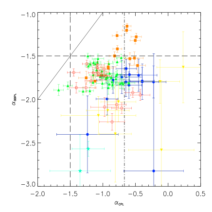
Figure 6: Comparison of the photon index of the power–law component of the BBPL model ($\alpha_{\rm BBPL}$) with the low energy photon spectral index obtained from the CPL fit ($\alpha_{\rm CPL}$). Different symbols correspond to: 971214 (filled circles), 980326 (filled stars), 980329 (triangles), 980425 (upside–down triangles), 990123 (squares) and 990510 (open circles). The solid line represents the equality of the two spectral indices. The long–dashed line and the dot–dashed line are the synchrotron limits with and without cooling, respectively.

The results obtained from the time resolved analysis of the GRBs of our sample indicate that the fit with a black–body+power–law model gives acceptable results for all bursts. This model has also the advantage, with respect to the Band and the cutoff power–law model, to require a soft power–law component with a spectral index always consistent (except for GRB 990123) with a cooling particle distribution (i.e. $\alpha<-3/2$). In Fig. 6 we compare the photon index of the CPL model (which is in most cases consistent with $\alpha$ of the B model) to that the BBPL model. Note that the latter is always softer than the corresponding parameter of the CPL model. In the same plot we also mark the synchrotron limits and show that the power–law of the BBPL model is consistent with these limits being (except for GRB 990123) softer than $-3/2$. Also when considering the time integrated spectra we find that the power–law component of the BBPL model is systematically softer than the power–law components of the B or CPL model (compare col. 7 and col. 3 in Tab. 2).

The peak energy $E_{\rm peak}$ resulting from fitting the data with the BBPL model is indeed produced by the black–body component which substantially contributes to the total energetics, at least in the observed energy range of BATSE. This would thus favour the “black–body interpretation” of the spectral–energy correlation which we have summarised in Sec. 2.

However, these results are based on the spectral analysis of the BATSE spectra only. Although covering two orders of magnitude in energy, these data do not extend below 20 keV and above 2000 keV. The low energy limit is particularly relevant here, since for these bursts we do have the information of the low (2–28 keV) energy emission from the WFC of BeppoSAX. We can then compare the result of the BBPL model with the flux and spectrum observed by the WFC. Since the latter concerns the time integrated spectrum, we should then either add the single time resolved spectra to construct the total flux and spectrum for each burst, or use the result obtained fitting the BATSE time integrated spectrum. In both cases we have to extrapolate the model to the energy range of the WFC.

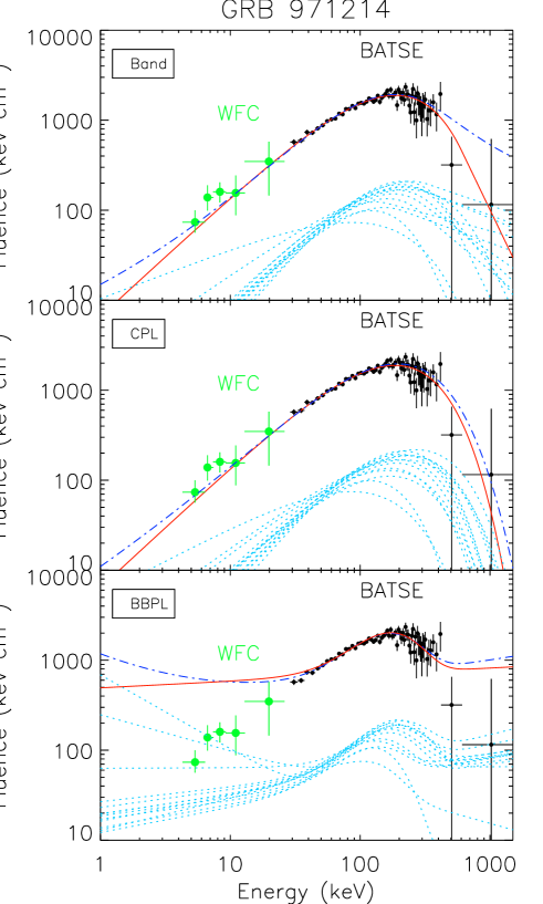
Figure 7: GRB 971214: BATSE time integrated spectrum and WFC data (black and grey points, respectively). In the three panels we show the spectral fits of the time resolved spectra (dotted lines), the spectral fit of the time integrated spectrum (solid line) and the sum of the time resolved spectral fits (dot–dashed line). Spectral fits with the B model (top panel), CPL model (mid panel) and BBPL model (bottom panel) are show.

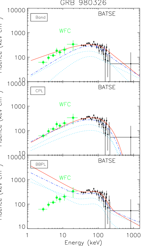
Figure 8: GRB 980326. Symbols are the same of Fig.7

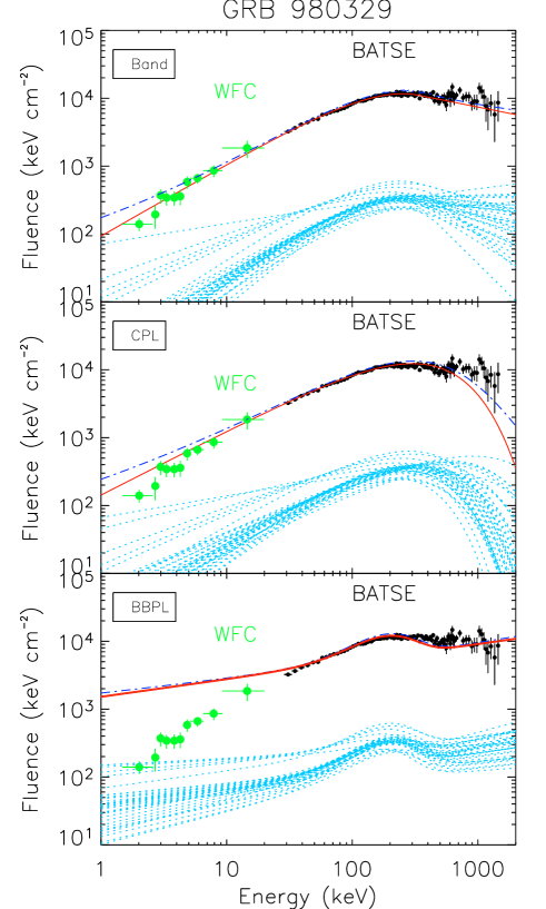
Figure 9: GRB 980329. Symbols are the same of Fig.7

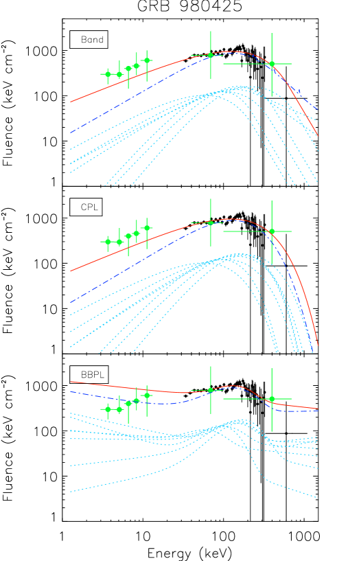
Figure 10: GRB 980425. Symbols are the same of Fig.7. In this case we also show the two data points of the GRBM instrument on board BeppoSAX covering the 40-700 keV energy range.

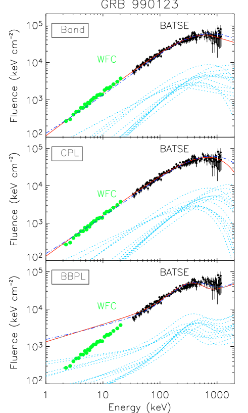
Figure 11: GRB 990123. Symbols are the same of Fig.7

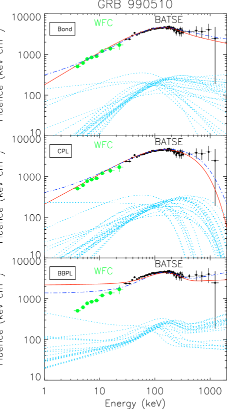
Figure 12: GRB 990510. Symbols are the same of Fig.7

As stated above, the inclusion of the black–body component implies that the accompanying power–law component becomes soft (i.e. $\alpha<-1.5$). It is this power–law component that mainly contributes at low energies, and we find, in all cases, a strong disagreement between the extrapolated flux and spectrum of the WFC data.

This is shown in Figg. 7, 8, 9, 10, 11, 12, where we report the BATSE time integrated spectrum and the WFC spectrum. In the three panels of these figures we report the results of the fit with the three models described in Sec. 3, i.e. the Band model (B), the cutoff power–law model (CPL) and the composite model (black–body plus power–law – BBPL). We report both the model fit to the time integrated spectrum (solid line) to the time resolved spectra (dotted lines) and the sum of the time resolved model fits (dot–dashed line).

One can see that in all cases the BBPL model strongly overpredicts the observed flux in the WFC 2–28 keV energy band, with a slope which is much softer than observed. This occurs both when we sum the time resolved spectra and when we use the time integrated fits. On the contrary, note the excellent agreement of the extrapolated flux and the WFC data in the case of the B and the CPL fits. To the best of our knowledge, this is the first time that a detailed comparison of the WFC $Beppo$SAX and the BATSE data is performed. We conclude that they are in excellent agreement if the spectrum is indeed described by the Band or CPL model, and that the BBPL model cannot reproduce the WFC data.

We can also conclude that a fit with a black–body only (without the power–law) is never consistent with the data, even when considering spectra at the peak of the light curve or for the first phases of the emission. This is because fitting the CPL model, which can mimic a black–body when $\alpha=1$, always gives $\alpha<0$.

Our analysis also shows that the black–body component in the time resolved spectra that we have analyzed (typically with $>$0.1 s time resolution) does not change much during the burst. This implies that even if it were possible to perform the spectral analysis with a finer temporal resolution, it is unlikely that the time resolved spectra are the superposition of a multi–temperature black–body.

Finally, we cannot exclude the possibility that the istantaneous spectrum is produced by a superposition of black–body components. Indeed, this is exactly what happens in thermal or quasi–thermal Comptonization models (if the seed photons have a relatively narrow range of frequencies), where the superposition of different scattering orders (each one being black–body like) produces the cut–off power law spectrum. Black–body components produced in different (and independent) emitting regions, instead, are less likely, since some fine tuning is required in order to produce the smooth observed spectrum.

4.2.1 Further testing the black–body component

The existence and the relevance of a black–body component in the spectra of our GRBs can be further tested allowing for the possibility that the real spectral model is more complicated than what we thought. We could make the black–body+power–law model fits consistent with the WFC [2–28 keV] spectra by introducing a spectral break between the BATSE and the WFC energy ranges. This could indeed be the case if the non–thermal component is produced by an electron energy distribution with a low energy cutoff, or if the apparently non–thermal component is instead the result of a thermal Comptonization process (e.g. Liang 1997; Liang et al. 1997; Ghisellini & Celotti 1999; Meszaros & Rees 2000). In the latter case what we see in the WFC could be the (hard) spectrum of the seed photons, while in BATSE we may see the sum of the Comptonization spectrum and a black–body.

We must then check if, in this case, it is possible that a black–body is present, is responsible for a significant fraction of the total flux and for the observed $E_{\rm peak}$, without violating any observational constraint. If so, then the “black–body” interpretation presented in §2 would receive support.

However, there are severe problems with this possibility. The first is that the required break should always be at $\sim$30 keV (between the BATSE and the WFC energy ranges) despite the fact that our GRBs have different redshifts. This makes this possibility rather ad hoc.

The second problem comes from the following test. As stated, we should use a model composed by black–body plus a Band spectrum. This model, unfortunately, has too many free parameters to yield strong constraints, but we can mimic it by adopting a model composed by the sum of a black–body and cutoff power–law. The index of the latter should be thought as the low energy index of the Band model. Furthermore, since what we really put on test is the presence of a relevant black–body, we can also fix its temperature requiring it to give the $E_{\rm peak}$ found when using the CPL (or B) model. This is because we already know that are these $E_{\rm peak}$, when combined in the time integrated spectrum, that give the $E_{\rm peak}$ used for the Amati and Ghirlanda correlations.

We thus use this black–body+cutoff power–law model (BBCPL):

$$N(E)=A\frac{E^{2}}{\exp(E/kT)-1}+BE^{\alpha}\exp\left(-\frac{E}{E_{0}}\right)$$ (8)

where $kT$, i.e the black body characteristic temperature, is fixed so that 3.9$kT$=$E_{\rm peak}$ (as found from the fit of the CPL model to each time resolved spectrum). This model has the same number of free parameters of the BBPL and B model (the two normalisations, $E_{0}$ and $\alpha$).

In Fig. 13 we compare the photon index found with a simple CPL model and the $\alpha$ of the BBCPL model described above. In the BBCPL model the photon index of the CPL component can fit the WFC data and indeed we found it to be consistent with the values found by the fit of a simple CPL model. Instead, the black–body component is negligible in all these fits.

For each time resolved spectrum fitted with the BBCPL model we can compute the fraction of the rest frame bolometric flux contributed by the black–body component. Summing up these contributions for the entire duration of each burst we derive the contribution of the black–body to the time integrated flux. The values are reported in Tab. 2 (last column): for all the bursts this contribution is small.

We can then conclude that if a black–body is present, with a temperature consistent with the peak of the spectrum (found by fitting the CPL model) then its flux is not relevant. Consider also that this spectral model is not required by the data, which are instead well described by the simpler CPL (or B) model. In this sense what we found is an upper limit to the possible contribution of a black–body to the total flux.

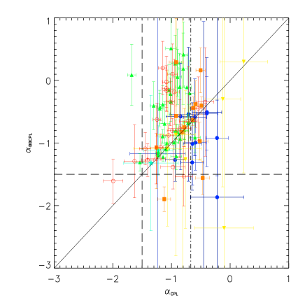
Figure 13: Comparison of the spectral photon index of the CPL model ($\alpha_{\rm CPL}$) with the photon index obtained from the fit of a cutoff power–law plus a black–body with the peak of the black–body fixed to the values found from the fit of a simple CPL model. Symbols are as in Fig. 6

5 Summary of results

We have analysed the spectra of 7 GRBs detected by BATSE with measured redshift and for which also the BeppoSAX WFC spectrum has been published (Amati et al. 2002). We analysed both the time resolved and the time integrated spectrum with three models: the Band model (B), a cutoff power–law model (CPL) and a black–body+power–law model (BBPL). For a further test of the importance of a possible black–body component we have also used the sum of a black–body plus a cutoff power–law model (BBCPL). The comparison of the spectral parameters and the analysis of the spectral evolution has shown that:

• the time resolved spectra could be reasonably fitted with all models. The spectral parameters of the B and CPL model agree within their uncertainties;

• in all our GRBs the spectral slope of the low energy component of the B or CPL model violate both the optically thin synchrotron limit with ($-1.5$) or without ($-0.67$) radiative cooling;

• the values of $\alpha<0$ found from the fit of the CPL model exclude the possibility that a single black–body model can fit these spectra (as the black–body coincides with the CPL model only for $\alpha=1$);

• the power–law slope of the BBPL model is softer than the corresponding parameter of the B or CPL model. In most GRBs (except GRB 990123) this component is softer than the optically thin synchrotron limit with cooling ($-1.5$) and softens as time goes by;

• the peak energies of the black–body component of the BBPL model found here are similar to the values found for a few other bursts analysed with the BBPL model (Ryde et al. 2005) or with a single black–body component (GCG03);

• the black–body flux (in the BBPL model) is no more than 50% of the total flux and it changes with time. In these bursts the black–body does not dominate the initial emission phase as was the case of the few GRBs analysed by GCG03;

• the soft power–law spectra found using the BBPL model implies a relatively large flux of the spectrum extrapolated at lower energies. This extrapolation is inconsistent with the WFC data and spectra (Figg. 7, 8, 9, 10, 11, 12);

• the time integrated spectral fit and the sum of the time resolved spectral fits with either the B and CPL model are consistent with the WFC spectrum both in terms of flux and slope;

• fitting the BATSE spectra with the BBCPL model results in a cutoff power–law component whose extrapolation to the WFC energy range is consistent with the observed spectrum in terms of flux and slope. In this case, however, the black–body flux is not significant.

6 Conclusions

The most important results of this work is the assessment of the importance of a black–body component in the spectra of GRBs. For the GRBs analysed here, we find that it cannot be, at the same time, responsible for the peak (in $\nu F_{\nu}$) of the spectrum and for its total energetics. We could reach this conclusion by analysing the time resolved spectra of those GRBs detected by BATSE and the by the WFC of BeppoSAX, therefore using the energy range between 2 keV and 2 MeV. We also find that the BATSE data, fitted by a cutoff power–law or by the Band model, are entirely consistent with the WFC data.

These findings bear important consequences on the interpretation of the peak–energy correlations (including the Amati, the Ghirlanda, and the Firmani correlations) put forward recently by Thompson (2006) and by Thompson, Meszaros & Rees (2007). This interpretation requires that the black–body component is responsible for the peak energy $E_{\rm peak}$ and for a significant fraction of the bolometric emitted energy. Note that, since the temperature of the black–body component may vary in time, the time integrated spectrum may not be particularly revealing of the black–body presence, making a time resolved analysis mandatory.

One may argue that the spectrum is even more complex than what we thought, having an additional break and becoming harder at low energies. Such a break is expected if the spectrum is due to a thermal photospheric emission (the black–body component) superimposed to non–thermal emission due to some dissipative mechanism (Meszaros & Rees 2000). An alternative possibility is that the observed spectra result from multiple Compton up–scattering of soft seed photons (e.g. Ghiselllini & Celotti 1999; Thompson 2005). In such a case a break is expected between the (possibly) hard seed photon spectrum and the beginning of the Comptonized spectrum.

But even by fitting the spectra with a more complex model allowing for this break, we found that the black–body component is not relevant. This, together with the rather ad hoc requirement to have a break always at 30 keV (observed) irrespective of the different redshifts of our GRBs, lead us to conclude that the presence of relevant black–body in the spectrum of our GRBs is to be excluded. This in turn, makes more problematic (and mysterious) the interpretation of the spectral–energy correlation in long GRBs.

References

- [] Amati, L., Frontera, F., Tavani, M. et al., 2002, A&A, 390, 81
- [] Band, D., Matheson, J., Ford, L., et al., 1993, ApJ, 413, 281
- [] Barraud C., Olive, J.-F., Lestrade, J.P., et al., 2003, A&A, 400, 1021
- [] Bloom J.S. Kulkarni, S.R., Djorgovski, S.G., et al., 1999, Nature, 401, 453
- [] Crider, A., Liang, E.P. & Smith, I.A., 1997, ApJ, 479, L39
- [] Firmani, C., Ghisellini, G., Avila–Reese, V. & Ghirlanda, G., 2006, MNRAS, 370, 185
- [] Ford, L.A., Band, D.L., Matteson, J.L., et al., 1995, ApJ, 439, 307
- [] Ford L., 1993, A Guide to the Spectroscopic Oriented Analysis Routines version 2.1
- [] Frontera F., Amati L. & Costa E., 2000, ApJS, 127, 59
- [] Galama, T., Vreeswijk, P.M., van Paradijs,J., et al., 1998, Nature, 395, 670
- [] Ghirlanda, G., Celotti, A. & Ghisellini, G., 2002, A&A, 393, 409
- [] Ghirlanda, G., Celotti, A. & Ghisellini, G., 2003, A&A, 406, 879 (GCG03)
- [] Ghirlanda, G., Ghisellini, G. & Lazzati, D., 2004, ApJ, 616, 331 (GGL04)
- [] Ghirlanda, G. Ghisellini, G., Firmani, C., Celotti, A. & Bosnjak, Z., 2005, MNRAS, 360, L45
- [] Ghirlanda, G., Nava, L., Ghisellini, G., et al., 2007, A&A, 466, 127
- [] Ghisellini, G. & Celotti, A., 1999, ApJ, 511, L93
- [] Golenetskii, S.V., Mazets, E.P., Aptekar, R.L. & Ilinskii, V.N., 1983, Nature, 306, 451
- [] Jimenez, R., Band, D. & Piran, T., 2001, ApJ, 561, 171
- [] Kaneko, Y., Preece, R.D., Briggs, M.S., Paciesas, W.S., Meegan, C.A. & Band, D.L., 2006, ApJSS, 166,298
- [] Kulkarni, S., Djorgoski, S.G., Ramaprakash, A.N., et al., 1998, Nature, 393, 35
- [] Kulkarni, S., Djorgovski, S.G., Odewahn, S.C., et al., 1999, Nature, 398, 389
- [] Lamb, D., Castander, F.J., Reichart, D.E., 1999, A&AS, 138, 479
- [] Liang, E.P., 1997, ApJ, 491, L15
- [] Liang, E.P., Kusunose, M., Smith, I A., & Crider, A., 1997, ApJ, 479, L35
- [] Liang, E. & Zhang, B., 2005, ApJ, 633, L611
- [] Meszaros, P. & Rees, M.J., 2000, ApJ, 530, 292
- [] Metzger, M.R., Djorgovski, S.G., Kulkarni, S.R., Steidel, C.C., Adelberger, K.L., Frail, D.A., Costa, E. & Frontera, F., 1997, Nature, 387, 878
- [] Pe’er A., Meszeros P. & Rees M.J., 2006, ApJ, 642, 995
- [] Pian, E., Antonelli, L.A., Butler, R.C., et al., 2000, ApJ, 536,778
- [] Preece, R.D., 1997, ApJ, 496, 849
- [] Rees, M.J. & Meszaros, P., 2005, ApJ, 628, 847
- [] Ryde, F. & Svensson, 2000, ApJ, 529, L13
- [] Ryde, F., 2005, ApJ, 625, L95
- [] Thompson, C., 2006, ApJ, 651, 333
- [] Thompson, C., Meszaros, P. & Rees, M. J., 2006, ApJ submitted (astro-ph/0608282)
- [] Yonetoku, D., Murakami, T., Nakamura, T., Yamazaki, R., Inoue, A.K. & Ioka, K., 2004, ApJ, 609, 935
- [] Vreeswijk, P.M., Fruchter, A., Kaper, L., et al., 2001, ApJ, 546, 672