On sensing capacity of sensor networks for the class of linear observation, fixed SNR models

Abstract

In this paper we address the problem of finding the sensing capacity of sensor networks for a class of linear observation models and a fixed SNR regime. Sensing capacity is defined as the maximum number of signal dimensions reliably identified per sensor observation. In this context sparsity of the phenomena is a key feature that determines sensing capacity. Precluding the SNR of the environment the effect of sparsity on the number of measurements required for accurate reconstruction of a sparse phenomena has been widely dealt with under compressed sensing. Nevertheless the development there was motivated from an algorithmic perspective. In this paper our aim is to derive these bounds in an information theoretic set-up and thus provide algorithm independent conditions for reliable reconstruction of sparse signals. In this direction we first generalize the Fano’s inequality and provide lower bounds to the probability of error in reconstruction subject to an arbitrary distortion criteria. Using these lower bounds to the probability of error, we derive upper bounds to sensing capacity and show that for fixed SNR regime sensing capacity goes down to zero as sparsity goes down to zero. This means that disproportionately more sensors are required to monitor very sparse events. We derive lower bounds to sensing capacity (achievable) via deriving upper bounds to the probability of error via adaptation to a max-likelihood detection set-up under a given distortion criteria. These lower bounds to sensing capacity exhibit similar behavior though there is an SNR gap in the upper and lower bounds. Subsequently, we show the effect of correlation in sensing across sensors and across sensing modalities on sensing capacity for various degrees and models of correlation. Our next main contribution is that we show the effect of sensing diversity on sensing capacity, an effect that has not been considered before. Sensing diversity is related to the effective coverage of a sensor with respect to the field. In this direction we show the following results (a) Sensing capacity goes down as sensing diversity per sensor goes down; (b) Random sampling (coverage) of the field by sensors is better than contiguous location sampling (coverage). In essence the bounds and the results presented in this paper serve as guidelines for designing efficient sensor network architectures.

I Introduction

In this paper we study fundamental limits to the performance of sensor networks for a class of linear sensing models under a fixed SNR regime. Fixed SNR is an important and necessary ingredient for sensor network applications where the observations are inevitably corrupted by external noise and clutter. In addition we are motivated by sensor network applications where the underlying phenomena exhibits sparsity. Sparsity is manifested in many applications for which sensor networks are deployed, e.g. localization of few targets in a large region, search for targets from among a large number of sites e.g. land mine detection, estimation of temperature variation for which few spline coefficients may suffice to represent the field , i.e. phenomena is sparse under a suitable transformation. More recent applications such as that considered in [1] also involve imaging a sparse scattering medium.

The motivation for considering linear sensing models comes from the fact that in most cases the observation at a sensor is a superposition of signals that emanate from different sources, locations etc. For e.g., in seismic and underground borehole sonic applications, each sensor receives signals that is a superposition of signals arriving from various point/extended sources located at different places. In radar applications [1, 2], under a far field assumption the observation system is linear and can be expressed as a matrix of steering vectors. In this case the directions becomes the variable space and one looks for strategies to optimally search using many such radars. Statistical modulation of gain factors in different directions is feasible in these scenarios and is usually done to control the statistics of backscattered data. In other scenarios the scattering medium itself induces random gain factors in different directions.

In relation to signal sparsity compressive sampling, [3, 4] has shown to be very promising in terms of acquiring minimal information, which is expressed as minimal number of random projections, that suffices for adequate reconstruction of sparse signals. Thus in this case too, the observation model is linear. In [5] this set-up was used in a sensor network application for realizing efficient sensing and information distribution system by combining with ideas from linear network coding. Also it was used in [6] to build a wireless sensor network architecture using a distributed source-channel matched communication scheme.

For applications related to wireless sensor networks where power limited sensors are deployed, it becomes necessary to compress the data at each sensor. For e.g. consider a parking surveillance system where a network of wireless low resolution cameras are deployed, [7]. With each camera taking several snapshots in space and transmitting all of them to a base station will overwhelm the wireless link to the base station. Instead transmission overhead is significantly reduced by sending a weighted sum of the observations. An illustration is shown in figure 1. A similar set-up was also considered in [8] for a robotic exploration scenario.

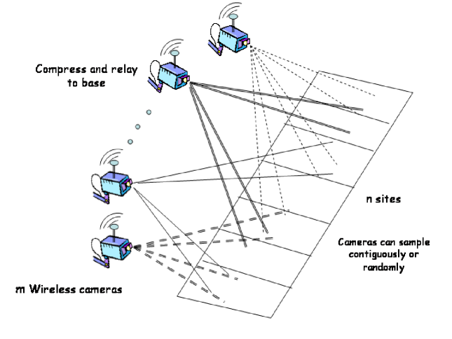
Figure 1: A schematic of I-Park: a parking lot monitoring system.

Motivated by the scenarios considered above we start with sensing (observation) models where at a sensor the information about the signal is acquired as a projection of the signal onto a weight vector. Under this class of observation model, the sensing model is linear and is essentially a matrix, $\mathbf{G}\in\mathbb{R}^{m\times n}$ chosen from some appropriate class particular to the application. In this work we consider a fixed $SNR$ model (see also [9]) where the observations at $m$ sensors for the signal $\mathbf{X}\in{\cal X}^{n}$ are given by,

$$\mathbf{Y}=\sqrt{SNR}\,\,\mathbf{G}\mathbf{X}+\mathbf{N}$$ (1)

where each row of the matrix $\mathbf{G}$ is restricted to have a unit $\ell_{2}$ norm and where $\mathbf{N}$ is the noise vector with unit noise power in each dimension. It is important to consider fixed SNR scenario particularly for applications related to sensor networks. Practically each sensor is power limited. In an active sensing scenario the sensors distribute this power to sense different modalities, or to look (beamform) in various directions. Thus we restrict the $\ell_{2}$ norm of each row of $\mathbf{G}$ to be unity and then scale the system model appropriately by $SNR$. For a networked setting we assume that the observations made at the sensors are available for processing at a centralized location or node. In case when this is infeasible or costly, information can be exchanged or aggregated at each sensor using distributed consensus type algorithms, such as that studied in [10].

In order utilize the information theoretic ideas and tools, we adopt a Bayesian perspective and assume a prior distribution on $\mathbf{X}$. Another motivation for considering a Bayesian set-up is that one can potentially model classification/detection scenarios where prior information is usually available and is useful. Note that under some technical conditions it can be shown that a lower bound to the Bayesian error is also lower bound to worst case probability of error for the parametric set-up. Therefore the lower bounds presented in this paper also provide lower bounds to the parameter estimation problem.

In this paper we capture the system performance via evaluating asymptotic upper and lower bounds to the ratio $C(d_{0})=\frac{n}{m}$ such that reconstruction to within a distortion level $d_{0}$ is feasible. We call the ratio $C(d_{0})$ as sensing capacity : the number of signal dimensions reliably identified per projection (sensor). This term was coined in [11] in the context of sensor networks for discrete applications. Alternatively, bounds to $C(d_{0})$ can be interpreted as providing scaling laws for the minimal number of sensors/projections required for reliable monitoring/signal reconstruction.

For a signal sparsity level of $k$, a different ratio of $\frac{k}{m}$ also seems to be a reasonable choice, but in most cases $k$ is unknown and needs to be determined, e.g., target density, or sparsest signal reconstruction. Here it is important to penalize false alarms, misclassification costs. Furthermore, $n$ and $m$ are known and part of the problem specification, while signal complexity is governed by $k$, and one of our goals is to understand performance as a function of signal complexity. In this paper we show that sensing capacity $C(d_{0})$ is also a function of signal sparsity apart from $SNR$.

The upper bounds to $C(d_{0})$ are derived via finding lower bounds to the probability of error in reconstruction subject to a distortion criteria, that apply to any algorithm used for reconstruction. The achievable (lower) bounds to $C(d_{0})$ are derived via upper bounding the probability of error in a max-likelihood detection set-up over the set of rate distortion quantization points. Since most of the development for these classes of problems has been algorithmic, [3, 9], our motivation for the above development is driven by the need to find fundamental algorithm independent bounds for these classes of problems. In particular, under an i.i.d model on the components of $\mathbf{X}$ that models a priori information, e.g. sparsity of $\mathbf{X}$, and letting $\hat{\mathbf{X}}(\mathbf{Y})$ denote the reconstruction of $\mathbf{X}$ from $\mathbf{Y}$, then we show that,

$$Pr\left(\frac{1}{n}d(\hat{\mathbf{X}}(\mathbf{Y}),\mathbf{X})\geq d_{0}\right)\geq\dfrac{R_{X}(d_{0})-K(d_{0},n)-\frac{1}{n}I(\mathbf{X};\mathbf{Y}|\mathbf{G})}{R_{X}(d_{0})}-o(1)$$ (2)

for some appropriate distortion measure $d(.,.)$ and where $R_{X}(d_{0})$ is the corresponding scalar rate distortion function; $K(n,d_{0})$ is bounded by a constant and it depends on the number of neighbors of a quantization point in an optimal $n-$dimensional rate distortion mapping.

Next, we consider the effect of structure of $\mathbf{G}$ on the performance. Using the result on the lower bound on the probability of error given by equation (2), a necessary condition is immediately identified in order that the reconstruction to within an average distortion level $d_{0}$ is feasible, which is, $R_{X}(d_{0})-K(n,d_{0})\leq\dfrac{1}{n}I(\mathbf{X};\mathbf{Y}|\mathbf{G})$. For a fixed prior on $\mathbf{X}$ the performance is then determined by the mutual information term that in turn depends on $\mathbf{G}$. This motivates us to consider the effect of the structure of $\mathbf{G}$ on the performance and via evaluation of $I(\mathbf{X};\mathbf{Y}|\mathbf{G})$ for various ensembles of $\mathbf{G}$ we quantify the performance of many different scenarios that restrict the choice of $\mathbf{G}$ for sensing. Under the case when $\mathbf{G}$ is chosen independently of $\mathbf{X}$ and randomly from an ensemble of matrices (to be specified later in the problem set-up), we have

$$I(\mathbf{X};\mathbf{Y},\mathbf{G}) = \underset{=0}{\underbrace{I(\mathbf{X};\mathbf{G})}}+I(\mathbf{X};\mathbf{Y}|\mathbf{G})$$ (3)

$$= I(\mathbf{X};\mathbf{Y})+I(\mathbf{X};\mathbf{G}|\mathbf{Y})$$ (4)

$$\Rightarrow I(\mathbf{X};\mathbf{Y}|\mathbf{G}) = I(\mathbf{X};\mathbf{Y})+I(\mathbf{X};\mathbf{G}|\mathbf{Y})$$ (5)

This way of expanding allow us to isolate the effect of structure of the sensing matrix $\mathbf{G}$ on the performance which in principle influences bounds on $C(d_{0})$ through the change in mutual information as captured via the equations 3-5 and as applied to satisfy the necessary conditions prescribed by the lower bound in equation (2).

Using the above idea, in this paper we will show the effect of sensing diversity on the performance, a concept which is explained next. Under the sensing model as prescribed above, at each sensor one can relate each component of the corresponding projection vector as contributing towards diversity in sensing. The total number of non-zero components in the projection vector is called sensing diversity. This terminology is analogous to that used in MIMO systems in the context of communications. As will be shown later on that loss in sensing capacity is not very significant at reasonable levels of sensing diversity (with randomization in sampling per sensor). In fact there is a saturation effect that comes into play, which implies that most of the gains can be obtained at diversity factor close to $0.5$. Now if one considers the noiseless case, i.e. $\mathbf{Y}=\mathbf{G}\mathbf{X}$, then it was shown in [3] that for some $m$ and for some sparsity $k$ as a function of $n$ and the coherence of the sensing matrix, an $\ell_{1}$ optimization problem :

$$\begin{array}[]{l}\min||\mathbf{X}||_{1}\\ \mbox{subject to}:\,\,\mathbf{Y}=\mathbf{G}\mathbf{X},\,\,\mathbf{X}\geq 0\end{array}$$

yields exact solution. To this end note that if $\mathbf{G}$ is sparse then solving the above system is computationally faster as is shown in [12].

There are other types of modalities that arise in the context of resource constrained sensor networks. As an example consider the application in [7] where each camera may be physically restricted to sample contiguous locations in space or under limited memory it is restricted to sample few locations, possibly at random. This motivates us to consider other structures on $\mathbf{G}$ under such modalities of operation. In this paper we will contrast random sampling and contiguous sampling and show that random sampling is better than contiguous sampling. In such scenarios it becomes important to address a coverage question and in some cases may lead to a poor performance. In highly resource constrained scenarios randomization in elements of $\mathbf{G}$ is not feasible. In this direction we also consider an ensemble of $\left\{0,1\right\}$ matrices, with and without randomization in the locations of non-zero entries in each row. To facilitate the reading of the paper we itemize the organization as follows.

• We present the problem set-up in section II where we make precise the signal models and the ensembles of sensing matrices that will be considered in relation to different sensor networking scenarios.

• In section III we will present the lower bounds to the probability of error in reconstruction subject to an average distortion criteria. The development is fairly general and is self-contained.

• In section IV we will present a constructive upper bound to the probability of error in reconstruction subject to an average $\ell_{2}$ distortion criteria. The development there is particular to the fixed SNR linear sensing model that is the subject of the present paper, though the ideas are in general applicable to other sensing models and to other classes of distortion measures.

• Once we establish the upper and lower bounds, we will use the results to obtain upper and lower bounds to sensing capacity for the fixed SNR linear sensing models, in sections V and VI. In these sections we will consider the full diversity Gaussian ensemble for sensing matrix. The motivation to consider this model is that the mutual information and moment generating functions are easier to evaluate for the Gaussian ensemble. This is thus useful to gain initial insights into the tradeoffs of signal sparsity and SNR.

• Since the bounds to sensing capacity can be interpreted as providing bounds for number of projections/sensors for reliable monitoring, in section VII we will compare the scaling implied by bounds to sensing capacity to that obtained in [9] in the context of complexity penalized regularization framework.

• In section VIII we consider the effect of the structure of the sensing matrix $\mathbf{G}$ on sensing capacity. The section is divided into several subsections. We begin by considering the effect of sensing diversity on sensing capacity. Following that we consider the effect of correlation in the columns of $\mathbf{G}$ on achievable sensing capacity. Then we consider a very general case of a deterministic sensing matrix and via upper bounding the mutual information we comment on the performance of various types of sensing architectures of interest.

• In section IX we consider the $\left\{0,1\right\}$ ensemble for sensing matrices and provide upper bounds to sensing capacity for various modalities in sensing.

• In section X we give an example of how our methods can be extended to handle cases when one is interested in reconstruction of functions of $\mathbf{X}$ rather than $\mathbf{X}$ itself. In this direction we will consider the case of recovery of sign patterns of $\mathbf{X}$.

II Problem Set-up

Assume that the underlying signal $\mathbf{X}$ lies in an n-dimensional space ${\cal X}^{n}$, where ${\cal X}$ can be discrete or continuous. Discrete ${\cal X}$ models scenarios of detection or classification and continuous ${\cal X}$ models scenarios of estimation.

Fixed SNR model

: The observation model for the sensors is a linear observation model and is given by,

$$\mathbf{Y}=\sqrt{SNR}\,\,\mathbf{G}\mathbf{X}+\mathbf{N}$$ (6)

which is the fixed $SNR$ model as described in the introduction. The matrix $\mathbf{G}\in\mathbb{R}^{m\times n}$ is a random matrix selected from an ensemble which we will state subsequently. For all $m,n$ each row of $\mathbf{G}$ is restricted to have a unit $\ell_{2}$ norm. The noise vector $\mathbf{N}$ is i.i.d. Gaussian unit variance in each dimension.

II-A Discussion about fixed SNR model

At this point it is important to bring out an important distinction of the assumption and subsequently analysis of a fixed SNR model in contrast to similar scenarios considered but in albeit high SNR setting. The observation model of equation 1 studied in this paper is related to a class of problems that have been central in statistics. In particular it is related to the problem of regression for model order selection. In this context the subsets of columns of the sensing matrix $\mathbf{G}$ form a model for signal representation which needs to be estimated from the given set of observations. The nature selects this subset in a weighted/non-weighted way as modeled by $\mathbf{X}$. The task is then to estimate this model order and thus $\mathbf{X}$. In other words estimate of $\mathbf{X}$ in most cases is also linked to the estimate of the model order under some mild assumptions on $\mathbf{G}$. Several representative papers in this direction are [13, 14, 15] that consider the performance of several (signal) complexity penalized estimators in both parametric and non-parametric framework. One of the key differences to note here is that the analysis of these algorithms is done for the case when $SNR\rightarrow\infty$, i.e. in the limit of high SNR which is reflected by taking the additive noise variance to go to zero or not considering the noise at all. However SNR is an important and necessary ingredient for applications related to sensor networks and therefore we will not pursue a high SNR development here. Nevertheless the results obtained are directly applicable to such scenarios.

In the next section we will first outline prior distribution(s) on $\mathbf{X}$, that reflect the sparsity of the signal $\mathbf{X}$ and the model for realizing sensing diversity in the sensing matrix $\mathbf{G}$. Then we will outline the choices of ensembles for the sensing matrix $\mathbf{G}$. In the following ${\cal N}(m,\sigma^{2})$ denotes the Gaussian distribution with mean $m$ and variance $\sigma^{2}$.

II-B Generative models of signal sparsity and sensing diversity

Signal sparsity

In a Bayesian set-up we model the sparsity of the phenomena by assuming a mixture distribution on the signals $\mathbf{X}$. In particular the $n$ dimensional vector $\mathbf{X}=X_{1},...,X_{n}$ is a sequence drawn i.i.d from a mixture distribution

$$P_{X}=\alpha{\cal N}(m_{1},\sigma_{1}^{2})+(1-\alpha){\cal N}(m_{0},\sigma_{0}^{2})$$

where $\alpha\leq\frac{1}{2}$. In this paper we consider two cases.

1. Discrete Case: $m_{1}=1$ and $m_{0}=0$ and $\sigma_{1}=\sigma_{0}=0$. This means that $\mathbf{X}$ is a Bernoulli$(\alpha)$ sequence. This models the discrete case for addressing problems of target localization, search, etc.

2. Continuous Case: $m_{1}=m_{2}=0$ but $\sigma_{1}^{2}=1$ and $\sigma_{0}^{2}=0$. This models the continuous case.

In this context we call $\alpha$ the sparsity ratio which is held fixed for all values of $n$. Under the above model, on an average the signal will be $k$ sparse where $k=\alpha n$. Note that $k\rightarrow\infty$ as $n\rightarrow\infty$.

Sensing diversity and ensemble for $\mathbf{G}$

In connection to the model for diversity, the sensing matrix $\mathbf{G}$ is random matrix such that for each row $i$, $\mathbf{G}_{ij},j=1,2,..,n$ are distributed i.i.d according to a mixture distribution, $(1-\beta){\cal N}(m_{0},\sigma_{0}^{2})+\beta{\cal N}(m_{1},\sigma_{1}^{2})$. We consider three cases:

1. Gaussian ensemble: $m_{1}=m_{0}=0$ and $\sigma_{1}=1;\sigma_{0}=0$

2. Deterministic $\mathbf{G}$: The matrix $\mathbf{G}$ is deterministic.

3. $\left\{0,1\right\}^{m\times n}$ ensemble: $m_{1}=1;m_{0}=0$ and $\sigma_{1}=\sigma_{0}=0$.

The matrix is then normalized so that each row has a unit $\ell_{2}$ norm. In this context we call $\beta$ as the (sensing) diversity ratio. Under the above model, on an average each sensor will have a diversity of $l=\beta n$. Note that $l\rightarrow\infty$ as $n\rightarrow\infty$. Given the set-up as described above the problem is to find upper and lower bounds to

$$C(d_{0})=\limsup\left\{\frac{n}{m}:Pr\left(\frac{1}{n}d(\hat{\mathbf{X}}(\mathbf{Y}),\mathbf{X})>d_{0}\right)\rightarrow 0\right\}$$

where $\hat{\mathbf{X}}(\mathbf{Y})$ is the reconstruction of $\mathbf{X}$ from observation $\mathbf{Y}$ and where $d(\mathbf{X},\hat{\mathbf{X}}(\mathbf{Y})=\sum_{i=1}^{n}d(X_{i},\hat{X}_{i}(\mathbf{Y}))$ for some distortion measure $d(.,.)$ defined on ${\cal X}\times{\cal X}$. In this paper we will consider Hamming distortion measure for discrete $\mathbf{X}$ and squared distortion measure for the continuous $\mathbf{X}$. Under this set-up we exhibit the following main results:

1. Sensing capacity $C(d_{0})$ is also a function of $SNR$, signal sparsity and sensing diversity.

2. For a fixed SNR sensing capacity goes to zero as sparsity goes to zero.

3. Low diversity implies low sensing capacity.

4. Correlations across the columns and across the rows of $\mathbf{G}$ leads to decrease in sensing capacity.

5. For the $\left\{0,1\right\}$ ensemble for sensing matrices, sensing capacity for random sampling is higher than for contiguous sampling.

In the next section we will provide asymptotic lower bounds on the probability of error in reconstruction subject to a distortion criteria. Following that we will provide a constructive upper bound to the probability of error. We will then use these results to evaluate upper and lower bounds to sensing capacity. In the following we will use $\mathbf{X}$ and $X^{n}$ interchangeably.

III Bounds to the performance of estimation algorithms: lower bounds

Lemma III.1

Given observation(s) $\mathbf{Y}$ for the sequence $X^{n}\triangleq\left\{X_{1},...,X_{n}\right\}$ of random variables drawn i.i.d. according to $P_{X}$. Let $\hat{X}^{n}(\mathbf{Y})$ be the reconstruction of $X^{n}$ from $\mathbf{Y}$. Also is given a distortion measure $d(X^{n},\hat{X}^{n}(\mathbf{Y}))=\sum_{i=1}^{n}d(X_{i},\hat{X}_{i}(\mathbf{Y}))$ then,

$$\begin{array}[]{l}Pr\left(\frac{1}{n}d(\hat{X}^{n}(\mathbf{Y}),X^{n})\geq d_{0}\right)\geq\dfrac{R_{X}(d_{0})-K(d_{0},n)-\frac{1}{n}I(X^{n};\mathbf{Y})}{R_{X}(d_{0})}-o(1)\end{array}$$

where $K(d_{0},n)$ is bounded by a constant and where $R_{X}(d_{0})$ is the corresponding (scalar) rate distortion function for $X$.

Proof:

See Appendix. ∎

Essentially, $K(n,d_{0})=\frac{1}{n}\times\log(\sharp$ neighbors of a quantization point in an optimal n-dimensional rate-distortion mapping). NOTE: The assumption of a scalar valued process in lemma III.1 is taken for the sake of simplicity. The results are easily generalizable and can be extended to the case of vector valued processes.

For the simpler case of discrete parameter space, the lower bound to the minimax error in a parameter estimation framework is related to the Bayesian error as follows,

$$\min_{\hat{\mathbf{X}}(\mathbf{Y})}\max_{\mathbf{X}\in\Theta}Pr\left(\frac{1}{n}d(\mathbf{X},\hat{\mathbf{X}}(Y))\geq d_{0}\right) = \min_{\hat{\mathbf{X}}(\mathbf{Y})}\max_{P_{\Theta}\in{\cal P}_{\theta}}\sum_{\mathbf{X}\in\Theta}P(\mathbf{X})Pr\left(\frac{1}{n}d(\mathbf{X},\hat{\mathbf{X}}(Y))\geq d_{0}\right)$$ (7)

$$\geq \min_{\hat{\mathbf{X}}(\mathbf{Y})}\sum_{\mathbf{X}\in\Theta}\pi(\mathbf{X})Pr\left(\frac{1}{n}d(\mathbf{X},\hat{\mathbf{X}}(Y))\geq d_{0}\right)$$ (8)

where $\Theta$ is the parameter space and ${\cal P}_{\Theta}$ is the class of probability measures over $\Theta$ and $\pi\in{\cal P}$ is any particular distribution. The above result holds true for the case of continuous parameter space under some mild technical conditions. Thus a lower bound to the probability of error as derived in this paper also puts a lower bound on the probability of error for the parametric set-up. In our set-up we will choose $\pi$ as a probability distribution that appropriately models the a priori information on $\mathbf{X}$, e.g. signal sparsity. For modeling simple priors such as sparsity on $\mathbf{X}$ one can choose distributions that asymptotically put most of the mass uniformly over the relevant subset of $\Theta$ and is a key ingredient in realization of the lower bound on probability of error derived in this paper.

We have the following corollary that follows from lemma III.1.

Corollary III.1

Let $X^{n}=X_{1},..,X_{n}$ be an i.i.d. sequence where each $X_{i}$ is drawn according to some distribution $P_{X}(x)$ and $X^{n}\in{\cal X}^{n}$, where $|{\cal X}|$ is finite. Given observation $\mathbf{Y}$ about $X^{n}$ we have,

$$Pr(X^{n}\neq\hat{X}^{n}(\mathbf{Y}))\geq\frac{H(X)-\frac{1}{n}I(X^{n};\mathbf{Y})-1/n}{H(X)+o(1)}-o(1)$$

III-A Tighter bounds for discrete ${\cal X}$ under hamming distortion

The results in the previous section can be stated for any finite $n$ without resorting to the use of AEP for the case of discrete alphabets, with hamming distortion as the distortion measure and for certain values of the average distortion constraint $d_{0}$. We have the following lemma.

Lemma III.2

Given observation(s) $\mathbf{Y}$ for the sequence $X^{n}\triangleq\left\{X_{1},...,X_{n}\right\}$ of random variables drawn i.i.d. according to $P_{X}$. Then for hamming under distortion measure $d_{H}(.,.)$, for $X_{i}\in{\cal X},\,\,|{\cal X}|<\infty$ and for distortion levels, $d_{0}\leq(|{\cal X}|-1)\min_{X\in{\cal X}}P_{X}$,

$$\begin{array}[]{l}Pr(\frac{1}{n}d_{H}(X^{n},\hat{X}^{n}(\mathbf{Y})\geq d_{0}))\geq\dfrac{nR_{X}(d_{0})-I(X^{n};\mathbf{Y})-1}{n\log(|{\cal X}|)-n\left(h(d_{0})+d_{0}\log(|{\cal X}|-1)\right)}\end{array}$$

Proof:

See Appendix. ∎

III-B Comment on the proof technique

The proof of lemma III.1 closely follows the proof of Fano’s inequality [16], where we start with a distortion error event based on $\frac{1}{n}d(\hat{\mathbf{X}}(\mathbf{Y}),\mathbf{X})\geq d_{0}$ and then evaluate conditional entropy of a rate-distortion mapping conditioned on the error event and the observation $\mathbf{Y}$. To bound $K(n,d_{0})$, we use results in [17] for the case of squared distortion measure.

In relation to the lower bounds presented in this paper for the probability of reconstruction subject to an average distortion level one such development was considered in [18] in the context of a non-parametric regression type problem. Let $\theta$ be an element of the metric space $(d,\Theta)$. Then given $\left\{Y_{i},\mathbf{G}_{i}\right\}_{i=1}^{m}$ for some random or non-random vectors $\mathbf{G}_{i}\in\mathbb{R}^{n}$ and $Y_{i}$ being the responses to these vectors under $\theta$. Also is given the set of conditional pdfs given by $p_{\theta(\mathbf{G}_{i})}(Y_{i})$ where the notation means that that the pdfs are parametrized by $\theta(\mathbf{G}_{i})$. The task is to find a lower bound on the minimax reconstruction distortion under measure $d$, in reconstruction of $\theta$ given $\mathbf{Y}$ and $\mathbf{G}$. In our case one can identify $\mathbf{X}\triangleq\theta$ and $\Theta\triangleq{\cal X}^{n}$ with squared metric $d$. For such a set-up lower bounds on the asymptotic minimax expected distortion in reconstruction (not the probability of such an event) was derived in [18] using a variation of Fano’s bound (see [19]) under a suitable choice of worst case quantization for the parameter space $\Theta=\left\{\mbox{space of q-smooth functions in}\,\,[0,1]^{n}\right\}$ meterized with $\ell_{r},\,1\leq r\leq\infty$ distance.

Our derivation has a flavor of this method in terms of identifying the right quantization, namely the rate distortion quantization for a given level of average distortion in a Bayesian setting. Although we evaluate the lower bounds to the probability of error and not the expected distortion itself, the lower bound on the expected distortion in reconstruction follows immediately. Moreover our method works for any distortion metric $d$, though in this paper we will restrict ourselves to cases of interest particular to sensor networks applications.

IV Constructive upper bound to the probability of error

In this section we will provide a constructive upper bound to the probability of error in reconstruction subject to an average squared distortion level. Unlike the lower bounds in this section we will provide upper bounds for the particular observation model of equation (6). This could potentially be generalized but we will keep our focus on the problem at hand.

To this end, given $\epsilon>0$ and $n$, assume that we are given the functional mapping $f(X^{n})$ (or $f(\mathbf{X})$) that corresponds to the minimal cover at average distortion level $d_{0}$ as given by lemma XI.2. Upon receiving the observation $\mathbf{Y}$ the aim is to map it to the index corresponding index $f(\mathbf{X})$, i.e. we want to detect which distortion ball the true signal belongs to. Clearly if $\mathbf{X}$ is not typical there is an error. From lemma XI.1, the probability of this event can be bounded by an arbitrary $\delta>0$ for a large enough n. So we will not worry about this a-typical event in the following.

Since all the sequences in the typical set are equiprobable, we covert the problem to a max-likelihood detection set-up over the set of rate-distortion quantization points given by the minimal cover as follows. Given $\mathbf{G}$ we and the rate distortion points corresponding to the functional mapping $f(X^{n})$, we enumerate the set of points, $\mathbf{G}Z_{i}^{n}\in\mathbb{R}^{m}$. Then given the observation $\mathbf{Y}$ we map $\mathbf{Y}$ to the nearest point (in $\mathbb{R}^{m}$) $\mathbf{G}Z_{i}^{n}$. Then we ask the following probability,

$$\begin{array}[]{l}Pr\left(\sqrt{SNR}\mathbf{G}f(\mathbf{X})\rightarrow\sqrt{SNR}\mathbf{G}f(\mathbf{X}^{\prime})|\mathbf{G},\mathbf{X}\in\mathcal{B}_{i},\mathbf{X}^{\prime}\in\mathcal{B}_{j}:\frac{1}{n}d_{set}(\mathcal{B}_{i},\mathcal{B}_{j})\geq 2d_{0}\right)\par\end{array}$$

that is, we are asking what is the probability that the in typical max-likelihood detection set-up we will map signals from distortion ball $\mathcal{B}_{i}$ to signals in distortion ball $\mathcal{B}_{j}$ that is at an average set distance $\geq 2d_{0}$ from $\mathcal{B}_{i}$, where $d_{set}(\mathcal{B}_{i},\mathcal{B}_{j})=\min_{\mathbf{X}\in\mathcal{B}_{i},\mathbf{X}^{\prime}\in\mathcal{B}_{j}}d(\mathbf{X},\mathbf{X}^{\prime})$. For sake of brevity we denote the above probability via $P_{e}(pair)$ to reflect it as a pairwise error probability. Since the noise is additive Gaussian noise we have

$$P_{e}(pair)=Pr\left(\mathbf{N}^{T}\mathbf{G}(\mathbf{X}-\mathbf{X}^{\prime})\geq\frac{1}{2}\sqrt{SNR}||\mathbf{G}(\mathbf{X}-\mathbf{X}^{\prime})||^{2}\,\,\,:\mathbf{X}\in\mathcal{B}_{i},\mathbf{X}^{\prime}\in\mathcal{B}_{j}\right)$$

$$P_{e}(pair)=Pr\left(\mathbf{N}^{T}\frac{\mathbf{G}(\mathbf{X}-\mathbf{X}^{\prime})}{||\mathbf{G}(\mathbf{X}-\mathbf{X}^{\prime})||}\geq\frac{\sqrt{SNR}}{2||\mathbf{G}(\mathbf{X}_{1}-\mathbf{X}_{2})||}||\mathbf{G}(\mathbf{X}-\mathbf{X}^{\prime})||^{2}\,\,\,:\mathbf{X}\in\mathcal{B}_{i},\mathbf{X}^{\prime}\in\mathcal{B}_{j}\right)$$

Since noise $\mathbf{N}$ is AWGN noise with unit variance in each dimension, its projection onto the unit vector $\frac{\mathbf{G}(\mathbf{X}-\mathbf{X}^{\prime})}{||\mathbf{G}(\mathbf{X}-\mathbf{X}^{\prime})||}$ is also Gaussian with unit variance. Thus we have

$$P_{e}(pair)=Pr\left(N\geq\frac{\sqrt{SNR}}{2}||\mathbf{G}(\mathbf{X}-\mathbf{X}^{\prime})||\,\,\,:\mathbf{X}\in\mathcal{B}_{i},\mathbf{X}^{\prime}\in\mathcal{B}_{j}\right)$$

By a standard approximation to the ${\cal Q}(.)$ (error) function, we have that,

$$P_{e}\left(f(\mathbf{X})\rightarrow f(\mathbf{X}^{\prime})|\mathbf{X}\in\mathcal{B}_{i},\mathbf{X}^{\prime}\in\mathcal{B}_{j},\mathbf{G}\,\,:\frac{1}{n}d_{set}(\mathcal{B}_{i},\mathcal{B}_{j})\geq 2d_{0}\right)\leq\exp\left\{-\dfrac{SNR||\mathbf{G}(\mathbf{X}-\mathbf{X}^{\prime})||^{2}}{4}\right\}$$

In the worst case we have the following bound,

$$P_{e}\left(f(\mathbf{X})\rightarrow f(\mathbf{X}^{\prime})|\mathbf{X}\in\mathcal{B}_{i},\mathbf{X}^{\prime}\in\mathcal{B}_{j},\mathbf{G}\,\,:\frac{1}{n}d_{set}(\mathcal{B}_{i},\mathcal{B}_{j})\geq 2d_{0}\right)\leq\exp\left\{-\min_{\mathbf{X}\in\mathcal{B}_{i},\mathbf{X}^{\prime}\in\mathcal{B}_{j}}\dfrac{SNR||\mathbf{G}(\mathbf{X}-\mathbf{X}^{\prime})||^{2}}{4}\right\}$$

Now note that from above construction it implies that the average distortion in reconstruction of $\mathbf{X}$ is bounded by $2d_{0}$ if the distortion metric obeys triangle inequality. To evaluate the total probability of error we use the union bound to get,

$$Pr\left(\frac{1}{n}d(\mathbf{X},\hat{\mathbf{X}}(\mathbf{Y}))\geq 2d_{0}\right)\leq\exp\left\{-\min_{\mathbf{X}\in\mathcal{B}_{i},\mathbf{X}^{\prime}\in\mathcal{B}_{j}}\dfrac{SNR||\mathbf{G}(\mathbf{X}-\mathbf{X}^{\prime})||^{2}}{4}\right\}2^{n(R_{X}(d_{0})-K(n,d_{0}))}$$

We will use this general form and apply it to particular cases of ensembles of the sensing matrix $\mathbf{G}$. In the following sections we begin by providing upper and lower bounds to the sensing capacity for the Gaussian ensemble for full diversity.

V Sensing Capacity: Upper bounds, Gaussian ensemble

V-A Discrete $\mathbf{X}$, full diversity, Gaussian ensemble

For this case we have the following main lemma.

Lemma V.1

Given $\mathbf{X}\in\left\{0,1\right\}^{n}$ drawn Bernoulli $(\alpha,1-\alpha)$ and $\mathbf{G}$ chosen from the Gaussian ensemble. Then, with the distortion measure as the hamming distortion, for a diversity ratio of $\beta=1$ and for $d_{0}\leq\alpha$, the sensing capacity $C$ is upper bounded by

$$C(d_{0})\leq\dfrac{\frac{1}{2}\log(1+\alpha SNR)}{R_{X}(d_{0})}$$

Proof:

From lemma III.2 the probability of error is lower bounded by zero if the numerator in the lower bound is negative, this implies for any $m,n$ that

$$C_{m,n}(d_{0},\mathbf{G})\leq\dfrac{\frac{1}{m}I(\mathbf{X};\mathbf{Y}|\mathbf{G})}{R_{X}(d_{0})}$$

Since $\mathbf{G}$ is random we take expectation over $\mathbf{G}$. It can be shown that the mutual information

$$\begin{array}[]{l}\mathbf{E}_{\mathbf{G}}I(X^{n};\mathbf{Y}|\mathbf{G})\leq\\ \max_{P_{\mathbf{X}}:\sum\frac{1}{n}\mathbf{E}X_{i}^{2}\leq\alpha}\frac{1}{2}\mathbf{E}_{\mathbf{G}}\log det(\mathbf{I}_{m\times m}+\mathbf{G}\mathbf{X}\mathbf{X}^{T}\mathbf{G}^{T})\end{array}$$

$=\mathbf{E}_{\lambda_{1},..,\lambda_{m}}\sum_{i=1}^{m}\frac{1}{2}\log(1+\lambda_{i}\alpha SNR)$ where $\lambda_{i}$ are singular values of $\mathbf{G}\mathbf{G}^{T}$. Since rows of $\mathbf{G}$ have a unit norm $\Rightarrow\lambda_{i}\leq 1\,\,\forall i$. Hence $\mathbf{E}_{\mathbf{G}}I(X^{n};\mathbf{Y}|\mathbf{G})\leq\frac{m}{2}\log(1+\alpha SNR)$. Thus the result follows. ∎

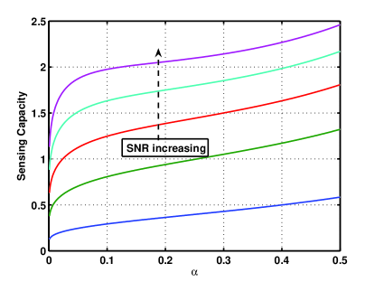
Figure 2: The plot of sparsity versus upper bounds to the sensing capacity for various SNRs for the binary case ($\mathcal{X}=\{0,1\}$) for zero Hamming distortion.

V-B Continuous $\mathbf{X}$, full diversity, Gaussian ensemble

Lemma V.2

Given $\mathbf{X}\in\mathbb{R}^{n}$ drawn i.i.d. according to $P_{X}=\alpha{\cal N}(0,1)+(1-\alpha){\cal N}(0,0)$ and $\mathbf{G}$ chosen from the Gaussian ensemble. Then, for squared distortion measure, for diversity ratio $\beta=1$ and for $d_{0}\leq\frac{\alpha}{2}$, the sensing capacity $C(d_{0})$ obeys,

$$C(d_{0})\leq\dfrac{\frac{1}{2}\log(1+\alpha SNR)}{H(\alpha)+\frac{\alpha}{2}\log\frac{\alpha}{2d_{0}}}$$

Proof:

From lemma V.1 we have that $\mathbf{E}_{\mathbf{G}}I(\mathbf{X};\mathbf{Y}|\mathbf{G})\leq\frac{m}{2}\log(1+\alpha SNR)$. In order that the probability of error be lower bounded by zero, from lemma III.1 it follows that asymptotically

$$\frac{n}{m}\leq\frac{\mathbf{E}_{\mathbf{G}}I(\mathbf{X};\mathbf{Y}|\mathbf{G})}{R_{X}(d_{0})-K(d_{0},n)}$$

It can be shown that $|K(d_{0},n)-\log 2|<\epsilon$ with $\epsilon$ very small for large enough $n$, see e.g. [17]. The lemma then follows by plugging in the results from section XI-C. ∎

It can be easily seen that as $\alpha\downarrow 0$ the sensing capacity goes to zero. We illustrate this by plotting the upper bounds in figure 2 for the discrete case. We will revisit this phenomena in section VII in relation to the bounds derived in [5] in the context of compressed sensing.

VI Sensing Capacity: Lower bounds, Gaussian ensemble

VI-A Discrete alphabet, full diversity

The discrete $\mathbf{X}$ with hamming distortion is a special case where we can provide tighter upper bounds. The proof follows from the development in section IV and identifying that for the discrete case one can choose the discrete set of points instead of the distortion balls. We have the following lemma.

Lemma VI.1

Given $\mathbf{X}\in{\cal X}^{n}$ with $|{\cal X}|<\infty$, for $\beta=1$ and $\mathbf{G}$ chosen from a Gaussian ensemble. Then for $d_{0}\leq\min_{x\in{\cal X}}P_{X}(x)$, a sensing capacity of

$$C(d_{0})=\dfrac{\frac{1}{2}\log(1+\frac{SNRd_{0}}{2})}{H(X)-d_{0}\log|{\cal X}-1|-d_{0}\log\frac{1}{d_{0}}}$$

is achievable in that the probability of error goes down to zero exponentially for choices of $C=\frac{n}{m}=C(d_{0})-\eta$ for any $\eta>0$.

Proof:

We have

$$Pr\left(\frac{1}{n}d(\mathbf{X},\hat{\mathbf{X}}(\mathbf{Y}))\geq d_{0}|\mathbf{G}\right)\leq\exp\left\{-\dfrac{SNR||\mathbf{G}(\mathbf{X}-\mathbf{X}^{\prime})||^{2}}{4}\right\}2^{nH(X)-nd_{0}\log|{\cal X}-1|-\log\binom{n}{nd_{0}}}$$

where we have applied the union bound to all the typical sequences that are outside the hamming distortion ball of radius $d_{0}$. Taking the expectation with respect to $\mathbf{G}$ we get,

$$Pr\left(\frac{1}{n}d(\mathbf{X},\hat{\mathbf{X}}(\mathbf{Y}))\geq d_{0}\right)\leq\mathbf{E}_{\mathbf{G}}\exp\left\{-\dfrac{SNR||\mathbf{G}(\mathbf{X}-\mathbf{X}^{\prime})||^{2}}{4}\right\}2^{nH(X)-nd_{0}\log|{\cal X}-1|-\log\binom{n}{nd_{0}}}$$

Now note that since $\mathbf{G}$ is a Gaussian random matrix where each row has a unit $\ell_{2}$ norm, $||\mathbf{G}(\mathbf{X}-\mathbf{X}^{\prime})||^{2}=\sum_{i=1}^{m}|\sum_{j=1}^{n}\mathbf{G}_{ij}(X_{i}-X^{\prime}_{j})|^{2}$ is a sum of $m$ independent $\chi^{2}$ random variables with mean $||\mathbf{X}-\mathbf{X}^{\prime}||^{2}$. Thus from the moment generating function of the $\chi^{2}$ random variable we get that,

$$Pr\left(\frac{1}{n}d(\mathbf{X},\hat{\mathbf{X}}(\mathbf{Y}))\geq d_{0}\right)\leq\left(\dfrac{1}{1+\frac{SNR||\mathbf{X}-\mathbf{X}^{\prime}||^{2}}{2\,n}}\right)^{m/2}2^{nH(X)-nd_{0}\log|{\cal X}-1|-\log\binom{n}{nd_{0}}}$$

This implies,

$$Pr\left(\frac{1}{n}d(\mathbf{X},\hat{\mathbf{X}}(\mathbf{Y}))\geq d_{0}\right)\leq 2^{-\frac{m}{2}\log(1+\frac{SNRd_{0}}{2})}2^{nH(X)-nd_{0}\log|{\cal X}-1|-\log\binom{n}{nd_{0}}}$$

Now note that for $d_{0}\leq\alpha$, $\log\binom{n}{nd_{0}}\geq nd_{0}\log\frac{1}{d_{0}}$. Then from above one can see that the probability of error goes down to zero if,

$$\frac{n}{m}<\dfrac{\frac{1}{2}\log(1+\frac{SNRd_{0}}{2})}{H(X)-d_{0}\log|{\cal X}-1|-d_{0}\log\frac{1}{d_{0}}}$$

Thus a sensing capacity of

$$C(d_{0})=\dfrac{\frac{1}{2}\log(1+\frac{SNRd_{0}}{2})}{H(X)-d_{0}\log|{\cal X}-1|-d_{0}\log\frac{1}{d_{0}}}$$

is achievable in that the probability of error goes down to zero exponentially for choices of $C=\frac{n}{m}=C(d_{0})-\eta$ for any $\eta>0$.

∎

VI-B Continuous $\mathbf{X}$, full diversity

Lemma VI.2

[Weak Achievability] For $\mathbf{X}\in\mathbb{R}^{n}$ and drawn i.i.d. according to $P_{x}(X)$, $\mathbf{G}$ chosen from the Gaussian ensemble and $\beta=1$, a sensing capacity of

$$C(2d_{0})=\dfrac{\frac{1}{2}\log(1+d_{0}SNR)}{R_{X}(d_{0})-K(n,d_{0})}$$

is achievable in that the probability of error goes down to zero exponentially with $n$ for $C=\frac{n}{m}\leq C(2d_{0})-\epsilon$ for some arbitrary $\epsilon>0$.

Proof:

For this case we invoke the construction as outlined in section IV. From the results in that section we get that,

$$Pr\left(\frac{1}{n}d(\mathbf{X},\hat{\mathbf{X}}(\mathbf{Y}))\geq 2d_{0}\right)\leq\exp\left\{-\min_{\mathbf{X}\in\mathcal{B}_{i},\mathbf{X}^{\prime}\in\mathcal{B}_{j}}\dfrac{SNR||\mathbf{G}(\mathbf{X}-\mathbf{X}^{\prime})||^{2}}{4}\right\}2^{n(R_{X}(d_{0})-K(n,d_{0}))}$$

Note that the result is little weaker in that guarantees are only provided to reconstruction within $d_{0}$, but one can appropriately modify the rate distortion codebook to get the desired average distortion level. Proceeding as in the case of discrete $\mathbf{X}$ and , by taking the expectation over $\mathbf{G}$ and noting that $\min_{\mathbf{X}\in\mathcal{B}_{i},\mathbf{X}^{\prime}\in\mathcal{B}_{j}}||\mathbf{X}-\mathbf{X}^{\prime}||^{2}\geq 2nd_{0}$, we get that,

$$Pr\left(\frac{1}{n}d(\mathbf{X},\hat{\mathbf{X}}(\mathbf{Y}))\geq 2d_{0}\right)\leq\left(\dfrac{1}{1+SNRd_{0}}\right)^{m/2}2^{n(R_{X}(d_{0})-K(n,d_{0}))}$$

This implies,

$$Pr\left(\frac{1}{n}d(\mathbf{X},\hat{\mathbf{X}}(\mathbf{Y}))\geq 2d_{0}\right)\leq\left(\dfrac{1}{1+SNRd_{0}}\right)^{m/2}2^{n(R_{X}(d_{0})-K(n,d_{0}))}$$

$$Pr\left(\frac{1}{n}d(\mathbf{X},\hat{\mathbf{X}}(\mathbf{Y}))\geq 2d_{0}\right)\leq 2^{-\frac{m}{2}\log(1+SNRd_{0})}2^{n(R_{X}(d_{0})-K(n,d_{0}))}$$

This implies that for

$$\frac{n}{m}<\dfrac{\frac{1}{2}\log(1+d_{0}SNR)}{R_{X}(d_{0})-K(n,d_{0})}$$

the probability of error goes to zero exponentially. This means that a sensing capacity of

$$C(2d_{0})=\dfrac{\frac{1}{2}\log(1+d_{0}SNR)}{R_{X}(d_{0})-K(n,d_{0})}$$

is achievable in that the probability of error goes down to zero exponentially with $n$ for $C=\frac{n}{m}\leq C(d_{0})-\eta$ for some arbitrary $\eta>0$.

∎

A plot of upper and lower bounds are shown in figure 3.

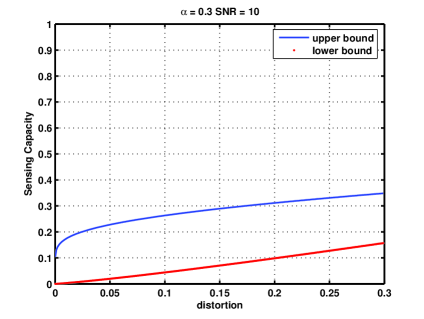
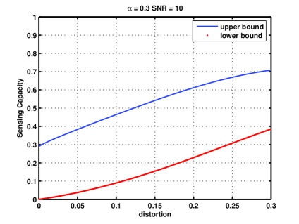
(a) (b)

Figure 3: (a) Plots of upper and lower bounds to sensing capacity for the Gaussian mixture model. (b) Plots of upper and lower bounds for sensing capacity for the Bernoulli model. The distortion on the x-axis is mean squared distortion for the Gaussian case and hamming distortion for the Bernoulli case. Note that zero distortion achievable sensing capacity is zero and there is an SNR gap in the upper and lower bounds.

VII Comparison with existing bounds

Note that the results in this paper are stated for $d_{0}\leq\alpha$ for the discrete case and for $d_{0}\leq\frac{\alpha}{2}$ for the continuous case. This is because one must consider stricter average distortion measures as the phenomena becomes sparser. To bring out this point concretely and for purposes of comparison with existing bounds, we consider the result obtained in [5] based on optimal complexity regularized estimation framework. They show that the expected mean squared error in reconstruction is upper bounded by,

$$\mathbf{E}\left[\frac{1}{n}||\mathbf{X}-\hat{\mathbf{X}}||^{2}\right]\leq C_{1}C_{2}\frac{k\log n}{m}$$ (9)

where $C_{1}\sim 1$ and $C_{2}\sim 50(P+\sigma)^{2}\left\{(1+p)\log 2+4\right\}$, under normalization of the signal and the noise power and $p$ is the number of quantization levels, [9]. To this end consider an extremely sparse case, i.e., $k=1$. Then the average distortion metric in equation 9, does not adequately capture the performance, as one can always declare all zeros to be the estimated vector and the distortion then is upper bounded by ${\cal O}(\frac{1}{n})$. Consider the case when $\mathbf{X}$ is extremely sparse, i.e. $\alpha\downarrow 0$ as $\frac{1}{n}$. Then a right comparison is to evaluate the average distortion per number of non-zero elements, $\mathbf{E}\left[\frac{1}{\alpha n}||\mathbf{X}-\hat{\mathbf{X}}||^{2}\right]$. Using this as the performance metric we have from equation 9,

$$\mathbf{E}\left[\frac{1}{\alpha n}||\mathbf{X}-\hat{\mathbf{X}}||^{2}\right]\leq C_{1}C_{2}\frac{n\log n}{m}$$ (10)

When $\alpha$ is small then the average number of projections required such that the per non-zero element distortion is bounded by a constant, scales as ${\cal O}(n\log n)$. This is indeed consistent with our results, in that the Sensing Capacity goes down to zero as $\frac{1}{\log n}$.

$\mathbf{X}$ is sparse, i.e. $\alpha<1$ but not very small. From results on achievable sensing capacity we have that

$$\begin{array}[]{ll}Pr\left(\frac{1}{n}||\mathbf{X}-\hat{\mathbf{X}}||^{2}\geq d_{0}\right)\leq-\frac{m}{2}\log(1+d_{0}SNR/2)+n(R_{X}(d_{0})-K(n,d_{0}))\end{array}$$

In order to compare the results we fix, performance guarantee of $Pr(d(\mathbf{X},\hat{\mathbf{X}})\geq d_{0})\leq\epsilon$ for a given $\epsilon>0$, we have for the minimal number of projections required that,

$$m\geq\frac{2\left(\log(1/\epsilon)+n(R_{X}(d_{0})-K(n,d_{0}))\right)}{\log(1+d_{0}SNR/2)}$$

from our results. From results in [9] it follows that,

$$m\geq C_{1}C_{2}\frac{\alpha n\log n}{d_{0}\epsilon}$$

For the special case of binary alphabet we have the following scaling orders for the number of projections in both cases, from achievable sensing capacity we have $m_{1}\geq{\cal O}(nH_{2}(\alpha))$ and from results in [9] we have $m_{2}\geq{\cal O}(\alpha n\log n)$. A plot of these orders as a function of $\alpha$ for a fixed $n$ is shown in figure, 4.

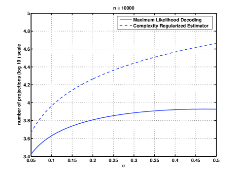
Figure 4: The difference in scaling of the number of projections with the sparsity rate from bounds derived from Sensing Capacity and from bounds obtained in [9]. Our bounds are sharper.

VIII Effect of structure of $\mathbf{G}$

In this section we will show that effect of structure of $\mathbf{G}$ on sensing capacity. This section is divided into several subsections and the discussion is self-contained. In section VIII-A we will show that for the Gaussian ensemble, the sensing capacity reduces for when diversity is low. Following that in section VIII-B we will show the effect of correlation across columns in the sensing matrix for the Gaussian ensemble on achievable sensing capacity. In section VIII-C we will present a general result for a generic sensing matrix $\mathbf{G}$ which will subsequently be used to highlight the effect of structures such as that induced via random filtering using a FIR filter with/without downsampling as considered in [20].

VIII-A Effect of sensing diversity, Gaussian ensemble

In order to show the effect of sensing diversity we evaluate the mutual information $\mathbf{E}_{\mathbf{G}}I(\mathbf{X};\mathbf{Y}|\mathbf{G})$ using the intuition described in the introduction. To this end we have the following lemma.

Lemma VIII.1

For a diversity ratio of $\beta$, with $l=\beta n$ as the average diversity per sensor and an average sparsity level of $k=\alpha n$ , we have

$$\mathbf{E}_{\mathbf{G}}I(\mathbf{X};\mathbf{Y}|\mathbf{G})\leq\frac{m}{2}\mathbf{E}_{j}\left[\log\left(\frac{SNR}{l}j+1\right)\right],$$ (11)

where the expectation is evaluated over the distribution

$$\Pr(j)=\dfrac{\binom{k}{j}\binom{n-k}{l-j}}{\binom{n}{l}}$$

Proof:

See Appendix. ∎

In the above lemma $j$ plays the role of number of overlaps between the projection vector and the sparse signal. As the diversity reduces this overlap reduces and the mutual information decreases. We will illustrate this by considering the extreme case when $\beta\downarrow$ with $n$ as $\frac{1}{n}$. For this case we have,

$$\begin{array}[]{l}I(\mathbf{X};\mathbf{Y}|\mathbf{G})\\ \leq\frac{m}{2}\mathbf{E}_{j}\left[\log\left(\frac{j\,\,SNR}{l}+1\right)\right]\\ =\frac{m}{2}[(1-\alpha)\log(SNR\cdot 0+1)+\alpha\log(SNR+1)]\\ =\frac{m\alpha}{2}\log(1+SNR)\end{array}$$

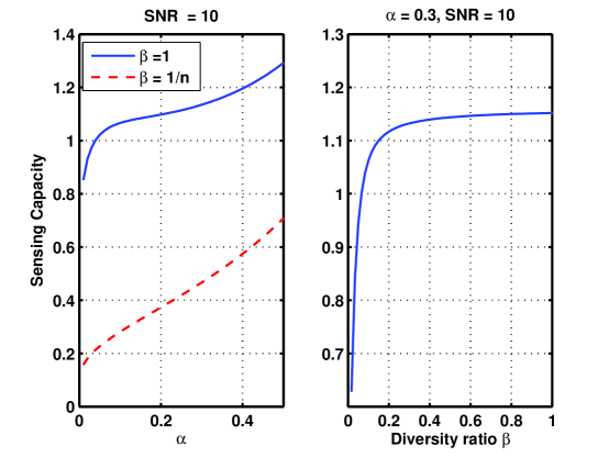
Figure 5: The gap between upper bounds to sensing capacity in very low diversity and full diversity for the binary alphabet case. Shown also is the Sensing Capacity as a function of diversity for fixed sparsity. Note the saturation effect with diversity ratio.

The effect is illustrated in figure 5. Thus low sensing diversity implies low sensing capacity.

VIII-B Effect of correlation in $\mathbf{G}$ on achievable sensing capacity

In this section we will show that correlation in sensing matrix $\mathbf{G}$ reduces achievable capacity. Correlation in $\mathbf{G}$ can arise due to many physical reasons such as correlated scattering, correlation of gains across modalities in sensing which may arise due to the physical construction of the sensor. Naturally there can be direct relations between various phenomena that can lead to such correlation. This is captured by assuming that there is correlation across the columns of $\mathbf{G}$. Consider the upper bound to the probability of error as derived in section IV,

$$Pr\left(\frac{1}{n}d(\mathbf{X},\hat{\mathbf{X}}(\mathbf{Y}))\geq 2d_{0}\right)\leq\exp\left\{-\min_{\mathbf{X}\in\mathcal{B}_{i},\mathbf{X}^{\prime}\in\mathcal{B}_{j}}\dfrac{SNR||\mathbf{G}(\mathbf{X}-\mathbf{X}^{\prime})||^{2}}{4}\right\}2^{n(R_{X}(d_{0})-K(n,d_{0}))}$$

In the above expression, the term

$$SNR||\mathbf{G}(\mathbf{X}-\mathbf{X}^{\prime})||^{2}=SNR\sum_{i=1}^{n}|\sum_{j=1}^{n}\mathbf{G}_{ij}(X_{i}-X^{\prime}_{j})|^{2}$$

where $\sum_{j=1}^{n}\mathbf{G}_{ij}(X_{i}-X^{\prime}_{j})$ for each $i$ are independent Gaussian random variables with zero mean and variance given by- $\Delta^{T}\Sigma_{\mathbf{G}_{i}}\Delta$ where $\Delta$ is the vector $\Delta=\mathbf{X}-\mathbf{X}^{\prime}$ and $\Sigma_{G_{i}}$ is the covariance matrix (symmetric and positive semi-definite) of the $i$-th row of $\mathbf{G}$. By construction, we know that $\frac{1}{n}\Delta^{T}\Delta\geq 2d_{0}$ and note that in the worst case,

$$\min\,\,\Delta^{T}\tilde{\Sigma}_{\mathbf{G}_{i}}\Delta=\lambda_{\min}\Delta^{T}\Delta$$

where $\lambda_{\min}$ is the minimum eigenvalue of the normalized covariance matrix $\tilde{\Sigma}_{\mathbf{G}_{i}}$. Proceeding in a manner similar to that in the proof of lemma VI.2 we have that,

$$Pr\left(\frac{1}{n}d(\mathbf{X},\hat{\mathbf{X}}(\mathbf{Y}))\geq 2d_{0}\right)\leq\left(\dfrac{1}{1+d_{0}SNR\lambda_{\min}}\right)^{m/2}2^{n(R_{X}(d_{0})-K(n,d_{0}))}$$

From the above expression one can see that achievable sensing capacity falls in general, since $\lambda_{min}\leq 1$ as compared to the case when the elements of $\mathbf{G}$ are uncorrelated in which case $\lambda_{\min}=1=\lambda_{\max}$.

VIII-C Deterministic $\mathbf{G}$

In this section we will consider deterministic matrices $\mathbf{G}$ and provide upper bounds to sensing capacity for the general case. To this end denote the rows of $\mathbf{G}$ as $\mathbf{G}_{i},\,i=1,\,2,\,\ldots,\,m$. Let the cross-correlations of these rows be denoted as:

$$r_{i}={\mathbf{G}_{i}^{T}\mathbf{G}_{i+1}\over\mathbf{G}_{i}^{T}\mathbf{G}_{i}}$$

As before to ensure the SNR, to be fixed we impose $\mathbf{G}_{i}^{T}\mathbf{G}_{i}=1$ for all $i$. Then we have the following result:

Lemma VIII.2

For the generative models for the signal $\mathbf{X}$ as outlined in the problem set-up, an upper bound for the sensing capacity for a deterministic sensing matrix $\mathbf{G}\in\mathbb{R}^{m\times n}$ is given by:

$$C(d_{0})\leq\sum_{i=1}^{m-1}{\log\left(1+SNR\alpha(1-r_{i})+{r_{i}\alpha SNR\over\alpha SNR+1}(1+\alpha SNR(1-r_{i}))\right)\over R_{X}(d_{0})-K(n,d_{0})}$$ (12)

Proof:

We will evaluate $I(\mathbf{X};\mathbf{Y}|\mathbf{G})$ via the straightforward method,

$$I(\mathbf{X};\mathbf{Y}|\mathbf{G})=h(\mathbf{Y}|\mathbf{G})-h(\mathbf{Y}|\mathbf{G},\mathbf{X})$$

Note that $h(\mathbf{Y}|\mathbf{G},\mathbf{X})=h(\mathbf{N})$. Note that $h(\mathbf{Y}|\mathbf{G})\leq h(\mathbf{Y})\leq h(\mathbf{Y}^{*})$ where $\mathbf{Y}^{*}$ is a Gaussian random vector obtained via $\mathbf{G}\mathbf{X}^{*}$ where $\mathbf{X}^{*}$ is now a Gaussian random vector with i.i.d components and with the same covariance as $\mathbf{X}$ under the generative model(s). We will now upper bound the entropy of $\mathbf{Y}$ via,

$$h(\mathbf{Y})\leq h(\mathbf{Y}^{*})\leq h(Y_{1}^{*})+\sum_{i=1}^{m-1}h(Y_{i+1}^{*}\mid Y_{i}^{*})\leq h(Y_{1}^{*})+h(Y_{i+1}^{*}-\eta_{i}Y_{i}^{*})$$

where $\eta_{i}Y_{i}^{*}$ is the best MMSE estimate for $Y_{i+1}^{*}$. The MMSE estimate of $Y_{i+1}^{*}$ from $Y_{i}^{*}$ is given by,

$$\hat{Y}_{i+1}^{*}=\frac{\Sigma_{Y_{i}^{*}Y_{i+1}^{*}}}{\Sigma_{Y_{i}^{*}}}Y_{i}^{*}$$

$\Sigma_{Y_{i}^{*}Y_{i+1}^{*}}=r_{i}\alpha SNR$ and $\Sigma_{Y_{i}^{*}}=\alpha SNR+1$. The result then follows by evaluating the MMSE error given by,

$$\mathbf{E}(Y_{i+1}^{*}-\hat{Y}_{i+1}^{*})^{2}=\mathbf{E}\left(Y_{i+1}^{*}-\frac{r_{i}\alpha SNR}{\alpha SNR+1}Y_{i}^{*}\right)^{2}$$

$$\begin{array}[]{ll}\mathbf{E}\left(Y_{i+1}^{*}-\frac{r_{i}\alpha SNR}{\alpha SNR+1}Y_{i}^{*}\right)^{2}&=\alpha SNR+1+\frac{(r_{i}\alpha SNR)^{2}}{\alpha SNR+1}-2\frac{(r_{i}\alpha SNR)^{2}}{\alpha SNR+1}\\ &=1+\alpha SNR(1-r_{i})+\frac{r_{i}\alpha SNR}{\alpha SNR+1}\left(1+(1-r_{i})\alpha SNR\right)\end{array}$$

Plugging in the quantities the result follows.

∎

Let us see the implications of the above result for one particular type of sensing matrix architecture induced via a random filtering and downsampling, considered in [20]. The output of the filter of length $L<n$ can be modeled via multiplication of $\mathbf{X}$ via a Toeplitz matrix (with a banded structure). The overlap between successive rows of the matrix $\mathbf{G}$ is $L-1$ in this case implying a large cross correlation $r_{i}$. From lemma 12 it follows that larger cross correlation in rows implies poor sensing capacity. Also note that for a filtering architecture one has to address a coverage issue wherein it is required that $m>n-L+1$. This implies that $L>n-m+1$. Thus the filter length has to be sufficiently large which implies that cross-correlation is also large.

Indeed randomizing each row will lead to low cross-correlation (in an expected sense) but the coverage issue still needs to be addressed. On the other hand one can subsample the output signal of length $n-L+1$ by some factor so as to reduce the cross correlation yet ensuring coverage. In this case the matrix almost becomes like a upper triangular matrix and there is a significant loss of sensing diversity. A loose tradeoff between the filter-length $L$ and the sampling factor $d$ (say) immediately follows from lemma 12 where the cross correlation changes according to $r_{i}=\dfrac{L(1-d)}{n}$

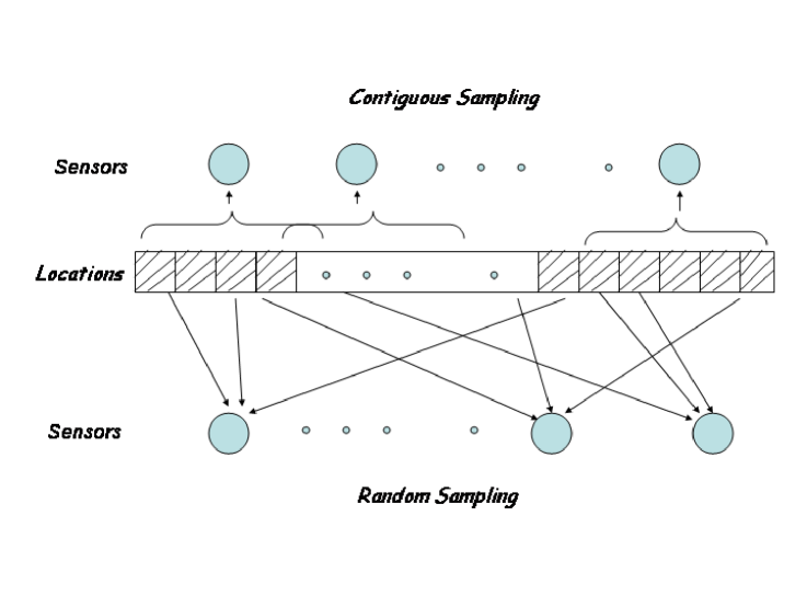
Figure 6: Illustration of random sampling Vs contiguous sampling in a sensor network. This leads to different structures on the sensing matrix and that leads to different performance.

IX Upper bounds on Sensing Capacity for $\left\{0,1\right\}$ ensemble

The main motivation for considering this ensemble comes from scenarios where randomization in the elements of $\mathbf{G}$ is not feasible, e.g. field estimation from smoothed data. In this case each sensor measures a superposition of the signals that are in the sensing range of the sensor. This leads us to consider other types of modalities, e.g. contiguous sampling of $\mathbf{X}$ by each sensor Vs random sampling for $\beta<1$. An illustration of the two types of sampling is shown in figure 6. We reveal the following contrast for the two cases for same $\beta<1$

Lemma IX.1

Random Sampling: For the $\left\{0,1\right\}$ ensemble for sensing matrices consider the case when each row of $\mathbf{G}$ has $\beta n$ ones randomly placed in $n$ positions. Then for discrete $\mathbf{X}\in\left\{0,1\right\}^{n}$ drawn Bernoulli$(\alpha)$ and for $d_{0}<\alpha$,

$$C_{rand}(d_{0})\leq\frac{H(J)}{h_{2}(\alpha)-h_{2}(d_{0})}$$

where $H(.)$ is the discrete entropy function and where $J$ is a random variable with distribution given by

$$\Pr(J=j)=\dfrac{\binom{\alpha n}{j}\binom{n(1-\alpha)}{\beta n-j}}{\binom{n}{\beta n}}$$

Proof:

See Appendix. ∎

Lemma IX.2

Contiguous Sampling: For the $\left\{0,1\right\}$ ensemble for sensing matrices consider the case where each row of $\mathbf{G}$ has $\beta n$ consecutive ones randomly placed with wrap around. Then for discrete $\mathbf{X}\in\left\{0,1\right\}^{n}$ drawn Bernoulli$(\alpha)$ and $d_{0}<\alpha$,

$$C_{contg.}(d_{0})\leq\frac{h_{2}(\alpha+\beta)}{h_{2}(\alpha)-h_{2}(d_{0})}$$

Proof:

See Appendix. ∎

As seen the upper bound, $C_{rand}(d_{0})\geq C_{contg.}(d_{0})$. Thus randomization in $\mathbf{G}$ performs better. The difference is shown in figure 7 for a low sparsity scenario. The proofs of the lemmas IX.1 and IX.2 follow from the upper bounds to the mutual information terms as provided in section XII and then applying the necessary conditions for the lower bound on the probability of error to be lower bounded by zero.

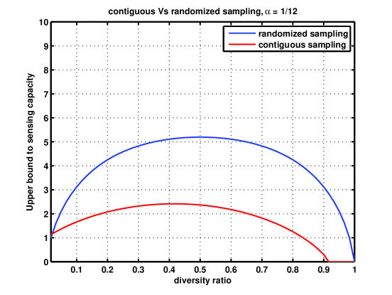
Figure 7: A comparison of the upper bounds to sensing capacity for the randomized sampling Vs contiguous sampling case. $\mathbf{X}$ is the Bernoulli model and the ensemble for $\mathbf{G}$ is the $\left\{0,1\right\}$ ensemble. We have selected the case of low sparsity in this case. Note that due to loose overbounding of mutual information (we basically got rid of noise) the upper bounds are greater than in the case of Gaussian ensemble.

X Estimation of functions of $\mathbf{X}$

The analysis of lower bounds to the probability of error presented in this paper extend in a straightforward way to estimation of functions of $\mathbf{X}$. In this section we will consider one such scenario that has received attention in relation to problems arising in physics. The discussion below will reveal the power of the method presented in this work and it is easily capable of handling more complicated cases and scenarios, though the computation of the terms involved in the analysis may become hard.

X-A Detecting the sign pattern of $\mathbf{X}$

Of particular interest is to estimate the sign pattern of the underlying signal $\mathbf{X}$. To this end define a new random variable $\mathbf{U}$, via

$$U_{i}=\left\{\begin{array}[]{ll}1&\mbox{if}\,\,X_{i}>0\\ -1&\mbox{if}\,\,X_{i}<0\\ 0&\mbox{if}\,\,X_{i}=0\end{array}\right.$$

The corresponding $n$ dimensional extension and probability distribution on $\mathbf{U}$ is induced directly via $P_{\mathbf{X}}$. In such a case note that $\mathbf{U}\rightarrow\mathbf{X}\rightarrow\mathbf{Y}\rightarrow\hat{\mathbf{U}}(\mathbf{Y})$ forms a Markov chain. To this end consider an error event defined via,

$$E=\left\{\begin{array}[]{ll}1&\mbox{if}\,\,\mathbf{U}\neq\hat{\mathbf{U}}(\mathbf{Y})\\ 0&\mbox{otherwise}\end{array}\right.$$

Then we have,

$$\begin{array}[]{lll}H(\mathbf{U},E|\mathbf{Y})&=&\underset{\leq 1}{\underbrace{H(E|\mathbf{Y})}}+H(\mathbf{U}|E,\mathbf{Y})\\ &=&H(\mathbf{U}|\mathbf{Y})+\underset{=0}{\underbrace{H(E|\mathbf{U},\mathbf{Y})}}\end{array}$$

Thus we have

$$H(\mathbf{U}|\mathbf{Y})\leq 1+P_{e}\underset{\leq n\log 3}{\underbrace{H(\mathbf{U}|E=1,\mathbf{Y})}}+\underset{=0}{\underbrace{(1-P_{e})H(\mathbf{U}|E=0,\mathbf{Y})}}$$

This implies,

$$P_{e}\geq\frac{H(\mathbf{U})-I(\mathbf{U};\mathbf{Y}|\mathbf{G})-1}{n\log 3}$$

In order to evaluate the $I(\mathbf{U};\mathbf{Y}|\mathbf{G})$ we note that $I(\mathbf{U},\mathbf{X};\mathbf{Y}|\mathbf{G})=I(\mathbf{X};\mathbf{Y}|\mathbf{G})$. This follows from , $I(\mathbf{U},\mathbf{X};\mathbf{Y}|\mathbf{G})=H(\mathbf{U},\mathbf{X})-H(\mathbf{X},\mathbf{U}|\mathbf{Y},\mathbf{G})=H(\mathbf{X})-H(\mathbf{X}|\mathbf{G},\mathbf{Y})-H(\mathbf{U}|\mathbf{G},\mathbf{Y},\mathbf{X})=I(\mathbf{X};\mathbf{Y}|\mathbf{G})$. Thus $I(\mathbf{U};\mathbf{Y}|\mathbf{G})=I(\mathbf{X};\mathbf{Y}|\mathbf{G})-I(\mathbf{X};\mathbf{Y}|\mathbf{G},\mathbf{U})$ and both these terms can be adequately bounded/evaluated.

XI Appendix

XI-A Proof of lemma III.1

Let $X^{n}=\left\{X_{1},...,X_{n}\right\}$ be an i.i.d. sequence where each variable $X_{i}$ is distributed according to a distribution $P_{X}$ defined on the alphabet ${\cal X}$. Denote $P_{X^{n}}\triangleq(P_{X})^{n}$ the n-dimensional distribution induced by $P_{X}$. Let the space ${\cal X}^{n}$ be equipped with a distance measure $d(.,.)$ with the distance in $n$ dimensions given by $d_{n}(X^{n},Z^{n})=\sum_{k=1}^{n}d(X_{k},Z_{k})$ for $X^{n},Z^{n}\in{\cal X}^{n}$. Given $\epsilon>0$, there exist a set of points $\left\{Z_{1}^{n},...,Z_{N_{\epsilon}(n,d_{0})}\right\}\subset{\cal X}^{n}$ such that,

$$P_{X^{n}}\left(\bigcup_{i=1}^{N_{\epsilon}(n,d_{0})}{\cal B}_{i}\right)\geq 1-\epsilon$$ (13)

where ${\cal B}_{i}\triangleq\left\{X^{n}:\frac{1}{n}d_{n}(X^{n},Z_{i}^{n})\leq d_{0}\right\}$, i.e., the $d_{0}$ balls around the set of points cover the space ${\cal X}^{n}$ in probability exceeding $1-\epsilon$.

Given such set of points there exists a function $f(X^{n}):X^{n}\rightarrow Z_{i}^{n}\,\,s.t.\,\,Pr\left(\frac{1}{n}d_{n}(X^{n},Z_{i}^{n})\leq d_{0}\right)\geq 1-\epsilon$. To this end, let $T_{P_{{X}^{n}}}$ denote the set of $\delta$ - typical sequences in ${\cal X}^{n}$ that are typical $P_{X^{n}}$, i.e.

$$T_{P_{{X}^{n}}}=\left\{X^{n}:|-\frac{1}{n}\log\hat{P}(X^{n})-H(X)|\leq\delta\right\}$$

where $\hat{P}(X^{n})$ is the empirical distribution induced by the sequence $X^{n}$. We have the following lemma from [21].

Lemma XI.1

For any $\eta>0$ there exists an $n_{0}$ such that for all $n\geq n_{0}$, such that

$$Pr\left(X^{n}:|-\frac{1}{n}\log\hat{P}(X^{n})-H(X)|<\delta\right)>1-\eta$$

In the following we choose $\eta=\delta$. Given that there is an algorithm $\hat{X}^{n}(\mathbf{Y})$ that produces an estimate of $X^{n}$ given the observation $\mathbf{Y}$. To this end define an error event on the algorithm as follows,

$$E_{n}=\left\{\begin{array}[]{l}1\,\,\mbox{if}\,\,\,\frac{1}{n}d_{n}(X^{n},\hat{X}^{n}(\mathbf{Y}))\geq d_{0}\\ 0\,\,\mbox{otherwise}\end{array}\right.$$

Define another event $A_{n}$ as follows

$$A_{n}=\left\{\begin{array}[]{l}1\,\,\mbox{if}\,\,\,X^{n}\in T_{P_{X^{n}}}\\ 0\,\,\mbox{otherwise}\end{array}\right.$$

Note that since $X^{n}$ is drawn according to $P_{X^{n}}$ and given $\delta>0$ we choose $n_{0}$ such that conditions of lemma XI.1 are satisfied. In the following we choose $n\geq n_{0}(\delta)$. Then a priori, $Pr(A_{n}=1)\geq(1-\delta)$. Now, consider the following expansion,

$$\begin{array}[]{l}H(f(X^{n}),E_{n},A_{n}|\mathbf{Y})\\ =H(f(X^{n})|\mathbf{Y})+H(E_{n},A_{n}|f(X^{n}),\mathbf{Y})\\ =H(E_{n},A_{n}|\mathbf{Y})+H(f(X^{n})|E_{n},A_{n},\mathbf{Y})\end{array}$$

This implies that

$$\begin{array}[]{l}H(f(X^{n})|\mathbf{Y})\\ =H(E_{n},A_{n}|\mathbf{Y})-H(E_{n},A_{n}|f(X^{n}),\mathbf{Y})+H(f(X^{n})|E_{n},A_{n},\mathbf{Y})\\ =I(E_{n},A_{n};f(X^{n})|\mathbf{Y})+H(f(X^{n})|E_{n},A_{n},\mathbf{Y})\\ \leq H(E_{n},A_{n})+H(f(X^{n})|E_{n},A_{n},\mathbf{Y})\\ \leq H(E_{n})+H(A_{n})+H(f(X^{n})|E_{n},A_{n},\mathbf{Y})\end{array}$$

Note that $H(E_{n})\leq 1$ and $H(A_{n})=\delta\log\frac{1}{\delta}+(1-\delta)\log\frac{1}{1-\delta}\sim\delta$. Thus we have

$$\begin{array}[]{ll}&H(f(X^{n})|\mathbf{Y})\leq 1+\delta+P_{e}^{n}H(f(X^{n})|\mathbf{Y},E_{n}=1,A_{n})\\ &+(1-P_{e}^{n})H(f(X^{n})|\mathbf{Y},E_{n}=0,A_{n})\end{array}$$

Now the term $P_{e}^{n}H(f(X^{n})|\mathbf{Y},E_{n}=1,A_{n})\leq P_{e}^{n}\log N_{\epsilon}(n,d_{0})$. Note that the second term does not go to zero. For the second term we have that,

$$\begin{array}[]{l}(1-P_{e}^{n})H(f(X^{n})|\mathbf{Y},E_{n}=0,A_{n})\\ =P(A_{n}=1)(1-P_{e}^{n})H(f(X^{n})|\mathbf{Y},E_{n}=0,A_{n}=1)\\ \hskip 14.22636pt+P(A_{n}=0)(1-P_{e}^{n})H(f(X^{n})|\mathbf{Y},E_{n}=0,A_{n}=0)\\ \leq(1-P_{e}^{n})H(f(X^{n})|\mathbf{Y},E_{n}=0,A_{n}=1)\\ \hskip 14.22636pt+\delta(1-P_{e}^{n})\log\left(N_{\epsilon}(n,d_{0})\right)\end{array}$$

The first term on R.H.S in the above inequality is bounded via,

$$(1-P_{e}^{n})H(f(X^{n})|\mathbf{Y},E_{n}=0,A_{n}=1)\leq(1-P_{e}^{n})\log\left(|{\cal S}|\right)$$

where ${\cal S}$ is the set given by,

$${\cal S}=\left\{i:d_{set}\left({{\cal B}_{f(X^{n})},\cal B}_{i}\right)\leq d_{0}\right\}$$

where $d_{set}(S_{1},S_{2})=\min_{s\in S_{1},s^{\prime}\in S_{2}}d_{n}(s,s^{\prime})$ is the set distance between two sets. Now note that $I(f(X^{n});X^{n})=H(f(X^{n}))$ and $H(f(X^{n})|\mathbf{Y})=H(f(X^{n}))-I(f(X^{n});X^{n})\geq H(f(X^{n}))-I(X^{n};\mathbf{Y})$ where the second inequality follows from data processing inequality over the Markov chain $f(X^{n})\leftrightarrow X^{n}\leftrightarrow\mathbf{Y}$. Thus we have,

$$\begin{array}[]{ll}P_{e}^{n}\geq&\dfrac{I(f(X^{n});X^{n})-\log|{\cal S}|-I(X^{n};\mathbf{Y})-1}{(1-\delta)\log N_{\epsilon}(n,d_{0})-\log|{\cal S}|}\\ \\ &-\dfrac{\delta(1+\log N_{\epsilon}(n,d_{0}))}{(1-\delta)\log N_{\epsilon}(n,d_{0})-\log|{\cal S}|}\end{array}$$

The above inequality is true for all the mappings $f$ satisfying the distortion criteria for mapping $X^{n}$ and for all choices of the set satisfying the covering condition given by XI.2. We now state the following lemma for a minimal covering, taken from [16].

Lemma XI.2

Given $\epsilon>0$ and the distortion measure $d_{n}(.,.)$, let $N_{\epsilon}(n,d_{0})$ be the minimal number of points $Z_{1}^{n},...,Z_{N_{\epsilon}(n,d_{0})}^{n}\subset{\cal X}^{n}$ satisfying the covering condition,

$$P_{X^{n}}\left(\bigcup_{i=1}^{N_{\epsilon}(n,d_{0})}{\cal B}_{i}\right)\geq 1-\epsilon$$

Let $N_{\epsilon}(n,d_{0})$ be the minimal such number. Then,

$$\limsup_{n}\frac{1}{n}N_{\epsilon}(n,d_{0})=R_{X}(\epsilon,d_{0})$$

where $R_{X}(\epsilon,d_{0})$ is the infimum of the $\epsilon$- achievable rates at distortion level $d_{0}$.

Note that $\lim_{\epsilon\downarrow 0}R_{X}(\epsilon,d_{0})=R_{X}(d_{0})$ where $R_{X}(d_{0})=\min_{p(\hat{X}|X)}I(\hat{X};X)\,\,\,\mbox{subject to}\,\,\frac{1}{n}E(d(X^{n},\hat{X}^{n}))\leq d_{0}$. In order to lower bound $P_{e}^{n}$ we choose the mapping $f(X^{n})$ to correspond to the minimal cover. Also w.l.o.g we choose $\delta=\epsilon$. We note the following.

1. From lemma XI.1, given $\epsilon>0$, $\exists n_{0}(\epsilon)$ such that for all $n\geq n_{0}(\epsilon)$, we have $Pr(T_{P_{X^{n}}})\geq 1-\epsilon$.

2. Given $\epsilon>0$ and for all $\beta>0$, for the minimal cover we have from lemma XI.2 that $\exists\,n_{1}(\beta)$ such that for all $n\geq n_{1}(\beta)$, $N_{\epsilon}(n,d_{0})\leq n(R_{X}(\epsilon,d_{0})+\beta)$.

3. From the definition of the rate distortion function we have for the choice of the functions $f(X^{n})$ that satisfies the distortion criteria, $I(f(X^{n});X^{n})\geq nR_{X}(\epsilon,d_{0})$.

Therefore we have for $n\geq\max(n_{0},n_{1})$,

$$\begin{array}[]{ll}P_{e}^{n}\geq&\dfrac{nR_{X}(\epsilon,d_{0})-\log|{\cal S}|-I(X^{n};\mathbf{Y})-1}{(1-\epsilon)(n(R_{X}(\epsilon,d_{0})+\beta)-\log|{\cal S}|}\\ \\ &-\dfrac{\epsilon(1+n(R_{X}(\epsilon,d_{0})+\beta)}{(1-\epsilon)n(R_{X}(\epsilon,d_{0})+\beta)-\log|{\cal S}|}\end{array}$$

Clearly, $\log|S|\leq\frac{n}{2}R_{X}(\epsilon,d_{0})$.

Limiting case

Since the choice of $\epsilon,\beta$ is arbitrary we can choose them to be arbitrary small. In fact we can choose $\epsilon,\beta\downarrow 0$. Also note that for every $\epsilon>0$ and $\beta>0$ there exists $n_{2}(\beta)$ such that $R_{X}(d_{0})+\beta\geq R_{X}(\epsilon,d_{0})\geq R_{X}(d_{0})-\beta$. Therefore for all $n\geq\max(n_{0},n_{1},n_{2})$ in the limiting case when $\epsilon,\beta\downarrow 0$, we have

$$P_{e}\geq\frac{R_{X}(d_{0})-\frac{1}{n}\log|{\cal S}|-\frac{1}{n}I(X^{n};\mathbf{Y})}{R_{X}(d_{0})-\frac{1}{n}\log|{\cal S}|}-o(1)$$

This implies that

$$P_{e}\geq\frac{R_{X}(d_{0})-\frac{1}{n}\log|{\cal S}|-\frac{1}{n}I(X^{n};\mathbf{Y})}{R_{X}(d_{0})}-o(1)$$

The proof then follows by identifying $K(n,d_{0})=\frac{1}{n}\log|{\cal S}|$, and is bounded above by a constant.

XI-B Proof of lemma III.2

Proof:

Given an observation $\mathbf{Y}$ about the event $X^{n}$. Define an error event,

$$E=\left\{\begin{array}[]{l}1\,\,\mbox{if}\,\,\,\frac{1}{n}d_{H}(X^{n},\hat{X}^{n}(\mathbf{Y}))\geq d_{0}\\ 0\,\,\mbox{otherwise}\end{array}\right.$$

Expanding $H(X^{n},E|\mathbf{Y})$ in two different ways we get that,

$$H(X^{n}|\mathbf{Y})\leq 1+nP_{e}\log(|{\cal X}|)+(1-P_{e})H(X^{n}|E=0,\mathbf{Y})$$

Now the term

$$\begin{array}[]{l}(1-P_{e})H(X^{n}|E=0,\mathbf{Y})\\ \leq(1-P_{e})\binom{n}{d_{0}n}(|{\cal X}|-1)^{nd_{0}}\\ \leq n(1-P_{e})\left(h(d_{0})+d_{0}\log(|{\cal X}|-1)\right)\end{array}$$

Then we have for the lower bound on the probability of error that,

$$P_{e}\geq\frac{H(X^{n}|\mathbf{Y})-n\left(h(d_{0})+d_{0}\log(|{\cal X}|-1)\right))-1}{n\log(|{\cal X}|)-n\left(h(d_{0})+d_{0}\log(|{\cal X}|-1)\right)}$$

Since $H(X^{n}|\mathbf{Y})=H(X^{n})-I(X^{n};\mathbf{Y})$ we have

$$P_{e}\geq\frac{n\left(H(X)-h(d_{0})-d_{0}\log(|{\cal X}|-1)\right)-I(X^{n};\mathbf{Y})-1}{n\log(|{\cal X}|)-n\left(h(d_{0})+d_{0}\log(|{\cal X}|-1)\right)}$$

It is known that $R_{X}(d_{0})\geq H(X)-h(d_{0})-d_{0}\log(|{\cal X}|-1)$, with equality iff

$$d_{0}\leq(|{\cal X}|-1)\min_{X\in{\cal X}}P_{X}$$

see e.g., [16]. Thus for those values of distortion we have for all $n$,

$$P_{e}\geq\frac{nR_{X}(d_{0})-I(X^{n};\mathbf{Y})-1}{n\log(|{\cal X}|)-n\left(h(d_{0})+d_{0}\log(|{\cal X}|-1)\right)}$$

∎

XI-C Rate distortion function for the mixture Gaussian source under squared distortion measure

It has been shown in [22] that the rate distortion function for a mixture of two Gaussian sources with variances given by $\sigma_{1}$ with mixture ratio $\alpha$ and $\sigma_{0}$ with mixture ratio $1-\alpha$, is given by

$$\begin{array}[]{l}R_{mix}(D)=\\ \left\{\begin{array}[]{l}H(\alpha)+\frac{(1-\alpha)}{2}\log(\frac{\sigma_{0}^{2}}{D})+\frac{\alpha}{2}\log(\frac{\sigma_{1}^{2}}{D})\,\,\mbox{if}\,\,D<\sigma_{0}^{2}\\ H(\alpha)+\frac{\alpha}{2}\log(\frac{\alpha\sigma_{1}^{2}}{D-(1-\alpha)\sigma_{0}^{2}})\,\,\mbox{if}\,\,\sigma_{0}^{2}<D\leq(1-\alpha)\sigma_{0}^{2}+\alpha\sigma_{1}^{2}\end{array}\right.\end{array}$$

For a strict sparsity model we have $\sigma_{0}^{2}\rightarrow 0$ we have that,

$$R_{mix}(D)=\begin{array}[]{l}H(\alpha)+\frac{\alpha}{2}\log(\frac{\alpha\sigma_{1}^{2}}{D})\,\,\mbox{if}\,\,0<D\leq\alpha\sigma_{1}^{2}\end{array}$$

XI-D Bounds on Mutual information

In this section we will evaluate bounds on mutual information that will be useful in characterization of the Sensing Capacity. Given that the matrix $\mathbf{G}$ is chosen independently of $\mathbf{X}$ we expand the mutual information between $\mathbf{X}$ and $\mathbf{Y},\mathbf{G}$ in two different ways as follows –

$$\begin{array}[]{ll}I(\mathbf{X};\mathbf{Y},\mathbf{G})&=\underset{=0}{\underbrace{I(\mathbf{X};\mathbf{G})}}+I(\mathbf{X};\mathbf{Y}|\mathbf{G})\\ &=I(\mathbf{X};\mathbf{Y})+I(\mathbf{X};\mathbf{G}|\mathbf{Y})\end{array}$$

This way of expanding gives us handle onto evaluating the mutual information with respect to the structure of the resulting sensing matrix $\mathbf{G}$. From above we get that,

$$\begin{array}[]{ll}I(\mathbf{X};\mathbf{Y}|\mathbf{G})&=I(\mathbf{X};\mathbf{Y})+I(\mathbf{X};\mathbf{G}|\mathbf{Y})\\ &=h(\mathbf{Y})-h(\mathbf{Y}|\mathbf{X})+h(\mathbf{G}|\mathbf{Y})-h(\mathbf{G}|\mathbf{X},\mathbf{Y})\end{array}$$

To this end we have the following lemma.

Lemma XI.3

For a sparsity level of $\alpha$ and diversity factor of $\beta=1$,

$$I(\mathbf{X};\mathbf{Y}|\mathbf{G})\leq\frac{m}{2}\log(1+\frac{\alpha P}{N_{0}})$$

Proof:

First note that,

$$h(\mathbf{Y})\leq\frac{m}{2}\log 2\pi e(N_{0}+\alpha P)$$

Since conditioned on $\mathbf{X}$, $\mathbf{Y}$ is distributed with a Gaussian density we have,

$$h(\mathbf{Y}|\mathbf{X})=\frac{m}{2}\log 2\pi e\left(N_{0}+\frac{\sum_{i=1}^{k}\mathbf{X}_{i}^{2}P}{n}\right)$$

$$h(\mathbf{G}|\mathbf{Y})\leq h(\mathbf{G})=\frac{mn}{2}\log\left(2\pi e\frac{P}{n}\right)$$

Note also that conditioned on $\mathbf{X}$ and $\mathbf{Y}$ the $\mathbf{G}$ has a Gaussian distribution. Now note that, $h(\mathbf{G}|\mathbf{Y},\mathbf{X})$. First note that, rows of $\mathbf{G}$ are independent of each other given $\mathbf{X}$ and $\mathbf{Y}$. So we can write,

$$h(\mathbf{G}|\mathbf{Y},\mathbf{X})=mh(\mathbf{g_{1}}|\mathbf{Y},\mathbf{X})$$

where $\mathbf{g}_{1}$ is the first row of the matrix $\mathbf{G}$. Since $\mathbf{g}$ is Gaussian one can find the residual entropy in terms of the residual MMSE error in estimation of $\mathbf{g}$ given $\mathbf{X}$ and $\mathbf{Y}$. This error is given by –

$$\begin{array}[]{ll}\mbox{MMSE}_{\mathbf{g}_{1}|\mathbf{Y},\mathbf{X}}&=\Sigma_{\mathbf{g}_{1}|\mathbf{X}}-\Sigma_{\mathbf{g}_{1}\mathbf{Y}|\mathbf{X}}\Sigma_{\mathbf{Y}|\mathbf{X}}^{-1}\Sigma_{\mathbf{g}_{1}\mathbf{Y}|\mathbf{X}}^{T}\\ &=\Sigma_{\mathbf{g}_{1}}-\Sigma_{\mathbf{g}_{1}\mathbf{Y}_{1}|\mathbf{X}}\Sigma_{\mathbf{Y}_{1}|\mathbf{X}}^{-1}\Sigma_{\mathbf{g}_{1}\mathbf{Y}_{1}|\mathbf{X}}^{T}\end{array}$$

The second equation follows from the fact that $\mathbf{G}$ is independent of $\mathbf{X}$ and given $\mathbf{X}$ the row $\mathbf{g}_{1}$ is independent of other observations, $\mathbf{Y}_{2},...,\mathbf{Y}_{m}$. First note that given $\mathbf{X}$ we also know which positions of $\mathbf{X}$ are zeros. So without lossof generality we can assume that the first $k$ elements of $\mathbf{X}$ are non-zeros and the rest are zeros. Now note the following,

$$\Sigma_{\mathbf{g}_{1}}=\frac{P}{n}I_{n}$$

$$\Sigma_{\mathbf{g}_{1}\mathbf{Y}_{1}|\mathbf{X}}=\frac{P}{n}\begin{pmatrix}\mathbf{X}_{1}\\ \vdots\\ \mathbf{X}_{k}\\ \mathbf{0}_{n-k}\end{pmatrix}$$

where $\mathbf{0}_{n-k}$ is a column vector of $n-k$ zeros.

$$\Sigma_{\mathbf{Y}_{1}|\mathbf{X}}=\frac{P}{n}\sum_{i=1}^{k}\mathbf{X}_{i}^{2}+N_{0}$$

Therefore we have,

$$\begin{array}[]{l}h(\mathbf{g}_{1}|\mathbf{Y}_{1},\mathbf{X})\\ =\frac{1}{2}\log(2\pi e)^{k}\det\left(\frac{P}{n}I_{k}-\frac{P}{n}\mathbf{X}_{1:k}\Sigma_{\mathbf{Y}_{1}|\mathbf{X}}^{-1}\frac{P}{n}\mathbf{X}_{1:k}^{T}\right)\\ +\frac{n-k}{2}\log 2\pi e\frac{P}{n}\end{array}$$

Note that the second term on the R.H.S in the above equation corresponds to the entropy of those elements of the row $\mathbf{g}_{1}$ that have no correlation with $\mathbf{Y}$, i.e. nothing can be inferred about these elements since they overlap with zero elements of $\mathbf{X}$. Now, using the equation $\det(I+AB)=\det(I+BA)$, we have that

$$\begin{array}[]{ll}h(\mathbf{g}_{1}|\mathbf{Y}_{1},\mathbf{X})&=\frac{1}{2}\log(\frac{2\pi eP}{n})^{k}\det\left(1-\mathbf{X}_{1:k}^{T}\Sigma_{\mathbf{Y}_{1}|\mathbf{X}}^{-1}\frac{P}{n}\mathbf{X}_{1:k}\right)\\ &=\frac{1}{2}\log\left((\frac{2\pi eP}{n})^{k}\frac{N_{0}}{\frac{P}{n}\sum_{i=1}^{k}\mathbf{X}_{i}^{2}+N_{0}}\right)\end{array}$$

Plugging in all the expressions we get a lower bound on the mutual information $I(\mathbf{X};\mathbf{Y}|\mathbf{G})$ -

$$I(\mathbf{X};\mathbf{Y}|\mathbf{G})\leq\frac{m}{2}\log(1+\frac{\alpha P}{N_{0}})$$

∎

In contrast to the upper bound derived in the proof of lemmas V.1 and V.2, this alternate derivation provides a handle to understand the effect of the structure of $\mathbf{G}$ on the mutual information when one is not allowed to pick a maximizing input distribution on $\mathbf{X}$. Moreover the above derivation can potentially handle scenarios of correlated $\mathbf{G}$. Below we will use the above result in order to prove lemma VIII.1.

XI-E Proof of lemma VIII.1

To this end let $l=\beta n$ and is fixed, i.e. there are only $l$ non-zero terms in each row of matrix $\mathbf{G}$. We have

$$h(\mathbf{G})=\frac{ml}{2}\log 2\pi e\frac{P}{l}+mh_{2}(\beta)$$

Now we will first evaluate $h(\mathbf{G}|\mathbf{Y},\mathbf{X})$. Proceeding as in derivation of lemma XI.3, we have that,

$$h(\mathbf{G}|\mathbf{X},\mathbf{Y})=mh(\mathbf{g}_{1}|\mathbf{Y}_{1},\mathbf{X})+mh_{2}(\beta)$$

where one can see that if the matrix $\mathbf{G}$ is chosen from a Gaussian ensemble then given $\mathbf{X}$ and $\mathbf{Y}$ it tells nothing about the positions of the non-zeros in each row. Hence the additive term $h_{2}(\beta)$ appears in both terms and is thus canceled in the overall calculations. So we will omit this term in the subsequent calculations. To this end, let $j$ denote the number of overlaps of the vector $\mathbf{g}_{1}$ and the k-sparse vector $\mathbf{X}$. Given $\mathbf{Y}_{1}$ and $\mathbf{X}$ one can only infer something about those elements of $\mathbf{G}$ that contribute to $\mathbf{Y}_{1}$. Given the number of overlaps $j$ we then have

$$\begin{array}[]{l}h(\mathbf{g}_{1}|\mathbf{X},\mathbf{Y}_{1},j)=\frac{l-j}{2}\log 2\pi e\frac{P}{l}+\frac{1}{2}\log\left((\frac{2\pi eP}{l})^{j}\frac{N_{0}}{\frac{P}{l}\sum_{i=1}^{j}\mathbf{X}_{j}^{2}+N_{0}}\right)\end{array}$$

where we have assumed without loss of generality that the first $j$ elements of $\mathbf{X}$ are non-zero and overlap with elements of the first row. Now note that,

$$h(\mathbf{Y}|j)\leq\frac{m}{2}\log 2\pi e(\frac{Pj}{l}+N_{0})$$

$$h(\mathbf{Y}|\mathbf{X},j)=\frac{m}{2}\log 2\pi e\left(\frac{P}{l}\sum_{i=1}^{j}\mathbf{X}_{i}^{2}+N_{0}\right)$$

From above we have that,

$$I(\mathbf{X};\mathbf{Y}|\mathbf{G},j)=\frac{m}{2}\log(1+\frac{jP}{lN_{0}})$$

Taking the expectation with respect to the variable $j$ we have,

$$I(\mathbf{X};\mathbf{Y}|\mathbf{G})=\frac{m}{2}\mathbf{E}_{j}\log(1+\frac{jP}{lN_{0}})$$

Note that $j\leq\min\left\{k,l\right\}$ and has a distribution given by,

$$\Pr(j)=\dfrac{\binom{k}{j}\binom{n-k}{l-j}}{\binom{n}{l}}$$

XII Upper bounds to Mutual information for $\left\{0,1\right\}$ ensemble

In this section we will derive upper bounds to the mutual information $I(\mathbf{X};\mathbf{Y}|\mathbf{G})$ for the case when the matrix is chosen from a $\left\{0,1\right\}$ ensemble. First it is easily seen that for this ensemble a full diversity leads to loss of rank and thus the mutual information is close to zero. So we will only consider the case $\beta<1$.

XII-A Random locations of $1$’s in $\mathbf{G}$

In this section we will provide simple upper bounds to the mutual information $I(\mathbf{X};\mathbf{Y}|\mathbf{G})$ for the case of $\left\{0,1\right\}$ ensemble of sensing matrices. Note that,

$$I(\mathbf{X};\mathbf{Y}|\mathbf{G})\leq I(\mathbf{X};\mathbf{G}\mathbf{X}|\mathbf{G})$$

Let $\tilde{\mathbf{Y}}=\mathbf{G}\mathbf{X}$. Then we have,

$$I(\mathbf{X};\tilde{\mathbf{Y}}|\mathbf{G})=I(\mathbf{X};\tilde{\mathbf{Y}})+I(\mathbf{X};\mathbf{G}|\tilde{\mathbf{Y}})$$

Now note that $\frac{1}{n}I(\mathbf{X};\tilde{\mathbf{Y}})=o(1)$. Then we need to evaluate $I(\mathbf{G};\mathbf{X}|\tilde{\mathbf{Y}})\leq H(\mathbf{G})-H(\mathbf{G}|\tilde{\mathbf{Y}},\mathbf{X})$. Now note that since each row of $\mathbf{G}$ is an independent Bernoulli$\sim\beta$ sequence we can split the entropy into sum of entropies each individual rows. To this end focus on the first row. Then conditioned on there being $l$ $1$’s in the row we have,

$H(\mathbf{G}_{1}|l)\leq\binom{n}{l}$. Given that $X$ is $k$-sparse we have,

$$H(\mathbf{G}_{1}|\mathbf{X},\tilde{\mathbf{Y}},l,k)=\sum_{j=0}^{\min(k,l)}\dfrac{\binom{k}{j}\binom{n-k}{l-j}}{\binom{n}{l}}\log\binom{k}{j}\binom{n-k}{l-j}$$

Thus we have

$$I(\mathbf{X};\mathbf{G}|\tilde{\mathbf{Y}},k,l)\leq\binom{n}{l}-\sum_{j=0}^{\min(k,l)}\dfrac{\binom{k}{j}\binom{n-k}{l-j}}{\binom{n}{l}}\log\binom{k}{j}\binom{n-k}{l-j}=H(J|k,l)$$

where $J$ is a random variable with distribution given by,

$$Pr(J=j)=\dfrac{\binom{k}{j}\binom{n-k}{l-j}}{\binom{n}{l}}$$

For large enough $n$, $k=\alpha n$ and $l=\beta n$ w.h.p. Thus $I(\mathbf{X};\mathbf{G}|\mathbf{Y})\leq H(\tilde{J})$, where $\tilde{J}$ has a limiting distribution given by,

$$Pr(\tilde{J}=j)=\dfrac{\binom{\alpha n}{j}\binom{n(1-\alpha)}{\beta n-j}}{\binom{n}{\beta n}}$$

In other words given $\epsilon>0$ there exists an $n_{0}$ such that for all $n\geq n_{0}$, $\underset{j}{\sup}|P_{J}(j)-P_{\tilde{J}}(j)|\leq\epsilon$ and by continuity of the entropy function, [[16], pp. 33, Lemma 2.7], it follows that $|H(J)-H(\tilde{J})|\leq-\epsilon\log\dfrac{\epsilon}{n}$

XII-B Contiguous sampling

In this case for each row we have $H(\mathbf{G}_{1})=\log n$. To evaluate $H(\mathbf{G}_{1}|\mathbf{X},\tilde{\mathbf{Y}})$, fix the number of ones in $\mathbf{G}_{1}$ to be equal to $l$ and the number of non-zero elements in $\mathbf{X}$ to be equal to $k$. Now note that if $\tilde{Y}_{1}=0$ then there is no overlap in $\mathbf{G}_{1}$ and $\mathbf{X}$. This means that the row of $\mathbf{G}$ can have contiguous ones in $n-k-l$ positions equally likely. The probability of no overlap is $\frac{n-k-l}{n}$. On the other hand if $\tilde{Y}_{1}>0$, then uncertainty in locations of ones in $\mathbf{G}_{1}$ reduces to $\log(k+l)$. The probability that $Y>0$ is $\frac{k+l}{n}$. Thus we have,

$$I(\mathbf{G}_{1};\mathbf{X}|\tilde{\mathbf{Y}})\leq mH(O)$$

where $O$ is a binary random variable with distribution $(1-\frac{k+l}{n}),\frac{k+l}{n}$. For large enough $n$ this comes close to $1-(\alpha+\beta),\alpha+\beta$. Thus we have,

$$I(\mathbf{G};\mathbf{X}|\mathbf{Y})\leq mH(\alpha+\beta)$$

References

- [1] R. Rangarajan, R. Raich, and A. Hero, “Sequential design of experiments for a rayleigh inverse scattering problem,” in IEEE Workshop on Statistical Signal Processing (SSP), Bordeaux, France, July 2005.
- [2] Y. Yang and R. Blum, “Waveform design for mimo radar based on mutual information and minimum mean-square error estimation,” ser. Conference on Information System and Sceinces.
- [3] D. Donoho, “Compressed sensing,” IEEE Transactions on Information Theory, vol. 52, no. 4, pp. 1289–1306, April 2006.
- [4] E. Candes and T. Tao, “Near optimal signal recovery from random projections: Universal encoding strategies?” preprint, 2004.
- [5] M. Rabbat, J. Haupt, A. Singh, and R. Nowak, “Decentralized compression and predistribution via randomized gossiping,” ser. International Conference on Information Processing in Sensor Networks, Nashville, TN, USA, April 2006.
- [6] W. Bajwa, J. Haupt, A. Sayeed, and R. Nowak, “Compressive wireless sensing,” ser. International Conference on Information Processing in Sensor Networks, Nashville, TN, USA, April 2006.
- [7] M. Mole, P. Ward, I. Hochman, K. Lopez, J. Konrad, and W. Karl, “ipark - vison-based parking monitoring system,” 5th annual IEEE Student Design Contest at Rochester Institute of Technology (RIT), 2005.
- [8] J. T. R. McEliece, “Data fusion algorithms for collaborative robotic exploration,” in The Interplanetary Network Progress Report, IPN PR 42-149, Jan-March 2002, pp. 1–14.
- [9] J. Haupt and R. Nowak, “Signal reconstruction from noisy random projections,” IEEE Transactions on Inforamtion Theory, vol. 52, no. 9, pp. 4036–4068, Sep 2006.
- [10] O. Savas, M. Alanyali, and V. Saligrama, “Randomized sequential algorithms for data aggregation in sensor networks,” ser. Conference on Information System and Sciences, Princeton, NJ, USA, 2006.
- [11] Y. Rachlin, R. Negi, and P. Khosla, “Sensing capacity for target detection,” ser. Information Theory Workshop, 2004.
- [12] S. Boyd and L. Vandenberghe, Convex Optimization. Cambridge University Press, 2006.
- [13] R. Tibshirani, “Regression shrinkage and selection via the lasso,” Journal of the Royal Statistical Society, vol. 58, no. 1, pp. 267–288, April 1996.
- [14] K. Knight and W. Fu, “Asymptotics for lasso-type estimators,” The Annals of Statistics, vol. 28, no. 5, pp. 1356–1378, Oct 2000.
- [15] J. Fan and R. Li, “Variable selection via nonconcave penalized likelihood and its oracle properties,” Journal of the American Statistical Association, vol. 96, no. 456, pp. 1138–1360, Dec 2001.
- [16] I. Csiszr and J. J. Korner, Information Theory: Coding Theorems for Discrete Memoryless Systems, ser. Academic Press, New York, 1981.
- [17] K. Zeger and A. Gersho, “Number of nearest neighbors in a euclidean code,” IEEE Transactions on Information Theory, vol. 40, no. 5, pp. 1647–1649, Sep 1994.
- [18] Y. G. Yatracos, “A lower bound on the error in non parametric regression type problems,” Annals of statistics, vol. 16, no. 3, pp. 1180–1187, Sep 1988.
- [19] I. A. Ibragimov and R. Khas’minskii, Statistical estimation: Asymptotic theory. Springer, New York, 1981.
- [20] M. Wakin, M. Duarte, D. Baron, and R. Baraniuk, “Random filters for compressive sampling and reconstruction,” in Proceedings of the 2006 IEEE International Conference on Acoustics, Speech, and Signal Processing, Toulouse, France, May 2006.
- [21] T. M. Cover and J. Thomas, Elements of Information Theorys, ser. Wiley, New York, 1991.
- [22] Z. Reznic, R. Zamir, and M. Feder, “Joint source-channel coding of a gaussian mixture source over a gaussian broadcast channel,” IEEE Transactions on Information Theory, pp. 776–781, March 2002.