Zakharov simulation study of spectral features of on-demand Langmuir turbulence in an inhomogeneous plasma

Abstract

We have performed a simulation study of Langmuir turbulence in the Earth’s ionosphere by means of a Zakharov model with parameters relevant for the F layer. The model includes dissipative terms to model collisions and Landau damping of the electrons and ions, and a linear density profile, which models the ionospheric plasma inhomogeneity whose length scale is of the order $10$–$100$ km. The injection of energy into the system is modeled by a constant source term in the Zakharov equation. Langmuir turbulence is excited “on-demand” in controlled ionospheric modification experiments where the energy is provided by an HF radio beam injected into the overhead ionospheric plasma. The ensuing turbulence can be studied with radars and in the form of secondary radiation recorded by ground-based receivers. We have analyzed spectral signatures of the turbulence for different sets of parameters and different altitudes relative to the turning point of the linear Langmuir mode where the Langmuir frequency equals the local plasma frequency. By a parametric analysis, we have derived a simple scaling law, which links the spectral width of the turbulent frequency spectrum to the physical parameters in the ionosphere. The scaling law provides a quantitative relation between the physical parameters (temperatures, electron number density, ionospheric length scale, etc.) and the observed frequency spectrum. This law may be useful for interpreting experimental results.

I Introduction

The interaction between an electromagnetic wave and an inhomogeneous plasma layer leads to phenomena on different temporal and spatial scales. Laboratory experiments [Kim et al., 1974] have demonstrated cavity formation and trapping of radio frequency (RF) electrostatic fields due to density modification of the plasma near the critical density where the plasma frequency equals that of the electrostatic RF pump field. Ionospheric cavitons were observed near the critical layer of a high-power radio wave injected into the overhead ionosphere [Wong et al., 1987]. In these experiments, both decimeter-scale cavitons due to the ponderomotive force by mode-converted electrostatic waves (electrostatic cavitons) and kilometer-sized cavitons due to the thermal pressure of the heated electrons (thermal cavitons) were observed.

By analyzing the frequency spectrum of the electromagnetic waves recorded by ground-based receivers, it was found experimentally in Tromsø that strong, systematic, structured, wide-band secondary HF radiation escapes from the turbulent interaction region [Thidé et al., 1982]. This and other observations demonstrated that complex interactions, including weak and strong EM turbulence, are involved [Leyser, 2001; Carozzi et al., 2002]. Naturally enhanced ion acoustic lines (NEIALs) observed by several radar facilities [Foster et al., 1988; Sedgemore-Schulthess and St. Maurice, 2001] have in some cases been interpreted as the result of Langmuir turbulence [Sedgemore-Schulthess and St. Maurice, 2001; Forme, 1993; Guio and Forme, 2006]. Several simulation studies in homogeneous plasmas have demonstrated the basic processes of Langmuir turbulence and wave collapse [Nicholson et al., 1984; DuBois et al., 1991, 1993; Hansen et al., 1992; Robinson, 1997; Mjølhus, 2003]. Simulation studies with an inhomogeneous Zakharov equation, where the electromagnetic field was modeled by an external dipolar field, demonstrated density modification and the excitation of localized electric fields and ion-acoustic oscillations in the plasma [Morales and Lee, 1974, 1977]. Resonant absorption of electromagnetic waves and electrostatic turbulence was studied experimentally and numerically [Cros et al., 1991] with a modified Zakharov model and demonstrated the density modification and transition to turbulence for different amplitudes of the electromagnetic RF pump wave.

In the present article, we present results from long-time series simulations of the driven Zakharov system of equations in order to investigate the statistical properties of Langmuir turbulence in an inhomogeneous plasma, and to obtain the dependence of the spectrum on physical parameters. The manuscript is organized in the following fashion. In Section 2, we present the mathematical model in the form of the driven Zakharov equations for an inhomogeneous plasma background, including Landau damping and collision terms. The numerical setup and results are presented in Section 3, where frequency spectra and their dependence on physical variables are discussed, and an approximate scaling law for the spectral width is derived. The results obtained are summarized in Section 4.

II The inhomogeneous Zakharov equation

In the Zakharov model, the Langmuir wave field in the presence of a linear density gradient, a constant dipole pump field and slowly varying density fluctuations is governed by [Morales and Lee, 1974, 1977]

$$\frac{2i}{\omega_{pe}}\frac{\partial E}{\partial t}-\left(\frac{x}{L}+\frac{n_{s}}{n_{0}}-i\frac{\gamma_{L}}{\omega_{pe}}\right)E+3\lambda_{De}^{2}\frac{\partial^{2}E}{\partial x^{2}}=E_{\rm pump},$$ (1)

where $i$ is the imaginary unit, $\omega_{pe}=(n_{0}e^{2}/\varepsilon_{0}m_{e})^{1/2}$ is the electron plasma frequency, $x$ is the vertical spatial coordinate, $L$ is the local length scale of the ionospheric profile, $n_{s}$ is the slowly varying electron density perturbation due to ion-acoustic fluctuations, $n_{0}$ is the equilibrium electron number density, $\gamma_{L}$ is the collision frequency, $\lambda_{De}=v_{Te}/\omega_{pe}$ is the electron Debye length, $v_{Te}=(k_{B}T_{e}/m_{e})^{1/2}$ is the electron thermal speed, $e$ is the magnitude of the electron charge, $m_{e}$ is the electron mass, $\varepsilon_{0}$ is the vacuum permittivity, $k_{B}$ is Boltzmann’s constant, and $T_{e}$ is the electron temperature. The source term $E_{\rm pump}$ represents the energy provided by electromagnetic waves [Thidé et al., 1982]. If the radio wave has an oblique incidence to the plasma gradient, then it will be reflected at an altitude slightly lower than the critical height where the pump frequency equals the plasma frequency. A small fraction of the electromagnetic wave will tunnel up to the critical height where it excites large-amplitude electrostatic waves. In our model, the dipole pump represents the evanescent electromagnetic wave that has tunneled up to the critical altitude. Other mode conversion processes may be important due to the presence of the geomagnetic field [Mjølhus, 1990], which we have neglected here. The ion acoustic fluctuations in the presence of the ponderomotive force are governed by

$$\frac{\partial^{2}n_{s}}{\partial t^{2}}+2\gamma_{s}\frac{\partial n_{s}}{\partial t}-C_{s}^{2}\frac{\partial^{2}n_{s}}{\partial x^{2}}=\frac{\varepsilon_{0}}{4m_{i}}\frac{\partial^{2}|E|^{2}}{\partial x^{2}}$$ (2)

where $C_{s}=[k_{B}(T_{e}+3T_{i})/m_{i}]^{1/2}$ is the ion acoustic speed, $T_{i}$ is the ion temperature, $m_{i}$ is the ion mass, and $\gamma_{s}$ is the ion collision frequency [Nicholson et al., 1984] due to collisions and/or Landau damping, which, for simplicity, we have taken to be constant.

III Numerical results

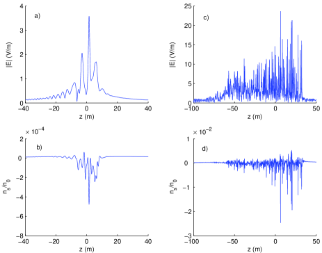
Figure 1: a) Profiles of the amplitude of Langmuir electric field, $|E|$ and b) the electron number density perturbation $n_{s}/n_{0}$ for $E_{\rm pump}=1.0\times 10^{-4}\,\mathrm{V/m}$. c) and d): The same as a) and b) but for $E_{\rm pump}=1.0\times 10^{-3}\,\mathrm{V/m}$. The other parameters are $L=50\,\mathrm{km}$, $\gamma_{L}=1.0\times 10^{3}\,\mathrm{s}^{-1}$, and $\gamma_{s}=1.0\times 10^{3}\,\mathrm{s}^{-1}$.

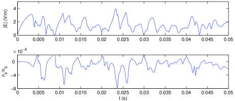
Figure 2: The time-dependent amplitude at $z=0$ of the Langmuir electric field $|E|$ (upper panel) and of the electron number density perturbation $n_{s}/n_{0}$ (lower panel) for $E_{\rm pump}=1.0\times 10^{-4}\,\mathrm{V/m}$. The other parameters are $L=50\,\mathrm{km}$, $\gamma_{L}=1.0\times 10^{3}\,\mathrm{s}^{-1}$, and $\gamma_{s}=1.0\times 10^{3}\,\mathrm{s}^{-1}$.

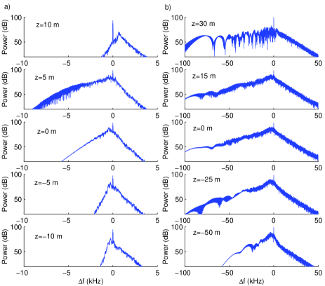
Figure 3: Frequency spectra (in dB) of $E$ at different altitudes, a) $z=10\,\mathrm{m}$, $z=5\,\mathrm{m}$, $z=0\,\mathrm{m}$, $z=-5\,\mathrm{m}$, and $z=-10\,\mathrm{m}$, (top to bottom panel), for $E_{\rm pump}=10^{-4}\,\mathrm{V/m}$ and b) $z=30\,\mathrm{m}$, $z=15\,\mathrm{m}$, $z=0\,\mathrm{m}$, $z=-25\,\mathrm{m}$, and $z=-50\,\mathrm{m}$, (top to bottom panel), for $E_{\rm pump}=10^{-3}\,\mathrm{V/m}$. The other parameters are $L=50\,\mathrm{km}$, $\gamma_{L}=1.0\times 10^{3}\,\mathrm{s}^{-1}$, and $\gamma_{s}=1.0\times 10^{3}\,\mathrm{s}^{-1}$.

In order to investigate the nonlinear dynamics and spectral features of the Zakharov system, we have solved Eqs. (1) and (2) for different sets of parameters. We have used $n_{0}=5\times 10^{11}\,\mathrm{m}^{-3}$, $T_{e}=T_{i}=2000\,\mathrm{K}$, and we have used $m_{i}=26.8\times 10^{-27}\,\mathrm{kg}$ (oxygen ions) in our simulations, so that $\omega_{pe}=4.0\times 10^{7}\,\mathrm{s}^{-1}$, $v_{Te}=1.7\times 10^{5}\,\mathrm{m/s}$ and $C_{s}=2.0\times 10^{3}\,\mathrm{m/s}$. The pump frequency, which is set equal to the local plasma frequency, is $f_{0}=\omega_{pe}/2\pi=6.34\,\mathrm{MHz}$. In the numerical procedure, the Zakharov system was advanced in time with a standard fourth-order Runge-Kutta scheme with a timestep of $10^{-6}\,\mathrm{s}$. The spatial derivatives were approximated with centered, second-order difference approximations with a spatial grid spacing of $5\,\mathrm{cm}$. For weaker pump fields $E_{\rm pump}$ of order $10^{-4}\,\mathrm{V/m}$, we used the spatial domain $-100\,\mathrm{m}\leq z\leq 100\,\mathrm{m}$, and for the stronger pump fields of order $10^{-3}\,\mathrm{V/m}$, we used the spatial domain $-200\,\mathrm{m}\leq z\leq 200\,\mathrm{m}$.

In Fig. 1, we show the profiles of the electric field and the density fluctuations at the end of the simulation, for two different values of the pump field. For a pump field of $E_{\rm pump}=0.1\mathrm{mV/s}$ [panels a) and b)], we see an excited electrostatic field of the order $|E|\sim 3\mathrm{V/m}$ correlated with a density depletion of $n_{s}/n_{0}\sim-4\times 10^{-4}$. The turbulent field is localized in a relatively small interval of $z$ between $-10\,\mathrm{m}$ and $10\,\mathrm{m}$, correlated with electric field maxima are density minima. For the larger pump field $E_{\rm pump}=1.0\,\mathrm{V/m}$, displayed in panels c) and d), the turbulence takes place in a larger altitude interval, between $z\simeq-60\,\mathrm{m}$ and $z\simeq 30\,\mathrm{m}$. Here, the Langmuir field is larger, of the order $10$–$20\,\mathrm{V/m}$, and the maximum density depletion, correlated with electric field maxima, is of the order $n_{s}/n_{0}\sim-10^{-2}$.

The time dependent amplitude of the Langmuir field and the density fluctuations at $z=0$ are shown in Fig. 2, for the first 50 ms (physical time). After an initial growth phase of the fields during the first 3 ms, the fluctuations enter a steady-state turbulent phase during the rest of the time. In Fig. 3, we are analyzing the frequency spectrum of the electric field at different altitudes. In order to obtain the frequency spectrum at each altitude, the simulation was run for $500\,\mathrm{ms}$. The time series of the electric field was subdivided into five time-slices of $100\,\mathrm{ms}$, and each time slice is Fourier transformed in time with a Hamming window. Finally, the average is taken of the five power spectra. The averaged power spectrum (in dB) is visualized in Fig. 3 for $E_{\rm pump}=0.1\,\mathrm{mV/m}$ and $E_{\rm pump}=1\,\mathrm{mV/m}$, at different altitudes. We see that especially the the down-shifted part of the power spectrum differs significantly between different altitudes, while the upshifted part of the spectra vary in their amplitudes but their logarithmic slopes are almost the same at different altitudes. In column a) of Fig. 3, we see that the spectrum is much wider at $z=5$ m than at $z=-5$ m. Hence, in situ measurements by satellites or rockets would be very sensitive to the exact location of the measuring probe. In a thought ground-based experiment, the electrostatic turbulence converts to electromagnetic radiation by some process [Stubbe et al., 1984], and the escaping radiation is monitored by receiving equipment of the ground. The conversion process may involve the mode-conversion of the electrostatic waves against density gradients, resulting in a mixture of frequency components from different altitudes in the resultant electromagnetic radiation. The radiation field from an extended body can be expressed in terms of an integral over the retarded current density. For electrostatic turbulence, the current density and electrostatic field are linked by the Maxwell equation $\partial{\bf E}/\partial t=-{\bf j}/\varepsilon_{0}$, and hence the radiation field is proportional to the spatial integral of the electrostatic field over the turbulent region. We here do not model in detail the conversion process but will assume that the escaping radiation contains frequency components from the spatial average of the electrostatic field (possibly modified by the propagation characteristics of the ionospheric plasma). This model may be valid as long as the wavelengths of the electrostatic waves are much smaller than that of the vacuum electromagnetic waves. In our case the electrostatic waves are on decimeter or meter scale, while the electromagnetic waves are $\sim 60\,\mathrm{m}$. Hence, we have taken the spatial average of the complex electric field $E$ over the simulation box. The spatially averaged electric field is Fourier analyzed in a similar manner as in Fig. 3, and the resulting frequency spectra are plotted in Figs. 4–7 for different sets of parameters.

In principle, the eight physical parameters that can be varied are $E_{\rm pump}$, $L$, $\gamma_{L}$, $\gamma_{s}$, $T_{e}$, $T_{i}$, $n_{0}$, and $m_{i}$. However, the number of parameters can be reduced by normalizing the system, in the spirit of, e.g., Morales and Lee [1977]. Introducing dimensionless, primed variables according to

$$t=({3v_{Te}^{2}}/{2C_{s}^{2}\omega_{pe}})t^{\prime},$$ (3)

$$x=({3v_{Te}^{2}}/{2C_{s}\omega_{pe}})x^{\prime},$$ (4)

$$n_{s}=({4C_{s}^{2}n_{0}}/{3v_{Te}^{2}})n_{s}^{\prime},$$ (5)

$$E=({4C_{s}}/{v_{Te}})({n_{0}m_{i}C_{s}^{2}}/{3\varepsilon_{0}})^{1/2}E^{\prime},$$ (6)

$$E_{\rm pump}=({16C_{s}^{3}}/{3v_{Te}^{3}})({n_{0}m_{i}C_{s}^{2}}/{3\varepsilon_{0}})^{1/2}E_{\rm pump}^{\prime},$$ (7)

$$L=({9v_{Te}^{4}}/{8C_{s}^{3}\omega_{pe}})L^{\prime},$$ (8)

$$\gamma_{L}=({4C_{s}^{2}\omega_{pe}}/{3v_{Te}^{2}})\gamma_{L}^{\prime},$$ (9)

$$\gamma_{s}=({C_{s}^{2}\omega_{pe}}/{3v_{Te}^{2}})\gamma_{s}^{\prime},\\$$ (10)

the Zakharov system (1)–(2) is transformed into

$$i\frac{\partial E^{\prime}}{\partial t^{\prime}}-\left(\frac{x^{\prime}}{L^{\prime}}+n_{s}^{\prime}-i\gamma_{L}^{\prime}\right)E^{\prime}+\frac{\partial^{2}E^{\prime}}{\partial x^{\prime 2}}=E_{\rm pump}^{\prime}$$ (11)

$$\frac{\partial^{2}n_{s}^{\prime}}{\partial t^{\prime 2}}+\gamma_{s}^{\prime}\frac{\partial n_{s}^{\prime}}{\partial t^{\prime}}-\frac{\partial^{2}n_{s}^{\prime}}{\partial x^{\prime 2}}=\frac{\partial^{2}|E^{\prime}|^{2}}{\partial x^{\prime 2}},$$ (12)

and we see that the scaled system have only four free parameters $L^{\prime}$, $\gamma_{L}^{\prime}$, $E_{\rm pump}^{\prime}$, and $\gamma_{s}^{\prime}$. We can state the similarity principle that for any change of parameters (temperatures, densities, etc.) in the dimensional system such that the dimensionless parameters $L^{\prime}$, $\gamma_{L}^{\prime}$, $E_{\rm pump}^{\prime}$, and $\gamma_{s}^{\prime}$ are unchanged, the system is self-similar, i.e., it will have the same solutions as the original system up to linear scalings. We have chosen to vary only the four parameters $E_{\rm pump}$, $L$, $\gamma_{L}$ and $\gamma_{s}$ in our numerical simulations, while keeping the other parameters constant.

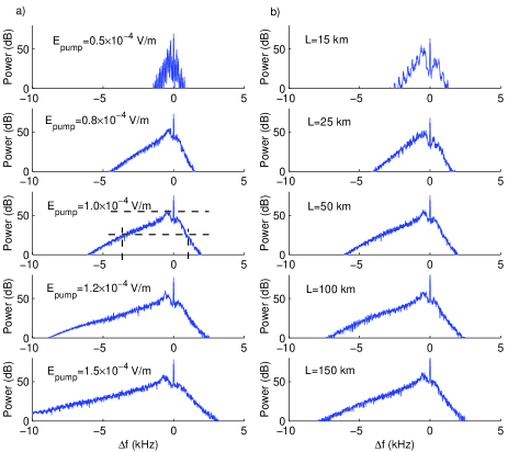
Figure 4: a) Frequency spectra (in dB) of $E$ (spatially averaged) for different pump amplitudes $E_{\rm pump}=0.5\times 10^{-4}\,\mathrm{V/m}$, $E_{\rm pump}=0.8\times 10^{-4}\,\mathrm{V/m}$, $E_{\rm pump}=1.0\times 10^{-4}\,\mathrm{V/m}$, $E_{\rm pump}=1.2\times 10^{-4}\,\mathrm{V/m}$, and $E_{\rm pump}=1.5\times 10^{-4}\,\mathrm{V/m}$ (top to bottom panel), for $L=50\,\mathrm{km}$. The spectral width is defined as the frequency difference between the high-frequency and low-frequency points where the power has dropped 30 dB compared to the downshifted maximum, as indicated with dashed lines for the case $E_{\rm pump}=1.0\times 10^{-4}$ V/m; here the spectral width is approximately 5 kHz. b) Frequency spectra (in dB) of $E$ (spatially averaged) for different ionospheric length scales $L=15\,\mathrm{km}$, $L=25\,\mathrm{km}$, $L=50\,\mathrm{km}$, $L=100\,\mathrm{km}$, and $L=150\,\mathrm{km}$ (top to bottom panel), for $E_{\rm pump}=1.0\times 10^{-4}\,\mathrm{V/m}$. The other parameters are $\gamma_{L}=1.0\times 10^{3}\,\mathrm{s}^{-1}$ and $\gamma_{s}=1.0\times 10^{3}\,\mathrm{s}^{-1}$

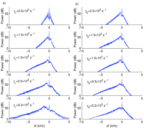
Figure 5: a) Frequency spectra (in dB) of $E$ (spatially averaged) for electron collision frequencies $\gamma_{L}=2.0\times 10^{3}\,\mathrm{s}^{-1}$, $\gamma_{L}=1.5\times 10^{3}\,\mathrm{s}^{-1}$, $\gamma_{L}=1.0\times 10^{3}\,\mathrm{s}^{-1}$, $\gamma_{L}=0.5\times 10^{3}\,\mathrm{s}^{-1}$, and $\gamma_{L}=0.2\times 10^{3}\,\mathrm{s}^{-1}$ (top to bottom panel), for $\gamma_{s}=1.0\times 10^{3}\,\mathrm{s}^{-1}$. b) Frequency spectra (in dB) of $E$ (spatially averaged) for different ion collision frequencies $\gamma_{L}=2.0\times 10^{3}\,\mathrm{s}^{-1}$, $\gamma_{s}=1.5\times 10^{3}\,\mathrm{s}^{-1}$, $\gamma_{s}=1.0\times 10^{3}\,\mathrm{s}^{-1}$, $\gamma_{s}=0.5\times 10^{3}\,\mathrm{s}^{-1}$, and $\gamma_{s}=0.2\times 10^{3}\,\mathrm{s}^{-1}$ (top to bottom panel), for $\gamma_{L}=1.0\times 10^{3}\,\mathrm{s}^{-1}$. The other parameters are $L=50\,\mathrm{km}$ and $E_{\rm pump}=1.0\times 10^{-4}\,\mathrm{V/m}$.

Figure 6: a) Frequency spectra (in dB) of $E$ (spatially averaged) for different pump amplitudes $E_{\rm pump}=0.5\times 10^{-3}\,\mathrm{V/m}$, $E_{\rm pump}=1.0\times 10^{-3}\,\mathrm{V/m}$, and $E_{\rm pump}=2\times 10^{-3}\,\mathrm{V/m}$ (top to bottom panel), for $L=50\,\mathrm{km}$. We have indicated the spectral width with dashed lines, in the same manner as in Fig. 4, for the case $E_{\rm pump}=1.0\times 10^{-3}$ V/m; here the spectral width is approximately $50$ kHz. b) Frequency spectra (in dB) of $E$ (spatially averaged) for different ionospheric length scales $L=25\,\mathrm{km}$, $L=50\,\mathrm{km}$, and $L=100\,\mathrm{km}$ (top to bottom panel), for $E_{\rm pump}=1.0\times 10^{-3}\,\mathrm{V/m}$. The other parameters are $\gamma_{L}=1.0\times 10^{3}\,\mathrm{s}^{-1}$ and $\gamma_{s}=1.0\times 10^{3}\,\mathrm{s}^{-1}$.

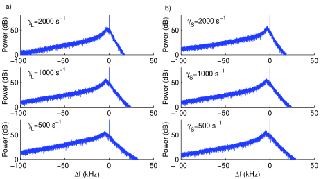
Figure 7: a) Frequency spectra (in dB) of $E$ (spatially averaged) for electron collision frequencies $\gamma_{L}=2.0\times 10^{3}\,\mathrm{s}^{-1}$, $\gamma_{L}=1.0\times 10^{3}\,\mathrm{s}^{-1}$, and $\gamma_{L}=0.5\times 10^{3}\,\mathrm{s}^{-1}$, (top to bottom panel), for $\gamma_{s}=1.0\times 10^{3}\,\mathrm{s}^{-1}$. b) Frequency spectra (in dB) of $E$ (spatially averaged) for different ion collision frequencies $\gamma_{s}=2.0\times 10^{3}\,\mathrm{s}^{-1}$, $\gamma_{s}=1.0\times 10^{3}\,\mathrm{s}^{-1}$, and $\gamma_{s}=0.5\times 10^{3}\,\mathrm{s}^{-1}$, (top to bottom panel), for $\gamma_{L}=1.0\times 10^{3}\,\mathrm{s}^{-1}$. The other parameters are $L=50\,\mathrm{km}$ and $E_{\rm pump}=1.0\times 10^{-3}\,\mathrm{V/m}$.

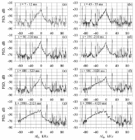
Figure 8: a) SEE spectra recorded at the Sura heating facility in Nizhny Novgorod, Russia, on 25 September 1991 at 13:30–13:50 LT. The spectra are measured at different times (indicated in the boxes) after the switch-on of the pump wave, in a 10 s on, 50 s off mode with pump frequency 5828 MHz and ERP power 30 MW. The spectra are primarily downshifted, and a slow modification of the spectra can be seen, with wider spectra at later times. The narrow spikes are due to interfering radio stations. (After Frolov et al. [2004].)

All the spectra in Figs. 4–7 have some common features. The spectra are asymmetric, where the downshifted part of the frequency spectrum is about three times wider than the upshifted one, although the relative width seems to increase for the downshifted spectrum for larger pump amplitude; see Figs. 6 and 7. We also see a downshifted maximum in the spectra, whose downshift varies from a few kHz up to $\sim 5\,\mathrm{kHz}$, depending on the parameters. These general spectral features are frequently observed in experiments [Thidé et al., 1982, 1989; Thidé, 1990; Frolov et al., 2004]. A few examples of measured SEE spectra are shown in Fig. 8 below, where we see asymmetric spectra with downshifted components. We also observe a slow temporal change of the spectrum, which indicates that the plasma parameters in the ionosphere are slowly modified by the large-amplitude electromagnetic wave.

In Fig. 4, we have varied the pump field $E_{\rm pump}$ and the ionospheric length scale $L$. We define the spectral width as the frequency difference between the high-frequency and low-frequency points where the power has dropped 30 dB compared to the downshifted maximum, as indicated with dashed lines in column a) of Fig. 4 for $E_{\rm pump}=1.0\times 10^{-4}$ V/m; here the spectral width is approximately 5 kHz. We see in column a) of Fig. 4 that the spectral width is almost linearly proportional to the amplitude of $E_{\rm pump}$. The spectra also widens for larger ionospheric length scales, seen in column b) of Fig. 4, and the spectral width is approximately proportional to the square root of the length scale $L$. In Fig. 5, we have varied the collision frequencies $\gamma_{L}$ and $\gamma_{S}$. We here see that the width of the spectrum increases for smaller values of $\gamma_{L}$ and $\gamma_{s}$, and is approximately inversely proportional to the square root of $\gamma_{L}$ and $\gamma_{s}$.

In Figs. 6 and 7, we have repeated the simulations for a one order of magnitude larger pump field than in Figs. 4 and 5. The qualitative results are the same in Figs. 6 and 7. In Fig. 6 we see that the with of the spectrum is approximately linearly proportional to $E_{\rm pump}$. Comparing the case $E_{\rm pump}=10^{-3}$ V/m in column a) of Fig. 6, where the spectral with is 50 kHz with the case $E_{\rm pump}=10^{-4}$ V/m in column a) of Fig. 4, where the spectral width is 5 kHz, we see that the linear dependence of the spectral width on the pump amplitude holds over one decade of pump amplitudes. Similar to the results in Figs. 4 and 5, the spectra in Figs. 6 and 7 widen for increasing $L$ and decreasing $\gamma_{L}$ and $\gamma_{s}$, though the downshifted parts of the spectra are slightly less sensitive to variations in these parameters. Hence, the spectral width obeys the approximate scaling law

$$[\Delta f]_{\rm w}\simeq C\frac{E_{\rm pump}L^{1/2}}{\gamma_{L}^{1/2}\gamma_{S}^{1/2}},$$ (13)

where $C$ is a normalization constant that depends on temperatures, the density, etc., but not on $E_{\rm pump}$, $L$, $\gamma_{L}$ or $\gamma_{s}$. The scaling law can also be expressed in terms of the normalized, primed variables in Eq. (12) as

$$[\Delta f^{\prime}]_{\rm w}\simeq C^{\prime}\frac{E_{\rm pump}^{\prime}L^{\prime 1/2}}{\gamma_{L}^{\prime 1/2}\gamma_{S}^{\prime 1/2}},$$ (14)

where $C^{\prime}$ is a numerical scaling factor that does not depend on any physical parameters in the Zakharov system.

By the scaling of the time (3) in the normalized system (12), we have the the relation

$$[\Delta f]_{\rm w}=\frac{2C_{s}^{2}\omega_{pe}}{3v_{Te}^{2}}[\Delta f^{\prime}]_{\rm w}$$ (15)

between the dimensional and dimensionless spectral widths. Inserting (13) and (14) into (15), and eliminating $E_{\rm pump}$, $L$, $\gamma_{L}$ and $\gamma_{s}$ with the help of (7)–(10), we find, after some algebra, the relation $C=[(\sqrt{6}/18)\omega_{pe}^{3/2}C_{s}^{5/2}e/v_{Te}^{4}(m_{e}m_{i})^{1/2}]C^{\prime}$ between the dimensional and dimensionless scaling factors. Hence, the scaling law (13) can be expressed as

$$[\Delta f]_{\rm w}\simeq A^{\prime}\frac{\omega_{pe}^{3/2}C_{s}^{5/2}eE_{\rm pump}L^{1/2}}{v_{Te}^{4}(m_{i}m_{e})^{1/2}\gamma_{L}^{1/2}\gamma_{s}^{1/2}},$$ (16)

where $A^{\prime}=(\sqrt{6}/18)C^{\prime}$ is a numerical, dimensionless factor, which is determined by the definition of the spectral width. As an example, we take the third row from top of panels in Fig. 4, where we see that the spectral width is $[\Delta f]_{\rm w}\simeq 5\times 10^{3}\,\mathrm{Hz}$, and where the parameters are $E_{\rm pump}=10^{-4}\,\mathrm{V/m}$, $L=50\times 10^{3}\,\mathrm{m}$, $\gamma_{L}=\gamma_{s}=10^{3}\,\mathrm{s}^{-1}$, etc. Inserting the spectral width and the parameters into Eq. (16), we determine the scaling factor to $A^{\prime}=4$. We have thus in Eq. (16) a quantitative measure of the dependence of the frequency spectrum on the physical parameters in the ionosphere.

Returning to the experimental results in Fig. 8, we see that the spectral width of the SEE spectrum increases slowly with time, from approximately 40 kHz in the time intervals during the first second, to approximately 80–90 kHz after 2–4 seconds. This could possibly be due to an increase of the electron temperature, so that $T_{e}\gg T_{i}$, and a resulting decrease of the ion Landau damping $\gamma_{s}$ [Krall and Trivelpiece, 1973] with time, which in turn would lead to an increase of the spectral width according to our scaling law (16).

IV Summary

In conclusion, we have performed a simulation study of Langmuir turbulence with parameters relevant for the F layer in the Earth’s ionosphere. We have used a Zakharov model, including collisions and an ionospheric plasma homogeneity, whose length scale is of the order $10$–$100$ km. The energy source is assumed to be provided by electromagnetic waves [Thidé et al., 1982] in controlled ionospheric wave injection experiments, and is modeled by a constant source term in the Zakharov equation. We have analyzed the frequency spectra for different sets of parameters and different altitudes relative to the classical turning point of the Langmuir waves. By a parametric study, we have derived a simple scaling law, which links the spectral width of the turbulent frequency spectrum to the physical parameters in the ionosphere. The scaling law provides a quantitative relation between the physical parameters (temperatures, electron number density, ionospheric length scale, etc.) and the observed frequency spectrum. An application of our results is to compare our scaling law with SEE spectra, with the assumption that the processes creating the SEE reflect the spectral structure of the turbulent $E$ field via mode conversion of electrostatic waves to electromagnetic radiation.

Acknowledgment This work was supported financially by the Swedish Research Council (VR).

References

- Carozzi et al. [2002] Carozzi, T. D., B. Thidé, S. M. Grach, T. B. Leyser, M. Holz, G. P. Komrakov, V. L. Frolov, and E. N. Sergeev (2002) Stimulated electromagnetic emissions during pump frequency sweep through fourth electron cyclotron harmonic, J. Geophys. Res., 107(A9), 1253, doi:10.1029/2001JA005082.
- Cros et al. [1991] Cros, B., J. Godiot, G. Matthieussent, and A. Héron (1991) Laboratory simulation of ionospheric heating experiment, Geophys. Res. Lett., 18(8), 1623–1626.
- DuBois et al. [1991] Dubois, D. F., H. A. Rose, and D. Russell (1991) Coexistence of parametric decay cascades and caviton collapse at subcritical densities, Phys. Rev. Lett., 66, 1970–1973.
- DuBois et al. [1993] Dubois, D. F., A. Hanssen, H. A. Rose, and D. Russell (1993) Space and time distribution of HF excited Langmuir turbulence in the ionosphere: Comparison of theory and experiment J. Geophys. Res., 98(A10) 17543–17568.
- Forme [1993] Forme, F. R. E. (1993) A new interpretation on the origin of enhanced ion-acoustic fluctuations in the upper atmosphere, Geophys. Res. Lett., 20, 2347 -2350.
- Foster et al. [1988] Foster, J. C., C. del Pozo, K. Groves, and J.-P. St. Maurice (1988) Radar observations of the onset of current driven instabilities in the topside ionosphere, Geophys. Res. Lett., 15, 160 -163.
- Frolov et al. [2004] Frolov, V. L., E. N. Sergeev, G. P. Komrakov, P. Stubbe, B. Thidé, M. Waldenvik, E. Veszelei, T. B. Leyser (2004) Ponderomotive narrow continuum (NCp) component in stimulated electromagnetic emission spectra, J. Geophys. Res., 109, A07304/1–21.
- Guio and Forme [2006] Guio, P., F. Forme (2006) Zakharov simulations of Langmuir turbulence: Effects on the ion-acoustic waves in incoherent scatteroing, Phys. Plasmas, 13, 122902.
- Hansen et al. [1992] Hanssen, A., E. Mjølhus, D. F. Dubois and H. A. Rose (1992) Numerical test of the weak turbulence approximation to ionospheric Langmuir turbulence, J. Geophys. Res., 97(A8) 1992, 12073–12091.
- Kim et al. [1974] Kim, H. C., R. L. Stenzel, and A. Y. Wong (1974) Development of ”cavitons” and trapping of rf field, Phys. Rev. Lett., 33(15), 886–889.
- Krall and Trivelpiece [1973] Krall, N. A., and A. W. Trivelpiece (1973) Principles of Plasma Physics (McGraw-Hill, New York).
-
Leyser [2001]
Leyser, T. B. (2001) Stimulated electromagnetic emissions by
high-frequency electromagnetic pumping of the ionospheric plasma,
Space Sci. Rev., 98, 223 -328.
- Mjølhus [1990] Mjølhus, E. (1990), On linear conversion in a magnetized plasma, Radio Sci. 25(6), 1321–1339.
- Mjølhus [2003] Mjølhus, E., E. Helmersen, and D. F. DuBois (2003) Geometric aspects of HF driven Langmuir turbulence in the ionosphere, Nonlin. Proc. Geophys., 10, 151- 177.
- Morales and Lee [1974] Morales, G. J. and Y. C. Lee (1974) Ponderomotive-force effects in a nonuniform plasma, Phys. Rev. Lett., 33(17), 1016–1019.
- Morales and Lee [1977] Morales, G. and Y. C. Lee (1977) Generation of density cavities and localized electric fields in nonuniform plasma, Phys. Fluids., 20, 1135-1147.
- Nicholson et al. [1984] Nicholson, D. R., G. L. Payne, R. M. Downie, and J. P. Sheerin (1984) Solitons versus parametric instabilities during ionospheric heating, Phys. Rev. Lett., 52, 2152-2155.
- Robinson [1997] Robinson, P. A. (1997) Nonlinear wave collapse and strong turbulence, Rev. Mod. Phys., 69, 507–574.
- Sedgemore-Schulthess and St. Maurice [2001] Sedgemore-Schulthess, F. and J.-P. St. Maurice (2001) Naturally enhanced ion-acoustic spectra and their interpretation, Surv. Geophys., 22, 55 -92, doi:10.1023/A:1010691026863.
- Stubbe et al. [1984] Stubbe, P., H. Kopka, B. Thidé, and H. Derblom (1984) Stimulated electromagnetic emission: A new technique to study the parametric decay instability in the ionosphere, J. Geophys. Res., 89, 7523–7536.
- Thidé et al. [1982] Thidé, B., H. Kopka and P. Stubbe (1982) Phys. Rev. Lett., 49, 1561–1564.
- Thidé et al. [1989] Thidé, B., Å. Hedberg, J. A. Fejer, M. Sulzer (1989) First observation of stimulated electromagnetic emission at Arecibo, Geophys. Res. Lett., 16, 369–372.
- Thidé [1990] Thidé, B. (1990) Stimulated scattering of large amplitude waves in the ionosphere: Experimental results, Phys. Scr., T30, 170–180.
- Wong et al. [1987] Wong, A. Y., T. Tanikawa, and A. Kuthi (1987) Observations of ionospheric cavitons, Phys. Rev. Lett., 58(13), 1375–1378.