The Trade-off between Processing Gains of an Impulse Radio UWB System in the Presence of Timing Jitter${}^{\textrm{\small{1}}}$

Abstract

In time hopping impulse radio, $N_{f}$ pulses of duration $T_{c}$ are transmitted for each information symbol. This gives rise to two types of processing gain: (i) pulse combining gain, which is a factor $N_{f}$, and (ii) pulse spreading gain, which is $N_{c}=T_{f}/T_{c}$, where $T_{f}$ is the mean interval between two subsequent pulses. This paper investigates the trade-off between these two types of processing gain in the presence of timing jitter. First, an additive white Gaussian noise (AWGN) channel is considered and approximate closed form expressions for bit error probability are derived for impulse radio systems with and without pulse-based polarity randomization. Both symbol-synchronous and chip-synchronous scenarios are considered. The effects of multiple-access interference and timing jitter on the selection of optimal system parameters are explained through theoretical analysis. Finally, a multipath scenario is considered and the trade-off between processing gains of a synchronous impulse radio system with pulse-based polarity randomization is analyzed. The effects of the timing jitter, multiple-access interference and inter-frame interference are investigated. Simulation studies support the theoretical results.

Index Terms— Impulse radio ultra-wideband (IR-UWB), timing jitter, multiple-access interference (MAI), inter-frame interference (IFI), Rake receiver.

I Introduction

Recently, communication systems that employ ultra-wideband (UWB) signals have drawn considerable attention. UWB systems occupy a bandwidth larger than 500 MHz, and they can coexist with incumbent systems in the same frequency range due to large spreading factors and low power spectral densities. Recent Federal Communications Commission (FCC) rulings [1], [2] specify the regulations for UWB systems in the US.

Commonly, impulse radio (IR) systems, which transmit very short pulses with a low duty cycle, are employed to implement UWB systems [3]-[5]. Although the short duration of UWB pulses is advantageous for precise positioning applications [6], it also presents practical difficulties such as synchronization, which requires efficient search strategies [7]. In an IR system, a train of pulses is sent and information is usually conveyed by the positions or the amplitudes of the pulses, which correspond to pulse position modulation (PPM) and pulse amplitude modulation (PAM), respectively. Also, in order to prevent catastrophic collisions among different users and thus provide robustness against multiple access interference, each information symbol is represented not by one pulse but by a sequence of pulses and the locations of the pulses within the sequence are determined by a pseudo-random time-hopping (TH) sequence [3].

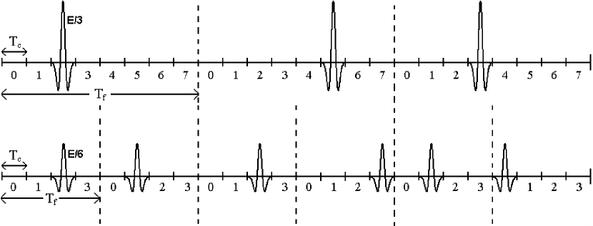
Figure 1: Two different cases for a BPSK-modulated TH-IR system without pulse-based polarity randomization when $N=24$. For the first case, $N_{c}=8$, $N_{f}=3$, and the pulse energy is $E/3$. For the second case, $N_{c}=4$, $N_{f}=6$, and the pulse energy is $E/6$.

The number of pulses that are sent for each information symbol is denoted by $N_{f}$. This first type of processing gain is called the pulse combining gain. The second type of processing gain $N_{c}$ is the pulse spreading gain, and is defined as the ratio of average time between the two consecutive transmissions ($T_{f}$) and the actual transmission time ($T_{c}$); that is, $N_{c}=T_{f}/T_{c}$. The total processing gain is defined as $N=N_{c}N_{f}$ and assumed to be fixed and large [8]. The aim of this paper is to investigate the trade-off between the two types of processing gain, $N_{c}$ and $N_{f}$, and to calculate the optimal $N_{c}$ ($N_{f}$) value such that bit error probability (BEP) of the system is minimized⁵. In other words, the problem is to decide whether or not sending more pulses each with less energy is more desirable in terms of BEP performance than sending fewer pulses each with more energy (Figure 1).

This problem is originally investigated in [8]. Also [9] analyzed the problem from an information theoretic point of view for the single-user case. In [8], it is concluded that in multiuser flat fading channels, the system performance is independent of the pulse combining gain for an IR system with pulse-based polarity randomization and it is in favor of small pulse combining gain for an IR system without pulse-based polarity randomization. However, the analysis is performed in the absence of any timing jitter. Due to the high time resolution of UWB signals, effects of timing jitter are usually not negligible [10]-[12] in IR-UWB systems. As will be observed in this paper, presence of timing jitter has an effect on the trade-off between the processing gains, which can modify the dependency of the BEP expressions on the processing gain parameters. In this paper, the trade-off between the two types of processing gain is investigated in the presence of timing jitter for TH IR systems. First, transmission over an additive white Gaussian noise (AWGN) channel is considered and the trade-off is investigated for IR systems with and without pulse-based polarity randomization. Both symbol-synchronous and chip-synchronous cases are investigated. Also frequency-selective channels are considered and the performance of a downlink IR system with pulse-based polarity randomization is analyzed.

The remainder of the paper is organized as follows. Section II describes the signal model for an IR system. Section III investigates the trade-off between processing gain parameters for IR systems with and without pulse-based polarity randomization over AWGN channels. In each case, the results for symbol-synchronous and chip-synchronous systems are presented. Section IV considers transmission over frequency-selective channels and adopts a quite general Rake receiver structure at the receiver. After the simulation studies in Section V, some conclusions are made in Section VI.

II Signal Model

Consider a BPSK random TH IR system where the transmitted signal from user $k$ in an $N_{u}$-user setting is represented by the following model:

$$s^{(k)}_{{\rm{tx}}}(t)=\sqrt{\frac{E_{k}}{N_{f}}}\sum_{j=-\infty}^{\infty}d^{(k)}_{j}\,b^{(k)}_{\lfloor j/N_{f}\rfloor}w_{{\rm{tx}}}(t-jT_{f}-c^{(k)}_{j}T_{c}-\epsilon_{j}^{(k)}),$$ (1)

where $w_{{\rm{tx}}}(t)$ is the transmitted UWB pulse, $E_{k}$ is the bit energy of user $k$, $\epsilon_{j}^{(k)}$ is the timing jitter at $j$th pulse of the $k$th user, $T_{f}$ is the average time between two consecutive pulses (also called the “frame” time), $T_{c}$ is the pulse interval, $N_{f}$ is the number of pulses representing one information symbol, which is called the pulse combining gain, and $b^{(k)}_{\lfloor j/N_{f}\rfloor}\in\{+1,-1\}$ is the information symbol transmitted by user $k$. In order to allow the channel to be shared by many users and avoid catastrophic collisions, a random TH sequence $\{c^{(k)}_{j}\}$ is assigned to each user, where $c^{(k)}_{j}\in\{0,1,...,N_{c}-1\}$ with equal probability, and $c^{(k)}_{j}$ and $c^{(l)}_{i}$ are independent for $(k,j)\neq(l,i)$. This TH sequence provides an additional time shift of $c^{(k)}_{j}T_{c}$ seconds to the $j$th pulse of the $k$th user. Without loss of generality, $T_{f}=N_{c}T_{c}$ is assumed throughout the paper.

Two different IR systems are considered depending on $d^{(k)}_{j}$. For IR systems with pulse-based polarity randomization [13], $d^{(k)}_{j}$ are binary random variables taking values $\pm 1$ with equal probability and are independent for $(k,j)\neq(l,i)$. Complying with the terminology established in [8], such systems will be called “coded” throughout the paper. The systems with $d^{(k)}_{j}=1$, $\forall k,j$ are called “uncoded”. This second type of system is the original proposal for transmission over UWB channels ([3], [14]) while a version of the first type is proposed in [15].

The timing jitter $\epsilon_{j}^{(k)}$ in (1) mainly represents the inaccuracies of the local pulse generators at the transmitters and is modeled as independent and identically distributed (i.i.d.) among the pulses of a given user [16], [17]. That is, $\epsilon^{(k)}_{j}$ for $j=\ldots,-1,0,1,\ldots$ form an i.i.d. sequence. Also the jitter is assumed to be smaller than the pulse duration $T_{c}$, that is, $\underset{j,k}{\max}|\epsilon_{j}^{(k)}|<T_{c}$, which is usually the case for practical situations.

$N=N_{c}N_{f}$ is defined to be the total processing gain of the system. Assuming a large and constant $N$ value [8], the aim is to obtain the optimal $N_{c}$ ($N_{f}$) value that minimizes the BEP of the system.

III AWGN Channels

The received signal over an AWGN channel in an $N_{u}$-user system can be expressed as

$$r(t)=\sum_{k=1}^{N_{u}}\sqrt{\frac{E_{k}}{N_{f}}}\sum_{j=-\infty}^{\infty}d^{(k)}_{j}\,b^{(k)}_{\lfloor j/N_{f}\rfloor}w_{{\rm{rx}}}(t-jT_{f}-c^{(k)}_{j}T_{c}-\epsilon_{j}^{(k)}-\tau^{(k)})+\sigma_{n}n(t),$$ (2)

where $w_{{\rm{rx}}}(t)$ is the received unit-energy UWB pulse, $\tau^{(k)}$ is the delay of user $k$ and $n(t)$ is white Gaussian noise with zero mean and unit spectral density.

Considering a matched filter (MF) receiver, the template signal at the receiver can be expressed as follows, for the $i$th information symbol:

$$s^{(1)}_{{\rm{temp}}}(t)=\sum_{j=iN_{f}}^{(i+1)N_{f}-1}d_{j}^{(1)}w_{{\rm{rx}}}(t-jT_{f}-c^{(1)}_{j}T_{c}-\tau^{(1)}),$$ (3)

where, without loss of generality, user $1$ is assumed to be the user of interest. Also note that no timing jitter is considered for the template signal since the jitter model in the received signal can be considered to account for that jitter as well, without loss of generality.

From (2) and (3), the MF output for user $1$ can be expressed as follows^6,7 :

$$y=\int r(t)s_{{\rm{temp}}}^{(1)}(t)dt\approx\sqrt{\frac{E_{1}}{N_{f}}}\,b_{i}^{(1)}\sum_{j=iN_{f}}^{(i+1)N_{f}-1}\phi_{w}(\epsilon_{j}^{(1)})+a+n,$$ (4)

where the first term is the desired signal part of the output with $\phi_{w}(x)=\int_{-\infty}^{\infty}w_{{\rm{rx}}}(t)w_{{\rm{rx}}}(t-x)dt$ being the autocorrelation function of the UWB pulse, $a$ is the multiple-access interference (MAI) due to other users and $n$ is the output noise, which is approximately distributed as $n\sim\mathcal{N}(0,\,N_{f}\sigma_{n}^{2})$.

The MAI term can be expressed as the sum of interference terms from each user, that is, $a=\sum_{k=2}^{N_{u}}\sqrt{\frac{E_{k}}{N_{f}}}a^{(k)}$, where each interference term is in turn the summation of interference to one pulse of the template signal:

$$a^{(k)}=\sum_{m=iN_{f}}^{(i+1)N_{f}-1}a_{m}^{(k)},$$ (5)

where

$$a_{m}^{(k)}=d_{m}^{(1)}\int w_{{\rm{rx}}}(t-mT_{f}-c_{m}^{(1)}T_{c}-\tau^{(1)})\sum_{j=-\infty}^{\infty}d_{j}^{(k)}b^{(k)}_{\lfloor j/N_{f}\rfloor}w_{{\rm{rx}}}(t-jT_{f}-c^{(k)}_{j}T_{c}-\epsilon_{j}^{(k)}-\tau^{(k)})\,dt.$$ (6)

As can be seen from (6), $a_{m}^{(k)}$ denotes the interference from user $k$ to the $m$th pulse of the template signal.

In this study, we consider chip-synchronous and symbol-synchronous situations for the simplicity of the expressions. However, the current study can be extended to asynchronous systems as well [18]. In this paper, we will see that for coded systems, the effect of the MAI is the same whether the users are symbol-synchronous or chip-synchronous. However, for uncoded systems, the average power of the MAI is larger, hence the BEP is higher, when the users are symbol-synchronous.

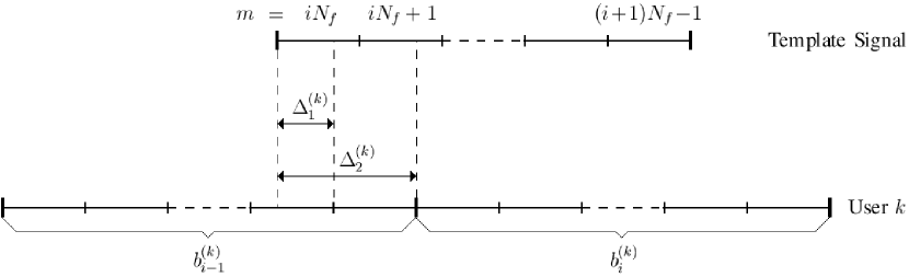
Figure 2: The positions of the template signal and the signal of user $k$.

We assume, without loss of generality, that the delay of the first user, $\tau^{(1)}$, is zero. Then, $\tau^{(k)}=0$ $\forall k$ for symbol-synchronous systems. For chip-synchronous systems, $\tau^{(k)}=\Delta_{2}^{(k)}T_{c}$, where $\Delta_{2}^{(k)}\in\{0,1,\ldots,N-1\}$ with equal probability. Also let $\Delta^{(k)}_{1}$ be the offset between the frames of user $1$ and $k$. Then, $\Delta^{(k)}_{1}=\mod\{\Delta_{2}^{(k)},N_{c}\}$ and obviously, $\Delta_{1}^{(k)}\in\{0,1,...,N_{c}-1\}$ with equal probability (Figure 2).

III-A Coded Systems

For symbol-synchronous and chip-synchronous coded systems, the following lemma approximates the probability distribution of $a^{(k)}$ in (5):

Lemma III.1

As $N\longrightarrow\infty$ and $\frac{N_{f}}{N_{c}}\longrightarrow c>0$, $a^{(k)}$ is asymptotically normally distributed as

$$a^{(k)}\sim{\mathcal{N}}(0\,,\,\gamma^{(k)}_{2}N_{f}/N_{c}),$$ (7)

where $\gamma^{(k)}_{2}=\textrm{E}\{\phi_{w}^{2}(\epsilon^{(k)})\}+\textrm{E}\{\phi_{w}^{2}(T_{c}-|\epsilon^{(k)}|)\}$.

Proof: See Appendix A-A.

From the previous lemma, it is observed that the distribution of the MAI is the same whether there is symbol-synchronization or chip-synchronization among the users, which is due to the use of random polarity codes in each frame.

From (4) and (7), the BEP of the coded IR system conditioned on the timing jitter of user $1$ can be approximated as follows:

$$P_{e|\boldsymbol{\epsilon}_{i}^{(1)}}\approx Q\left(\frac{\sqrt{\frac{E_{1}}{N_{f}}}\sum_{j=iN_{f}}^{(i+1)N_{f}-1}\phi_{w}(\epsilon_{j}^{(1)})}{\sqrt{\frac{1}{N_{c}}\sum_{k=2}^{N_{u}}E_{k}\gamma^{(k)}_{2}+N_{f}\sigma_{n}^{2}}}\right),$$ (8)

where $\boldsymbol{\epsilon}_{i}^{(1)}=[\epsilon^{(1)}_{iN_{f}}\ldots\epsilon^{(1)}_{(i+1)N_{f}-1}]$.

For large values of $N_{f}$, it follows from the Central Limit Theorem (CLT) that $\frac{1}{\sqrt{N_{f}}}\sum_{j=iN_{f}}^{(i+1)N_{f}-1}[\phi_{w}(\epsilon_{j}^{(1)})-\textrm{E}\{\phi_{w}(\epsilon_{j}^{(1)})\}]$ is approximately Gaussian. Then, using the relation $\textrm{E}\{Q(X)\}=Q\left(\frac{\hat{\mu}}{\sqrt{1+\hat{\sigma}^{2}}}\right)$ for $X\sim\mathcal{N}(\hat{\mu},\hat{\sigma}^{2})$ [19], the unconditional BEP can be expressed approximately as follows:

$$P_{e}\approx Q\left(\frac{\sqrt{E_{1}}\mu}{\sqrt{\frac{E_{1}\sigma^{2}}{N_{f}}+\frac{1}{N}\sum_{k=2}^{N_{u}}E_{k}\gamma^{(k)}_{2}+\sigma_{n}^{2}}}\right),$$ (9)

where $\mu=\textrm{E}\{\phi_{w}(\epsilon_{j}^{(1)})\}$ and $\sigma^{2}=\textrm{Var}\{\phi_{w}(\epsilon_{j}^{(1)})\}$.

From (9), it is observed that the BEP decreases as $N_{f}$ increases, if the first term in the denominator is significant. In other words, the BEP gets smaller for larger number of pulses per information symbol. We observe from (9) that the second term in the denominator, which is due to the MAI, depends on $N_{c}$ and $N_{f}$ only through their product $N=N_{c}N_{f}$. Therefore, the MAI has no effect on the trade-off between processing gains for a fixed total processing gain $N$. The only term that depends on how to distribute $N$ between $N_{c}$ and $N_{f}$ is the first term in the denominator, which reflects the effect of timing jitter. This effect is mitigated by choosing small $N_{c}$, or large $N_{f}$, which means sending more pulses per information bit. Therefore, for a coded system, keeping $N_{f}$ large can help reduce the BEP. Also note that in the absence of timing jitter, (9) reduces to $P_{e}\approx Q\left(\frac{\sqrt{E_{1}}}{\sqrt{\frac{1}{N}\sum_{k=2}^{N_{u}}E_{k}+\sigma_{n}^{2}}}\right)$, in which case there is no effect of processing gain parameters on BEP performance, as stated in [8].

III-B Uncoded Systems

For coded systems, we have observed that the system performance is the same for symbol-synchronous and chip-synchronous scenarios. For an uncoded system, the effect of MAI changes depending on the type of synchronism, as we study in this section.

First consider a symbol-synchronous system; that is, $\tau^{(k)}=0$ $\forall k$ in (2). In this case, following lemma approximates the probability distribution of $a^{(k)}$ in (5) for an uncoded system:

Lemma III.2

As $N\longrightarrow\infty$ and $\frac{N_{f}}{N_{c}}\longrightarrow c>0$, $a^{(k)}$ conditioned on the information bit $b_{i}^{(k)}$, is approximately distributed as

$$a^{(k)}|b_{i}^{(k)}\sim{\mathcal{N}}\left(\frac{N_{f}}{N_{c}}b_{i}^{(k)}\gamma^{(k)}_{1}\,,\,\frac{N_{f}}{N_{c}}\left[\gamma^{(k)}_{2}-\frac{(\gamma^{(k)}_{1})^{2}}{N_{c}}+\frac{\beta^{(k)}_{1}}{N_{c}^{2}}+\frac{\beta^{(k)}_{2}}{N_{c}^{3}}\right]\right),$$ (10)

where

$$\gamma^{(k)}_{1} =\textrm{E}\{\phi_{w}(\epsilon^{(k)})\}+\textrm{E}\{\phi_{w}(T_{c}-|\epsilon^{(k)}|)\},\quad\gamma^{(k)}_{2}=\textrm{E}\{\phi_{w}^{2}(\epsilon^{(k)})\}+\textrm{E}\{\phi_{w}^{2}(T_{c}-|\epsilon^{(k)}|)\},$$

$$\beta^{(k)}_{1} =2\textrm{E}\{\phi_{w}(T_{c}-|\epsilon^{(k)}|)\phi_{w}(\epsilon^{(k)})\}-2(\textrm{E}\{\phi_{w}(T_{c}-|\epsilon^{(k)}|)\})^{2}$$

$$+4\int_{-\infty}^{0}\phi_{w}(T_{c}+\epsilon^{(k)})p(\epsilon^{(k)})d\epsilon^{(k)}\int_{0}^{\infty}\phi_{w}(T_{c}-\epsilon^{(k)})p(\epsilon^{(k)})d\epsilon^{(k)},$$

$$\beta^{(k)}_{2} =2(\textrm{E}\{\phi_{w}(T_{c}-|\epsilon^{(k)}|)\})^{2}.$$ (11)

Proof: See Appendix A-B.

Note that for systems with large $N_{c}$, the distribution of $a^{(k)}$ given the information symbol $b_{i}^{(k)}$ can be approximately expressed as $a^{(k)}|b_{i}^{(k)}\sim{\mathcal{N}}\left(b_{i}^{(k)}\gamma^{(k)}_{1}N_{f}/N_{c}\,,\,\frac{N_{f}}{N_{c}}[\gamma^{(k)}_{2}-(\gamma_{1}^{(k)})^{2}/N_{c}]\right)$.

First consider a two-user system. For equiprobable information symbols $\pm 1$, the BEP conditioned on timing jitter of the first user can be shown to be

$$\textrm{P}_{e|\boldsymbol{\epsilon}^{(1)}}\approx\frac{1}{2}\,Q\left(\frac{\frac{\sqrt{E_{1}}}{N_{f}}\sum_{j=iN_{f}}^{(i+1)N_{f}-1}\phi_{w}(\epsilon_{j}^{(1)})+\frac{\sqrt{E_{2}}}{N_{c}}\gamma^{(2)}_{1}}{\sqrt{\frac{E_{2}}{N}[\gamma^{(2)}_{2}-(\gamma^{(2)}_{1})^{2}/N_{c}]+\sigma_{n}^{2}}}\right)+\,\frac{1}{2}\,Q\left(\frac{\frac{\sqrt{E_{1}}}{N_{f}}\sum_{j=iN_{f}}^{(i+1)N_{f}-1}\phi_{w}(\epsilon_{j}^{(1)})-\frac{\sqrt{E_{2}}}{N_{c}}\gamma^{(2)}_{1}}{\sqrt{\frac{E_{2}}{N}[\gamma^{(2)}_{2}-(\gamma^{(2)}_{1})^{2}/N_{c}]+\sigma_{n}^{2}}}\right).$$ (12)

Then, for large $N_{f}$ values, we can again invoke the CLT for $\frac{1}{\sqrt{N_{f}}}\sum_{j=iN_{f}}^{(i+1)N_{f}-1}[\phi_{w}(\epsilon_{j}^{(1)})-\mu]$ and approximate the unconditional BEP as

$$P_{e}\approx\frac{1}{2}Q\left(\frac{\sqrt{E_{1}}\mu+\frac{\sqrt{E_{2}}}{N_{c}}\gamma_{1}^{(2)}}{\sqrt{\frac{E_{1}\sigma^{2}}{N}N_{c}+\frac{E_{2}}{N}[\gamma^{(2)}_{2}-(\gamma^{(2)}_{1})^{2}/N_{c}]+\sigma_{n}^{2}}}\right)+\,\frac{1}{2}Q\left(\frac{\sqrt{E_{1}}\mu-\frac{\sqrt{E_{2}}}{N_{c}}\gamma_{1}^{(2)}}{\sqrt{\frac{E_{1}\sigma^{2}}{N}N_{c}+\frac{E_{2}}{N}[\gamma^{(2)}_{2}-(\gamma^{(2)}_{1})^{2}/N_{c}]+\sigma_{n}^{2}}}\right).$$ (13)

For the multiuser case, assume that all the interfering users have the same energy $E$ and probability distributions of the jitters are i.i.d. for all of them. Then, the total MAI can be approximated by a zero mean Gaussian random variable for sufficiently large number of users, $N_{u}$, and, after similar manipulations, the BEP can be expressed approximately as

$$P_{e}\approx Q\left(\frac{\sqrt{E_{1}}\mu}{\sqrt{\frac{E_{1}\sigma^{2}}{N}N_{c}+(N_{u}-1)E\left(\frac{\gamma_{2}}{N}+\frac{\gamma_{1}^{2}}{N_{c}^{2}}-\frac{\gamma_{1}^{2}}{NN_{c}}\right)+\sigma_{n}^{2}}}\right),$$ (14)

where the user index $k$ is dropped from $\gamma_{1}^{(k)}$ and $\gamma_{2}^{(k)}$ since they are i.i.d. among interfering users.

Considering (14), it is seen that for relatively small $N_{c}$ values, the second term in the denominator, which is the term due to MAI, can become large and cause an increase in the BEP. Similarly, when $N_{c}$ is large, the first term in the denominator can become significant and the BEP can become high again. Therefore, we expect to have an optimal $N_{c}$ value for the interference-limited case. Intuitively, for small $N_{c}$ values, the number of pulses per bit, $N_{f}$, is large. Therefore, we have high BEP due to large amount of MAI. As $N_{c}$ becomes large, the MAI becomes more negligible. However, making $N_{c}$ very large can again cause an increase in BEP since $N_{f}$ becomes small, in which case the effect of timing jitter becomes more significant. The optimal $N_{c}$ ($N_{f}$) value can be approximated by using (14).

Now consider the chip-synchronous case. In this case, the following lemma approximates the distribution of the overall MAI for large number of equal energy interferers:

Lemma III.3

Let $N\longrightarrow\infty$ and $\frac{N_{c}}{N_{f}}\longrightarrow c>0$. Assume that all $(N_{u}-1)$ interfering users have the same bit energy $E$ and i.i.d. jitter statistics. Then, the overall MAI, $a$ in (4), is approximately distributed, for large $N_{u}$, as

$$a\sim{\mathcal{N}}\left(0\,,\,\frac{E(N_{u}-1)}{N_{c}}\left[\gamma_{2}+\frac{(N_{f}-1)[2N_{c}^{2}(N_{f}-1)+1]}{3NN_{c}^{2}}\gamma_{1}^{2}\right]\right),$$ (15)

where $\gamma_{1}$ and $\gamma_{2}$ are as in (III.2).

Proof: The proof is omitted due to space limitations. It mainly depends on some central limit arguments.

Comparing the variance in Lemma III.3 with the variance of the MAI term in the uncoded symbol-synchronous case for large number of equal energy interferers with the same jitter statistics, it can be shown that $\sigma^{2}_{MAI,\,chip}\leq\sigma^{2}_{MAI,\,symb}$ where

$$\sigma^{2}_{MAI,\,symb} =\frac{E(N_{u}-1)}{N_{c}}\left[\gamma_{2}+\frac{N_{f}-1}{N_{c}}\,\gamma_{1}^{2}\right],$$ (16)

$$\sigma^{2}_{MAI,\,chip} =\frac{E(N_{u}-1)}{N_{c}}\left[\gamma_{2}+\frac{(N_{f}-1)[2N_{c}^{2}(N_{f}-1)+1]}{3NN_{c}^{2}}\,\gamma_{1}^{2}\right],$$ (17)

where the equality is satisfied only for $N_{f}=1$.

The reason behind this inequality can be explained as follows: In the uncoded symbol-synchronous case, interference components from a given user to the pulses of the template signal has the same polarity and therefore they add coherently for each user. However, in the chip-synchronous case, interference to some pulses of the template is due to one information bit whereas the interference to the remaining pulses is due to another information bit because there is a misalignment between symbol transmission instants (Figure 2). Since information bits can be $\pm 1$ with equal probability, the interference from a given user to individual pulses of the template signal does not always add coherently. Therefore, the average power of the MAI is smaller in the chip-synchronous case. As the limiting case, consider the coded case, where each individual pulse has a random polarity code. In this case, the overall interference from a user, given the information bit of that user, is zero mean due to the polarity codes. Hence, the overall interference from all users has a smaller average power, given by $\gamma_{2}E(N_{u}-1)/N_{c}$, for equal energy interferers with i.i.d jitter statistics.

By Lemma III.3 and the approximation to the distribution of the signal part of the MF output given the information bit in (4) by a Gaussian random variable, we get

$$P_{e}\approx Q\left(\frac{\sqrt{E_{1}}\mu}{\sqrt{\frac{E_{1}\sigma^{2}}{N}N_{c}+(N_{u}-1)E\left[\frac{\gamma_{2}}{N}+\frac{(N-N_{c})[2N_{c}(N-N_{c})+1]}{3N^{2}N_{c}^{3}}\gamma_{1}^{2}\right]+\sigma_{n}^{2}}}\right),$$ (18)

where $\mu=\textrm{E}\{\phi_{w}(\epsilon_{j}^{(1)})\}$ and $\sigma^{2}=\textrm{Var}\{\phi_{w}(\epsilon_{j}^{(1)})\}$.

Considering (18), we have similar observations as in the symbol-synchronous case. Considering the interference-limited case, for small $N_{c}$ values, the second term in the denominator, which is the term due to the MAI, becomes dominant and causes a large BEP. When $N_{c}$ is large, the MAI becomes less significant since probability of overlaps between pulses decreases. However, for very small $N_{c}$ values, the effect of the timing jitter can become more significant as can be seen from the first term in the denominator and the BEP can increase again. Therefore, in this case, we again expect to see a trade-off between processing gain parameters.

IV Multipath Case

In this section, the effects of the processing gain parameters, $N_{c}$ and $N_{f}$, on the BEP performance of a coded system are investigated in a frequency-selective environment. The following channel model is considered [20], [21]:

$$h(t)=\sum_{l=0}^{L-1}\alpha_{l}\delta(t-\tau_{l}),$$ (19)

where $\alpha_{l}$ and $\tau_{l}$ are, respectively, the fading coefficient and the delay of the $(l+1)$th path. Note that we assume a single cluster without loss of generality of the analysis. In fact, even a multipath channel model with pulse distortions can be incorporated into the analysis as will be explained at the end of the section.

We consider a downlink scenario, where the transmitted symbols are synchronized, and assume $\tau_{0}=0$ without loss of generality. Moreover, for the simplicity of the analysis, the delay of the last path, $\tau_{L-1}$, is set to an integer multiple of the chip interval $T_{c}$; that is, $\tau_{L-1}=(M-1)T_{c}$ where $M$ is an integer. Note that this does not cause a loss in generality since we can always think of a hypothetical path at $T_{c}\lceil\tau_{L-1}/T_{c}\rceil$ with a fading coefficient of zero, with $\lceil x\rceil$ denoting the smallest integer larger than or equal to $x$.

From (1) and (19), the received signal can be expressed as follows:

$$r(t)=\sum_{k=1}^{N_{u}}\sqrt{\frac{E_{k}}{N_{f}}}\sum_{j=-\infty}^{\infty}d_{j}^{(k)}b^{(k)}_{\lfloor j/N_{f}\rfloor}u(t-jT_{f}-c_{j}^{(k)}T_{c}-\epsilon_{j}^{(k)})+\sigma_{n}n(t),$$ (20)

where $n(t)$ is zero mean white Gaussian noise with unit spectral density and $u(t)=\sum_{l=0}^{L-1}\alpha_{l}w_{{\rm{rx}}}(t-\tau_{l})$, with $w_{{\rm{rx}}}(t)$ denoting the received unit energy UWB pulse. $\epsilon_{j}^{(k)}$ is the timing jitter at the transmitted pulse in the $j$th frame of user $k$. We assume that $\epsilon^{(k)}_{j}$ for $j=\ldots,-1,0,1,\ldots$ form an i.i.d. sequence for each user and that $\underset{j,k}{\max}\,|\epsilon_{j}^{(k)}|<T_{c}$.

Consider a generic Rake receiver that combines a number of multipath components of the incoming signal. Rake receivers are considered for UWB systems in order to collect sufficient signal energy from incoming multipath components [22]-[27]. For the $i$th information symbol, the following signal represents the template signal for such a receiver:

$$s_{{\rm{temp}}}^{(1)}(t)=\sum_{j=iN_{f}}^{(i+1)N_{f}-1}d_{j}^{(1)}v_{j}(t-jT_{f}-c_{j}^{(1)}T_{c}),$$ (21)

where user $1$ is considered as the user of interest without loss of generality, $v_{j}(t)=\sum_{l=0}^{L-1}\beta_{l}w_{{\rm{rx}}}(t-\tau_{l}-\hat{\epsilon}_{j,l})$, with $\boldsymbol{\beta}=[\beta_{0}\cdots\beta_{L-1}]$ denoting the Rake combining coefficients and $\hat{\epsilon}_{j,l}$ being the timing jitter at the $l$th finger in the $j$th frame of the template signal. We assume that $\underset{j,l}{\max}\,|\hat{\epsilon}_{j,l}|<T_{c}$ and $\underset{i,j,k,l}{\max}\,|\hat{\epsilon}_{j,l}-\epsilon_{i}^{(k)}|<T_{c}$, which, practically true most of the time, makes sure that a pulse can only interfere with the neighboring chip positions due to timing jitter.

Corresponding to different situations, we consider three different statistics for the jitter at the template signal:

Case-1: The jitter is assumed to be i.i.d. for all different finger and frame indices; that is, $\hat{\epsilon}_{j,l}$ for $(j,l)\in\mathcal{Z}\times\mathcal{L}$ form an i.i.d. sequence, where where $\mathcal{Z}$ is the set of integers and $\mathcal{L}=\{0,1,\ldots,L-1\}$.

Case-2: The same jitter value is assumed for all fingers, and i.i.d. jitters are assumed among different frames. In other words, $\hat{\epsilon}_{j,l_{1}}=\hat{\epsilon}_{j,l_{2}}$ $\forall l_{1},l_{2}$ and $\hat{\epsilon}_{j,l}$ for $j\in\mathcal{Z}$ form an i.i.d. sequence.

Case-3: The same jitter value is assumed in all frames for a given finger, and i.i.d. jitters are assumed among the fingers. In other words, $\hat{\epsilon}_{j_{1},l}=\hat{\epsilon}_{j_{2},l}$ $\forall j_{1},j_{2}$ and $\hat{\epsilon}_{j,l}$ for $l\in{\mathcal{L}}$ form an i.i.d. sequence.

We will consider only Case-1 and Case-2 in the following analysis and an extension of the results to Case-3 will be briefly discussed at the end of the section.

Using (20) and (21), the correlation output for the $i$th symbol can be expressed as

$$y=\int r(t)\,s_{{\rm{temp}}}^{(1)}(t)\,dt=b_{i}^{(1)}\sqrt{\frac{E_{1}}{N_{f}}}\sum_{m=iN_{f}}^{(i+1)N_{f}-1}\phi_{uv}^{(m)}(\epsilon_{m}^{(1)})+\hat{a}+a+n,$$ (22)

where the first term is the desired signal component with $\phi_{uv}^{(m)}(\Delta)=\int u(t-\Delta)v_{m}(t)dt$, $a$ is the MAI, $\hat{a}$ is the inter-frame interference (IFI) and $n=\sigma_{n}\sum_{j=iN_{f}}^{(i+1)N_{f}-1}d_{j}^{(1)}\int v_{j}(t-jT_{f}-c_{j}^{(1)}T_{c})n(t)dt$ is the output noise, which can be shown to be distributed, approximately, as $n\sim\mathcal{N}\left(0\,,\,\sigma_{n}^{2}N_{{\rm{f}}}\bar{E}_{v}\right)$, with $\bar{E}_{v}=\frac{1}{N_{f}}\sum_{j=iN_{f}}^{(i+1)N_{f}-1}\int_{-\infty}^{\infty}v_{j}^{2}(t)dt$, for large $N_{{\rm{f}}}$⁸.

The IFI is the self interference among the pulses of the user of interest, user $1$, which occurs when a pulse in a frame spills over to adjacent frame(s) due to multipath and/or timing jitter and interferes with a pulse in that frame. The overall IFI can be considered as the sum of interference to each frame; that is, $\hat{a}={\sqrt{\frac{E_{1}}{N_{f}}}}\sum_{m=iN_{f}}^{(i+1)N_{f}-1}\hat{a}_{m}$, where the interference to the $m$th pulse can be expressed as

$$\hat{a}_{m}=d_{m}^{(1)}\int v_{m}(t-mT_{f}-c_{m}^{(1)}T_{c})\underset{j\neq m}{\sum_{j=-\infty}^{\infty}}d^{(1)}_{j}\,b^{(1)}_{\lfloor j/N_{f}\rfloor}u(t-jT_{f}-c^{(1)}_{j}T_{c}-\epsilon_{j}^{(1)})dt.$$ (23)

Assume that the delay spread of the channel is not larger than the frame time. In other words, $M\leq N_{c}$. In this case, (23) can be expressed as

$$\hat{a}_{m}=d_{m}^{(1)}\sum_{i\in\{-1,1\}}d_{m+i}^{(1)}b^{(1)}_{\lfloor(m+i)/N_{f}\rfloor}\phi_{uv}^{(m)}\left(iT_{f}+(c_{m+i}^{(1)}-c_{m}^{(1)})T_{c}+\epsilon_{m+i}^{(1)}\right).$$ (24)

Then, using the central limit argument in [28] for dependent sequences, we can obtain the distribution of $\hat{a}$ as follows:

Lemma IV.1

As $N\longrightarrow\infty$ and $\frac{N_{f}}{N_{c}}\longrightarrow c>0$, the IFI $\hat{a}$ is asymptotically normally distributed as

$$\hat{a}\sim{\mathcal{N}}\left(0\,,\,\frac{E_{1}}{N_{c}^{2}}\sum_{j=1}^{M}j\,\textrm{E}\{[\phi_{uv}^{(m)}(jT_{c}+\epsilon_{m+1}^{(1)})+\phi_{uv}^{(m)}(-jT_{c}+\epsilon_{m-1}^{(1)})]^{2}\}\right).$$ (25)

Proof: See Appendix A-C.

Note that the result is true for both Case-1 and Case-2. The only difference between the two cases is the set of jitter variables over which the expectation is taken.

The MAI term in (22) can be expressed as the sum of interference from each user, $a=\sum_{k=2}^{N_{u}}\sqrt{\frac{E_{k}}{N_{f}}}\,a^{(k)}$, where each $a^{(k)}$ can be considered as the sum of interference to each frame of the template signal from the signal of user $k$. That is, $a^{(k)}=\sum_{m=iN_{f}}^{(i+1)N_{f}-1}a_{m}^{(k)}$, where

$$a_{m}^{(k)}=d_{m}^{(1)}\int v_{m}(t-mT_{f}-c_{m}^{(1)}T_{c})\sum_{j=-\infty}^{\infty}d_{j}^{(k)}b^{(k)}_{\lfloor j/N_{f}\rfloor}u(t-jT_{f}-c^{(k)}_{j}T_{c}-\epsilon_{j}^{(k)})\,dt.$$ (26)

Assuming $M\leq N_{c}$, $a_{m}^{(k)}$ can be expressed as

$$a_{m}^{(k)}=d_{m}^{(1)}\sum_{j=m-1}^{m+1}d_{j}^{(k)}b^{(k)}_{\lfloor j/N_{f}\rfloor}\phi_{uv}^{(m)}\left((j-m)T_{f}+(c_{j}^{(k)}-c_{m}^{(1)})T_{c}+\epsilon_{j}^{(k)}\right).$$ (27)

Then, using the same central limit argument [28] as in Lemma IV.1, we obtain the following result:

Lemma IV.2

As $N\longrightarrow\infty$ and $\frac{N_{f}}{N_{c}}\longrightarrow c>0$, the MAI from user $k$, $a^{(k)}$, is asymptotically normally distributed as

$$a^{(k)}\sim{\mathcal{N}}\left(0\,,\,\frac{N_{f}}{N_{c}}\sum_{j=-M}^{M}\textrm{E}\{[\phi_{uv}^{(m)}(jT_{c}+\epsilon^{(k)})]^{2}\}\right).$$ (28)

Proof: See Appendix A-D.

Since we assume that the timing jitter variables at the transmitted pulses in different frames form an i.i.d. sequence for a given user, and the jitter at the template is i.i.d. among different frames, the first term in (22) given the information bit of user $1$ converges to a Gaussian random variable for large $N_{f}$ values. Using this observation and the results of the previous two lemmas, we can express the BEP of the system as

$$P_{e}\approx Q\left(\frac{\sqrt{E_{1}}\,\textrm{E}\{\phi_{uv}^{(m)}(\epsilon^{(1)})\}}{\sqrt{\frac{E_{1}N_{c}}{N}\textrm{Var}\{\phi_{uv}^{(m)}(\epsilon^{(1)})\}+\frac{E_{1}}{N_{c}N}\sigma_{IFI}^{2}+\frac{1}{N}\sum_{k=2}^{N_{u}}E_{k}\sigma_{MAI,k}^{2}+\bar{E}_{v}\sigma_{n}^{2}}}\right),$$ (29)

where

$$\sigma_{IFI}^{2}=\sum_{j=1}^{M}j\,\textrm{E}\{[\phi_{uv}^{(m)}(jT_{c}+\epsilon_{m+1}^{(1)})+\phi_{uv}^{(m)}(-jT_{c}+\epsilon_{m-1}^{(1)})]^{2}\}$$ (30)

and

$$\sigma_{MAI,k}^{2}=\sum_{j=-M}^{M}\textrm{E}\{[\phi_{uv}^{(m)}(jT_{c}+\epsilon^{(k)})]^{2}\}$$ (31)

are independent of the processing gain parameters.

From (29), a trade-off between the effect of the timing jitter and that of the IFI is observed. The first term in the denominator, which is due to the effect of the timing jitter on the desired signal part of the output in (22), can cause an increase in the BEP as $N_{c}$ increases. The second term in the denominator is due to the IFI, which can cause a decrease in the BEP as $N_{c}$ increases; because, as $N_{c}$ increases, the probability of a spill-over from one frame to the next decreases. Hence, large $N_{c}$ values mitigate the effects of IFI. The term due to the MAI (the third term in the denominator) does not depend on $N_{c}$ ($N_{f}$) for a given value of total processing gain $N$. Therefore, it has no effect on the trade-off between processing gains. The optimal value of $N_{c}$ ($N_{f}$) minimizes the BEP by optimally mitigating the opposing effects of the timing jitter and the IFI.

Remark-1: The same conclusions hold for Case-3, in which the timing jitter at the template signal is the same for all frames for a given finger, and i.i.d. among different fingers. In this case, conditioning on the jitter values at different fingers ($\hat{\epsilon}_{j,0}\cdots\hat{\epsilon}_{j,L-1}$), the conditional BEP ($P_{{\rm{e}}}|\hat{\epsilon}_{j,0}\cdots\hat{\epsilon}_{j,L-1}$) can be shown to be as in (29); hence, the same dependence structure on the processing gain parameters is observed. The only difference in this case is that the statistical averages are calculated only over the jitter values at the transmitter.

Remark-2: For the case in which pulses are also distorted by the channel; i.e., pulse shapes in different multipath components are different, the analysis is still valid. Since the results (29)-(31) are in terms of the cross-correlation $\phi_{uv}^{(j)}(\cdot)$ of $u(t)=\sum_{l=0}^{L-1}\alpha_{l}w_{{\rm{rx}}}(t-\tau_{l})$ and $v_{j}(t)=\sum_{l=0}^{L-1}\beta_{l}w_{{\rm{rx}}}(t-\tau_{l}-\hat{\epsilon}_{j,l})$, by replacing these expressions by $u(t)=\sum_{l=0}^{L-1}\alpha_{l}w^{(l)}_{{\rm{rx}}}(t-\tau_{l})$ and $v_{j}(t)=\sum_{l=0}^{L-1}\beta_{l}w^{(l)}_{{\rm{rx}}}(t-\tau_{l}-\hat{\epsilon}_{j,l})$, where $w^{(l)}_{{\rm{rx}}}(t)$ represents the received pulse from the $(l+1)$th signal path, generalizes the analysis to the case in which the channel introduces pulse distortions.

V Simulation Results

In this section, BEP performances of coded and uncoded IR systems are simulated for different values of processing gains, and the results are compared with the theoretical analysis. The UWB pulse⁹ and the normalized autocorrelation function used in the simulations are as follows [29]:

$$w(t)=\left(1-\frac{4\pi t^{2}}{\tau^{2}}\right)e^{-2\pi t^{2}/\tau^{2}},\quad\,\,R(\Delta t)=\left[1-4\pi(\frac{\Delta t}{\tau})^{2}+\frac{4\pi^{2}}{3}(\frac{\Delta t}{\tau})^{4}\right]e^{-\pi(\frac{\Delta t}{\tau})^{2}},$$ (32)

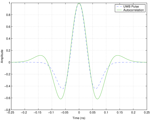
Figure 3: The UWB pulse and the autocorrelation function for $T_{c}=0.25\,$ns.

where $\tau=0.125\,\rm{ns}$ is used (Figure 3).

For the first set of simulations, the timing jitter at the transmitter is modelled by $\mathcal{U}[-25\,{\rm{ps}},25\,{\rm{ps}}]$, where $\mathcal{U}[x,y]$ denotes the uniform distribution on $[x,y]$ [10], [17], and $T_{c}$ is chosen to be $0.25\,{\rm{ns}}$. The total processing gain $N=N_{c}N_{f}$ is taken to be $512$. Also all $10$ users ($N_{u}=10$) are assumed to be sending unit-energy bits ($E_{k}=1$ $\forall k$) and $\sigma_{n}^{2}=0.1$.

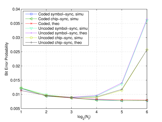
Figure 4: BEP vs $\log_{2}N_{{\rm{f}}}$ for coded and uncoded IR-UWB systems for the AWGN channel case.

Figure 4 shows the BEP of the coded and the uncoded IR-UWB systems for different $N_{f}$ values in an AWGN environment. It is observed that the simulation results match quite closely with the theoretical values. For the coded system, the BEP decreases as $N_{f}$ increases. Since the effect of the MAI on the BEP is asymptotically independent of $N_{f}$, the only effect to consider is that of the timing jitter. Since the effect of the timing jitter is reduced for large $N_{f}$, the plots for the coded system show a decrease in BEP as $N_{f}$ increases. As expected, the performance is the same for the symbol-synchronous and chip-synchronous coded systems. For the uncoded system, there is an optimal value of the processing gain that minimizes the BEP of the system. In this case, there are both the effects of the timing jitter and the MAI. The effect of the timing jitter is mitigated using large $N_{f}$, while that of the MAI is reduced using small $N_{f}$. The optimal value of the processing gains can be approximately calculated using (14) or (18). As expected, the effect of the MAI is larger for the symbol-synchronous system, which causes a larger BEP for such systems compared to the chip-synchronous ones.

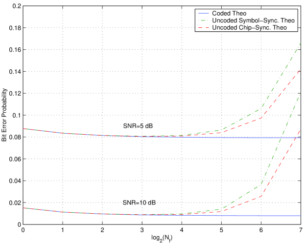
Figure 5: Theoretical BEP vs $\log_{2}N_{{\rm{f}}}$ curves for coded and uncoded IR-UWB systems for different SNR values.

In Figure 5, the BEPs of the coded and uncoded systems are plotted for different signal-to-noise ratios (SNRs). As observed from the figure, as the SNR increases, the trade-off between the processing gains become more significant. This is because, for large SNR, the background noise gets small compared to the noise due to jitter or MAI; hence, the change of processing gain parameters causes significant changes in the BEP of the system due to the effects of timing jitter (and MAI in the uncoded case).

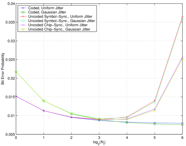
Figure 6: Theoretical BEP vs $\log_{2}N_{{\rm{f}}}$ curves for coded and uncoded IR-UWB systems for uniform and Gaussian jitter statistics.

In Figure 6, the effects of jitter distribution on the system performance are investigated. The BEPs of the coded and uncoded systems are plotted for zero mean uniform [17] and Gaussian [16] timing jitters with the same variance ($208.3$ ps²). From the figure, it is observed that the Gaussian timing jitter increases the BEP more than the uniform timing jitter; i.e. as the timing jitter becomes significant (for small $N_{f}$), the BEP of the system with Gaussian jitter gets larger than that of the system with uniform jitter. The main reason for this difference is that the Gaussian jitter can take significantly large values corresponding to the tail of the distribution, which considerably affects the average BEP of the system.

Now consider a multipath channel with $L=10$ paths, where the fading coefficients are given by $[0.4653\,\,\,\,0.5817\,\,\,\,0.2327-0.4536\,\,\,\,0.3490\,\,\,\,0.2217-0.1163\,\,\,\,0.0233-0.0116-0.0023]$, and the delays by $\tau_{l}=lT_{c}$ for $l=0,\ldots,L-1$, where $T_{c}=0.25\,$ns. The Rake receiver combines all the multipath components using maximal ratio combining (MRC). The jitter is modelled as $\mathcal{U}[-20\,{\rm{ps}},20\,{\rm{ps}}]$, the total processing gain $N$ is equal to $512$, and $\sigma_{n}^{2}=0.01$. There are $10$ users in the system where the first user transmits bits with unit energy ($E_{1}=1$), while the others have $E_{k}=E=5$ $\forall k$.

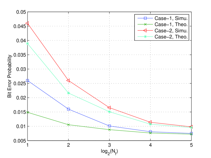
Figure 7: BEP versus $N_{f}$ for coded IR-UWB systems over the multipath channel $[0.4653\,\,0.5817\,\,0.2327-0.4536\,\,0.3490\,\,0.2217-0.1163\,\,0.0233-0.0116-0.0023]$.

Figure 7 plots the BEP of a coded IR-UWB system for a downlink scenario, in which user $1$ is considered as the user of interest and the jitter at the template is as described in Case-1 and Case-2 in Section IV. Note that the theoretical and simulation results get closer as the number of pulses per symbol, $N_{{\rm{f}}}$, increases, as the Gaussian approximation becomes more and more accurate. It is observed that the BEP decreases as $N_{{\rm{f}}}$ increases since the effect of timing jitter is reduced. However, the effect of IFI is not observed since it is negligible compared to the other noise sources. Hence, no significant increase in BEP is observed for larger $N_{f}$, although the IFI increases. Finally, it is observed that the BEPs for Case-1 are smaller than those for Case-2. In other words, the effects of timing jitter are smaller when the jitter is i.i.d. among all the frames and fingers than when it is the same for all the fingers in a given frame and i.i.d. among different frames.

VI Conclusion

The trade-off between the processing gains of an IR system has been investigated in the presence of timing jitter. It has been concluded that, in an AWGN channel, sending more pulses per bit decreases the BEP of a coded system since the effect of the MAI on the BEP is independent of processing gains for a given total processing gain, and the effect of the i.i.d. timing jitter is reduced by sending more pulses. The system performs the same whether the users are symbol-synchronous or chip-synchronous. In an uncoded system, there is a trade-off between $N_{c}$ and $N_{f}$, which reflects the effects of the timing jitter and the MAI. Optimal processing gains can be found by using the approximate closed form expressions for the BEP. It is also concluded that the effect of the MAI is mitigated when the users are chip-synchronous. Therefore, the BEP of a chip-synchronous uncoded system is smaller than that of a symbol-synchronous uncoded system.

For frequency-selective environments, the MAI has no effect on the trade-off between the processing gains of a symbol-synchronous coded system. However, the IFI is mitigated for larger values of $N_{c}$, hence affects the trade-off between the processing gains. Again the effect of the timing jitter is mitigated by increasing $N_{f}$. Therefore, there is a trade-off between the effects of the timing jitter and that of the IFI and the optimal $N_{f}$ ($N_{c}$) value can be chosen by using the approximate BEP expression.

Related to the trade-off study in this paper, investigation of the trade-off between processing gain parameters of a transmitted reference (TR) UWB system [30], [31] remains as an open research problem. Due to the autocorrelation receiver employed in TR UWB systems, the investigation of receiver output statistics would be more challenging in that case.

Acknowledgment: The authors would like to thank Dr. J. Zhang for her support and encouragement.

Appendix A Appendices

A-A Proof of Lemma III.1

Assuming a chip-synchronous system, $a_{m}^{(k)}$ in (6) can be expressed as

$$a_{m}^{(k)}=d_{m}^{(1)}\int w_{{\rm{rx}}}(t-mT_{f}-c_{m}^{(1)}T_{c})\sum_{j=-\infty}^{\infty}d_{j}^{(k)}b^{(k)}_{\lfloor j/N_{f}\rfloor}w_{{\rm{rx}}}(t-jT_{f}-c^{(k)}_{j}T_{c}-\epsilon_{j}^{(k)}-\Delta_{2}^{(k)}T_{c})\,dt,$$ (33)

where $\Delta_{2}^{(k)}\in\{0,1,\ldots,N-1\}$ with equal probability.

Due to random polarity codes $d_{j}^{(k)}$, the distribution of $a_{m}^{(k)}$ is the same for all $\Delta_{2}^{(k)}$ values having the same $\Delta^{(k)}_{1}=\mod\{\Delta_{2}^{(k)},N_{c}\}$ value. Hence, it is sufficient to consider $\Delta_{2}^{(k)}=\Delta_{1}^{(k)}\in\{0,1,...,N_{c}-1\}$. Then, (33) can be expressed as

$$a_{m}^{(k)}=d_{m}^{(1)}\sum_{j=m-1}^{m+1}d_{j}^{(k)}b_{\lfloor j/N_{f}\rfloor}\phi_{w}\left((j-m)T_{f}+(c_{j}^{(k)}-c_{m}^{(1)})T_{c}+\epsilon_{j}^{(k)}+\Delta_{1}^{(k)}T_{c}\right)$$ (34)

From (34), it is observed that $\textrm{E}\{a_{m}^{(k)}\}=0$ due to the independence of polarity codes for different frame and user indices. Also considering the random TH sequences and the polarity codes, it can be shown that

$$\textrm{E}\{(a_{m}^{(k)})^{2}|\Delta_{1}^{(k)}\}=\frac{1}{N_{c}}\left[\textrm{E}\{\phi_{w}^{2}(\epsilon^{(k)})\}+\textrm{E}\{\phi_{w}^{2}(T_{c}-|\epsilon^{(k)}|)\}\right].$$ (35)

Note that $\textrm{E}\{(a_{m}^{(k)})^{2}|\Delta_{1}^{(k)}\}$ is independent of $\Delta_{1}^{(k)}$, which means that the results is true for both the symbol-synchronous and chip-synchronous cases.

Note that $a_{iN_{f}}^{(k)},...,a_{(i+1)N_{f}-1}^{(k)}$ are identically distributed but not independent. However, they form a $1$-dependent sequence [28]. Therefore, for large $N_{f}$ values, $\frac{1}{\sqrt{N_{f}}}\sum_{m=iN_{f}}^{(i+1)N_{f}-1}a_{m}^{(k)}$ converge to a zero mean Gaussian random variable with variance $\textrm{E}\{(a_{iN_{f}}^{(k)})^{2}\}+2\textrm{E}\{a_{iN_{f}}^{(k)}a_{iN_{f}+1}^{(k)}\}$ [28]. It is easy to show that the cross-correlation term is zero using the independence of polarity codes for different indices. Hence, for large $N_{f}$ values, $a^{(k)}$ in (6) is approximately distributed as $a^{(k)}\sim\mathcal{N}(0\,,\,\gamma^{(k)}_{2}N_{f}/N_{c})$, where $\gamma^{(k)}_{2}=\textrm{E}\{\phi_{w}^{2}(\epsilon^{(k)})\}+\textrm{E}\{\phi_{w}^{2}(T_{c}-|\epsilon^{(k)}|)\}$.

A-B Proof of Lemma III.2

Let $p_{m}^{(k)}$ denote the position of the pulse of user $k$ in the $m$th frame ($p_{m}^{(k)}=1,...,N_{c}$). Note that $p_{m}^{(1)}$ denotes the position of the pulse of the template signal in the $m$th frame, assuming user $1$ as the user of interest.

For $p_{m}^{(1)}=2,...,N_{c}-1$, there occurs interference from user $k$ to the $m$th pulse of the template signal if user $k$ has its $m$th pulse at the same position as the $m$th pulse of the template signal or it has its $m$th pulse at a neighboring position to $m$th pulse of the template signal and there is a partial overlap due to the effect of timing jitter. Then $a_{m}^{(k)}$ in (6) can be expressed as

$$a_{m}^{(k)}=b_{i}^{(k)}[\,\phi_{w}(\epsilon_{m}^{(k)})\,I_{\{p_{m}^{(1)}=p_{m}^{(k)}\}}+\phi_{w}(T_{c}-\epsilon_{m}^{(k)})\,I_{\{p_{m}^{(1)}-p_{m}^{(k)}=1\}}I_{\{\epsilon_{m}^{(k)}>0\}}+\phi_{w}(T_{c}+\epsilon_{m}^{(k)})\,I_{\{p_{m}^{(k)}-p_{m}^{(1)}=1\}}I_{\{\epsilon_{m}^{(k)}<0\}}],$$ (36)

where $I_{A}$ denotes an indicator function that is equal to one in $A$ and zero otherwise.

For $p_{m}^{(1)}=1$, we also consider the interference from the previous frame of the signal received from user $k$:

$$a_{m}^{(k)}=b_{i}^{(k)}[\phi_{w}(\epsilon_{m}^{(k)})I_{\{p_{m}^{(k)}=1\}}+\phi_{w}(T_{c}+\epsilon_{m}^{(k)})I_{\{p_{m}^{(k)}=2\}}I_{\{\epsilon_{m}^{(k)}<0\}}]+b_{i}^{(k)}\phi_{w}(T_{c}-\epsilon_{m-1}^{(k)})I_{\{p_{m-1}^{(k)}=N_{c}\}}I_{\{\epsilon_{m-1}^{(k)}>0\}},$$ (37)

for $m=iN_{f}+1,...,(i+1)N_{f}-1$. Note that for $m=iN_{f}$, we just need to replace $b_{i}^{(k)}$ in the third term by $b_{i-1}^{(k)}$ since the previous bit will be in effect in that case.

Similarly, for $p_{m}^{(1)}=N_{c}$,

$$a_{m}^{(k)}=b_{i}^{(k)}[\phi_{w}(\epsilon_{m}^{(k)})I_{\{p_{m}^{(k)}=N_{c}\}}+\phi_{w}(T_{c}-\epsilon_{m}^{(k)})I_{\{p_{m}^{(k)}=N_{c}-1\}}I_{\{\epsilon_{m}^{(k)}>0\}}]+b_{i}^{(k)}\phi_{w}(T_{c}+\epsilon_{m+1}^{(k)})I_{\{p_{m+1}^{(k)}=1\}}I_{\{\epsilon_{m+1}^{(k)}<0\}},$$ (38)

for $m=iN_{f},...,(i+1)N_{f}-2$. For $m=(i+1)N_{f}-1$, $b_{i}^{(k)}$ in the third term is replaced by $b_{i+1}^{(k)}$.

As can be seen from the previous equations, $a_{iN_{f}}^{(k)},...,a_{(i+1)N_{f}-1}^{(k)}$ are not identically distributed due to the possible small difference for the edge values $a_{iN_{f}}^{(k)}$ and $a_{(i+1)N_{f}-1}^{(k)}$ as stated after equations (37) and (38). However, those differences become negligible for large $N_{c}$ and/or $N_{f}$. Then, $a_{iN_{f}}^{(k)},...,a_{(i+1)N_{f}-1}^{(k)}$ can be considered as identically distributed. The mean value can be calculated using $\textrm{E}\{a_{m}^{(k)}|b_{i}^{(k)}\}=\textrm{E}\{\textrm{E}\{a_{m}^{(k)}|\epsilon_{m-1}^{(k)},\epsilon_{m}^{(k)},\epsilon_{m+1}^{(k)},b_{i}^{(k)}\}\}$. From equations (36)-(38), we get

$$\textrm{E}\{a_{m}^{(k)}|\epsilon_{m-1}^{(k)},\epsilon_{m}^{(k)},\epsilon_{m+1}^{(k)},b_{i}^{(k)}\}=\frac{N_{c}-2}{N_{c}^{2}}b_{i}^{(k)}\,[\phi_{w}(\epsilon_{m}^{(k)})+\phi_{w}(T_{c}-\epsilon_{m}^{(k)})\,I_{\{\epsilon_{m}^{(k)}>0\}}+\phi_{w}(T_{c}+\epsilon_{m}^{(k)})\,I_{\{\epsilon_{m}^{(k)}<0\}}]$$

$$+\frac{1}{N_{c}^{2}}b_{i}^{(k)}\,[\phi_{w}(\epsilon_{m}^{(k)})+\phi_{w}(T_{c}+\epsilon_{m}^{(k)})I_{\{\epsilon_{m}^{(k)}<0\}}+\phi_{w}(T_{c}-\epsilon_{m-1}^{(k)})I_{\{\epsilon_{m-1}^{(k)}>0\}}]$$

$$+\frac{1}{N_{c}^{2}}b_{i}^{(k)}\,[\phi_{w}(\epsilon_{m}^{(k)})+\phi_{w}(T_{c}-\epsilon_{m}^{(k)})I_{\{\epsilon_{m}^{(k)}>0\}}+\phi_{w}(T_{c}+\epsilon_{m+1}^{(k)})I_{\{\epsilon_{m+1}^{(k)}<0\}}],$$ (39)

for $m=iN_{f},...,(i+1)N_{f}-1$. Then, taking expectation with respect to timing jitters, we get

$$\textrm{E}\{a_{m}^{(k)}|b_{i}^{(k)}\}=b_{i}^{(k)}\gamma^{(k)}_{1}/N_{c},$$ (40)

where $\gamma^{(k)}_{1}=\textrm{E}\{\phi_{w}(\epsilon_{m}^{(k)})\}+\textrm{E}\{\phi_{w}(T_{c}-|\epsilon_{m}^{(k)}|)\}$.

By similar calculations, it can be shown that

$$\textrm{E}\{(a_{m}^{(k)})^{2}|b_{i}^{(k)}\} =\frac{\gamma^{(k)}_{2}}{N_{c}}+\frac{2}{N_{c}^{3}}\textrm{E}\{\phi_{w}(\epsilon^{(k)})\}\textrm{E}\{\phi_{w}(T_{c}-|\epsilon^{(k)}|)\}$$

$$+\frac{4}{N_{c}^{3}}\int_{-\infty}^{0}\phi_{w}(T_{c}+\epsilon^{(k)})p(\epsilon^{(k)})d\epsilon^{(k)}\int_{0}^{\infty}\phi_{w}(T_{c}-\epsilon^{(k)})p(\epsilon^{(k)})d\epsilon^{(k)},$$ (41)

where $p(\epsilon^{(k)})$ is the probability density function of i.i.d. timing jitters for user $k$ and $\gamma^{(k)}_{2}=\textrm{E}\{\phi_{w}^{2}(\epsilon_{m}^{(k)})\}+\textrm{E}\{\phi_{w}^{2}(T_{c}-|\epsilon_{m}^{(k)}|)\}$. Note that frame indices are omitted in the last equation since the results do not depend on them.

The cross-correlations between consecutive values of the 1-dependent sequence $a_{iN_{f}}^{(k)},...,a_{(i+1)N_{f}-1}^{(k)}$ can be obtained as

$$\textrm{E}\{a_{m}^{(k)}a_{m+1}^{(k)}|b_{i}^{(k)}\} =(\gamma^{(k)}_{1})^{2}/N_{c}^{2}-\frac{1}{N_{c}^{3}}\gamma^{(k)}_{1}\textrm{E}\{\phi_{w}(T_{c}-|\epsilon^{(k)}|)\}$$

$$+\frac{1}{N_{c}^{3}}\textrm{E}\{\phi_{w}(T_{c}-|\epsilon^{(k)}|)\phi_{w}(\epsilon^{(k)})\}+\frac{1}{N_{c}^{4}}(\textrm{E}\{\phi_{w}(T_{c}-|\epsilon^{(k)}|)\})^{2}.$$ (42)

Then, invoking the theorem for 1-dependent sequences [28] and using (40)-(A-B), the sum of interferences to each pulse of the template, $\sum_{m=iN_{f}}^{(i+1)N_{f}-1}a_{m}^{(k)}|b_{i}^{(k)}$, is approximately distributed as in (10), where $\gamma^{(k)}_{1}$, $\gamma^{(k)}_{2}$, $\beta^{(k)}_{1}$ and $\beta^{(k)}_{2}$ are as in (III.2).

A-C Proof of Lemma IV.1

In order to calculate the distribution of $\hat{a}=\sqrt{\frac{E_{1}}{N_{f}}}\sum_{m=iN_{f}}^{(i+1)N_{f}-1}\hat{a}_{m}$, consider $\hat{a}_{m}$ given by (24). From (24), it can be observed that $\textrm{E}\{\hat{a}_{m}\}=0$ due to the random polarity codes. To calculate $\textrm{E}\{\hat{a}_{m}^{2}\}$, we first condition on the timing jitter values:

$$\textrm{E}\{\hat{a}_{m}^{2}|\epsilon^{(1)}_{m-1},\epsilon^{(1)}_{m+1},\hat{\boldsymbol{\epsilon}}_{m}\} =\frac{1}{N_{c}^{2}}\sum_{i=0}^{N_{c}-1}\sum_{l=0}^{N_{c}-1}\left[\phi_{uv}^{(m)}\left((l-i-N_{c})T_{c}+\epsilon_{m-1}^{(1)}\right)\right]^{2}$$

$$+\frac{1}{N_{c}^{2}}\sum_{i=0}^{N_{c}-1}\sum_{k=0}^{N_{c}-1}\left[\phi_{uv}^{(m)}\left((k-i+N_{c})T_{c}+\epsilon_{m+1}^{(1)}\right)\right]^{2}$$

$$=\frac{1}{N_{c}^{2}}\sum_{j=1}^{M}j\left\{\left[\phi_{uv}^{(m)}(jT_{c}+\epsilon_{m+1}^{(1)})\right]^{2}+\left[\phi_{uv}^{(m)}(-jT_{c}+\epsilon_{m-1}^{(1)})\right]^{2}\right\},$$ (43)

where we use the fact that the time-hopping sequences are uniformly distributed in $\{0,1,\ldots,N_{c}-1\}$, and $\hat{\boldsymbol{\epsilon}}_{m}=[\hat{\epsilon}_{m,0}\cdots\hat{\epsilon}_{m,L-1}]$. Then, averaging over the distribution of the timing jitters, we get

$$\textrm{E}\{\hat{a}_{m}^{2}\}=\frac{1}{N_{c}^{2}}\sum_{j=1}^{M}j\left\{\textrm{E}\{[\phi_{uv}^{(m)}(jT_{c}+\epsilon_{m+1}^{(1)})]^{2}\}+\textrm{E}\{[\phi_{uv}^{(m)}(-jT_{c}+\epsilon_{m-1}^{(1)})]^{2}\}\right\}.$$ (44)

From (24), it is observed that $\textrm{E}\{\hat{a}_{m}\hat{a}_{n}\}=0$ for $|m-n|>1$ and $\textrm{E}\{\hat{a}_{m}\hat{a}_{m+1}\}$ can be expressed as

$$\textrm{E}\{\hat{a}_{m}\hat{a}_{m+1}\}=\frac{1}{N_{c}^{2}}\sum_{j=1}^{M}j\,\textrm{E}\{\phi_{uv}^{(m)}(jT_{c}+\epsilon_{m}^{(1)})\phi_{uv}^{(m)}(-jT_{c}+\epsilon_{m+1}^{(1)})\}.$$ (45)

Since $\frac{1}{\sqrt{N_{f}}}\sum_{m=iN_{f}}^{(i+1)N_{f}-1}\hat{a}_{m}$ converges to $\mathcal{N}\left(0\,,\,\textrm{E}\{\hat{a}_{m}^{2}\}+2\textrm{E}\{\hat{a}_{m}\hat{a}_{m+1}\}\right)$ as $N_{f}\longrightarrow\infty$ [28], we can obtain (25) from (44) and (45).

A-D Proof of Lemma IV.2

The aim is to calculate the asymptotic distribution of $a^{(k)}=\sum_{m=iN_{f}}^{(i+1)N_{f}-1}a_{m}^{(k)}$, where $a_{m}^{(k)}$ is given by (27).

From (27), it can be observed that $\textrm{E}\{a_{m}^{(k)}\}=0$ due to the random polarity codes. In order to calculate the variance, we first condition on the jitter values:

$$\textrm{E}\{(a_{m}^{(k)})^{2} |\epsilon^{(k)}_{m-1},\epsilon^{(k)}_{m},\epsilon^{(k)}_{m+1},\hat{\boldsymbol{\epsilon}}_{m}\}=\frac{1}{N_{c}^{2}}\sum_{i=0}^{N_{c}-1}\{\sum_{j=0}^{N_{c}-1}\left[\phi_{uv}^{(m)}\left((j-i-N_{c})T_{c}+\epsilon_{m-1}^{(k)}\right)\right]^{2}$$

$$+\sum_{k=0}^{N_{c}-1}\left[\phi_{uv}^{(m)}\left((k-i)T_{c}+\epsilon_{m}^{(k)}\right)\right]^{2}+\sum_{l=0}^{N_{c}-1}\left[\phi_{uv}^{(m)}\left((l-i+N_{c})T_{c}+\epsilon_{m+1}^{(k)}\right)\right]^{2}\},$$ (46)

where use the fact that the time-hopping sequences are uniformly distributed in $\{0,1,\ldots,N_{c}-1\}$ and $\hat{\boldsymbol{\epsilon}}_{m}=[\hat{\epsilon}_{m,0}\cdots\hat{\epsilon}_{m,L-1}]$. Then, averaging over jitter statistics, we obtain, $\textrm{E}\{(a_{m}^{(k)})^{2}\}=\frac{1}{N_{c}}\sum_{j=-M}^{M}\textrm{E}\{[\phi_{uv}^{(m)}(jT_{c}+\epsilon^{(k)})]^{2}\}$.

Also it can be observed that $\textrm{E}\{a_{m}^{(k)}a_{n}^{(k)}\}=0$ for $m\neq n$ due to the independence of polarity codes.

All in all, $\frac{1}{\sqrt{N_{f}}}\sum_{m=iN_{f}}^{(i+1)N_{f}-1}a_{m}^{(k)}$ converges to $\frac{1}{N_{c}}\sum_{j=-M}^{M}\textrm{E}\{[\phi_{uv}^{(m)}(jT_{c}+\epsilon^{(k)})]^{2}\}$ as $N_{f}\longrightarrow\infty$ [28], from which the result of Lemma IV.2 follows.

Sinan Gezici received the B.S. degree from Bilkent University, Turkey in 2001, and the Ph.D. degree in Electrical Engineering from Princeton University in 2006. From April 2006 to January 2007, he worked as a Visiting Member of Technical Staff at Mitsubishi Electric Research Laboratories, Cambridge, MA. Since February 2007, he has been an Assistant Professor in the Department of Electrical and Electronics Engineering at Bilkent University.

Dr. Gezici’s research interests are in the areas of signal detection, estimation and optimization theory, and their applications to wireless communications and localization systems. Currently, he has a particular interest in ultra-wideband systems for communications and sensing applications.

Andreas F. Molisch (S’89, M’95, SM’00, F’05) received the Dipl. Ing., Dr. techn., and habilitation degrees from the Technical University Vienna (Austria) in 1990, 1994, and 1999, respectively. From 1991 to 2000, he was with the TU Vienna, becoming an associate professor there in 1999. From 2000-2002, he was with the Wireless Systems Research Department at AT&T (Bell) Laboratories Research in Middletown, NJ. Since then, he has been with Mitsubishi Electric Research Labs, Cambridge, MA, where he is now a Distinguished Member of Technical Staff. He is also professor and chairholder for radio systems at Lund University, Sweden.

Dr. Molisch has done research in the areas of SAW filters, radiative transfer in atomic vapors, atomic line filters, smart antennas, and wideband systems. His current research interests are measurement and modeling of mobile radio channels, UWB, cooperative communications, and MIMO systems. Dr. Molisch has authored, co-authored or edited four books (among them the recent textbook “Wireless Communications,” Wiley-IEEE Press), eleven book chapters, some 95 journal papers, and numerous conference contributions.

Dr. Molisch is an editor of the IEEE Trans. Wireless Comm., co-editor of recent special issues on MIMO and smart antennas (in J. Wireless Comm. Mob. Comp.), and UWB (in IEEE - JSAC). He has been member of numerous TPCs, vice chair of the TPC of VTC 2005 spring, general chair of ICUWB 2006, and TPC co-chair of the wireless symposium of Globecomm 2007. He has participated in the European research initiatives “COST 231”, “COST 259”, and “COST273”, where he was chairman of the MIMO channel working group, he was chairman of the IEEE 802.15.4a channel model standardization group, and is also chairman of Commission C (signals and systems) of URSI (International Union of Radio Scientists). Dr. Molisch is a Fellow of the IEEE and recipient of several awards.

H. Vincent Poor (S’72, M’77, SM’82, F’77) received the Ph.D. degree in EECS from Princeton University in 1977. From 1977 until 1990, he was on the faculty of the University of Illinois at Urbana-Champaign. Since 1990 he has been on the faculty at Princeton, where he is the Michael Henry Strater University Professor of Electrical Engineering and Dean of the School of Engineering and Applied Science. Dr. Poor’s research interests are in the areas of stochastic analysis, statistical signal processing and their applications in wireless networks and related fields. Among his publications in these areas is the recent book MIMO Wireless Communications (Cambridge University Press, 2007).

Dr. Poor is a member of the National Academy of Engineering and is a Fellow of the American Academy of Arts and Sciences. He is also a Fellow of the Institute of Mathematical Statistics, the Optical Society of America, and other organizations. In 1990, he served as President of the IEEE Information Theory Society, and in 2004-2007 he served as the Editor-in-Chief of the IEEE Transactions on Information Theory. Recent recognition of his work includes a Guggenheim Fellowship and the IEEE Education Medal.

Hisashi Kobayashi is the Sherman Fairchild University Professor of Electrical Engineering and Computer Science at Princeton University since 1986, when he joined the Princeton faculty as the Dean of the School of Engineering and Applied Science (1986-91). From 1967 till 1982 he was with the IBM Research Center in Yorktown Heights, and from 1982 to 1986 he served as the founding Director of the IBM Tokyo Research Laboratory. His research experiences include radar systems, high speed data transmission, coding for high density digital recording, image compression algorithms, performance modeling and analysis of computers and communication systems. His current research activities are on performance modeling and analysis of high speed networks, wireless communications and geolocation algorithms, network security, and teletraffic & queuing theory. He published “Modeling and Analysis” (Addison-Wesley, 1978), and is authoring a new book with B. L. Mark entitled “Probability, Statistics and Stochastic Modeling: Foundations of System Performance Evaluation” (Prentice Hall, 2005). He is a member of the Engineering Academy of Japan, a Life Fellow of IEEE, and a Fellow of IEICE of Japan. He was the recipient of the Humboldt Prize from Germany (1979), the IFIP’s Silver Core Award (1981), and two IBM Outstanding Contribution Awards. He received his Ph.D. degree (1967) from Princeton University and BE and ME degrees (1961, 63) from the University of Tokyo, all in Electrical Engineering.

References

• [1] Federal Communications Commission, β€œFCC 00-163: Notice of Proposed Rule Making,” May 2000.
• [2] Federal Communications Commission, β€œFCC 02-48: First Report and Order,” Feb. 2002.
• [3] M. Z. Win and R. A. Scholtz, β€œImpulse radio: How it works,” IEEE Communications Letters, 2(2):36-38, Feb. 1998.
• [4] M. Z. Win, R. A. Scholtz, and L. W. Fullerton, β€œTime-hopping SSMA techniques for impulse radio with an analog modulated data subcarrier,” Proc. IEEE Fourth Int. Symp. on Spread Spectrum Techniques & Applications, pp. 359-364, Mainz, Germany, Sept. 1996.
• [5] M. Z. Win and R. A. Scholtz, ”Ultra-wide bandwidth time-hopping spread-spectrum impulse radio for wireless multiple-access communications,” IEEE Trans. Commun., vol. 48, no. 4, pp. 679-691, Apr. 2000.
• [6] S. Gezici, Z. Tian, G. B. Giannakis, H. Kobayashi, A. F. Molisch, H. V. Poor, and Z. Sahinoglu, β€œLocalization via ultra-wideband radios,” IEEE Signal Processing Magazine (Special Issue on Signal Processing for Positioning and Navigation with Applications to Communications), vol. 22, issue 4, pp. 70-84, July 2005.
• [7] W. Suwansantisuk and M. Z. Win, β€œMultipath aided rapid acquisition: Optimal search strategies,” IEEE Transactions on Information Theory, vol. 52, no. 1, pp. 174-193, Jan. 2007.
• [8] E. Fishler and H. V. Poor, β€œOn the tradeoff between two types of processing gain,” Proc. 40th Annual Allerton Conference on Communication, Control, and Computing, Monticello, IL, Oct.2-4, 2002.
• [9] A. F. Molisch, J. Zhang, and M. Miyake, β€œTime hopping and frequency hopping in ultrawideband systems,” Proc. IEEE Pacific Rim Conference on Communications, Computers and Signal Processing (PACRIM 2003), Victoria, Canada, August 28-30, 2003.
• [10] I. Guvenc and H. Arslan, β€œPerformance evaluation of UWB systems in the presence of timing jitter,” IEEE Conference on Ultra Wideband Systems and Technologies (UWBST 2003), pp. 136-141, Reston, VA, Nov. 16-19, 2003.
• [11] M. Z. Win, β€œA unified spectral analysis of generalized time-hopping spread-spectrum signals in the presence of timing jitter,” IEEE Journal on Selected Areas in Communications, vol. 20, no. 9, pp. 1664-1676, Dec. 2002.
• [12] W. M. Lovelace and J. K. Townsend, β€œThe effects of timing jitter and tracking on the performance of impulse radio,” IEEE Journal on Selected Areas in Communications, vol. 20, no. 9, pp. 1646-1651, Dec. 2002.
• [13] Y.-P. Nakache and A. F. Molisch, β€œSpectral shape of UWB signals influence of modulation format, multiple access scheme and pulse shape,” Proc. IEEE Vehicular Technology Conference, (VTC 2003-Spring), vol. 4, pp. 2510-2514, Jeju, Korea, April 2003.
• [14] C. J. Le-Martret and G. B. Giannakis, β€œAll-digital PAM impulse radio for multiple-access through frequency-selective multipath,” Proc. IEEE Global Telecommunications Conference (GLOBECOM2000), vol. 1, pp. 77-81, San Fransisco, CA, Nov. 2000.
• [15] B. Sadler and A. Swami, β€œOn the performance of UWB and DS-spread spectrum communications systems,” Proc. IEEE Conference of Ultra Wideband Systems and Technologies (UWBST’02), pp. 289-292, Baltimore, MD, May 2002.
• [16] N. V. Kokkalis, P. T. Mathiopoulos, G. K. Karagiannidis, and C. S. Koukourlis, β€œPerformance analysis of M-ary PPM TH-UWB systems in the presence of MUI and timing jitter,” IEEE Journal on Selected Areas in Communications, vol. 24, issue 4, Part 1, pp. 822-828, April 2006.
• [17] W. Zhang, Z. Bai, H. Shen, W. Liu, K. S. Kwak; β€œA novel timing jitter resist method in UWB systems,” IEEE International Symposium on Communications and Information Technology (ISCIT 2005), vol. 2, pp. 833-836, Oct. 12-14, 2005.
• [18] S. Gezici, H. Kobayashi, H. V. Poor and A. F. Molisch, β€œPerformance evaluation of impulse radio UWB systems with pulse-based polarity randomization,” IEEE Transactions on Signal Processing, vol. 53, no. 7, pp. 1-13, July 2005.
• [19] S. VerdΓΊ. Multiuser Detection, Cambridge University Press, Cambridge, UK, 1998.
• [20] J. Foerster, Ed., β€œChannel modeling sub-committee report final,” IEEE, Document IEEE P802.15-02/490r1-SG3a, 2003.
• [21] M. Z. Win and R. A. Scholtz, β€œCharacterization of ultra-wide bandwidth wireless indoor channels: a communication-theoretic view,” IEEE Journal on Selected Areas in Communications, vol. 20, issue 9, pp. 1613-1627, Dec. 2002.
• [22] D. Cassioli, M. Z. Win, F. Vatalaro and A. F. Molisch, β€œPerformance of low-complexity Rake reception in a realistic UWB channel,” Proceedings of the IEEE International Conference on Communications, 2002 (ICC 2002), vol. 2, pp. 763-767, New York, NY, April 28-May 2, 2002.
• [23] M. Z. Win and R. A. Scholtz, β€œOn the energy capture of ultra-wide bandwidth signals in dense multipath environments,” IEEE Communications Letters, vol. 2, no. 9, pp. 245-247, Sept. 1998.
• [24] M. Z. Win and R. A. Scholtz, β€œOn the robustness of ultra-wide bandwidth signals in dense multipath environments,” IEEE Communications Letters, vol. 2, no. 2, pp. 51-53, Feb. 1998.
• [25] M. Z. Win and Z. A. Kostic, β€œVirtual path analysis of selective Rake receiver in dense multipath channels,” IEEE Communications Letters, vol. 3, no. 11, pp. 308-310, Nov. 1999.
• [26] M. Z. Win and Z. A. Kostic, β€œImpact of spreading bandwidth on Rake reception in dense multipath channels,” IEEE Journal on Selected Areas in Communications, vol. 17, no. 10, pp. 1794-1806, Oct. 1999.
• [27] M. Z. Win, G. Chrisikos, and N. R. Sollenberger, β€œPerformance of Rake reception in dense multipath channels: Implications of spreading bandwidth and selection diversity order,” IEEE Journal on Selected Areas in Communications, vol. 18, no. 8, pp. 1516-1525, Aug. 2000.
• [28] P. Bilingsley, Probability and Measure, John Wiley & Sons, New York, 2nd edition, 1986.
• [29] F. Ramirez-Mireles and R. A. Scholtz, β€œMultiple-access performance limits with time hopping and pulse-position modulation,” Proc. IEEE Military Communications Conference (MILCOM’98), vol. 2, Oct. 1998, pp. 529-533.
• [30] T. Q. S. Quek and M. Z. Win, β€œAnalysis of UWB transmitted-reference communication systems in dense multipath channels,” IEEE Journal on Selected Areas in Communications, vol. 23, no. 9, pp. 1863-1874, Sept. 2005.
• [31] R. Hoctor and H. Tomlinson, β€œDelay-hopped transmitted-reference RF communications,” Proceedings of the IEEE Conference of Ultra Wideband Systems and Technologies 2002 (UWBST’02), pp. 265-269, Baltimore, MD, May 2002.