Sparticle Spectra and LHC Signatures for Large Volume String Compactifications
Abstract:
We study the supersymmetric particle spectra and LHC collider observables for the large-volume string models with a fundamental scale of that arise in moduli-fixed string compactifications with branes and fluxes. The presence of magnetic fluxes on the brane world volume, required for chirality, perturb the soft terms away from those previously computed in the dilute-flux limit. We use the difference in high-scale gauge couplings to estimate the magnitude of this perturbation and study the potential effects of the magnetic fluxes by generating many random spectra with the soft terms perturbed around the dilute flux limit. Even with a variation in the high-scale soft terms the low-energy spectra take a clear and predictive form. The resulting spectra are broadly similar to those arising on the SPS1a slope, but more degenerate. In their minimal version the models predict the ratios of gaugino masses to be , different to both mSUGRA and mirage mediation. Among the scalars, the squarks tend to be lighter and the sleptons heavier than for comparable mSUGRA models. We generate of sample LHC data for the random spectra in order to study the range of collider phenomenology that can occur. We perform a detailed mass reconstruction on one example large-volume string model spectrum. of integrated luminosity is sufficient to discriminate the model from mSUGRA and aspects of the sparticle spectrum can be accurately reconstructed.
1 Introduction
The imminent advent of the Large Hadron Collider (LHC) is an excellent motivation to develop techniques to relate high energy string compactifications to observable low-energy collider physics. The LHC will be an unprecedented probe of the terascale and of the physics that stabilises the electroweak hierarchy. If supersymmetry is discovered at the LHC, it will be necessary to connect the collider observables and the spectrum of superparticles to a more fundamental theory such as string theory.
Supersymmetric phenomenology is the study not of supersymmetry but of supersymmetry breaking: the undetermined parameters of the minimal supersymmetric standard model (MSSM) are those associated with the soft supersymmetry breaking terms, such as gaugino masses, scalar masses or trilinear A-terms. There are over one hundred such parameters in a general phenomenological parameterisation of the MSSM. The many different possibilities for supersymmetric phenomenology are determined by the many different possibilities for the soft terms. However, high scale constructions such as string compactifications contain far fewer independent parameters and so could be expected to lead to distinctive patterns of soft terms.
Broken supersymmetry is a property of the vacuum of the theory. The study of supersymmetry breaking vacua in string theory therefore requires control over both the moduli potential and the quantum corrections that enter into it. The quantum corrections play a crucial role for the large-volume models [1, 2] that we study here. The first constructions of IIB string models with all moduli stabilised [3] involved unbroken supersymmetry, which had to be broken by hand by the addition of -branes, with a gravitino mass that could only be lowered below the Planck scale by fine-tuning. It was subsequently realised that with the inclusion of quantum corrections [4] the moduli potential can admit non-supersymmetric minima [5] and even naturally generate a hierarchically small supersymmetry-breaking scale [1, 2]. This is the large volume scenario that we will explore here.111The possibility of generating low-scale supersymmetry breaking from the moduli-stabilising potential has also been studied in corners of string theory different from that of IIB with fluxes [6].
Nonetheless, it is still a long way from the mere existence of low-scale supersymmetry breaking to actual phenomenology, and turning any given string compactification into LHC collider observables requires many steps. We will assume gravity-mediated supersymmetry breaking as the most directly motivated scenario from string compactifications; the modifications for other proposals are straightforward.
-
1.
The first requirement is that the compactification moduli be stabilised within a controlled approximation. This is necessary to ensure that the compactification is a good vacuum solution of string theory.
-
2.
The second requirement is that supersymmetry is broken in the vacuum, so that soft terms can be generated. We also require the supersymmetry breaking to be hierarchically small, in order that the soft terms appear at the TeV scale rather than near the Planck scale.
-
3.
The third requirement is a visible sector containing the Standard Model gauge group, with an understanding of the non-renormalisable couplings between the visible sector and the hidden sector moduli that break supersymmetry.
-
4.
The fourth task is to combine these couplings with the hidden sector supersymmetry breaking to compute the visible sector soft supersymmetry breaking terms at the high-energy compactification scale. Here we also would like an understanding of why the soft terms generated do not lead to large CP violation or flavour-changing neutral currents.
-
5.
The fifth task is to run these soft terms down to the TeV-scale, in order to compute the physical sparticle spectrum.
- 6.
-
7.
Finally, we also want an estimate of the uncertainties arising from the above six steps.
The aim of this paper is to carry out this program almost in its entirety for a specific and well-motivated class of string compactifications, the large volume models developed in ref. [1].222The omission is in the lack of an explicit magnetised brane configuration realising the MSSM gauge group; this we simply assume can be achieved. These models arise within IIB flux compactifications with moduli stabilisation and are characterised by broken supersymmetry with an exponentially large compactification volume. This allows the natural generation of hierarchies between mass scales, an extremely desirable feature. The large volume lowers both the string scale and the gravitino mass with respect to the Planck scale ,
| (1) |
refers to a dimensionless quantity: the volume measured in powers of the string-length . The dimensionful volume of the compactification manifold is . From (1), an intermediate string scale gives rise to TeV-scale supersymmetry breaking. The phenomenological implications of these models have been studied in [1, 2, 10, 11, 12] where requirements 1-5 above have been addressed. In this article we will first review the most relevant results from those references and complete requirements 6 and 7 above in order to make direct contact with potential observables at the LHC.
The organisation of this paper is as follows. In section 2 we review the large-volume models and the moduli stabilisation that generates the exponentially large volume. We also describe the computation of soft terms and explain why leading order flavour universality is assured, summarising the results of refs. [1, 2, 13, 12]. We also describe how magnetic fluxes perturb the soft terms away from those computed in the dilute-flux limit. We estimate the magnitude of the flux perturbation from the non-universality of the high-scale gauge couplings. Such corrections will generate an uncertainty in the high-scale soft terms that will translate into an uncertainty in the low-energy spectra and observables. In section 3 we examine the low-energy spectra arising from the soft terms considered in section 2.3, by generating random soft terms perturbed about the dilute-flux limit. We describe the generic properties of the resulting low-energy spectra and compare with those arising in mSUGRA or mirage mediation models. In section 4 we study collider observables for these spectra. We use counting observables to scan the properties of the randomly generated spectra, and show that for a sample spectrum sparticle masses can be reconstructed. In section 5 we present our conclusions.
We have made an effort to make this article self-contained. A phenomenologically minded reader may wish to skip the formal details of section 2 and start in section 2.3.
2 Large-Volume Models
Large-volume models represent a class of string compactifications, with all moduli stabilised, in which quantum corrections to the scalar potential naturally lead to a exponentially large volume. They were first found in references [1, 2]. They are robust against additional quantum corrections, such as those of [14, 15]. A recent detailed study of this robustness is [16]. They have been applied to obtain string theory inflation [17], natural QCD axions [18], the scale for neutrino masses [19] and to low energy supersymmetric phenomenology [10, 11, 13, 12] in which they provide a natural hierarchy for supersymmetry breaking with the large volume leading to an intermediate string scale. A comprehensive review is [20]. We start by reviewing their construction and properties.
2.1 Construction
These models arise as a rather generic limit of flux compactifications of IIB string theory in the presence of D3 and D7 branes. In supersymmetric IIB compactifications the Kähler potential and superpotential for the moduli take the standard form [3, 21, 4, 22],
| (2) | |||||
| (3) |
where the dependence on the complex structure moduli is encoded in the Calabi-Yau form . corresponds to the three-form fluxes and is linear in the dilaton . We have included the leading correction to the Kähler potential, which depends on with the Euler number of the Calabi-Yau manifold . Large-volume models require to have at least two Kähler moduli , one of which is a blow-up mode, as well as a negative Euler number, i.e. . The simplest model is that of , which we use as our working example. For this the volume can be written as [1, 23]
| (4) |
and denote big and small cycles. The geometry is analogous to that of a Swiss cheese: the cycle controls the volume (‘the size of the cheese’) and controls a blow-up cycle (‘the size of the hole’).
The moduli scalar potential is
| (5) |
where . Dropping terms sub-leading in , this potential becomes
| (6) |
in the limit , where are numerical constants. The first terms of (6) stabilise the dilaton and complex structure moduli at . The remaining terms stabilise the Kähler moduli. The non-perturbative terms in balance against the perturbative corrections in the volume, and it can be shown that at the minimum of the scalar potential [1]
where is the value of the flux superpotential at the minimum of and fields, and is a numerical constant. The resulting volume is exponentially large with a small blow-up cycle. This geometry is shown in figure 1.
The minimum avoids two problems of the KKLT scenario. First, as its consistency does not require a fine-tuning of , its existence is more generic. Secondly, the stabilisation of the moduli can never destabilise the moduli, as near the minimum the relevant terms in (6) come with different powers of the volume. A phenomenological advantage is that this minimum also breaks supersymmetry and generates an exponentially large volume.333The minimum of the potential (6) is at negative vacuum energy with supersymmetry broken. Just as in KKLT a lifting term is desirable to obtain de Sitter or Minkowski space. There are several possible sources for this lifting term [24] (see [25] for a recent detailed analysis for KKLT and large volume models). Since the anti de Sitter minimum is already non supersymmetric, in contrast to KKLT models, the contribution of this lifting term to the soft breaking terms is suppressed and does not play an important role in the rest of this paper.
This large volume allows the generation of hierarchies by lowering both the string scale and gravitino mass as in (1). A volume is required to explain the weak/Planck hierarchy and give TeV-scale supersymmetry breaking. We assume such a volume throughout this paper. Further attractive features are that the volume also gives an axion decay constant in the allowed window [18] and the required neutrino suppression scale of [19].
A fully realistic model must have a Standard Model sector, which requires an appropriate configuration of O-planes and magnetised D7-branes. Chirality arises from the topological intersection numbers of differently magnetised branes.444Magnetic flux on D7 branes is equivalent to dissolved D5 branes. The chirality arises from the point like intersection of the dissolved D5 branes. To avoid having gauge groups that are too weakly coupled, we must wrap the Standard Model D7 branes on the small cycle corresponding to . As the branes should wrap a blow-up cycle, the brane configuration will represent a local construction of the Standard Model. We assume such a configuration can be found, but do not attempt to realise the brane configuration explicitly. The techniques involved in explicitly constructing such a configuration will be similar to those used in models of branes at singularities. In this context there has been recent effort at constructing MSSM-like gauge groups - see [26, 27, 28] for progress.
As , the infrared physics of these models is that of the MSSM. The computation of the soft terms is then central to the study of the low energy phenomenology.
2.2 Gauge Couplings
The gauge kinetic functions are principally determined by the cycles wrapped by the D7 branes. If is the Kähler modulus corresponding to a particular 4-cycle, reduction of the DBI action for an unmagnetised brane wrapped on that cycle gives555This holds with the phenomenology conventions ; with conventions the gauge kinetic function is .
| (7) |
To generate chirality we require the branes to be magnetised. The magnetic fluxes alter (7) to
| (8) |
where is a topological function of the fluxes present on the brane. This can be understood microscopically. The gauge coupling is given by an integral over the cycle wrapped by the brane,
| (9) |
Thus in the presence of flux, the gauge coupling depends on the magnetic flux as well as the cycle volume.666In computing explicit expressions for the factors , it is easiest to use the Chern-Simons action to get the correction to , and then use holomorphy for the correction to . The factors have been explicitly computed for toroidal orientifolds [29, 30].
As a minimal scenario we assume that the Standard Model branes live on a single blow-up cycle and so the gauge kinetic functions depend upon only one Kähler modulus . As the cycle size is increased, the magnetic fluxes are diluted and their contribution to the gauge couplings goes away. It is useful to consider this dilute flux limit in addition to the physical case, and to see the latter as a perturbation on the former. The Standard Model gauge kinetic functions will be
-
1.
Dilute flux limit
(10) -
2.
Physical case
(11) (12) (13)
The factor accounts for the uncertainty in normalising the gauge field: the that appears in intersecting brane models in general has a different normalisation to that of . The ‘canonical’ value only holds for grand unified models; in general, is model dependent. Typically in D-brane models hypercharge is an anomaly free linear combination of different ’s coming from different factors, the particular linear combination determining the value of the normalisation factor . The functions depend on the microscopic configuration of branes and fluxes, and we also regard these as unknown.
2.3 Soft Breaking Terms
A four dimensional supergravity Lagrangian is specified at two space-time derivatives by the Kähler potential , superpotential and gauge kinetic function . The computation of soft terms starts by expanding these as a power series in the matter fields,
| (14) | |||||
| (15) | |||||
| (16) |
Here denotes a generic modulus field and a generic matter field. In the MSSM the and terms apply only to the Higgs fields and so for these we have written and explicitly. Gravity-mediated supersymmetry breaking is then quantified through the moduli F-terms, given by
| (17) |
The relationships of the expansions (14) to (16) to the soft supersymmetry breaking terms are given in full detail in ref. [31].
2.3.1 Gaugino Masses
The canonically normalised gaugino masses are given by
| (18) |
The gaugino masses that follow from (8) are
-
1.
Dilute flux limit
(19) -
2.
Physical case
(20)
where we write for , and similarly for and .
In the limit of large cycle volume, the flux becomes dilute and the gaugino masses become universal at the compactification scale where the soft parameters are computed. In the physical case, the gaugino masses are non-universal due to the flux contribution. However for non-abelian gauge groups - i.e. for the wino and gluino - it follows from (11) and (12) that the fractional non-universality of gaugino masses is identical to that of the gauge couplings:
| (21) |
Due to the factor in the gauge couplings, this relation does not hold for . Here we have
| (22) |
where is the unknown normalisation factor.
2.3.2 Scalar Soft Terms
For the case of diagonal matter field metrics, (no summation over ), the scalar masses, A-terms and B-term are given by [31]
| (23) | |||||
| (24) | |||||
| (25) | |||||
As mentioned above, the tree-level vacuum energy (in Planck units) is much smaller than () and thus the effects of uplifting can be neglected. To compute the scalar masses and A-terms, the key piece of information required is the modular dependence of the kinetic terms . In the dilute flux limit this can be derived by relating the modular scaling of to that of the physical Yukawa couplings through the relation
| (26) |
and the fact that the moduli cannot appear perturbatively in due to the combination of holomorphy and the Peccei-Quinn (PQ) shift symmetry. Ref. [13] used this reasoning to derive
| (27) |
where refers to the complex structure moduli. In the dilute flux limit this leads to scalar masses and A-terms given by
| (28) | |||||
| (29) |
The superpotential -term can be shown to vanish due to scaling arguments [13]: in the limit that , any non-zero superpotential -term would generate a mass for the Higgs field above the string scale. A non fine-tuned (i.e. weak-scale) term can be generated through the Giudice-Masiero mechanism [32], and as such is guaranteed to be of a similar order to the other soft terms. In fact it turns out to be difficult to satisfy the B-term constraint (29) when running to low energies. However, the Higgs sector is by far the least understood sector of the Standard Model. As such it may be non-minimal, or the B-term may receive an extra contribution through the vacuum expectation value of a gauge-invariant scalar, . In this paper we therefore follow normal phenomenological practice by trading for and treating as a free parameter.
However, in addition to modifying the gauge couplings, the magnetic fluxes will also modify the kinetic terms and their dependence on . This affects soft breaking terms except in the limit of large cycle volume and dilute fluxes, where flux dependence should disappear. While there do not exist explicit formulae for Calabi-Yau compactifications, for compactifications on toroidal orientifolds such behaviour has been analysed using string scattering techniques. A typical result is (see [29] and section 4.4 of [33])
| (30) |
where are the complex structure moduli and dilaton fields respectively, , , are constants and is the relative angle between the branes, with a flux quantum number. We can see that the -dependence involves the angles . However, in the limit that , and the flux-dependence disappears. We also see that fields with different , corresponding to different gauge charges, experience a different T-dependence. While toroidal examples are not the case of direct interest, they are important because they do allow an explicit computation of flux effects and one can explicitly see how the effects of fluxes become less important at large cycle volume.
The large-volume models rely on a Calabi-Yau geometry and there do not exist any direct formulae for the effects of magnetic fluxes on the matter metrics. Nonetheless, the fluxes will affect the soft terms and must be taken into account. To model the flux corrections, we shall use the simple ansatz
| (31) |
is used to parametrise the flux effects, and in the dilute flux limit . While the form of (31) is simpler than will actually occur, it satisfies the basic requirement that the flux contribution will vanish in the limit that the cycle size goes to infinity and the fluxes dilute away. Using (31) we can then compute
| (32) |
In the limit that , this recovers the dilute-flux expressions (2.3.2).
2.4 Flavour and CP issues
The formulae (23) to (25) used above in computing the soft terms are a restricted form applicable for flavour-diagonal soft masses. This requires some explanation, as ‘generic’ gravity-mediated models give flavour non-universal soft terms and corresponding problems with flavour-changing neutral currents. The problem with this ‘generic’ expectation is that it is essentially a naive argument using only effective field theory, which does not take into account the actual structures that arise in string compactifications, which violate the genericity assumptions.
It was argued in [12] that for the large-volume models, and more generally for models arising from IIB flux compactifications, there is a clean understanding of why supersymmetry breaking should give universal soft terms, at least at leading order. We briefly summarise the argument. The ability to distinguish flavours and consider flavour mixing comes from the structure of the Yukawa couplings. The Yukawa couplings are generated from the superpotential, and as such can only depend on the dilaton and complex structure moduli. The combination of holomorphy and the PQ shift symmetry implies that the Kähler moduli cannot make any perturbative appearance in the superpotential: since flavour is generated in the superpotential, the interactions of the -fields are flavour-blind. The physical Yukawa couplings also depend on the Kähler metrics; the scaling arguments entering (27) however guarantee that different flavours have the same scaling with the -moduli.
However, in IIB flux models it is the -fields that have non-vanishing F-terms and break supersymmetry. The Kähler potential (2) also has a block-diagonal structure,
| (33) |
Mixing between the and ,-fields is volume-suppressed and tiny. Thus the fields that break supersymmetry - the Kähler moduli - and the fields that give flavour - the and fields - are decoupled, to leading order, and supersymmetry breaking generates flavour universal soft terms.
Large CP-violating phases are likewise not a problem. From the structure of the soft terms (18), (23) and (24), we see that the gaugino and A-term phases are all inherited from the small modulus F-term . They are thus universal and do not generate large CP violating phases that would be in conflict with observations.
3 Spectra
3.1 Generation
The low-energy mass spectrum is determined by evolving the soft terms from the high scale to the TeV scale. Ambiguities in the high-scale soft terms will translate into ambiguities in the physical spectrum and observables. In ref. [12], a basic phenomenological analysis was carried out using the soft terms in the dilute-flux limit, (19) and (2.3.2), which were run down to produce TeV mass spectra. However, as emphasised above, the contribution of magnetic fluxes automatically introduces a theoretical uncertainty in the high-scale soft parameters. We want to understand how this uncertainty manifests itself in the possible low energy spectra.
We make the assumption that the cycles are sufficiently large that the effect of the fluxes is as a perturbation on the dilute-flux results. In general the fluxes are unknown, but in one instance they can be taken ‘from data’. In the dilute-flux limit, from (1) the non-abelian gauge couplings would be exactly universal at the high scale . From (11) and (12), it follows that the fluxes are directly responsible for the difference of and gauge couplings. The magnitude of the flux perturbation can then be estimated from this ratio.
Assuming an MSSM spectrum with no exotic matter, the ratio of high-scale gauge couplings is
| (34) |
We regard both and as fluctuations around a common value. In determining the soft terms that we run down to generate low energy spectra, we use the following strategy. We first specify a high scale value for the gluino mass, . The relations (21) and (34) then fix the high-scale wino mass,
| (35) |
The gaugino masses are flux-induced perturbations about a base value . We use the central value of and to estimate this,
| (36) |
We generate the remaining soft masses as fluctuations about . For example,
| (37) |
Here stands for the soft breaking mass for scalars. The perturbation parameter differs for each type of field, but is assumed to be the same across generations.777This is required from considerations of flavour physics. The theoretical justification for this is that the flux magnitudes are dual to brane intersection angles , and fields of different flavour but with the same gauge charges see the same angles . It would be useful to further examine this question within explicit models.
We first generate a set of high-scale soft terms according to the relations (3.1). For each spectrum, the were randomly generated within a domain with constant probability density. We initially take , but also investigate the choice . In generating spectra, as stated above we do not impose the high-scale value for the B-term (29) and instead treat as a free parameter, which we allow to lie in the region . We repeatedly generate many random spectra in this manner. We then remove any spectra which fail experimental constraints, although all points pass direct sparticle search limits due to the heavy SUSY breaking scale set.
Using the program SOFTSUSY2.0 [34] the 2-loop
renormalisation group equations
(RGEs) for the MSSM are solved numerically to obtain a particle
spectrum at the weak scale.
The values of the Standard Model input parameters used for our
computations are GeV
[35], GeV,
, , GeV [36].
Every particle spectrum generated
must be regarded as equally consistent with the
large-volume scenario we study. In determining what counts as an acceptable
spectrum, we impose experimental constraints on
the magnitude of , the anomalous magnetic moment of the muon and
the dark matter relic density We require spectra to
generate values for these within of
the experimental results.
The average measurement of the branching ratio was obtained from [37]: For an estimate of the theoretical uncertainty we used the result of [38] ; adding the two errors in quadrature, we obtain the bound,
The anomalous muon magnetic moment represents the largest theory/experiment discrepancy in precision electroweak physics. The average experimental value of is [39], with an error that is statistics dominated. The dominant uncertainties in the Standard Model computation of arise from hadronic light-by-light scattering and vacuum polarisation diagrams - for recent reviews see [41, 40]. The evaluation of the vacuum polarisation diagrams is carried out using experimental data from . The Standard Model result given in [40] is , giving a 3.2 discrepancy
It is important to note that usually has the same sign as , so a supersymmetric explanation of the discrepancy prefers .
We also impose bounds on the Higgs mass obtained by the LEP2
collaborations [42]. The lower bound is GeV
at the 95% CL.
The theoretical computation of the Higgs mass in supersymmetric
scenarios is subject to an estimated error of GeV,
and so we impose GeV on the result obtained from
SOFTSUSY.
The WMAP [43] constraint on the relic density of dark matter particles is
| (39) |
Assuming a thermal relic abundance, we compute the neutralino contribution to dark matter using
micrOmegas1.3 [44]. The lower bound in
(39) is only applicable if we require that the dark matter is solely composed of
neutralinos. Since there may be other dark matter constituents, such
as axions or for the large volume models the volume modulus 888The volume modulus is light and has the potential to overclose the universe. Its abundance must therefore be diluted. We refer interested readers to [45] for a detailed discussion on this issue, as well as other astrophysical and cosmological implications., when considering spectra we only impose the upper bound on .
In determining the collider phenomenology the most important feature of any SUSY spectrum is the overall scale, in particular the scale of the squarks and gluinos whose pair production initiates the majority of supersymmetric events at a hadron collider. This has a large but mostly trivial effect on the observables, primarily through an overall rescaling of the number and energy scale of SUSY events: the lighter the spectrum, the more events that are generated. In studying the different spectra produced by the large-volume models, and how the high-scale flux uncertainty translates into a low-scale spectrum uncertainty, our interest is not so much in the overall scale of the spectrum as in its structure. We therefore take a fixed value at the high scale, which corresponds to a physical gluino mass . Assuming supersymmetry is discovered at the LHC, the overall production scale could be constrained by a variable such as [46]. In section 4 we will consider the effects of varying the overall scale.
3.2 Features
The particle masses of 200 spectra passing the 2 experimental constraints and randomly generated with at and variation parameters , are plotted in figure 2 999The dilute flux spectrum shown is chosen to give a similar sparticle production scale compared to the other spectra shown in the figure. Another useful comparison would be a dilute flux spectrum with , which corresponds to the base value used for generation of the large volume models. This spectrum is not expected to lie at the centre of the large volume model spectra because of the different gaugino masses defined at the string scale, which in turn implies different RG evolution.. From figure 2 we can see the extent to which uncertainties at the high scale translate into uncertainties at the low scale. It should be noted that because the fluctuations are assumed to be the same for each generation, but to vary independently for each type of field, there are correlations among fields of different generations.
All of these spectra satisfy the above observational constraints. The parameter was allowed to be in the range , but all of the points that pass the constraints have The generic features of the spectra are
-
1.
The first-generation squarks are heavy, with masses around 800GeV. The mass ratio is well-predicted, with a range from 780:900 to 810:900. The lighter stop (particle 12 in the figure) is at around 600 GeV, while the sbottom (particle 17) has a 720 GeV mass.
-
2.
The sleptons are much lighter at around . The fluctuations in the ratio are much larger than for the squark and inherit their magnitude from the high-scale fluctuations. The stau is the lightest slepton, but is comparable in mass to the and
-
3.
The chargino has and exhibit very little fluctuation. It is nearly degenerate with the second neutralino , which tends to be mostly wino.
-
4.
The LSP tends to be mostly bino, with a mass that can fluctuate substantially between 200GeV and 300GeV. If the LSP has a mass towards the top end of this range it can have a substantial wino component.
-
5.
The charged Higgs fields are intermediate between the squarks and sleptons, with masses around .
The choice of for the variation parameter is somewhat arbitrary. We have also generated spectra in which the variations were only constrained to be within of the central value . These spectra are shown in figure 3 101010See footnote 9 for comments on the dilute flux spectrum..
The spectra with variation in high-scale parameters exhibits the same basic structure as that with variation, except that the spread is greater. The variation in squark masses remains much less than that for weakly interacting sparticles.
The features of the spectrum described above can be explained analytically. The simplest example is for the ratios of gaugino masses. The one-loop RGEs for the gauge couplings and gaugino masses are
| (40) | |||||
| (41) |
It follows from (40) and (41) that at one-loop
| (42) |
and so
| (43) |
where we have used the high-scale gaugino mass expressions (20). For the bino mass, we have
| (44) |
The bino mass cannot then be taken directly from data as it depends on the factor which enters the normalisation. The fluctuations in the bino mass at the weak scale are inherited from its high-scale fluctuations and are large. The bino tends to be heavier than in mSUGRA models. This can be understood from the leading order universality of the gaugino masses at the intermediate scale, which holds up to the effects of magnetic fluxes and tends to compress the gaugino mass spectrum.111111A similar compression is observed in mirage mediation models, where the gaugino masses are exactly universal at the intermediate scale. It may be possible to achieve an ratio comparable to that of mSUGRA, but as seen in figure 3 it would be non-generic and difficult to achieve while still treating the magnetic fluxes as perturbations.
To explain the structure of scalar masses and the magnitude of their fluctuations, we can use the approximate analytic solution for the soft parameters that is obtained by one-loop RGE running to the low scale [47]:
| (45) |
Here is determined by the RGE running of the gaugino mass , and is given by
| (49) | |||||
| (53) |
where is the high scale and is the scale at which the squark and slepton masses are evaluated. The contributions come from the D-terms and are expected to be small, being proportional to .
For the large-volume models we numerically obtain with GeV, GeV. For comparison, an mSUGRA point on the SPS1a slope has with GeV, GeV.
The effect of (3.2) and (49) is that as we run to low energies the gluino mass comes to give the dominant contribution to the squark masses. This is due to the large contribution of the factor in equations (3.2). For small , is mainly determined by the gluino mass and is relatively insensitive to the initial value of . Here is the scale of the SUSY breaking spectrum, TeV. This explains why the fluctuations in are small, since the gluino mass is fixed at tree-level by GeV. The slepton evolution is however driven only by the wino and bino, corresponding to the weakly coupled and gauge groups. RGE effects from the winos and binos are less pronounced than those of the gluino, and thus gives the dominant contribution to . The physical slepton masses inherit the high-scale fluctuations of and this produces the large slepton mass fluctuations observed in figures 2 and 3.
For the spectra of figures 2 and 3, the stau is lighter than the other sleptons, but the stau-slepton mass splitting is not as pronounced as mSUGRA models with the same . This is because there is less room for the stau to evolve when running from the intermediate scale rather than the GUT scale, and because the larger value of tends to compensate for the effect of the large Yukawa coupling in the stau RGEs.
3.3 Discrimination from mSUGRA models
The spectra that appear in figures 2 and 3 have properties of ‘typical’ gravity-mediated scenarios and are broadly similar to those arising from mSUGRA models. However, there are several important differences which enable these to be discriminated.
The most obvious is the gaugino mass ratio. In mSUGRA the ratios of all three gaugino masses are set by the gauge couplings, with low-scale values
| (54) |
Here with the GUT normalisation of . This ratio follows from gaugino mass universality at the GUT scale. From the spectrum of figure 2, we see that for the large-volume models we have
| (55) |
(55) thus gives both a distinct prediction for the mass ratio together with the expectancy that the ratio will differ from that in mSUGRA. We can understand the larger value of the bino mass relative to mSUGRA from the fact that gaugino masses are approximately universal at the intermediate scale, up to the effects of magnetic fluxes. To achieve the mSUGRA gaugino mass ratios in the large volume models requires a very large fluctuation in the high-scale bino mass away from the value expected in the dilute-flux approximation. This is non-generic and difficult to achieve while still regarding the magnetic fluxes as perturbations. An observation of the gaugino mass ratios (54) would thus disfavour the large-volume scenario.
The use of gaugino mass ratios as observables has one distinct advantage, recently emphasised in ref. [48]. The matter content enters both the gaugino and gauge coupling RGEs in the same way (through ) and so the one-loop derivation of the ratios (54) and (55) is independent of any extra charged matter that may be present beyond the MSSM. String constructions generically contain extra vector-like matter that will affect the running of the gauge couplings. The point is that such matter will equally affect the running of the gaugino masses and gauge couplings, and so the low-energy ratios (54) and (55) will be unaltered. In this respect these represent predictions that do not rely on the details of the matter spectrum. Another advantage of the gaugino mass ratios (55) is that the derivation of these soft terms shows that these ratios persist even beyond the dilute flux approximation, indeed up to the point where non-perturbative string corrections in would become important in evaluating the gauge kinetic functions.
There is a caveat to be added concerning the above relationship of gaugino masses (55). Two factors enter into the determination of the ratio . The first is requiring that the high-scale perturbations remain in the dilute-flux regime. As an extreme example, within the 20% and 40 % variations above it is never possible to get as ; such a result requires high-scale soft terms that violate the dilute-flux assumption. The second factor is that in determining the spectra that count as allowed in figures 2 and 3 above, the upper bound on the WMAP relic density constraint () has been imposed. As the bino mass enters crucially into the evaluation of the relic density, this imposes a further selection cut on allowed values for the ratio, in conjunction with the slepton masses.
The first constraint (remaining with the dilute flux assumption) prefers an ratio larger than found in mSUGRA, i.e. greater than . The second constraint strengthens this preference. For example in the 40% diagram, the spectra with the lowest values of are also seen to have low values for the slepton masses (this allows e.g stau coannihilation to reduce the relic density to the WMAP allowed region). This requires a large downward flux-induced perturbation of the slepton masses in correlation with that of the bino mass, which is disfavoured.
The spectra shown in figures 2 and 3, and the resulting gaugino mass ratio of 55, are a convolution of the above two effects. Actually, it is expected that this discussion will need further modification. The reason is that the use of the thermal relic abundance computation relies on the assumption that cosmology is thermal from a temperature of down. Such reheating temperatures are in general hard to achieve within string-derived theories due to the cosmological moduli problem. In the large-volume models, there exists a light gravitationally coupled volume modulus. Such a field has a lifescale longer than the universe and must be diluted for it not to spoil nucleosynthesis.121212The cosmological properties of the large volume models are discussed at more length in [45]. Some dilution mechanism, such as thermal inflation, is therefore necessary to dilute the modulus. The presence of such a dilution mechanism alters the late-time cosmology. The proper computation of the relic abundance should start with the reheating temperature that applies after the dilution mechanism has been in operation. The dilution mechanism may itself lead to misalignment of the light modulus and thus require a reheating temperature much less than .
The upshot of this discussion is that to avoid the moduli problem the reheating temperature may end up being significantly less than assumed in the thermal computation of the relic abundance, and this will tend to modify the spectra and gaugino mass ratios above. A lower reheating temperature will imply the need for more efficient particle annihilation. In general this will tend to prefer greater degeneracies in the sparticle spectrum (e.g. to allow efficient coannihilation channels), but the detailed effects of a lower reheating temperature are beyond the scope of this paper.
We note the spectra (54) and (55) could potentially be distinguished within the first year of LHC running; for example a di-lepton edge measurement together with an estimated SUSY production scale of is consistent with the second gaugino spectrum and not with the first.
A more subtle distinction can be made through the relative values of the scalar masses. For example, the evolution of the first-generation squarks is largely driven by the gluino and the RGEs for these squarks exhibit focusing behaviour. If we neglect all but the strong dynamics, we have a solution of the one-loop RGEs [49]
| (56) |
As the renormalisation scale is lowered, an infra-red stable fixed point of is approached, i.e. . However, how close one gets to this infra-red fixed point limit for depends upon the starting scale of evolution: for GeV (i.e. for the mSUGRA case), , whereas for the large volume models, GeV, . Equation (56) shows that it is generally hard to obtain ; if we start with then this remains the case, and even if initially then the squark will rapidly run up to obtain a mass . The point is that by starting the evolution at the intermediate scale, there is simply less time for the ratio to evolve compared to starting at the GUT scale. If the squark masses start below the gluino mass, as holds in our case, they have less time to evolve and so tend to be lighter than for an evolution commencing at : the focusing behaviour of equations (56) is less efficient. The ratio for an intermediate scale model will then always be less than for a corresponding GUT-scale model with the same soft terms.
This is manifest in our spectrum. We obtain a ratio , and which can be significantly smaller (down to with the variation). A similar choice of high-scale soft terms in mSUGRA gives , illustrating the greater running of the squark masses starting from the GUT scale. In the mSUGRA framework, lighter scalar masses at the GUT scale will reduce the ratio at the low scale. However the lighter scalar masses also give rise to lighter sleptons. This can be seen by examining the SPS1a spectrum in figures 2 and 3. While the squark masses are now relatively close to those occurring for the large volume models, at , the sleptons are significantly lighter. It is thus not possible to fit the scalar spectrum of figures 2 and 3 with mSUGRA models unless the assumption of universal scalar mass at the GUT scale is relaxed: with mSUGRA either the squarks are heavier or the sleptons lighter than for the large volume models.
This illustrates a general feature of the large-volume spectrum, which is that it is more compressed than those appearing in mSUGRA. This follows primarily from the fact that the soft term running starts at the intermediate scale rather than the GUT scale. The masses therefore have less time to separate compared to mSUGRA models, and thus the spectrum is more bunched.
Clearly, the precise and ratios are not quantities that can be rapidly measured at the LHC and would require years of high-luminosity running. However, while difficult to measure, these ratios are very interesting because they offer the possibility of estimating the scale at which the soft terms have been defined, and thus even the possibility of indirectly measuring the string scale.
3.4 Discrimination from Mirage Mediation Models
A scenario that has recently attracted attention is mirage mediation [50, 51, 52] - see [53, 55, 54, 56] for recent work. This corresponds to soft terms arising from supersymmetric KKLT stabilisation, with supersymmetry broken by an anti-D3 brane. The gravitino mass is determined by the fluxes and is naturally at the Planck scale. The hierarchy is generated by fine-tuning the fluxes to reduce the gravitino mass to a TeV. The soft terms arise from a combination of gravity and anomaly mediation. The soft terms are defined at the GUT scale and exhibit mirage unification at an intermediate scale,
| (57) |
where is the ratio of gravity to anomaly mediation and is usually taken to be (see however the discussion in section 5 of [12]). In terms of this parameter the gaugino mass ratios are given by [48]
| (58) |
The mass ratio can be similar to that arising from the large-volume models, and thus it will not be possible to distinguish mirage mediation and large volume models from the mass ratio. However the ratio is substantially smaller for mirage mediation than for the large volume models, and thus here discrimination is possible. For example, assuming , a wino mass of would correspond in the mirage scenario to and in the large volume scenario to . While the gluino mass might be difficult to measure directly, in both models the gluino mass is correlated with the squark masses, which are easier to measure. Thus by measuring the and mass differences it will be possible to distinguish these two models. For example, suppose was measured as , together with . Then a measurement of would prefer mirage mediation models to large-volume models and a measurement would prefer large-volume models to those of mirage mediation.
Compared to mirage mediation, the large volume models have a less bunched spectrum. This can be understood by the nature of the soft term universality that arises at the intermediate scale. In the large volume models, this is approximate and is broken by the magnetic fluxes on the brane world volumes. The effect of this flux-breaking is to raise the gluino mass in relation to the wino mass: as the gluino mass runs up, this broadens the low-energy spectrum. In mirage mediation models the gaugino masses exhibit exact universality at the intermediate scale, and so at low energies the ratio remains smaller than for the large-volume models.
It thus should be possible to use the gaugino masses to distinguish the soft terms produced by the large-volume models from those appearing in either mSUGRA or mirage mediation scenarios. Distinction from mSUGRA is possible through the ratio but not through the ratio; distinction from mirage mediation is possible through the ratio but not through the ratio. In both cases further distinction should be possible through the spectrum of scalar masses. However it should be remarked that the mirage mediation scenario is also based on IIB string compactifications and the presence of magnetic fluxes may also affect the structure of soft terms in that scenario.
4 Collider Observables
In this section we investigate the collider phenomenology that follows from the spectra given in section 3. We analyse this through Monte Carlo simulation of of LHC data for each spectrum. For one given model we simulate of LHC data and show how well the spectrum can be successfully reconstructed.
4.1 Collider Model and Data Generation
To generate events we used PYTHIA version 6.400 [8] linked to the PGS (Pretty Good Simulation) detector simulator [9]. We take the SOFTSUSY2.0 spectrum and link it to PYTHIA with the SUSY Les Houches Accord [57]. For each particle spectrum generated we have simulated of data for collisions at 14 TeV. We also simulated the and Standard Model backgrounds. We did not simulate the background due to the large amounts of CPU time required. Data was originally generated in the LHC Olympics [58] format. This contains the particle energies and momenta for all particles (electrons, muons, hadronic taus, jets and photons) in an event, and b-tagging information for jets. The data analysis was performed using ROOT [59].
The
SUSY production cross sections for a given spectrum can be computed using
Prospino 2.0 [60] at next-to-leading order in QCD. With a
gluino scale GeV and the spectra of
figure 2 and 3, the dominant
production cross-sections are
pb,
pb and
pb.
Squark-gluino production is therefore most significant,
followed by squark-squark and then gluino-gluino production.
Using PYTHIA and PGS, we simulated of mock LHC data for each of the spectra that were generated in section 3. The basic cuts used were the PGS Level 2 triggers, which are summarised in the appendix. As all of these models have a similar SUSY production scale and cross-section, differences in the number of events passing the cuts must be attributed to the detailed structure of the spectrum rather than to the overall scale. To compare and contrast many different models, all with the same high-energy origin and with the same overall scale, we first use counting observables. These will probably not be very useful for discovery of physics beyond the Standard Model, being too sensitive to experimental systematics and physics unknowns such as parton densities and parton shower/matrix element approximations. Nevertheless, we may imagine a time in the future when these effects have been measured to some precision at the LHC after a beyond the Standard Model discovery, and counting observables might be used for model discrimination. Their importance here is that they provide a simple and easily visualisable measure of the differences in the possible phenomenology across a wide range of models. Although not our emphasis in this study, the observables used are mostly chosen to be those in [61].131313The results given for the large-volume models in [61] differ from those here as the soft terms used are different: in [12] it was shown that a cancellation exists in the scalar soft terms that significantly reduced the scalar soft terms by a factor compared to the original estimate of [11] that was used in [61]. The Kähler potential was calculated for Calabi-Yau manifolds to first order in a volume expansion only recently [13]. The cancellation occurs only for chiral fields. While the cuts employed here are somewhat different to those used in ref. [61], a rough comparison between their results and ours may be useful. We also investigate the effect of increasing the high scale parameter fluctuations as well as varying the overall scale of the soft terms.
In section 4.3 we discuss the potential to reconstruct the spectra from kinematic observables. We will find that this is much easier for some spectra than for others.
4.2 Counting Observables
A counting observable is simply the number of events in a sample which all satisfy a certain set of desired properties. Since the expected number of events with properties has a statistical uncertainty , the signal is taken to be observable only if it is well above a large statistical fluctuation of the background. Therefore for observability we require
| (59) |
where is the number of events in the signal data sample satisfying property and is the number of events in the background sample satisfying the same property. Our estimation of could easily be wrong by factors of a few due to theoretical and experimental uncertainties, but we shall see that thankfully most observables will still be usable.
The basic cuts for the counting observables are the L2 triggers used in the LHC Olympics version of PGS. On top of that we impose additional cuts:
-
1.
For all jets entering the counting, we require jet GeV.
-
2.
For all isolated , we require GeV.
-
3.
For all s require GeV.
-
4.
Missing transverse momentum GeV.
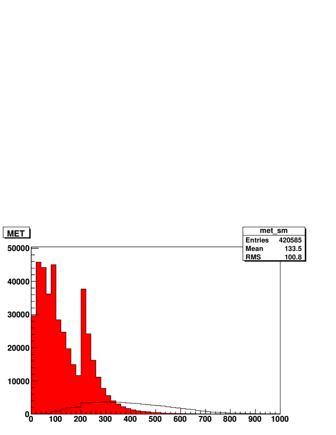
The choice of cut can be motivated by the plot in figure 4, produced for one of the randomly generated spectra. It can be seen that for GeV, the signal dominates over the background. This value does not depend significantly on the choice of the random spectrum.
The simplest signatures to consider are inclusive counts of opposite sign di-lepton and tri-lepton events (including taus). These are also among the most promising for SUSY searches since the detector tagging efficiency for leptons (electrons and muons in particular) is quite high. Furthermore, there is relatively little Standard Model background for multi-lepton multi-jet high- events.
The presence of many opposite sign di-leptons is also an indicator of whether the decay chain occurs frequently in the samples. This decay chain may be used [62] for constructing an endpoint which can subsequently be used to constrain sparticle masses. The results for spectra with fixed at GeV are shown in Figure 5.
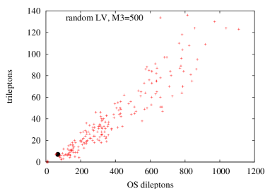
Even though the overall mass scale of the spectrum is fixed and the SUSY cross-section is essentially unaltered between models, there is still a large range for the number of observed di-lepton and tri-lepton events. The dominant background comes from events, and in a large number of cases the number of such SUSY events lies above the acceptable number of background events.
This variation can be understood in terms of the different possible spectra, The number of di-lepton (and hence tri-lepton) events depends crucially on the details of the decay chain. In most cases the first 2 generations of left handed sleptons are heavier than . However the right handed sleptons may be lighter or heavier than . If they are all heavier, then the 3-body decays of the will dominate. The decay will then often proceed through an off-shell slepton , giving many di-lepton events. However, if are heavier than but is lighter - which can occur as, for larger , is driven down by the RGEs and tends to be light - the will predominantly decay through the chain . Since the tau tagging efficiency is relatively low, and is relatively small (meaning that the taus tend to be soft), few taus will be picked up by the detector. It may also happen that all of are lighter than , with the dominant branching ratio of again into s and s. In this case we again observe only a few di-lepton or tri-lepton events.
In ref. [61], the number of clean di- and tri- leptons was used as an observable, meaning no jet activity in the detector. From the point of view of our simulation, this corresponds to direct weak gaugino and/or slepton production. In 10 fb-1, none of our model samples produced a single “clean” event, consistent with the masses of the sleptons/weak gauginos and the fact that this is a weakly interacting production channel. The usefulness of this observable is questionable, since there will always be some jet pollution in the detectors due to the QCD background. Thus some cut on hadronic activity must be given experimentally in order to define a jet veto, and the predicted backgrounds can be notoriously unreliable.
Another observable considered in [61] that we will not use here concerns the number of events with no leptons, 1 or 2 -jets, and at least six hard jets. The difficulty in using this observable comes in the estimation of the background. The processes in PYTHIA are rather than , and so the ‘hard jet’ background arising from PYTHIA comes from the parton shower rather than from direct hard jet production. This may underestimate the background by orders of magnitude. A correct estimate of this background would require the inclusion of processes in the Monte Carlo (e.g. with ALPGEN [63]).

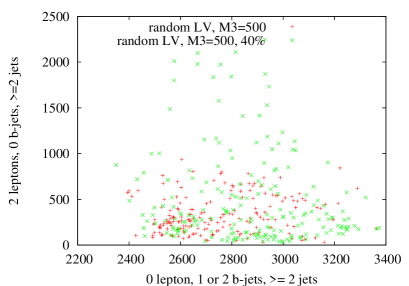
In figure 6, we plot the number of di-lepton multi-jet events with 1 or 2 -jets against the number of di-lepton multi-jet events with 0 -jets. There is a clear positive correlation in Fig. 6, indicating that the number of events with two leptons and -jets is dependent more on the number of events with leptons passing the cuts than on the number of -jets. Nonetheless the number of events with -jets can vary by a factor of 2 between different spectra. This is reasonable, because there are numerous competing decays where the branching ratios are dependent on various independent input parameters. We give one example. If kinematically allowed, as here, the gluino has a significant branching ratio to , which generates events with multi-jets and s. The branching ratios of and depend on and , since they affect the mixing of the stops. In figure 6 we also require two leptons. However the number of leptons observed depends on the mass differences between the light neutralinos and the sleptons. The point is that these parameters mentioned above are varied independently in our models, which explains why spectra with similar numbers of leptons can have different numbers of -jets. Other decay chains, for example , can be analysed in a similar fashion.
The number of -jets may potentially be used as a coarse discriminator between different high-scale constructions. Suppose the scalars are much heavier than the gluino, with a large Higgsino component to the LSP. In this situation, the gluino will primarily decay through a 3 body channel to - as well as other channels involving tops if kinematically allowed - due to the large higgsino coupling to stops and sbottoms. These decays will all result in a large number of -jet events. An example of such a construction is the focus point region of mSUGRA. Since in our construction the light neutralinos are always gaugino dominated, the number of -jet events is expected to be smaller. We have verified that a focus point spectrum does indeed give many more -jet events than those arising from the large-volume models. Thus, once -jet tagging is understood, the number of -jets can potentially be used to distinguish different high-scale constructions with a similar overall production scale.
Since the random variation we chose for all parameters is an arbitrary choice, it is useful to compare the results with a sample of spectra with variations. The results (again with GeV at the high scale) are shown in figures 7-8. In figure 7 we see the number of di- and tri-lepton events, as well as the number of di-lepton events with or without -jets. The general structure of the observables is similar to that seen above with the variations. However the variation spectra, although with the same overall mass scale (as defined by the gluino mass) can have significantly more di-lepton events than the variation spectra. This is due to the fact that in the case, the LSP is more likely to acquire a significant wino component, in which case the large left-handed couplings result in a lot of lepton production Also it may happen that all the right handed sleptons and left handed sleptons are lighter than , and that the mass differences are all large, which again results in many observed di-lepton events.
An interesting counting observable to consider is the number of events with one or two -jets, requiring 2 hard jets in the event. In figure 8 we compare the number of di-lepton events without -jets against the number of 0 lepton events with -jets. This observable is shown on the abscissa of figure 8, and it is consistent throughout the entire sample of spectra. The observability limit defined by Eq. (59) is at (209,49) and is omitted from the figure.
4.2.1 Varying the Sparticle Mass Scale
We next investigate the effect of varying the overall mass scale which has so far been set by fixing the gluino mass. An arbitrary value for is selected and variations on the parameter allowed. The results are shown in figures 9-10, in conjunction with the results for the SPS1a slope given by . In the plots, 50 SPS1a points from GeV to GeV in steps of 13 GeV are shown.
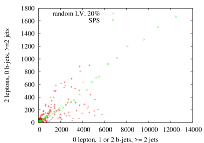
The main conclusion from the study of counting observables is that, even with the spectra restricted to the form of figures 2 and 3, the total number of observed SUSY events can vary widely. Even fixing the overall scale of the spectrum, the large-volume models still lead to a widely varying number of triggered events: models at the same scale and coming from the same high-scale theory can give quite different results as small changes in high scale parameters can lead to significant changes in observables. We do not make an explicit comparison of our results with the models discussed in [61] for this reason. If there is so much variation within our models, there will be a larger variation with other models that would make them difficult to differentiate. We have also used different cuts, which makes a quantitative comparison impossible. Nonetheless, a rough look at the similar plots in both works does not indicate an easy way to separate these models from those in [61].
4.3 Potential for Reconstruction
We now discuss the potential for reconstructing the spectra of figure 2. This will illustrate the above point: if there are very few di-lepton events, and no kinematic endpoints, then direct reconstruction would be very difficult if not impossible. The structure of the analysis given here follows standard accounts of reconstruction such as in ref. [62, 64], for example.
The ability to reconstruct supersymmetric particle masses depends significantly on the spectrum and on the decay chains and their branching ratios. Since jet observables usually suffer from large combinatorial backgrounds, the cleanest measurements are those involving only leptons. Therefore the first step in reconstruction of a supersymmetric spectrum is a measurement of a di-lepton edge from the chain. As explained in section 4.2, whether we observe few or many di-lepton events from this decay chain is determined by the mass difference between and and the slepton branching ratios. Figure 11 shows the plot of the di-lepton invariant mass for 10 of data for two spectra, one with many opposite sign, same flavour (OSSF) di-lepton events in the signal, and one with very few. There is no evidence for an edge in the di-lepton invariant mass in Fig. 11b. If there are few di-lepton events, the spectrum is much harder to reconstruct since one has to resort to multi-jet observables.
We therefore restrict to considering a spectrum which generates many OSSF di-lepton events, such that the di-lepton edge can be easily reconstructed. For this spectrum we simulated data and the plots given are based on this simulation. This represents one year of LHC running at design luminosity. The spectrum we attempt to reconstruct is as shown in Table 1.
| 303 | 480 | 114 | 532 | 532 | 538 | ||||
| 909 | 800 | 792 | 779 | 583 | 790 | 725 | 782 | 787 | |
| 348 | 261 | 338 | 336 | 270 | 349 | 233 | 303 | 460 | 483 |
We start by selecting events that pass a set of cuts that we name selection A:
-
1.
-
2.
Two opposite sign electrons or muons with GeV.
-
3.
At least four jets with .
-
4.
, where .
We then plot the histogram of the di-lepton invariant mass, with a flavour subtraction of the result to cancel processes with leptons arising from two independent decays.
This plot is shown in figure 12.
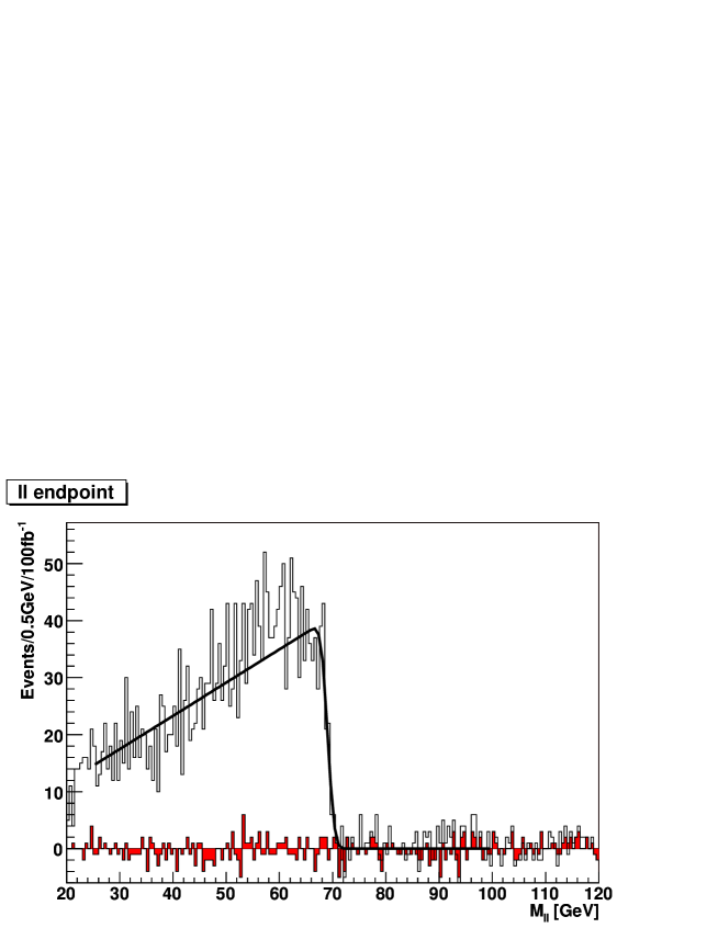
It is well-known [62] that the decay chain admits an endpoint at
| (60) |
The location of this endpoint can be found by fitting figure 12 with a triangular edge, smeared with a Gaussian (the width of which is also fitted) to simulate resolution effects of the experiment. MINUIT [66] and MINOS are used for this purpose, and to estimate the error on the measurement. We obtain GeV.
Following Ref. [62], we next study the decay channel to obtain a set of constraints on the squark masses as well as , Events are selected with the following properties (selection B):
-
1.
At least 4 hard jets, with .
-
2.
Two opposite sign electrons or muons with GeV.
-
3.
.
-
4.
The di-lepton 4-momentum is combined with each of the two hardest jets to obtain two different invariant masses. The lighter of these is plotted in figure 13.
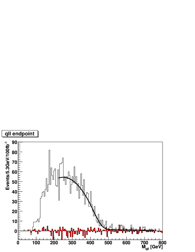
can be written in terms of the maximum of several terms that contain sparticle masses and have a form similar to Eq. 60. In refs. [64, 62], rather simple expressions were given for edges such as . These were correct for the particular mass spectra examined in those papers, but are not true in the general case. We therefore use the general expressions given in Ref. [65] and refer the reader there for further details. An empirical fit of the form
| (61) |
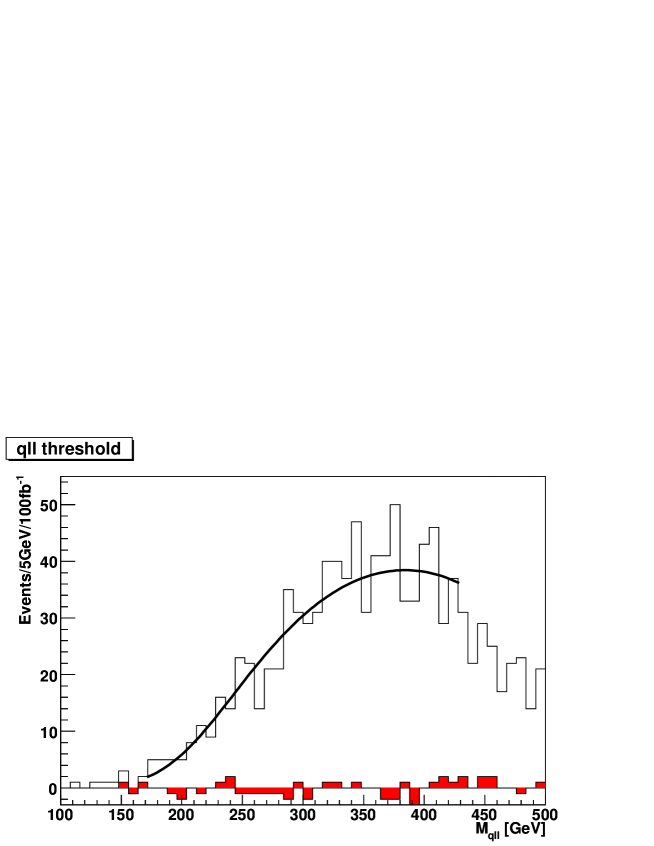
is used to reconstruct this endpoint with GeV. With a variable in the fit, MINOS did often not converge, indicating a possible degenerate minimum valley. With a fixed width, we were able to obtain a perfectly good fit, as Fig. 13 shows. The endpoint obtained through this fit is GeV. Where we quote two uncertainties, the first is a statistical one from the fitting procedure whereas the second is our guess at an additional ‘fitting’ systematic uncertainty from seeing the effect of changing the bin-size and fit interval. For events in which , the larger mass is plotted in figure 14.141414The flavour subtraction of the Standard Model background in figures 13 and 15 and can be seen to slightly over subtract. This can be understood as an artifact of the triggers used, which have a small flavour asymmetry.
This gives a threshold which has a theoretical locus in terms of masses of all four sparticles involved in the chain [65]. The threshold is obtained by fitting with the empirical form
| (62) |
and a Gaussian smearing. We obtain GeV from the fit, which Fig. 14 shows, reproducing the shape of binned simulated data up to statistical variations.
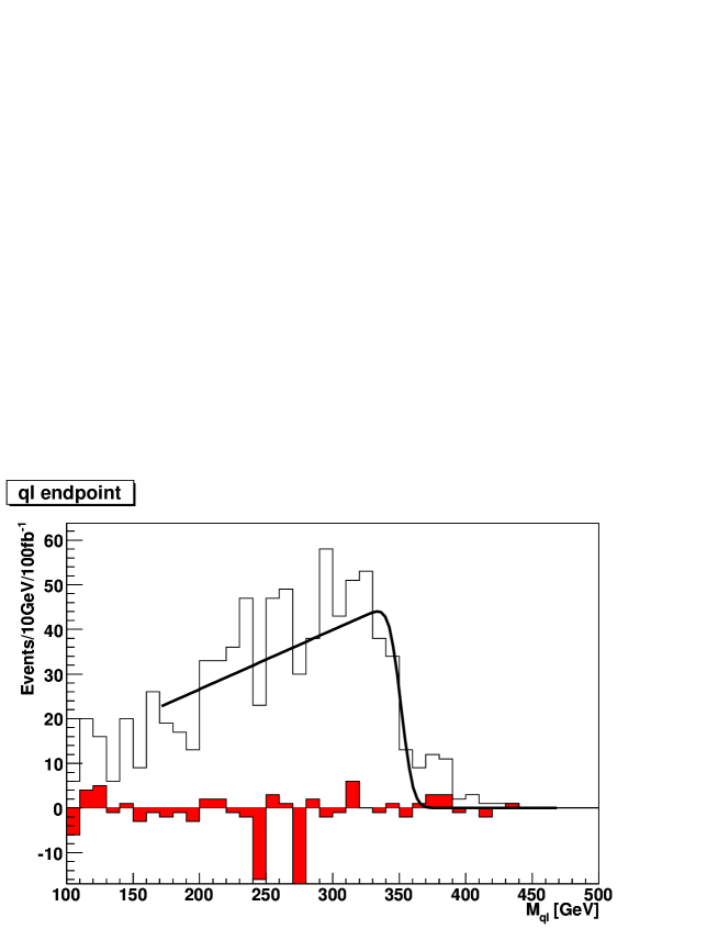
Events are then further selected such that one mass is less than and the other greater than GeV. This identifies the jet involved in the decay chain . By combining each of the leptons with this jet, we can plot the mass (figure 15) which constrains a function of the sparticle masses [65]. This endpoint is located in a similar fashion to the di-lepton endpoint, using a Gaussian smeared triangular fit. We obtained GeV.
We summarise the values found through the above fitting procedure in Table 2. They differ from the expected values by ‘experimental’ systematic errors. The sources for these systematic errors can be associated with hadronic calorimeter calibration, jet energy leakage or the cone or cluster algorithms that reconstruct the jets. For our purposes we assume that these systematic errors can be removed as part of the experimental analysis. Following [64], for our estimation of sparticle masses we shift the measured endpoints to the theoretical values, thus eliminating this experimental systematic bias, but keep the errors arising from the fitting procedure. We add the statistical and ‘fitting’ systematic errors in quadrature in order to quote a total uncertainty on the central theoretical value.
| Fitted value/GeV | Shifted value/GeV | |
|---|---|---|
| 69.4 0.15 | 69.40.15 | |
| 4505.52.4 | 467.66.0 | |
| 3531.73.6 | 370.84.0 | |
| 1887.56.6 | 202.810.0 |
We now use these shifted endpoints to reconstruct the and masses. To do so, we take and to be randomly generated with a uniform distribution within 50% of their central values and compute using the di-lepton endpoint which has a very small statistical error. This is equivalent to approximating the very narrow Gaussian likelihood distribution of with a function. We then compute the for the remaining observables () and assign a weight to this set of randomly generated masses. Doing this many times provides a sampling of a probability distribution for the sparticle masses. The marginalisations to three independent mass differences is shown in figure 16.
| Theoretical/GeV | Estimated/GeV | |
|---|---|---|
| 37.5 | 28.11.4, 37.52.3 | |
| 69.7 | 69.7 | |
| 567 | 56426 |
From each probability distribution, we estimate the mass differences. The histograms show the binned estimated probability density function of each mass difference, whereas the continuous lines show the best-fit Gaussian shape. In Fig. 16a, the plot has been separated into two regions, each of which is fitted with a separate Gaussian. has been fitted with two half-Gaussians of different widths, “glued” at the maximum. is not very well fitted with a Gaussian, as Fig. 16c shows. We characterise the distribution instead by its mean and standard deviation. The characteristic double-bump structure of Fig. 16a displays the existence of two solutions in mass space for the edge variables listed in Table 2 and results in two different possible estimated values for the mass difference, one at each local maximum. This ambiguity was also observed for the case of an LHC SPS1a spectrum reconstruction in [67]. We display the estimated and theoretical values for the three mass differences in Table 3. In our case, the ’true’ peak correspond to the ql-edge given by invariant mass of the quark and the far lepton in the decay chain, whereas the ’wrong’ peak correspond to a solution for the ql-edge given by the quark and the near lepton. We find the ‘wrong’ solution by numerical scans to be GeV, GeV, GeV and GeV with a resulting of 0 (the solution of the correct peak also has a zero value of , by construction). The different heights of the bumps in Fig. 16 must therefore be a consequence of volume effects in the marginalisation procedure, since the two best-fit solutions are equally likely. One requires additional data in order to discriminate between the two solutions experimentally.
Despite the existence of two possible good-fit regions of mass difference space, we have enough information to discriminate against mSUGRA models. As mentioned before, the gaugino mass ratios in mSUGRA are We also know that in mSUGRA, is strongly correlated with and generically we have (this is guaranteed within mSUGRA by the presence of light sleptons). Therefore, in mSUGRA models we have and
However, for the large volume models we obtain
| (63) |
from Table 3. Thus the measurements made are not compatible with the mSUGRA scenario. Further measurements, e.g. of the gluino mass and the right handed squark masses, would provide further evidence for discrimination against mSUGRA. Using the expected ratios, we could also investigate the prediction of the large volume models. For this it would be useful to directly measure the gluino mass: to this end the decay channel may be exploited as well as the variable [68].
5 Conclusions
We have performed a detailed study of the expected superparticle spectrum and collider phenomenology for large-volume string models. Our main conclusions are:
-
1.
The large volume models give rise to a distinctive spectrum of gaugino masses, characterised by
(64) This can be distinguished from the ratios that appear in e.g. mirage mediation or mSUGRA.
The collider phenomenology depends heavily on the mass difference between and and the slepton mass spectrum. If this is large, leading to many events, kinematical reconstruction of the spectrum is much easier. This was discussed in section 4.
-
2.
The overall spectrum tends to be more bunched than that of a corresponding mSUGRA model. This can be understood by the approximate unification, prior to the inclusion of the effects of magnetic fluxes on the brane world-volume, of scalar and gaugino masses at the intermediate (fundamental) scale. There is then less energy for the physical masses to evolve from their theoretical boundary condition and the overall spectrum falls within a narrower mass range.
This effect also occurs in models of mirage mediation, where gaugino masses are (accidentally) unified at the intermediate scale.
-
3.
More concretely we find: the LSP is mostly bino. The second neutralino is mostly wino and is almost degenerate with charginos. Sleptons are almost degenerate, with stau the lightest. The gluino is the heaviest sparticle. The ratio of the gaugino-squark masses is larger than that predicted by mSUGRA.
-
4.
We have quantified the uncertainty that appears in the weak scale spectra due to uncertainties in the high-energy soft terms. The incorporation of such uncertainties is essential in trying to make predictions for LHC signatures based on high-scale string constructions.
-
5.
We have used event generators and detector simulators to study possible signatures of our models. We analysed the use and limitations of certain ‘counting’ observables to contrast our models with other classes of models, especially a line through mSUGRA parameter space (the SPS1a slope) that has been well studied in the literature. We found that some counting observables are more useful than others but in general they do not provide enough information to fully distinguish the models, at least in simple 2-dimensional projections. It may be true that a fit of the models to the full parameter space of counting observables is required.
-
6.
We studied in detail a sample model that is quite rich in decays. Accurate reconstruction of some properties of the low-energy sparticle spectrum is possible with 100 fb-1 of integrated luminosity. Our sample study shows that the large volume model can be differentiated from standard mSUGRA.
In this work we have made progress in the process of starting with a well defined class of microscopic models and bringing them to the point where they may be confronted with potential experimental measurements at the LHC. This is a positive step in the direction of testing classes of models derived from string theory. This is clearly a less ambitious task than testing string theory in its entirety, but one that may prove more fruitful. Moduli stabilisation with supersymmetry breaking has allowed us to find explicit expressions for soft breaking terms that have a well-defined microscopic origin, which is not the case for the well studied standard benchmark points. Issues, such as flavour universality and extra CP violation, that render the generic gravity mediation scenario unrealistic and have to be resolved by hand in most models, can now be understood in terms of the particular properties of string compactifications. Furthermore we have found ways to distinguish our models from mSUGRA and other models, using properties that may be directly measured within a few years of LHC running.
There are however several open questions we need to emphasise. First of all we have been working on a scenario allowed by type II constructions, in which the Standard Model is assumed to live on a set of D-branes localised at a particular region inside the Calabi-Yau manifold. The problems of moduli stabilisation and supersymmetry breaking are thus decoupled from the details of the Standard Model construction. This approach has the positive feature that moduli are stabilised in a large class of models. Other issues, such as the number of families, proton stability and gauge unification are more model dependent. In this sense our results are very robust. On the other hand they lack concreteness in the sense that we do not have an explicit D-brane configuration with the MSSM spectrum, known Yukawa couplings, etc. Finding a fully realistic model in this approach is therefore an open question.
Nevertheless we have identified the main sources of uncertainty in our analysis that parametrise our ignorance of such a realistic model. First, we included the effects of magnetic fluxes, usually needed to construct chiral models on D7 branes. Even though the dependence of Kähler potentials and gauge couplings on the magnetic fluxes is not known, we were able to parametrise our ignorance in terms of the random parameters . A second source of uncertainty is the spectrum itself. We know that typical quasi-realistic D-brane models (see [69] for a recent review) usually have extra particles beyond the MSSM and that the hypercharge does not have a canonical normalisation. We took into account these effects by varying the hypercharge normalisation and finding observables, such as the ratios of gaugino masses, which do not change if there are extra fields beyond the MSSM. Finally, we have assumed the simplest configuration of D7 branes hosting the Standard Model in the sense that they are all assumed to wrap the same 4-cycle. Different configurations would slightly change the expressions for the soft breaking terms. The expressions would then depend on an extra parameter that takes different values depending upon which cycles the branes wrap and the manner of their intersection. For the case studied here, [13, 12]. It would be interesting to explore the implications of other configurations leading to different values of .
The model independence of our analysis makes it easy to adapt once explicit realistic models are constructed that may differ from the MSSM. Furthermore, potential experimental measurements at the LHC may provide guidance on what the structure of these realistic models should be. Even if at the end it turns out that our models will not pass experimental scrutiny from the LHC, the detailed analysis made, all the way from string theory to LHC observables, should be a useful guide for future proposals. It is encouraging to have this rich interplay between theory and experiment waiting for the arrival of LHC results.
Acknowledgements
This work has been partially supported by STFC.151515Formerly PPARC (R.I.P.) We thank Shehu Abdussalam, Marcus Berg, Kiwoon Choi, Daniel Cremades and the members of the Cambridge SUSY working group for useful conversations. We particularly thank our colleagues that wrote and made available the many codes we have used in this work. The computational work has been performed using the Cambridge eScience CAMGRID computing facility, with the invaluable help of Mark Calleja and Andy Parker. JC and KS are funded by Trinity College, Cambridge. BCA is funded by STFC. FQ is partially funded by STFC and a Royal Society Wolfson award. CHK is supported by a Dorothy Hodgkin Postgraduate Award.
Appendix A PGS Level 2 Triggers
Here we list the PGS Level 2 Triggers used in our event analysis for ease of reference, which can be obtained from pgs_olympics.f in the PGS package [9]. If any of the following apply to an event, the trigger is passed and the event recorded. The PGS definition of isolation is somewhat involved, and we refer the interested reader to the PGS manual for further details. Our isolation criteria for muons are based on those used in the Chameleon [70] package: the ratio of the energy in a 3x3 grid surrounding the muon and the of the muon is required to be 0.1125, and the total of a cone region surrounding (but excluding) the muon is required to be GeV.
-
1.
Inclusive isolated lepton GeV;
-
2.
For a lepton GeV plus a jet GeV;
-
3.
Isolated same-flavour di-leptons GeV;
-
4.
Di-leptons GeV plus jet GeV;
-
5.
Isolated opposite-flavour di-leptons GeV;
-
6.
Isolated lepton GeV plus isolated tau GeV;
-
7.
Isolated di-tau GeV;
-
8.
Inclusive isolated photon GeV;
-
9.
Isolated di-photon GeV;
-
10.
Inclusive GeV;
-
11.
Inclusive single-jet GeV;
-
12.
Jet GeV plus GeV;
-
13.
Acoplanar jet GeV and GeV, ;
-
14.
Acoplanar dijets GeV, .
References
- [1] V. Balasubramanian, P. Berglund, J. P. Conlon and F. Quevedo, “Systematics of moduli stabilisation in Calabi-Yau flux compactifications,” JHEP 0503, 007 (2005) [arXiv:hep-th/0502058].
- [2] J. P. Conlon, F. Quevedo and K. Suruliz, “Large-volume flux compactifications: Moduli spectrum and D3/D7 soft supersymmetry breaking,” JHEP 0508, 007 (2005) [arXiv:hep-th/0505076].
- [3] S. Kachru, R. Kallosh, A. Linde and S. P. Trivedi, “De Sitter vacua in string theory,” Phys. Rev. D 68, 046005 (2003) [arXiv:hep-th/0301240].
- [4] K. Becker, M. Becker, M. Haack and J. Louis, “Supersymmetry breaking and alpha’-corrections to flux induced potentials,” JHEP 0206, 060 (2002) [arXiv:hep-th/0204254].
- [5] V.Balasubramanian and P.Berglund “Stringy corrections to Kahler potentials, SUSY breaking, and the cosmological constant problem,” JHEP 0411, 085 (2004) [arXiv:hep-th/0408054].
- [6] B. S. Acharya, K. Bobkov, G. L. Kane, P. Kumar and J. Shao, “Explaining the electroweak scale and stabilizing moduli in M theory,” [arXiv:hep-th/0701034].
- [7] G. Corcella et al., “HERWIG 6: An event generator for hadron emission reactions with interfering gluons (including supersymmetric processes),” JHEP 0101 (2001) 010 [arXiv:hep-ph/0011363].
- [8] T. Sjostrand, S. Mrenna and P. Skands, “PYTHIA 6.4 physics and manual,” JHEP 0605 (2006) 026 [arXiv:hep-ph/0603175].
- [9] http://www.physics.ucdavis.edu/ conway/research/software/pgs/pgs4-general.htm
- [10] B. C. Allanach, F. Quevedo and K. Suruliz, “Low-energy supersymmetry breaking from string flux compactifications: Benchmark scenarios,” JHEP 0604 (2006) 040 [arXiv:hep-ph/0512081].
- [11] J. P. Conlon and F. Quevedo, “Gaugino and scalar masses in the landscape,” JHEP 0606 (2006) 029 [arXiv:hep-th/0605141].
- [12] J. P. Conlon, S. S. Abdussalam, F. Quevedo and K. Suruliz, “Soft SUSY breaking terms for chiral matter in IIB string compactifications,” JHEP 0701 (2007) 032 [arXiv:hep-th/0610129].
- [13] J. P. Conlon, D. Cremades and F. Quevedo, “Kaehler potentials of chiral matter fields for Calabi-Yau string compactifications,” JHEP 0701 (2007) 022 [arXiv:hep-th/0609180].
- [14] G. von Gersdorff and A. Hebecker, “Kaehler corrections for the volume modulus of flux compactifications,” Phys. Lett. B624 270-274 (2005) [arXiv:hep-th/0507131].
- [15] M. Berg, M. Haack and B. Kors, “String loop correctios to Kahler potentials in orientifolds,” JHEP 0511 (2005) 030 [arXiv:hep-th/0508043].
- [16] M. Berg, M. Haack and E. Pajer, “Jumping Through Loops: On Soft Terms from Large Volume Compactifications,” [arXiv:0704.0737] [hep-th].
- [17] J. P. Conlon and F. Quevedo, “Kaehler moduli inflation,” JHEP 0601 (2006) 146 [arXiv:hep-th/0509012]; R. Holman and J. A. Hutasoit, “Systematics of moduli stabilization, inflationary dynamics and power JHEP 0608 (2006) 053 [arXiv:hep-th/0606089]; J. R. Bond, L. Kofman, S. Prokushkin and P. M. Vaudrevange, “Roulette inflation with Kaehler moduli and their axions,” [arXiv:hep-th/0612197].
- [18] J. P. Conlon, “The QCD axion and moduli stabilisation,” JHEP 0605, 078 (2006) [arXiv:hep-th/0602233].
- [19] J. P. Conlon and D. Cremades, “The neutrino suppression scale from large volumes,” [arXiv:hep-ph/0611144].
- [20] J. P. Conlon, “Moduli stabilisation and applications in IIB string theory,” arXiv:hep-th/0611039.
- [21] S. Gukov, C. Vafa and E. Witten, “CFT’s from Calabi-Yau four-folds,” Nucl. Phys. B 584, 69 (2000) [Erratum-ibid. B 608, 477 (2001)] [arXiv:hep-th/9906070].
- [22] T. W. Grimm and J. Louis, “The effective action of N = 1 Calabi-Yau orientifolds,” Nucl. Phys. B 699, 387 (2004) [arXiv:hep-th/0403067].
- [23] F. Denef, M. R. Douglas and B. Florea, “Building a better racetrack,” JHEP 0406, 034 (2004) [arXiv:hep-th/0404257].
- [24] C. P. Burgess, R. Kallosh and F. Quevedo, “de Sitter string vacua from supersymmetric D-terms,” JHEP 0310 (2003) 056 [arXiv:hep-th/0309187]; A. Saltman and E. Silverstein, “The scaling of the no-scale potential and de Sitter model building,” JHEP 0411 (2004) 066 [arXiv:hep-th/0402135].
- [25] D. Cremades, M. P. Garcia del Moral, F. Quevedo and K. Suruliz, “Moduli stabilisation and de Sitter string vacua from magnetised D7 branes,” [arXiv:hep-th/0701154].
- [26] G. Aldazabal, L. E. Ibanez, F. Quevedo and A. M. Uranga, “D-branes at singularities: A bottom-up approach to the string embedding of the standard model,” JHEP 0008, 002 (2000) [arXiv:hep-th/0005067]; J. F. G. Cascales, M. P. Garcia del Moral, F. Quevedo and A. M. Uranga, “Realistic D-brane models on warped throats: Fluxes, hierarchies and moduli stabilization,” JHEP 0402 (2004) 031 [arXiv:hep-th/0312051].
- [27] M. Buican, D. Malyshev, D. R. Morrison, M. Wijnholt and H. Verlinde, “D-branes at singularities, compactification, and hypercharge,” JHEP 0701, 107 (2007) [arXiv:hep-th/0610007].
- [28] M. Wijnholt, “Geometry of particle physics,” [arXiv:hep-th/0703047].
- [29] D. Lust, P. Mayr, R. Richter and S. Stieberger, “Scattering of gauge, matter, and moduli fields from intersecting branes,” Nucl. Phys. B 696, 205 (2004) [arXiv:hep-th/0404134].
- [30] D. Lust, S. Reffert and S. Stieberger, “Flux-induced soft supersymmetry breaking in chiral type IIb orientifolds with D3/D7-branes,” Nucl. Phys. B 706, 3 (2005) [arXiv:hep-th/0406092].
- [31] A. Brignole, L. E. Ibanez and C. Munoz, “Soft supersymmetry-breaking terms from supergravity and superstring models,” [arXiv:hep-ph/9707209].
- [32] G. F. Giudice and A. Masiero, “A Natural Solution to the mu Problem in Supergravity Theories,” Phys. Lett. B 206 (1988) 480.
- [33] R. Blumenhagen, B. Kors, D. Lust and S. Stieberger, “Four-dimensional string compactifications with D-branes, orientifolds and fluxes,” [arXiv:hep-th/0610327].
- [34] B. C. Allanach, “SOFTSUSY: A C++ program for calculating supersymmetric spectra,” Comput. Phys. Commun. 143, 305 (2002) [arXiv:hep-ph/0104145].
- [35] [Tevatron Electroweak Working Group], “Combination of CDF and D0 results on the mass of the top quark,” [arXiv:hep-ex/0608032].
- [36] W. M. Yao et al. [Particle Data Group], “Review of particle physics,” J. Phys. G 33, 1 (2006).
-
[37]
Heavy Flavour Averaging Group Collaboration.
http://www.slac.stanford.edu/xorg/hfag - [38] P. Gambino, U. Haisch and M. Misiak, “Determining the sign of the b s gamma amplitude,” Phys. Rev. Lett. 94, 061803 (2005) [arXiv:hep-ph/0410155].
- [39] G. W. Bennett et al. [Muon g-2 Collaboration], “Measurement of the negative muon anomalous magnetic moment to 0.7-ppm,” Phys. Rev. Lett. 92, 161802 (2004) [arXiv:hep-ex/0401008].
- [40] F. Jegerlehner, “Essentials of the Muon g-2,” [arXiv:hep-ph/0703125].
- [41] J. P. Miller, E. de Rafael and B. L. Roberts, “Muon g-2: Review of theory and experiment,” [arXiv:hep-ph/0703049].
- [42] R. Barate et al. [ALEPH Collaboration], “Search for the standard model Higgs boson at LEP,” Phys. Lett. B 565, 61 (2003) [arXiv:hep-ex/0306033].
- [43] D. N. Spergel et al., “Wilkinson Microwave Anisotropy Probe (WMAP) three year results: Implications for cosmology,” [arXiv:astro-ph/0603449].
- [44] G. Belanger, F. Boudjema, A. Pukhov and A. Semenov, “MicrOMEGAs: Version 1.3,” Comput. Phys. Commun. 174, 577-604 (2006) [arXiv:hep-ph/0405253].
- [45] J. Conlon, F. Quevedo, “Astrophysical and Cosmological Implications of Large Volume String Compactifications,” [arXiv:hep-ph/0705.3460].
- [46] D. R. Tovey, “Measuring the SUSY mass scale at the LHC]], Phys. Lett. B 498 (2001) 1 [arXiv:hep-ph/0006276].
- [47] S. P. Martin, “A supersymmetry primer,” [arXiv:hep-ph/9709356].
- [48] K. Choi and H. P. Nilles, “The gaugino code,” [arXiv:hep-ph/0702146].
- [49] S. A. Abel and B. Allanach, “The quasi-fixed minimal supersymmetric standard model,” Phys. Lett. B 415 (1997) 371 [arXiv:hep-ph/9707436].
- [50] K. Choi, A. Falkowski, H. P. Nilles and M. Olechowski, ’‘Soft supersymmetry breaking in KKLT flux compactification,” Nucl. Phys. B 718, 113 (2005) [arXiv:hep-th/0503216];
- [51] M. Endo, M. Yamaguchi and K. Yoshioka, “A bottom-up approach to moduli dynamics in heavy gravitino scenario: Superpotential, soft terms and sparticle mass spectrum,” Phys. Rev. D 72, 015004 (2005) [arXiv:hep-ph/0504036].
- [52] K. Choi, K. S. Jeong and K. i. Okumura, “Phenomenology of mixed modulus-anomaly mediation in fluxed string compactifications and brane models,” JHEP 0509, 039 (2005) [arXiv:hep-ph/0504037].
- [53] K. Choi, K. S. Jeong, T. Kobayashi and K. Okumura “TeV scale mirage mediation and natural SUSY hierachy,” [arXiv:hep-ph/0612258].
- [54] W. S. Cho, Y. G. Kim, K. Y. Lee, C. B. Park and Y. Shimizu, “LHC signature of mirage mediation,” [arXiv:hep-ph/0703163].
- [55] H. Baer, E. K. Park, X. Tata and T. T. Wang, “Collider and dark matter phenomenology of models with mirage unification,” [arXiv:hep-ph/0703024].
- [56] A. Falkowski, O. Lebedev, Y. Mambrini, “SUSY phenomenology of KKLT flux compactifications,” JHEP 0511, 034 (2005) [arXiv:hep-ph/0507110].
- [57] P. Skands et al., “SUSY Les Houches accord: Interfacing SUSY spectrum calculators, decay packages, and event generators,” JHEP 0407, 036 (2004) [arXiv:hep-ph/0311123].
- [58] http://physics.princeton.edu/ verlinde/research/lhco/ http://ph-dep-th.web.cern.ch/ph-dep/th/lhcOlympics/lhcolympicsII.html. http://www.phys.washington.edu/users/strasslr/LHCO.BBpage.html.
- [59] R. Brun and F. Rademakers, “ROOT- An Object Oriented Data Analysis Framework ” Nucl. Inst. & Meht. in Phys. Res. A 389 (1997) 81-86.
- [60] W. Beenakker, R. Hopker, M. Spria and P. M. Zerwas, “Squark and Bluino Production at Hadron Colliders,” Nucl. Phys. B 492 51-103 (1997) [arXiv:hep-ph/9610490].
- [61] G. L. Kane, P. Kumar and J. Shao, “LHC string phenomenology,” [arXiv:hep-ph/0610038].
- [62] ATLAS Collaboration, Technical Design Report, CERN/LHCC/99-15 (1999)
- [63] M. L. Mangano, M. Moretti, F. Piccinini, R. Pittau and A. Polosa, “ALPGEN, a generator for hard multiparton processes in hadronic collisions” JHEP 0307, 001 (2003) [arXiv:hep-ph/0206293].
- [64] H. Bachacou, I. Hinchliffe and F. E. Paige, “Measurements of Masses in SUGRA Models at LHC” Phys. Rev. D 62, 015009 (2000) [arXiv:hep-ph/9907518]
- [65] B. C. Allanach, C. G. Lester, M. A. Parker and B. R. Webber, “Measuring sparticle masses in non-universal string inspired models at the LHC”, JHEP 0009 (2000) 004 [arXiv:hep-ph/0007009].
- [66] http://wwwasdoc.web.cern.ch/wwwasdoc/WWW/minuit/minmain/minmain.html.
- [67] B. K. Gjelsten, D. J. Miller and P. Osland, “Measurement of SUSY masses via cascade decays for SPS 1a,” JHEP 0412, 003 (2004) [arXiv:hep-ph/0410303]; B. K. Gjelsten, D. J. Miller and P. Osland, “Measurement of the gluino mass via cascade decays for SPS 1a,” JHEP 0506, 015 (2005) [arXiv:hep-ph/0501033]. C. G. Lester, M. A. Parker and M. J. White, “Determining SUSY model parameters and masses at the LHC using cross-sections, kinematic edges and other observables,” JHEP 0601 (2006) 080 [arXiv:hep-ph/0508143].
- [68] C. G. Lester and D. J. Summers, “Measuring masses of semi-invisibly decaying particles pair produced at hadron colliders,” Phys. Lett. B 463, 99-103 (1999) [arXiv:hep-ph/9906349] A. Barr, C. Lester and P. Stephens, “m(T2): The Truth behind the glamour,” J. Phys. G 29, 2343-2363 (2003) [arXiv:hep-ph/0304226]
- [69] F. Marchesano, “Progress in D-brane model building,” [arXiv:hep-th/0702094].
- [70] http://www.jthaler.net/olympics/software.html