Quantized spin excitations in a ferromagnetic microstrip from microwave photovoltage measurements

Abstract

Quantized spin excitations in a single ferromagnetic microstrip have been measured using the microwave photovoltage technique. Several kinds of spin wave modes due to different contributions of the dipole-dipole and the exchange interactions are observed. Among them are a series of distinct dipole-exchange spin wave modes, which allow us to determine precisely the subtle spin boundary condition. A comprehensive picture for quantized spin excitations in a ferromagnet with finite size is thereby established. The dispersions of the quantized spin wave modes have two different branches separated by the saturation magnetization.

Understanding quantized spin excitations in ferromagnets with finite size is not only pivotal for exploring nanomagnetism Tulapurkar2004 , but also essential for designing high-density magnetic memories with fast recording speed Prinz1998 . The most compelling topics that have recently attracted great interest include: the interplay between dipole-dipole and exchange interactions Jorzick1999 ; Jorzick2002 ; Wang2002 ; Park2002 , the characteristics of the spin boundary conditions Rappoport2004 , and the evolution of spin excitations in various phases Wang2002 ; Tartakovskaya2005 ; Wang2005 . Despite general consensus on the theoretical explanation of the combined effects of dipole-dipole and exchange interactions Sparks1970PRB ; Kalinikos1986 , experiments found usually either magnetostatic modes (MSM) White1956 or standing spin waves (SSW) Seavey1958 , which are determined by dipole-dipole or exchange interaction, respectively. As a related problem, the impact of spin boundary conditions, which has been studied over decades on thin films with a thickness comparable to the wavelength of spin waves, remains elusive Rado1959 ; Morrish2001 . The most appealing quantized dipole-exchange spin wave (DESW) modes existing in laterally-structured ferromagnets, which should exhibit combined characteristics of the MSM and SSW, have only been recently observed near the uniform ferromagnetic resonance (FMR) Jorzick1999 ; Jorzick2002 ; Wang2002 ; Park2002 , and are therefore found to be insensitive to the exchange interaction and spin boundary conditions Sparks1970PRB . The lack of a comprehensive picture of spin excitations in ferromagnets with finite size is partially due to the experimental challenge of detecting spin waves in samples with shrinking dimensions, where conventional techniques such as the FMR absorption and Brillouin light scattering are approaching their sensitivity limit.

Very recently, promising new experimental techniques have been developed for studying spin dynamics: microwave photoconductivity Gui2005 and photovoltage techniques Gui2006 , which allow electrical detection of spin excitations in ferromagnetic metals. The associate high sensitivity makes it possible to investigate the comprehensive characteristics of quantized spin excitations.

In this letter we report investigations of quantized spin waves in a single ferromagnetic microstrip using the microwave photovoltage technique. Both the even and odd order SSWs are detected, and quantized DESWs are observed near both the FMR and the SSW. Two distinct branches of the field dispersion for the quantized spin waves are measured. The spin boundary conditions are precisely determined. And an empirical expression describing the dispersion characteristics of the complete spin excitations in the entire magnetic field range is obtained.

Our sample is a Ni₈₀Fe₂₀ (Permalloy, Py) microstrip, with dimensions of $l$ = 2.45 mm, $w$ = 20 $\mu$m, and $d$ = 137 nm as shown in Fig. 1(a) in a $x-y-z$ coordinate system. From anisotropic magnetoresistance measurements, we determine the saturation magnetization $\mu_{0}M_{0}$=1.0 T. As shown in Fig. 1(b), the Py strip is inserted in the slot of a ground-signal-ground coplanar waveguide (CPW) made of an Au/Ag/Cr (5/550/5 nm) multilayer. The device is deposited on a semi-insulating GaAs substrate. By feeding the CPW with a few hundreds mW microwaves, a d.c. voltage $V$ is measured along the $x$-axis as a function of the magnetic field $H$ applied nearly perpendicular to the Py strip. The photovoltage is induced by the spin rectification effect whose characteristics are reported elsewhere Gui2006 . The data presented here are taken by slightly tilting the field direction away from the $z$-axis towards the $x$-axis by a very small angle of 0.2^∘, so that the $x$-component of the magnetization $M_{x}$ is nonvanishing, and the photovoltage $V\propto M_{x}$ has a power sensitivity approaching 0.1 mV/W.

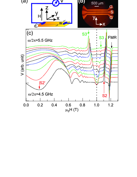
Figure 1: (color online) (a) Schemetic drawing of the Py microstrip and the measurement circuitry. (b) Top view micrograph of a device with Py strips placed in slots between the ground (G) and signal (S) lines of a coplanar waveguide. (c) Typical photovoltage spectra measured at different microwave frequencies (from 4.5 GHz to 5.5 GHz with a step size of 0.1 GHz). Arrows indicate FMR, SSW for the quantized number $p$ = 2 (S2 and S2’) and SSW for $p$ = 3 (S3 and S3’), respectively. The dashed line indicates $H=M_{0}$. All curves are normalized with the FMR amplitude and vertically offset for clarity.

Figure 1(c) shows the electrically-detected quantized spin excitations in the Py microstrip. The sharp resonances at $H>M_{0}$ (labelled as FMR, S2 and S3) move to higher fields with increasing microwave frequency. At high frequencies ($\omega/2\pi>8$ GHz) another resonance (S4) is observed (not shown) at $H>M_{0}$. The dispersions of these resonances follow the well-known Kittel formula for SSWs used in textbooks Morrish2001 , given by: $\omega=\gamma(H-M_{0}+2Ak_{z}^{2}/\mu_{0}M_{0})$. The gyromagnetic ratio is determined to be $\gamma$ = 181 $\mu_{0}$GHz/T. Here $k_{z}=(p-\Delta p)\pi/d$ is the wave vector, and $A$ is the exchange stiffness constant. The quantized number $p$ is the integer number of half wavelengths along the $z$ direction. The correction factor $\Delta p$ is bounded by $0\leq\Delta p\leq 1$ and is determined by the boundary condition Rado1959 :

$$2A\frac{\partial\Psi_{p}}{\partial z}-K_{s}\Psi_{p}=0$$ (1)

where the eigenfunction of SSW has the form $\Psi_{p}=\alpha\sin k_{z}z+\beta\cos k_{z}z$. The constants $\alpha$ and $\beta$ are determined by both the surface anisotropy $K_{s}$ and the exchange stiffness constant $A$. If $\alpha/\beta\rightarrow\infty$, the spins at surfaces are completely pinned and $\Delta p=0$. In the opposite case where $\alpha/\beta\rightarrow 0$, the spins at surfaces are totally free and $\Delta p=1$. Based on the Kittel formula, the observed four resonances correspond to FMR ($p$ = 0) and SSWs with $p$ = 2, 3 and 4. However, the precise values of $\Delta p$, which are dependent on $p$ in general, are difficult to deduce directly from the resonant positions of the SSWs. This is a long standing problem of the spin boundary condition Rado1959 ; Morrish2001 , which not only sets up an obstacle for identifying SSWs, but also causes significant diversity Jorzick2002 ; Park2002 ; Seavey1958 ; Morrish2001 in determining important spin properties such as the value of the exchange stiffness constant $A$.

Before we proceed to determine precisely the value of $\Delta p$ by going beyond the simple Kittel picture, we briefly highlight two interesting features observed in Fig. 1(c). One feature is that there are two branches for each SSW modes. For example, at $\omega/2\pi=4.5$ GHz, the $p$ = 3 SSW mode appears as a dip at $H=M_{0}$. At higher frequencies, it splits into two structures: the higher branch (dips labelled as S3) at $H>M_{0}$ and the lower branch (peaks labelled as S3’) at $H<M_{0}$. Similar effects are observed for other SSWs (see Fig. 3 for the entire dispersions). The higher branch is typical for the SSWs reported earlier, where the magnetization $\mathbf{M}$ is forced to align nearly parallel to $\mathbf{H}$, and the internal field $H_{i}\thickapprox H-M_{0}$. The lower branch is less familiar. Here, $H_{i}\approx$ 0, and the direction of $\mathbf{M}$ is tilted away from the $z$-axis towards the $x$-axis by an angle $\varphi$ given by $cos\varphi\approx H/M_{0}$ Gui2006 . We note that similar evolution of spin waves observed in Ni nanowires Wang2002 and nanorings Wang2005 , were interpreted as reorientation phase transitions Tartakovskaya2005 and the transition from a ”twisted bamboo” state to a ”bamboo” state Wang2005 , respectively.

More interestingly, Fig. 1(c) shows a series of pronounced oscillations between S2’ and S3’. The amplitude of these oscillations decreases with increasing field strength $H$. To the best of our knowledge, such striking oscillations, related to spin dynamics, have never been reported before. They are observed in a series of samples with different thickness in our experiment. As discussed below, the oscillations originate from the lower branch of the DESWs at $H<M_{0}$.

Going beyond Kittel’s picture, the dispersion of DESW modes has a form given by Kalinikos and Slavin Kalinikos1986 :

$$\omega^{2}=\gamma^{2}(H_{i}+2Ak^{2}/\mu_{0}M_{0})(H_{i}+2Ak^{2}/\mu_{0}M_{0}+M_{0}F_{p}),$$ (2)

where

$$F_{p} = P_{p}+\sin^{2}\varphi\left(1-P_{p}+\frac{M_{0}P_{p}(1-P_{p})}{H_{i}+2Ak^{2}/\mu_{0}M_{0}}\right),$$

$$P_{p} = \frac{k_{y}}{2}\int_{0}^{d}\int_{0}^{d}\Psi_{p}(z)\Psi_{p}(z^{\prime})\exp(-k_{y}\mid z-z^{\prime}\mid)dzdz^{\prime}.$$

Here $k^{2}=k_{z}^{2}+k_{y}^{2}$ is the wave vector, and $k_{y}=n\pi/w$ is the quantized wave vector along the $y$ direction. Neglecting the exchange effect ($A$ = 0) the DESW modes near the FMR reduce to the magnetostatic modes with quantized number $n$. In different measurement geometries, magnetostatic modes may appear either as magnetostatic forward volume modes (MSFVM), magnetostatic backward volume modes, or Damon-Eshbach modes Spin2002 . On the other hand, neglecting the dipolar dynamic field by assuming $P_{p}$ = 0, Eq. (2) reduces to the case for SSWs with the quantized number $p-\Delta p$.

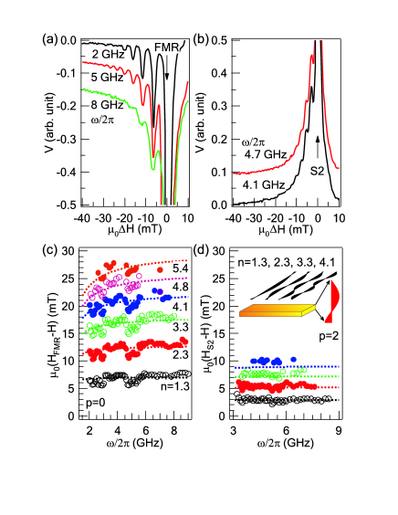
Figure 2: (color online) (a) Quantized MSFVM and (b) DESW modes found near FMR ($p$=0) and SSW ($p$=2), respectively. The spectra are measured at different microwave frequencies and are vertically offset. They are normalized either to FMR or SSW ($p$=2). (c) The measured dispersions (symbols) of the quantized MSFVM and (d) DESW modes are compared with the calculated results (dotted lines). The inset in (d) illustrates the spin waves in the microstrip quantized along both $y$ and $z$ directions.

Both MSFVMs and SSWs are detected by the photovoltage technique in our experiment. If we focus on the low-field range of the FMR, a series of fine structures are well resolved as shown in Fig. 2(a). These are the quantized MSFVMs. The first MSFVM has an intensity of about 25% of that of the FMR and its width is narrower but comparable to that of the FMR (a few mT). The intensity of the MSFVM dramatically decreases with increasing $n$, while its width is not sensitive to $n$. The widths of both the FMR and the MSFVMs increase with microwave frequency roughly following a linear relation due to Gilbert damping Heinrich2004 . Using $\Psi_{0}=1/\sqrt{d}$ one obtains $P_{0}\sim k_{y}d/2\sim$ 10${}^{-2}n$ in the long-wavelength limit ($k_{y}d\ll 1$) for MSFVMs. Consequently, the dispersions of the quantized MSFVMs are essentially independent of both the boundary conditions and the exchange interaction, as also pointed out by Sparks Sparks1970PRB . Fig. 2(c) shows the resonance positions of the MSFVMs (symbols) as a function of the microwave frequency. The dotted lines are calculated according to Eq. (2) by adjusting the quantized number $n$. The resulting values of $n$ are 1.3, 2.3, 3.3, 4.1, 4.8, and 5.4. The spacing between the MSFVM and the FMR saturates at a value of $P_{0}M_{0}/2$ at high frequencies when $\omega\gg\gamma P_{0}M_{0}$.

The significance of this work is observing not only both the quantized MSFVMs and SSW modes, but also a distinct type of quantized DESW mode determined by both the quantized numbers $n$ and $p-\Delta p$; here the interplay between the exchange and dipole-dipole interactions is significant, and the surface spin pinning must be taken into account. For $H>M_{0}$, as shown in Fig. 2(b), the quantized DESW modes ($p$ = 2, $n\neq$ 0) appear as a series of discrete resonances on the lower field side of the SSW with $p=2$. The spacing between these modes is of the same order of magnitude as the MSFVMs. This implies that the expression for $P_{2}$ is similar to $P_{0}$ and may be of the form $k_{y}d$. Indeed, Fig. 2(d) shows good agreement between the measured dispersions and the calculated results using Eq. (2) with $P_{2}=2k_{y}d/\pi^{2}\sim 4\times 10^{-3}n$. The quantized numbers $n$ are the same values as those for the quantized MSFVMs. It should be emphasized that the theoretical expression for $P_{2}$ depends strongly on the spin boundary conditions. For totally unpinned surface spins, one obtains $P_{p}=(k_{y}d/p\pi)^{2}$. For totally pinned surface spins, $P_{p}=3(k_{y}d/p\pi)^{2}$ for even $p$, and $P_{p}=4k_{y}d/p^{2}\pi^{2}+3(k_{y}d/p\pi)^{2}$ for odd $p$. In order to explain the observed DESW modes near the SSW with $p=2$, unequal spin pinning at two surfaces of the Py microstrip must be taken into account. Here we assume that the spins are fully pinned only at the top surface by a thin antiferromagnetic oxide layer there, while the spins are partially pinned (described by $\Delta p$) at the bottom surface adjacent to the GaAs substrate. Using the experimental value of $P_{2}=2k_{y}d/\pi^{2}$, we deduce $\Delta p$ ($p$ = 2) to be 0.75. By using both Eqs. (1) and (2), we further determine $K_{s}\sim 8\times 10^{-4}$ N/m and $A=1.4\times 10^{-11}$ N from the measured dispersion for the SSW with $p=2$. Then, the values of $p-\Delta p$ for other SSWs are deduced from Eq. (1) to be 0, 1.25, 2.35, and 3.4 for the SSWs with $p=$1, 2, 3 and 4. Note that the SSW for $p=1$ determined under such a spin boundary condition coincides with the FMR as found in the experiment, and the observed four resonances at $H>M_{0}$ are identified as FMR ($p$ = 0) and SSWs with $p$ = 2, 3, and 4. The calculated intensities of SSWs based on such a spin boundary condition are in good agreement with the experimental results: The intensities of the FMR and the SSW ($p=2$) are comparable and are both much stronger than the intensities of higher order SSWs, while the intensity of the SSW ($p$ = 4) is always stronger than that of the SSW ($p$ = 3). Additionally, $P_{3}$ is calculated to be about 0.05$k_{y}d/\pi^{2}\sim 10^{-4}n$, much smaller than $P_{2}$. This explains the result that DESW modes have been observed near neither branch of SSW with $p=3$.

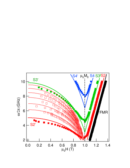
Figure 3: (color online) Dispersions of FMR ($p$ = 0) and SSWs ($p$ = 2 for S2 and S2’, $p$ = 3 for S3 and S3’, $p$ = 4 for S4 and S4’) measured (solid marks) in the entire magnetic field range. Open symbols show the measured lower branches of the DESWs at $H<M_{0}$. Upper branches at $H>M_{0}$, which are too close to the FMR and SSW, are not shown here for brevity but are plotted in Fig. 2 instead. Solid lines are calculated for the SSWs with $p$ = 0, 2, 3 and 4. Dotted lines are calculated for the DESWs with $p$ = 2. The dashed line indicates $H=M_{0}$.

The precisely determined spin boundary conditions allow us to establish a complete picture for the quantized spin excitations. Figure 3 shows the dispersions of the quantized spin waves in the entire field range. At $H>M_{0}$, the solid symbols labelled as FMR, S2, S3 and S4 are FMR ($p$ = 0) and SSWs with $p$ = 2, 3 and 4. Note that the SSWs evolve into the S2’, S3’ and S4’ at $H<M_{0}$. At $H>M_{0}$, the fine structures of the quantized MSFVMs ($p=0$) and DESW ($p=2$), which appear at the lower field side of the FMR and S2, respectively, are not shown in Fig. 3 for clarity. Their dispersions are displayed in Fig. 2 instead. Oscillations between S2’ and S3’ found in Fig. 1(c) at $H<M_{0}$ can now be understood as modes that evolved from the quantized DESW ($p=2$) near S2 at $H>M_{0}$. Resonance positions at the minima of these oscillations are displayed by the open symbols in Fig. 3. We obtain an empirical expression describing the complete spin wave modes with the quantized numbers ($p-\Delta p$, $n$) in the entire field range:

$$\omega^{2} = \gamma^{2}(H_{i}+2Ak^{2}/\mu_{0}M_{0}+P_{p}M_{0})(H_{i}+2Ak^{2}/\mu_{0}M_{0}$$ (3)

$$+M_{0}(1+2n/\pi^{2})(1-P_{p})\sin^{2}\varphi)$$

where $P_{0}=k_{y}d/2$ and $P_{2}=2k_{y}d/\pi^{2}$. Results calculated (curves) using Eq. (3) agree well with experimental data explaination1 . Note that by assuming $n=0$, Eq. (3) reduces to Eq. (2) describing SSWs in the entire $H$ range, and by assuming $\varphi=0$, it agrees with Eq. (2) for the DESW modes at $H>M_{0}$.

In summary, using a highly sensitive photovoltage technique, a comprehensive picture of quantized spin excitations in a single Py microstrip is established. The characteristics of a distinct series of DESW modes allow us to determine precisely the spin boundary condition. The results pave a new way for studying spin dynamics in ferromagnets with finite size, where both the geometrical effect and spin boundary conditions play important roles.

We thank B. Heinrich, G. Williams, H. Kunkel and X. Z. Zhou for discussions, G. Roy for technical support, D. Heitmann, U. Merkt and DFG for the loan of an equipment. N. M. is supported by a DAAD scholarship. This work has been funded by NSERC and URGP.

References

- (1) A. A. Tulapurkar et al., Nature, 438, 339 (2004); J. C. Sankey et al., Phys. Rev. Lett. 96, 227601 (2006).
- (2) G. Prinz and K. Hathaway, Phys. Today, 48(4), 24(1995); S. A. Wolf et al., Science, 294, 1488 (2001).
- (3) J. Jorzick et al., Phys. Rev. B 60 15194 (1999).
- (4) J. Jorzick et al., Phys. Rev. Lett. 88, 047204 (2002).
- (5) Z. K. Wang et al., Phys. Rev. Lett. 89, 027201 (2002).
- (6) J. P. Park et al., Phys. Rev. Lett. 89, 277201 (2002).
- (7) T. G. Rappoport et al., Phys. Rev. B 69, 125213 (2004).
- (8) E. V. Tartakovskaya, Phys. Rev. B 71, R180404 (2005).
- (9) Z. K. Wang et al., Phys. Rev. Lett. 94, 137208 (2005).
- (10) M. Sparks, Phys. Rev. B 1, 3831 (1970); Phys. Rev. Lett. 24, 1178, (1970).
- (11) B. A. Kalinikos and A. N. Slavin, J. Phys. C 19, 7013 (1986).
- (12) R. L. White and I. H. Solt, Phys. Rev. 104, 56 (1956); J. F. Dillon, Jr. , Phys. Rev. 112, 59(1958).
- (13) M. H. Seavey, Jr. and P. E. Tannenwald, Phys. Rev. Lett. 1, 168 (1958).
- (14) G. T. Rado and G. R. Weertman, J. Phys. Chem. Solids 11, 315 (1959); P. Pincus, Phys. Rev. 118, 658 (1960); R. F. Soohoo, Suppl. J. Appl. Phys. 32, 148 (1961); R. F. Soohoo, Phys. Rev. 131, 594 (1963).
- (15) A. H. Morrish, The Physical Principles of Magnetism, (IEEE Press, New York, 2001); C. Kittel, Introduction to Solid State Physics, (John Wiley & Sons, Inc., New York, 1986) 6th ed.
- (16) Y. S. Gui, S. Holland, M. Mecking and C. -M. Hu, Phys. Rev. Lett. 95, 056807 (2005).
- (17) Y. S. Gui, N. Mecking, X. Z. Zhou, G. Williams, and C.-M, Hu, Phys. Rev. Lett. 98, 107602 (2007).
- (18) Spin Dynamics in Confined Magnetic Structures I, edited by Hillebrands and K.Ounadjela (Springer, Berlin, 2002).
- (19) B. Heinrich, in Ultrathin Mangnetic Structures III edited by J. A. C. Bland and B. Heinrich (Springer, Berlin, 2004), Chapter 5, and references therein.
- (20) The discrepancy around is caused by the simplified calculation of , where we assume a perpendicular field direction by neglecting the small tilting angle of 0.2∘. At , this induces an deviation of 36.5 mT for , which causes a resonance frequency discrepancy of about 1.05 GHz.